
Precision prediction of aquaculture water quality: a spatiotemporal model integrating optimized-LSTM and radial basis function neural networks
- Published
- Accepted
- Received
- Academic Editor
- Xiangjie Kong
- Subject Areas
- Algorithms and Analysis of Algorithms, Artificial Intelligence, Computer Vision, Data Mining and Machine Learning, Neural Networks
- Keywords
- Aquaculture water quality, Spatiotemporal prediction, Optimized LSTM, RBF neural network
- Copyright
- © 2026 Shi et al.
- Licence
- This is an open access article distributed under the terms of the Creative Commons Attribution License, which permits unrestricted use, distribution, reproduction and adaptation in any medium and for any purpose provided that it is properly attributed. For attribution, the original author(s), title, publication source (PeerJ Computer Science) and either DOI or URL of the article must be cited.
- Cite this article
- 2026. Precision prediction of aquaculture water quality: a spatiotemporal model integrating optimized-LSTM and radial basis function neural networks. PeerJ Computer Science 12:e3515 https://doi.org/10.7717/peerj-cs.3515
Abstract
Aquaculture water quality parameters are influenced by multiple factors, exhibiting significant temporal and spatial variations. Current prediction methods for these parameters primarily focus on time series predictions at specific observation points, which do not comprehensively characterize the spatiotemporal distribution dynamics of pond water quality parameters. To address this limitation, this study proposes a novel model which incorporates a Self-Attention (SA) mechanism to enhance the capture of long-term dependencies within the data. Furthermore, an enhanced Sparrow Search Algorithm (ESSA) is implemented to optimize the hyperparameters of the long short-term memory (LSTM) network, thereby improving the time series prediction of water quality parameters. Building upon these predictions, the Radial Basis Function (RBF) algorithm is utilized for spatial prediction. The proposed spatiotemporal prediction model, which combines ESSA-SA-LSTM and RBF, demonstrates superior performance by reducing the mean square error (MSE), root mean square error (RMSE), and mean absolute error (MAE) of dissolved oxygen (DO) and water temperature spatiotemporal predictions, outperforming existing comparative algorithms. The model presented in this study significantly enhances the accuracy of spatiotemporal predictions for water quality parameters, playing a crucial role in ensuring the safe production and management of aquatic environments in aquaculture.
Introduction
In aquaculture, maintaining optimal water quality is crucial for the growth, development, and reproduction of aquatic organisms. A well-balanced aquatic environment plays a central role in ensuring the success of aquaculture operations (Li et al., 2020; Jongjaraunsuk, Taparhudee & Suwannasing, 2024; Sabwa et al., 2022; El-Sayed, 2002). Low dissolved oxygen (DO) levels in ponds can lead to reduced metabolic rates, diminished disease resistance, and abnormal swimming behaviors in fish. In severe cases, it can result in surface gulping and even mortality. On the other hand, excessively high DO concentrations can increase the risk of gas bubble disease in fish (Dehghani, Torabi Poudeh & Izadi, 2021; Hafez & Lian-Shin, 2021; Cao et al., 2021; Edouard & Roberto, 2022). Several factors, such as water depth, atmospheric pressure, and temperature, vary spatially and temporally, affecting the prediction of water quality parameters. To reduce the impact of randomness, synergistic effects, and correlations among variables, key water quality parameters are often used as independent variables in predictive models. By integrating these parameters into advanced predictive algorithms, multivariate models can be developed to enhance accuracy (Ustaoğlu, Tepe & Taş, 2020; Zhi et al., 2021; Huan et al., 2020). Traditional water quality monitoring relies on manual sampling, while capable of measuring a wide range of parameters, is labor-intensive, time-consuming, and costly. Additionally, sampled data only represent specific points in time, making large-scale monitoring impractical (Sun et al., 2022; Min et al., 2022; Yi et al., 2022; Dheda & Cheng, 2020). To effectively mitigate aquaculture risks, relying solely on current water quality monitoring data proves insufficient (Zhou et al., 2022). The integration of artificial intelligence with IoT technologies enables intelligent aquaculture systems to not only monitor but also predict future water quality parameter concentrations and their evolving trends. This predictive capability allows for proactive adjustments to maintain optimal water conditions, thereby creating a stable and healthy environment for aquatic organisms. Such technological advancements play a crucial role in preventing water quality deterioration, minimizing farming risks, and promoting the sustainable development of intensive aquaculture practices (Zheng et al., 2023; Eze et al., 2021; Wang et al., 2021; Biazi & Marques, 2023).
Water quality parameters exhibit nonlinear, time-varying, and unstable characteristics due to their susceptibility to various external influencing factors (Feng et al., 2022). Time-series prediction of water quality parameters involves constructing mathematical models and utilizing algorithms to analyze collected data, enabling the forecasting of future trends in water quality over specific time periods (Farsi et al., 2021). Traditional prediction methods, including time-series analysis, grey theory models, and regression analysis, are commonly used (Wu et al., 2022; Panidhapu et al., 2020; Katimon, Shahid & Mohsenipour, 2018). While these models can extract data features and improve prediction accuracy to some extent, they are hindered by time-delay responses and limitations in capturing long-term dependencies within temporal data (Michael, Zhong & Ridha, 2023). In recent years, deep learning models based on neural networks have shown remarkable capability in capturing the nonlinear characteristics of water quality parameters, significantly enhancing prediction performance (Shahi et al., 2020; Dani et al., 2023; Fafoutellis & Vlahogianni, 2023). For instance, Nong et al. (2023) combined Support Vector Regression (SVR) with Random Forest (RF) for DO prediction, achieving a notable improvement in accuracy. However, SVR is sensitive to missing data and computationally demanding during training. In contrast, Artificial Neural Network (ANN) offer greater tolerance for incomplete data. Gautam et al. (2023) applied an ANN model to predict sodium levels in groundwater, demonstrating its reliable accuracy. Adnan et al. (2025) achieved an 85.70% prediction accuracy for biochemical oxygen demand in aquatic environments using an enhanced ANN model. With advancements in deep learning, Recurrent Neural Networks (RNN) have proven more effective than ANN for processing nonlinear time-series data. Zhang, Fitch & Thorburn (2020) integrated Kernel Principal Component Analysis (KPCA) with RNN for DO prediction, achieving an impressive accuracy of 90.80% in one-hour-ahead forecasts. However, RNN are susceptible to gradient vanishing and explosion issues. To overcome these challenges, Hochreiter & Schmidhuber (1997) introduced Long Short-Term Memory (LSTM) networks (Graves, 2012; Heddam et al., 2022). Lee et al. (2022) employed LSTM for real-time DO prediction at the Han River confluence, where ANN models produced accuracy ranging from 0.64 to 0.86, while LSTM models achieved an accuracy of 0.93 to 0.97, further validating LSTM’s superior precision in modeling water quality data. The attention mechanism has gained widespread adoption in water quality prediction due to its ability to enhance the weighting of critical features, demonstrating particular advantages in capturing long-term dependencies among water quality parameters (Cheng et al., 2022; Pranolo et al., 2022; Yan et al., 2022). Huang et al. (2023) achieved exceptional performance (R2 = 99.86%) in predicting water flow velocity by integrating a spatiotemporal attention mechanism with LSTM. Similarly, D et al. (2024) developed an A-LSTM model combining attention mechanisms with LSTM architecture, which attained remarkable prediction accuracy ranging from 98.30% to 99.70% across multiple water quality parameters.
The studies mentioned above highlight the strong performance of LSTM-based deep learning models in the time-series prediction of water quality parameters, demonstrating their capacity to effectively capture complex temporal variations due to their powerful nonlinear modeling capabilities. However, water quality parameters are influenced not only by temporal fluctuations but also by spatial correlations at specific locations. Wang et al. (2025) applied Kriging interpolation for spatial prediction of water quality parameters, achieving mean absolute errors (MAE) of 0.025, 0.025, and 0.074 for DO, pH, and turbidity, respectively. Tayyab et al. (2023) assessed 10 interpolation techniques to predict arsenic concentrations in groundwater resources in Punjab, Pakistan, and found that the Inverse Distance Weighting (IDW) algorithm produced the lowest RMSE and MAE among the tested models. Unlike traditional Kriging and IDW methods, Radial Basis Function (RBF) neural networks do not impose strict requirements on data distribution or geometry, making them well-suited for handling non-uniformly distributed data. This flexibility allows RBF networks to effectively address complex multidimensional prediction challenges. Xie et al. (2024) developed an improved RBF neural network to analyze data from 28 reservoir monitoring stations, and the experimental results demonstrated that the enhanced RBF model outperformed all benchmark models across various evaluation metrics.
The current challenges in aquaculture water quality prediction can be summarized into three key issues: (a) Water quality parameters exhibit high non-linear temporal dynamics and spatial heterogeneity, complicating the ability of a single model to manage them concurrently; (b) Existing deep learning models are sensitive to hyperparameters and are challenging to tune, which limits their application in field deployment scenarios with constrained computational resources; (c) There is a lack of a lightweight and robust predictive interpolation framework tailored for small-scale, highly variable aquaculture pond environments.
To gain a comprehensive understanding of variations in water quality parameters, it is essential to develop a spatiotemporal prediction model that simultaneously considers both temporal and spatial variation patterns. This study proposes a combined model that integrates an enhanced Sparrow Search Algorithm (ESSA), a Self-Attention (SA) mechanism, and an LSTM network to predict water quality parameters in a time-series context across five sampling points. The time-series prediction results are subsequently utilized as inputs for a RBF network to facilitate spatial predictions. By merging time-series and spatial prediction techniques, this study constructs a spatiotemporal prediction model that effectively captures long-term dependencies in temporal data while incorporating spatial correlations. The resulting model provides accurate spatiotemporal forecasting of water quality parameters, offering valuable technical support for water quality monitoring and management.
Materials and Methods
Study area and data acquisition
The study focuses on an irregularly shaped aquaculture water area located at coordinates 32∘18′50″N, 120∘35′31″E, in Changzhou City, China, as depicted in Figs. 1A and 1B. This area measures approximately 150 m in length, 45 m in width, and 2 m in depth. The spatial environment of this region is well-preserved, with no surrounding pollution sources. During the deployment of the buoys, they were strategically positioned at various locations. Each buoy was equipped with multiple sensors installed at the same depth, ensuring uniformity across the sensors on each individual buoy. However, the deployment depths of the sensors varied among different buoys, ranging from 0.3 m to 1.9 m. To provide a clearer illustration of this arrangement, we have included a schematic diagram, as shown in Figs. 1C and 1D. The sensors, housed within waterproof enclosures, are detailed in Table 1. The collected water quality data includes DO concentration, water temperature, pH, ammonia nitrogen level, and ORP, with measurements recorded at 10-min intervals.
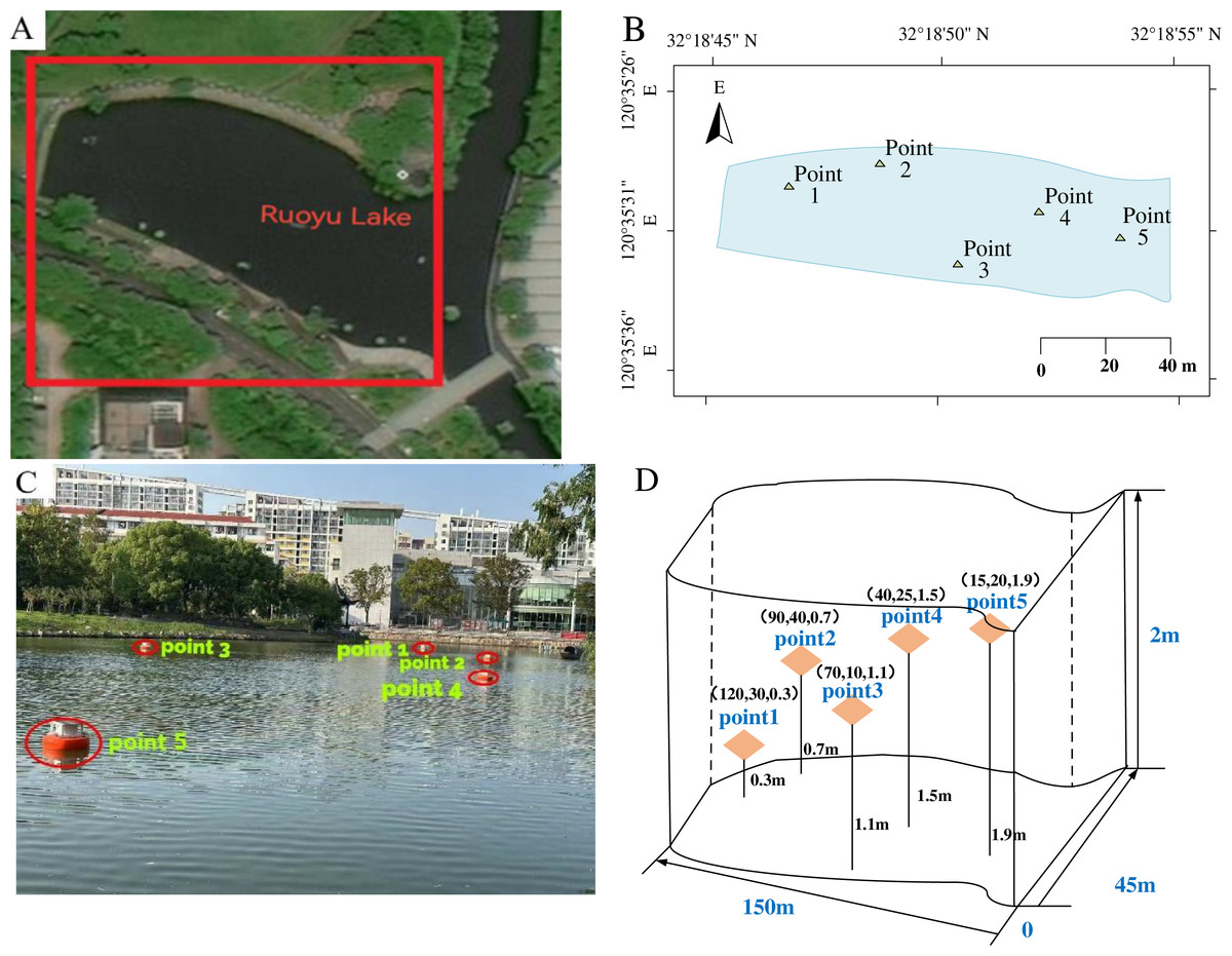
Figure 1: Study area and deployment of measuring points.
(A) Aerial view of the study area. (B) Geographic location of the study area. (C) Schematic layout of the monitoring points. (D) Coordinates of sensors placement.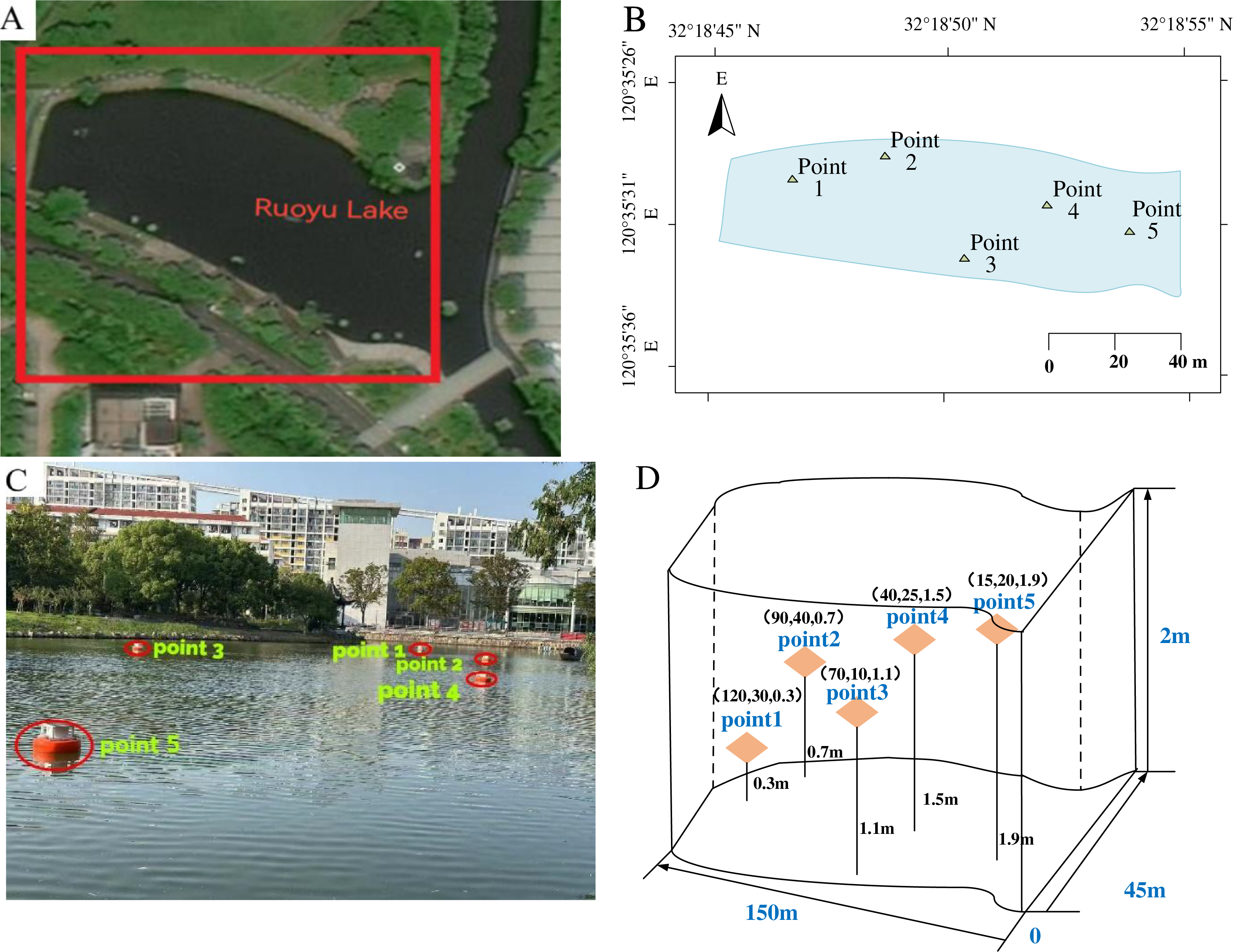
| Sensor type | Model | Measurement range | Measurement error |
|---|---|---|---|
| DO sensor | JXSZ-1001-DOY | 0–20 (mg/L) | 0.01 (mg/L) |
| Water temperature sensor | DS18B20 | −10 – +85 (°C) | 0.5 (°C) |
| pH sensor | PHG-206A | 0–14 (pH) | 0.1 |
| Ammonia nitrogen sensor | NHN-206A | 0–100 (mg/L) | 0.01 (mg/L) |
| ORP sensor | ORP-206A | −1,500 – +1,500 (mV) | 10 (mV) |
Data preparation
For the missing data in sensor collection, the adjacent data collected under the same conditions are utilized to estimate the missing values, as demonstrated in Eq. (1).
(1) where represents the missing sensor data at time , while and denote the original sensor data at times and , respectively.
Given that water quality data and meteorological data exhibit continuity and temporal sequence, any instance where the variation range of continuously collected data exceeds that of the preceding and succeeding moments is identified as an outlier. These outliers are subsequently processed horizontally utilizing the mean smoothing method, as illustrated in Eq. (2).
(2) where denotes the outlier at time , while and represent the valid neighboring values at the adjacent time points.
Upon partitioning the collected data into training and testing sets, normalization is subsequently applied, as demonstrated in Eq. (3).
(3) where represents the normalized value, X denotes the original data, and and correspond to the maximum and minimum values of the original sequence, respectively.
The research collected data samples over a 32-day period, specifically from March 15 to April 15, 2024. The dataset was divided into training and testing sets with a ratio of 70:30. Table 2 presents a representative subset of the raw data collected during the monitoring period of 2024.
| Data | Time | pH | DO (mg/L) | Ammonia nitrogen (mg/L) | Water temperature (°C) | ORP (mV) |
|---|---|---|---|---|---|---|
| 3–15 | 01:00 | 8.32 | 9.37 | 1.33 | 16.31 | 361 |
| 3–15 | 02:20 | 8.41 | 9.47 | 1.33 | 16.42 | 363 |
| 3–15 | 08:30 | 8.21 | 9.44 | 1.34 | 17.33 | 370 |
| 3–15 | 12:20 | 8.25 | 9.50 | 1.35 | 20.53 | 390 |
| 3–15 | 16:10 | 9.29 | 9.32 | 1.38 | 22.16 | 370 |
| 3–15 | 20:50 | 8.21 | 9.18 | 1.35 | 19.87 | 3,634 |
| 3–16 | 00:00 | 8.13 | 9.22 | 1.34 | 16.54 | 392 |
| 3–16 | 03:10 | 7.63 | 8.78 | 1.35 | 16.75 | 389 |
| 3–16 | 08:30 | 7.62 | 8.84 | 1.36 | 17.21 | 383 |
| 3–16 | 12:50 | 7.68 | 8.91 | 1.44 | 21.32 | 303 |
| 3–16 | 13:10 | 7.68 | 9.28 | 1.43 | 21.47 | 289 |
| 4–15 | 16:00 | 7.67 | 9.04 | 1.52 | 21.33 | 413 |
| 4–15 | 17:40 | 7.64 | 8.67 | 1.45 | 21.21 | 416 |
Model’s performance evaluation metrics
To comprehensively evaluate the predictive performance of the model, this study utilizes three key evaluation metrics: RMSE, MAE, and the Coefficient of Determination (R-squared, R2). Superior model is indicated by lower values of RMSE and MAE, along with a higher R2 value. The mathematical formulas for these metrics are presented in Eqs. (4) to (6).
(4)
(5)
(6) where represents the observed value of the water quality parameter, represents the predicted value of the water quality parameter, is the sample size, and is the mean value of the water quality parameter.
Descriptions of the proposed models
To improve the spatiotemporal prediction accuracy of aquaculture water quality parameters, this study proposes an innovative prediction model that integrates ESSA-SA-LSM with RBF neural networks.
(1) SA-LSTM model
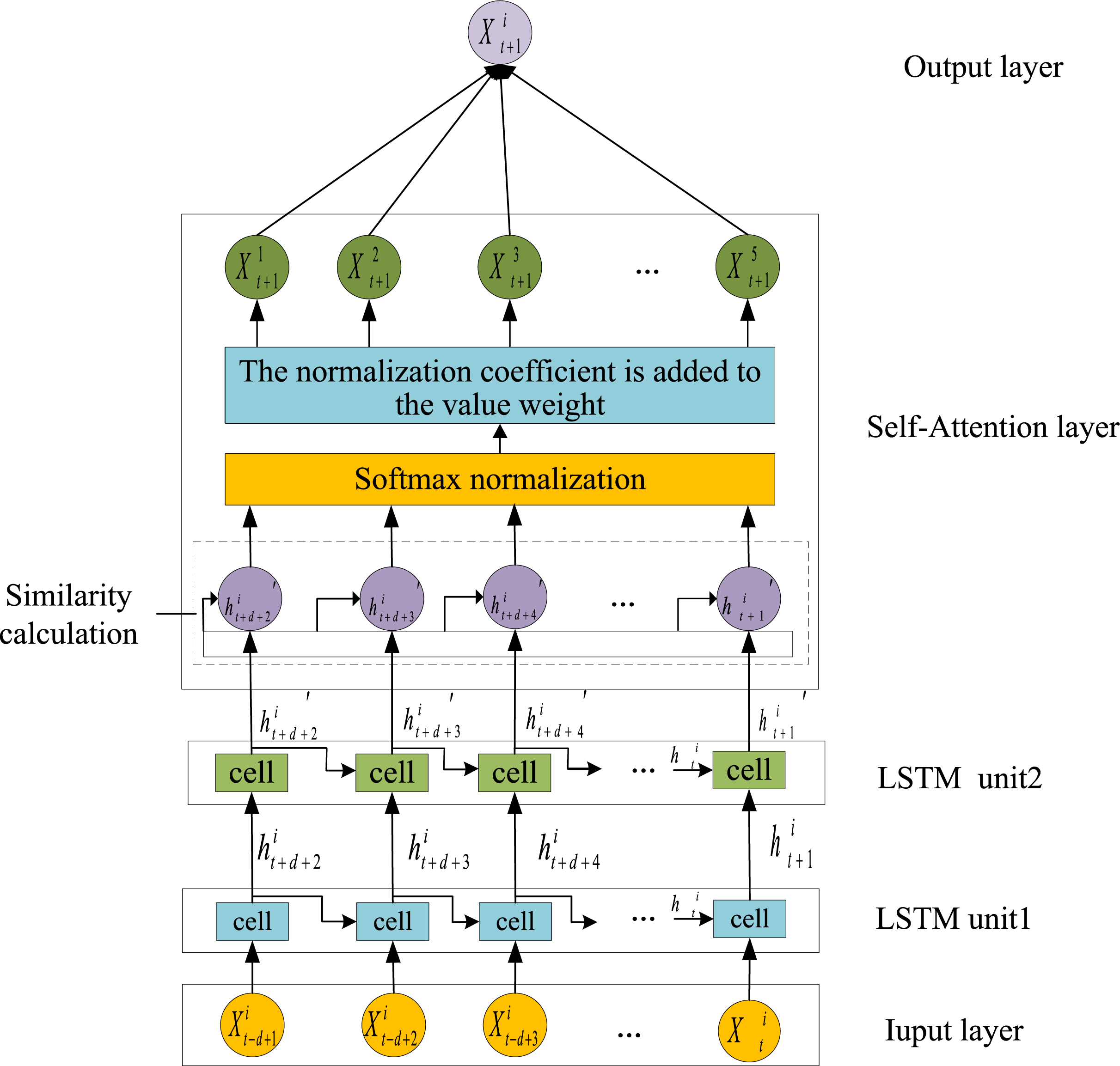
The primary objective of this study is to address the challenge of time series prediction for forecasting future water quality parameters based on historical data. To achieve this, an LSTM model is employed to construct a foundational prediction framework, which effectively captures the sequential temporal dependencies inherent in water quality parameters. Furthermore, the model is enhanced by incorporating a self-attention mechanism, leading to the proposed SA-LSTM prediction model. The architecture of the proposed model is depicted in Fig. 2.
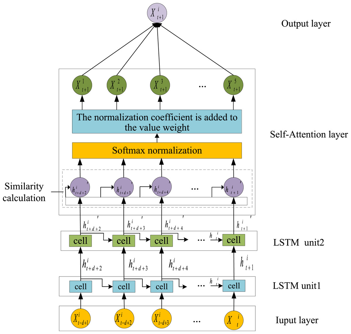
Figure 2: Time series prediction structure diagram.
The time step of the LSTM is represented by d, with a value of 6. The processed data from time t−d+1 to t, including pH, ammonia nitrogen, water temperature, DO, and ORP ( to ), are utilized as inputs to the SA-LSTM model. Initially, feature extraction is conducted using the LSTM network. Subsequently, the data are fed into the self-attention mechanism to capture the relationships between the current time step and historical water quality parameter data, assigning higher weights to more significant time steps. An improved SSA is employed to optimize the hyperparameters of the LSTM network. Finally, the model predicts water quality parameters, outputting the spatiotemporal predictions of pH, ammonia nitrogen, water temperature, DO, and ORP at time t+1 as to .
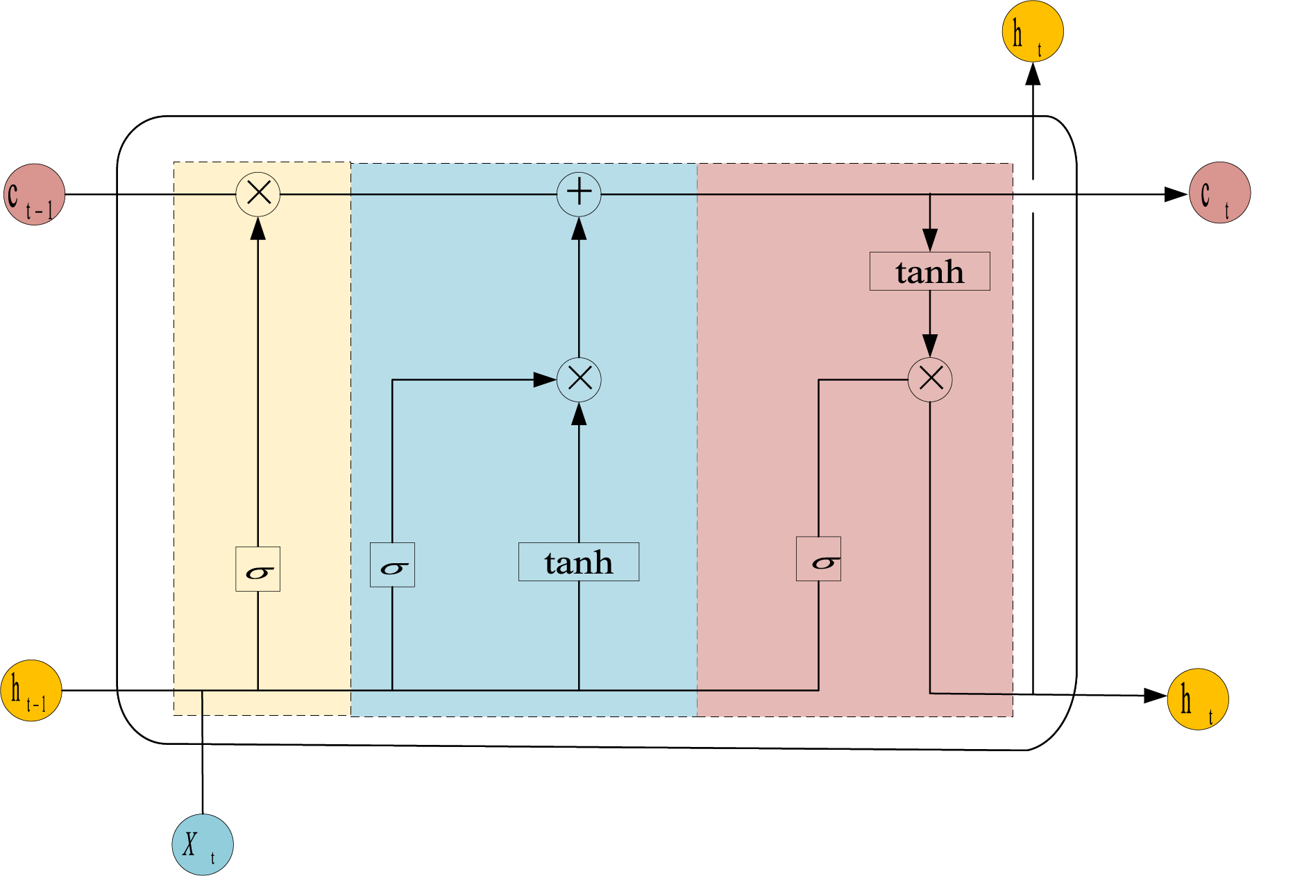
The LSTM model is a specialized architecture of RNN that incorporates gating mechanisms and hidden states to handle the problems of gradient explosion and vanishing gradients when managing long-term dependencies. In contrast to traditional RNNs, LSTM introduces gating units that regulate the flow of information, allowing the model to retain significant data and essential features while discarding irrelevant information. The cell architecture of the LSTM is depicted in Fig. 3, and the computational processes for the forget gate ( ), input gate ( ), output gate ( ), cell state ( ) and output ( ) are presented in Eqs. (7) to (12).
(7)
(8)
(9)
(10)
(11)
(12) where denotes the value labeled by time; tanh represents the hyperbolic tangent function, which outputs values in the range (−1, 1); , and are constant biases; and , and correspond to the weight matrices associated with the input gate, output gate, and the conveyor belt mechanism, respectively.
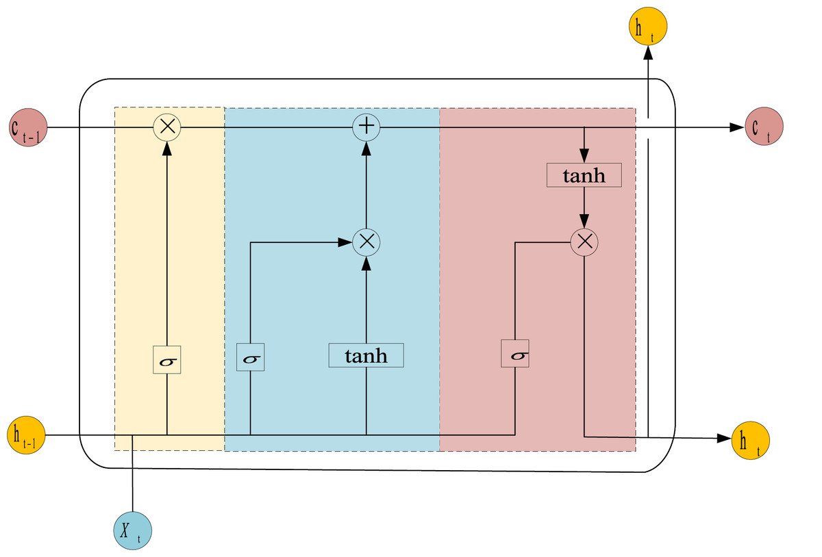
Figure 3: Structure of LSTM unit.
SA represents a significant advancement in attention mechanisms, offering two primary benefits: it facilitates the efficient extraction of critical information while minimizing attention to irrelevant data, and it concurrently reduces reliance on external information sources, thereby enhancing the capacity to capture intrinsic relationships within input data. By integrating the self-attention mechanism, the LSTM can effectively address challenges related to information overload, while simultaneously improving predictive accuracy and system robustness.
The attention mechanism is fundamentally based on three parameters: Q, K, and V. The output of LSTM, denoted as , serves as the input for the SA module. The output of the SA module, denoted as , is calculated as illustrated in Eq. (13).
(13)
The predicted value of the target water quality parameter is presented in Eq. (14).
(14) where represents the output weight matrix of the fully connected network, and denotes the output bias vector across the entire network structure.
(2) ESSA module
The SSA, a swarm intelligence-based optimization technique, is widely recognized for its robust optimization capabilities and rapid convergence. However, the standard SSA implementation exhibits certain limitations that hinder its performance. Firstly, the random initialization of sparrow population positions at the algorithm’s inception results in limited population diversity, consequently yielding suboptimal target solutions that adversely affect the algorithm’s iterative performance and error rates. Secondly, the discoverers in SSA tend to exhibit excessive aggressiveness during food source exploration. Upon locating an optimal solution, other individuals rapidly converge towards it, thereby diminishing population diversity and increasing susceptibility to local optima. Furthermore, the underutilization of the finder’s positional information may cause the algorithm to overlook potential optimal regions, thereby missing valuable exploration opportunities. To address these limitations, this study proposes the ESSA module that incorporates two key improvements: (1) composite chaos mapping for population initialization and (2) an adaptive inertial weight factor. These modifications aim to optimize the hyperparameters of LSTM neural networks, effectively resolving issues related to slow parameter convergence and inadequate global search capabilities. Specifically, the improved Tent-Logistic-Cosine composite mapping enhances the initial positioning of sparrows, as detailed in Eqs. (15)–(17), while the adaptive inertia weight factor and finder position optimization are mathematically formulated in Eqs. (18)–(19).
(15) where represents the sequence value at the i-th iteration, and denotes the control parameter that governs the system’s behavior.
When and , Eq. (13) is normalized to constrain its range within the interval [0, 1], as expressed by Eq. (16).
(16) where represents the absolute value function, while serves as the normalization constant.
The final initialization of sparrow positions is given by Eq. (17).
(17) where represents the initial coordinate of the sparrow in the dimension, where and denote the lower and upper bounds of the dimension, respectively. The dimension j corresponds to the parameter to be optimized, with in the current implementation. Specifically, the parameter ranges are defined as follows: the learning rate is bounded within [0.001, 0.1], the iteration number is constrained to [10, 1,000], and the number of hidden layer neurons is limited to [1, 100].
(18)
(19) where represents the adaptive inertia weight factor, where is set to 0.9 and to 0.3. The variable denotes the current iteration index, and j indicates the dimensionality of the parameters to be optimized represents the position of the sparrow in the dimension at the iteration. The term L denotes a unit row vector, and is a random number uniformly distributed in the interval [0, 1]. The maximum iteration count is denoted by and Q represents a random number following the standard normal distribution. The warning threshold satisfies , and the safety threshold is bounded within the range [0.5, 1].
The ESSA module is employed to optimize four critical hyperparameters of the SA-LSTM model: the learning rate, iteration count, neuron count in the first hidden layer, and neuron count in the second hidden layer. The optimization procedure consists of the following specific steps:
-
(a)
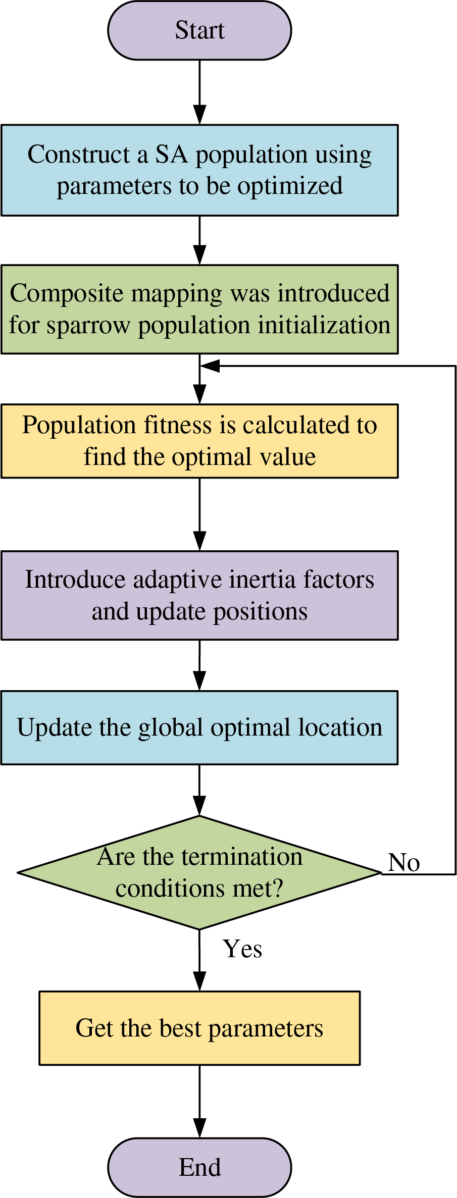
Initialization: Configure the population size and the proportion of discoverers, joiners, and alarmers within the SSA module. The population is initialized using the Tent-Logistic-Cosine composite mapping to ensure a more uniform distribution of the initial population.
-
(b)
Parameter Space Definition: Define the dimensionality of the parameter space and establish the search boundaries for each parameter, thereby determining the initial positions of the sparrow population.
-
(c)
Fitness Evaluation: Calculate the fitness value for each sparrow using the error function, identifying the optimal fitness value and its corresponding position.
-
(d)
Position Update: Incorporate the adaptive inertia factor to update the positions of discoverers, joiners, and alarmers through the improved dynamic step size mechanism.
-
(e)
Termination Check: Re-evaluate the fitness values of the sparrow population. If the error falls within the target threshold, terminate the iteration; otherwise, return to step (d) for further optimization.
The workflow of the ESSA module is depicted in Fig. 4.
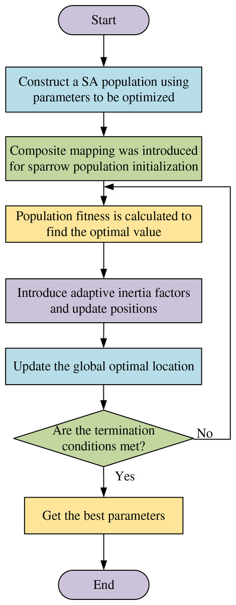
Figure 4: Workflow of the ESSA.
(3) Spatial prediction models
The key water quality parameters exhibit distinct three-dimensional distribution characteristics in large surface ponds. Significant variations are observed both across different water layers within the same vertical plane and at different positions within the same water layer. Consequently, measurements from a single point cannot adequately represent the overall water quality dynamics of the entire pond. To better characterize the spatiotemporal distribution of these critical parameters, a three-dimensional spatial analysis method is employed, enabling comprehensive monitoring of water quality parameter distributions throughout the pond.
To enhance the interpolation accuracy of water quality parameters, this study utilizes the RBF for interpolating prediction results. The coordinates of the RBF centers are determined from the training data using the k-means clustering algorithm. For each RBF center, the width parameter is calculated based on the average distance from this center to its nearest neighboring centers, expressed by Eq. (20). To mitigate the risk of overfitting, regularization is applied when solving for the output layer weights.
(20) where = 3 is a predefined hyperparameter that represents the number of the nearest neighboring centers considered; is the RBF center; is the nearest neighbor of center ; represents the Euclidean distance between the two centers.
The spatiotemporal prediction outcomes are demonstrated using DO as a representative example. Figure 5 illustrates the structural framework of the RBF-based spatiotemporal prediction model. The model incorporates data from the three sensors nearest to the interpolation point at time as input, generating predictions for both water temperature and DO values at the specified interpolation point and time.
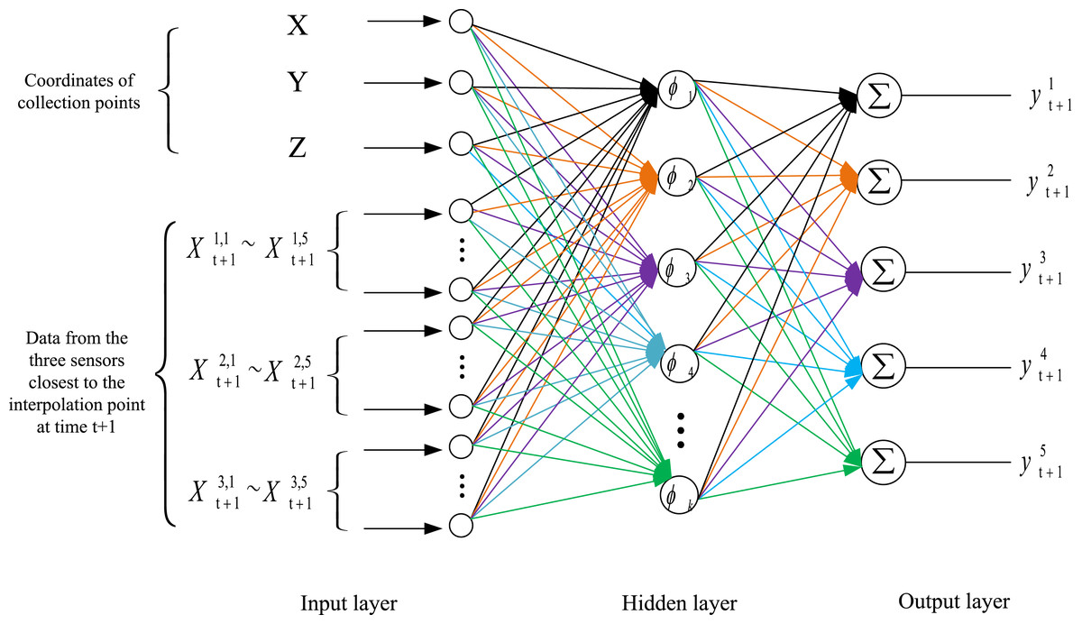
Figure 5: Structural framework of the RBF.
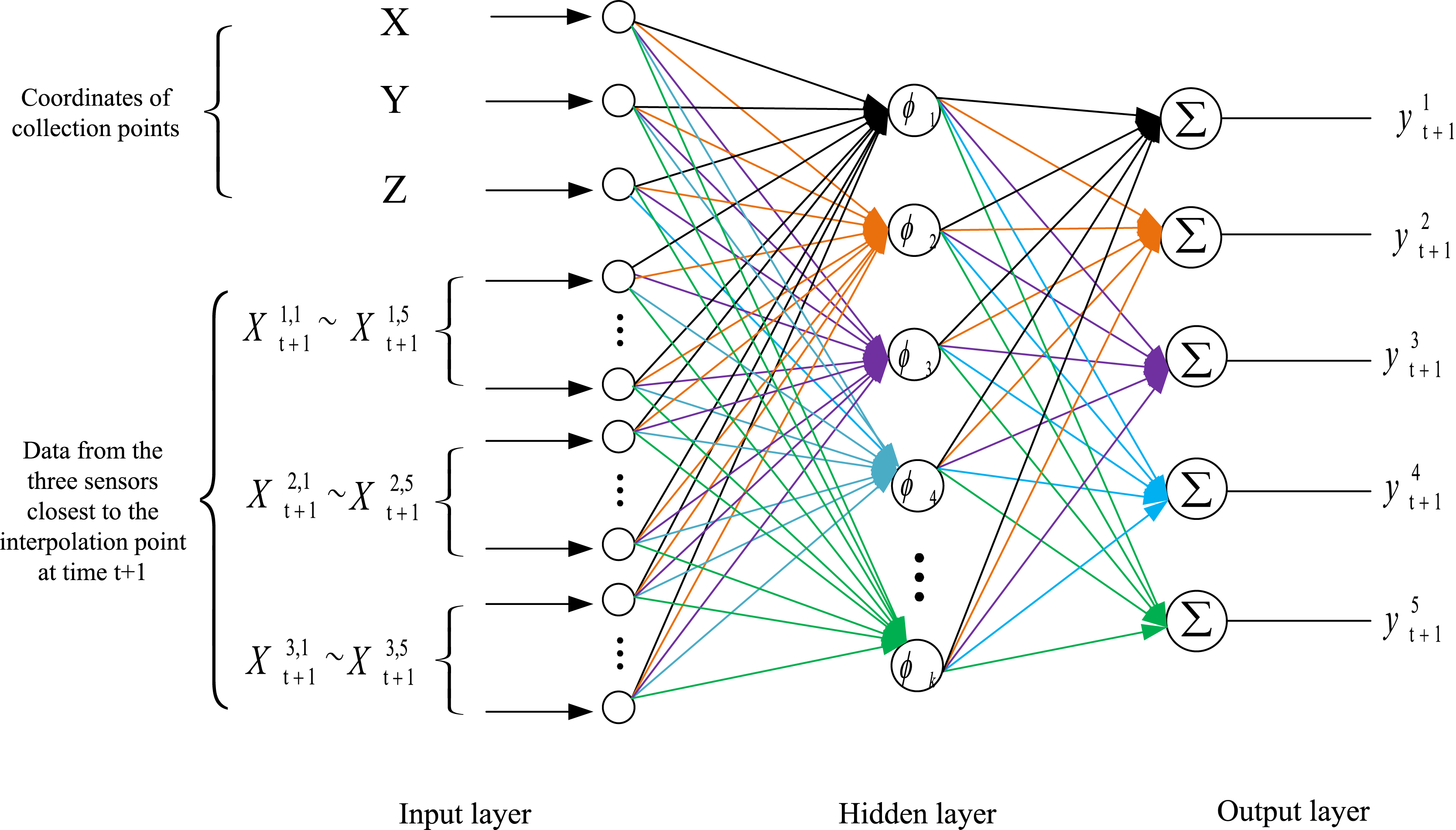
This process begins with the construction of a RBF network and the initialization of its parameters. Subsequently, the time series prediction results at time from the three monitoring points nearest to the target prediction location are used as inputs to the RBF network. Specifically, 15 data points, represented as , and , are employed to predict the target point’s pH, ammonia nitrogen, water temperature, DO, and ORP values ( ) at time .
Results and discussions
The experimental setup in this study comprised a computing system with the following specifications: an Intel Core i5-8265U processor, 16 GB of RAM, and the Windows 10 operating system. The computational framework was implemented using Python 3.10 through the Anaconda distribution platform. For model training, the experimental protocol employed the gradient descent optimization algorithm with the following parameters: a batch size of 32 samples, an input sequence length (time steps) of 6, and 1,000 training epochs. The Adam optimizer was employed with an initial learning rate of 0.001. To mitigate overfitting, the dropout rate was set to 0.3. The key parameters of the ESSA adopted in this study are shown in Table 3.
| Parameter | Value |
|---|---|
| Population size | 50 |
| Discoverers ratio | 20% |
| Joiners ratio | 70% |
| Alerters ratio | 10% |
| R2, Alert value | 0.8 |
| ST, Safety threshold | 0.6 |
| Max iterations | 1,000 |
This study identifies the optimal combination of three key hyperparameters of the SA-LSTM model using the ESSA algorithm. The specified search ranges for optimization and the final results of the ESSA-SA-LSTM model are presented in Table 4.
| Optimized parameter | Search range | Optimal value |
|---|---|---|
| Initial learning rate | [0.001, 0.01] | 0.00369 |
| Epochs | [10, 1,000] | 512 |
| Hidden neurons | [1, 1,000] | 81 |
Ablation experiments
To comprehensively evaluate the predictive performance of the proposed ESSA-SA-LSTM model, systematic ablation experiments were conducted using LSTM as the baseline model. The experimental design included three key components: the baseline LSTM, SA mechanism and ESSA optimization. The comparative results of these experiments are presented in Table 5.
| Group | LSTM | SA | ESSA | RMSE | MAE | |
|---|---|---|---|---|---|---|
| 1 | ✓ | 0.0384 | 0.0287 | 0.9285 | ||
| 2 | ✓ | ✓ | 0.0305 | 0.0270 | 0.9551 | |
| 3 | ✓ | ✓ | ✓ | 0.0157 | 0.0122 | 0.9881 |
The proposed model demonstrates significant performance improvements across all evaluation metrics compared to alternative architectures. Specifically, when compared to the SA-LSTM model, it achieves an average reduction of 48.52% in RMSE and 54.81% in MAE, while improving the value by an average of 3.46%. More substantial enhancements are observed relative to the LSTM model, with average reductions of 59.11% in RMSE and 57.49% in MAE, respectively, along with an average increase of 6.42% in .
These performance gains can be attributed to three key innovations: (1) the implementation of correlation analysis on the original data, which effectively reduces computational redundancy; (2) the integration of a self-attention mechanism that mitigates information loss during sequential processing; (3) the incorporation of composite mapping and adaptive inertia factors within the enhanced SSA algorithm, which optimizes LSTM parameters, accelerates convergence, and enhances global search capabilities, ultimately improving overall model performance. The proposed model requires less than 10 MB of memory and achieves an average inference time of under 20 ms during training, both of which are entirely acceptable. In scenarios that demand even faster execution, the inference time can be significantly reduced by strategically compromising the density of the spatial prediction points.
Comparison of experimental results on time-series sequence
The model proposed in this study is benchmarked against the SA-LSTM, and standard LSTM models, all of which utilize identical datasets. Using Point 1 (Fig. 1D) as a case study, the comparative performance across five key variables is illustrated in Figs. 6A to 6E. The performance metrics reveal substantial improvements: compared to the SA-LSTM model, the proposed model achieves reductions of 75.00% in RMSE and 73.24% in MAE, along with a 3.37% increase in R2. More significant enhancements are observed relative to the LSTM model, with 80.91% and 79.12% reductions in RMSE and MAE, respectively, and a 6.40% improvement in . These results substantiate that the proposed model not only accurately tracks the temporal dynamics of dissolved oxygen and water temperature variations but also effectively predicts their absolute values. The comprehensive evaluation confirms the superior predictive capabilities of the proposed architecture over existing models.
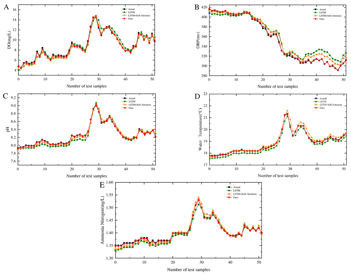
Figure 6: Performance of different models across five water quality parameters.
(A) Prediction performance of DO for different algorithms. (B) Prediction performance of ORP for different algorithms. (C) Prediction performance of pH for different algorithms. (D) Prediction performance of water temperature for different algorithms. (E) Prediction performance of ammonia nitrogen for different algorithms.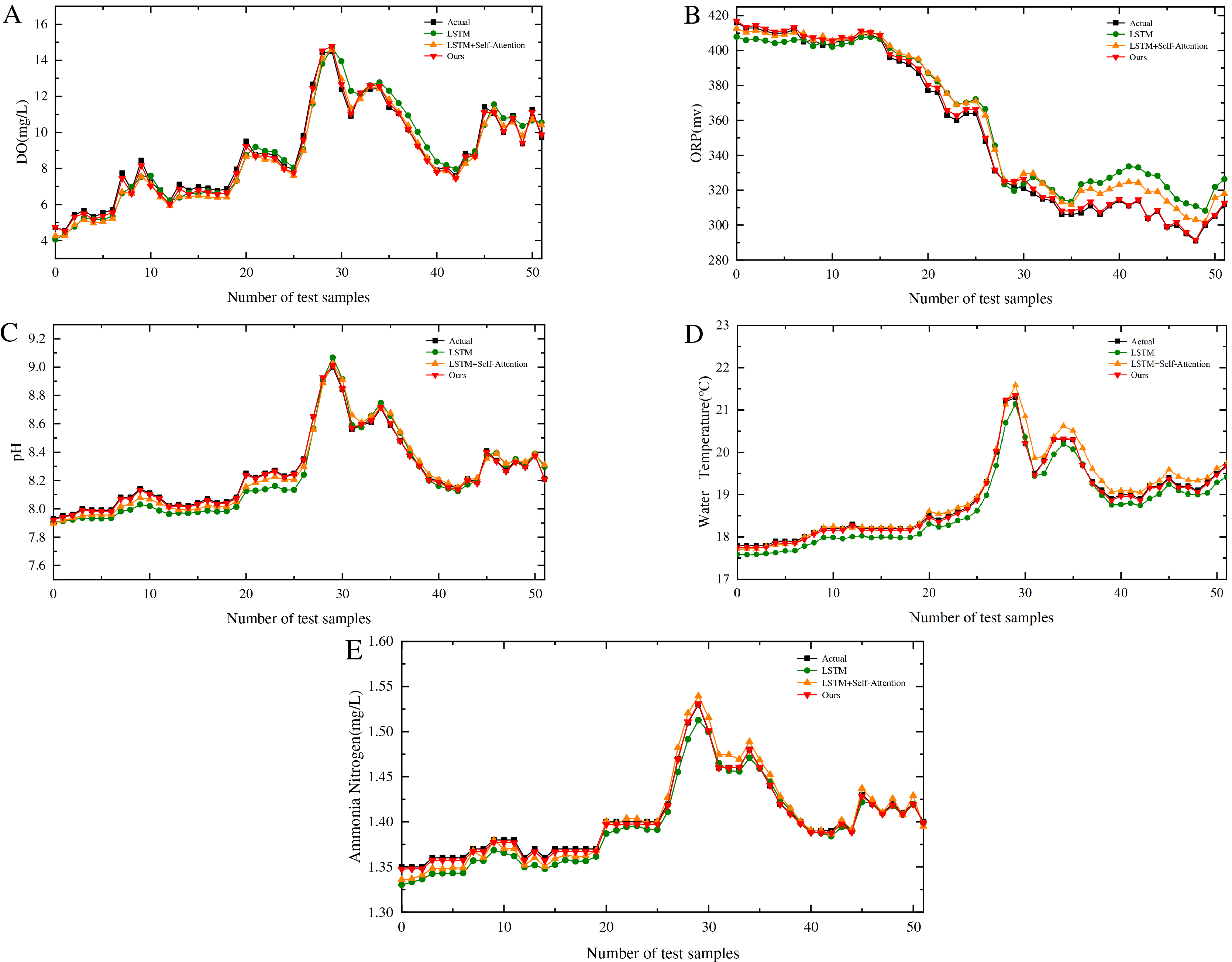
The proposed model demonstrates a significant enhancement in performance across all five water quality parameters compared to the other two models. Significance testing reveals that all -values are substantially below the 0.05 threshold, indicating highly statistically significant differences. These results further substantiate the superiority of the model presented in this study.
Spatiotemporal distribution prediction of water quality parameters
Using DO and water temperature as representative cases, the collected dataset reveals distinct diurnal patterns with observable peaks occurring at 12:00 and 24:00. This temporal variation underscores the necessity of developing accurate spatiotemporal distribution models for these critical water quality parameters at these specific time points. To address this, the study employs the ESSA-SA-LSTM model to predict DO and water temperature levels at 12:00 and 24:00 on April 15, 2024. These prediction results subsequently serve as input data for comprehensive spatiotemporal analysis. The spatial prediction component was implemented using the Python computational platform. For enhanced visualization and analysis of the spatiotemporal distribution patterns, the model incorporates RBF interpolation to generate detailed distribution maps. Figure 7 presents the spatial distribution characteristics of DO and water temperature at both 12:00 and 24:00, with subfigures 7A through 7D providing comprehensive visual representations of these patterns.
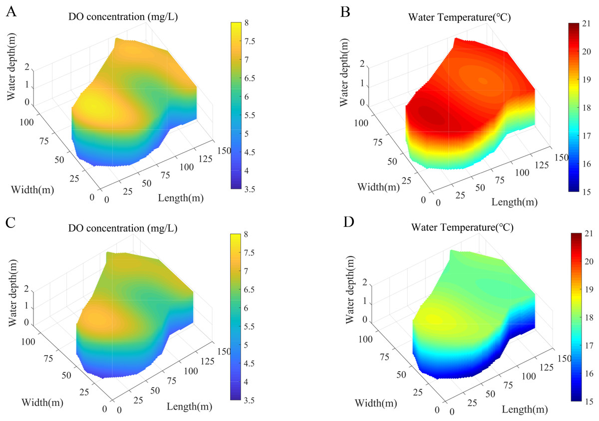
Figure 7: Spatiotemporal distribution prediction of DO and water temperature at 12:00 and 24:00.
(A) Predicted DO distribution at 12:00. (B) Predicted water temperature distribution at 12:00. (C) Predicted DO distribution at 24:00. (D) Predicted water temperature distribution at 24:00.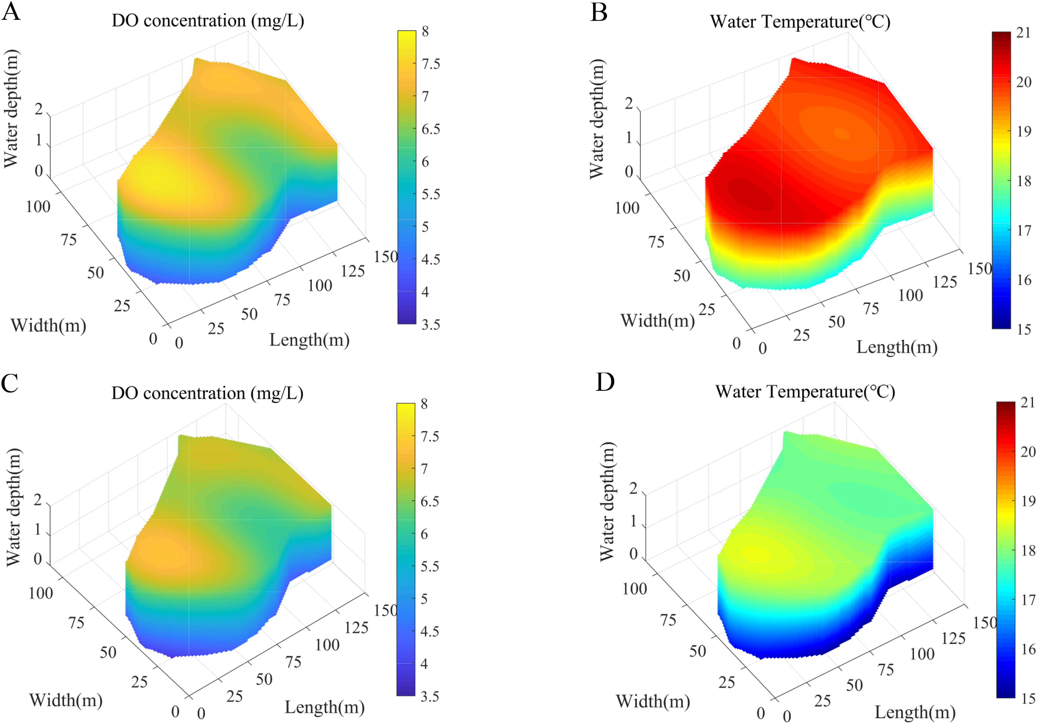
As illustrated in Figs. 7A and 7C, the spatiotemporal distribution of dissolved oxygen exhibits distinct vertical stratification, with DO concentration progressively decreasing with increasing depth from the water surface. This phenomenon can be attributed to the primary mechanism of oxygen production in aquatic systems-photosynthesis by phytoplankton and aquatic plants, which predominantly inhabit the surface and littoral zones. As depth increases, photosynthetic activity diminishes due to light attenuation caused by water refraction and turbidity, consequently reducing oxygen production and resulting in lower dissolved oxygen levels in deeper water layers. Similarly, Figs. 7B and 7D reveal a comparable vertical temperature gradient, with water temperature decreasing as distance from the surface increases. This thermal stratification pattern results from the extensive exposure of the surface layer to solar radiation, creating a temperature differential between the warmer surface waters and cooler deeper layers.
To comprehensively evaluate the performance of the proposed RBF method, we conducted comparative experiments using ESSA-SA-LSTM integrated with two alternative interpolation approaches: IDW and linear triangular interpolation. The evaluation was performed on identical datasets to ensure fair comparison. The study employed a cross-validation methodology to assess the accuracy of each algorithm. Table 6. presents the spatiotemporal prediction accuracy metrics for DO and water temperature across all evaluated algorithms. The results demonstrate that, compared to ESSA-SA-LSTM with linear triangular interpolation and ESSA-SA-LSTM with IDW, the proposed ESSA-SA-LSTM-RBF approach achieved reductions in MSE of 38.49% and 48.08%, respectively. Similarly, RMSE decreased by 35.15% and 27.96%, while MAE showed reductions of 15.09% and 3.68%, respectively. Through a comparative analysis of interpolation accuracy for DO and water temperature, the results indicate that the proposed algorithm exhibits superior performance, particularly in scenarios with limited monitoring points. This enhanced performance is attributed to the RBF method’s ability to effectively handle sparse data distributions while maintaining interpolation accuracy.
| Algorithm | MSE | RMSE | MAE |
|---|---|---|---|
| Ours | 0.1892 | 0.4349 | 0.3853 |
| ESSA-SA-LSTM-Linear triangular interpolation | 0.3076 | 0.6706 | 0.4538 |
| ESSA-SA-LSTM-IDW | 0.3644 | 0.6037 | 0.4000 |
Conclusion
To precisely characterize the spatiotemporal distribution of DO and water temperature in aquaculture ponds and mitigate associated farming risks, this study proposes an innovative algorithm that integrates an enhanced sparrow search algorithm with a SA-LSTM and RBF. The primary contributions and findings can be summarized as follows:
-
(1)
For the time-series prediction of water quality parameters, the proposed methodology first employs a self-attention mechanism to capture intrinsic correlations within the data and highlight the influence of key features in the input data. Subsequently, an improved sparrow search algorithm is implemented to optimize the hyperparameters of the LSTM network. Finally, ablation experiments demonstrate that the proposed time-series prediction model significantly enhances the accuracy of water quality parameter forecasting.
-
(2)
Comprehensive comparative experiments demonstrate the superior performance of ESSA-SA-LSTM-RBF, showing significant improvements over alternative approaches. Specifically, compared to ESSA-SA-LSTM with linear triangular interpolation and ESSA-SA-LSTM-IDW algorithms, the proposed method achieves reductions in MSE of 38.49% and 48.08%, respectively. Similarly, RMSE values decrease by 35.15% and 27.96%, while MAE improvements reach 15.09% and 3.68%, respectively. These results confirm the enhanced predictive capabilities of the proposed algorithm over conventional methods.
-
(3)
In the next phase of our research, we will systematically incorporate models such as GRU, Bi-LSTM, TCN, and the classical ARIMA model into our comparative framework. A rigorous hyperparameter tuning process will be conducted for these models to ensure a comprehensive performance evaluation. Furthermore, we will introduce additional spatial interpolation algorithms, such as Kriging, for comparative analysis. Confidence intervals and statistical tests will also be implemented to ascertain whether the observed differences are statistically significant. We also plan to systematically collect monitoring data from ponds and similar water bodies across various seasons, such as summer and autumn, as well as from different geographical locations. Incorporating multi-source external driving factors is essential for enhancing the model’s physical interpretability and generalization performance. Meanwhile, the analysis of the model’s time complexity will be performed to rigorously establish its practical feasibility and scalability.
The developed spatiotemporal model offers dual advantages: it not only enhances the accuracy of time series predictions but also improves the precision of spatial predictions. This advancement provides a robust theoretical foundation for intelligent aquaculture systems.
Supplemental Information
Comparison prediction data of four models.
The data point indicates output of the four models.