
The analysis of voltage collapse induced by nonlinear loads in an arc furnace utilising deep learning-driven TabNet and NODE models
- Published
- Accepted
- Received
- Academic Editor
- Ankit Vishnoi
- Subject Areas
- Algorithms and Analysis of Algorithms, Artificial Intelligence, Data Mining and Machine Learning, Data Science, Neural Networks
- Keywords
- Electric arc furnaces (EAF), Explainable AI (XAI), LIME, NODE, SHAP, TabNet, Voltage collapse prediction
- Copyright
- © 2026 Asal et al.
- Licence
- This is an open access article distributed under the terms of the Creative Commons Attribution License, which permits unrestricted use, distribution, reproduction and adaptation in any medium and for any purpose provided that it is properly attributed. For attribution, the original author(s), title, publication source (PeerJ Computer Science) and either DOI or URL of the article must be cited.
- Cite this article
- 2026. The analysis of voltage collapse induced by nonlinear loads in an arc furnace utilising deep learning-driven TabNet and NODE models. PeerJ Computer Science 12:e3505 https://doi.org/10.7717/peerj-cs.3505
Abstract
Electric arc furnaces (EAF) represent a class of nonlinear loads distinguished by high energy consumption during metal melting processes. Voltage collapses in these systems adversely affect power quality, reduce energy efficiency, and cause significant disruptions in production processes. Consequently, this study investigates the feasibility of deep learning-based approaches for forecasting voltage collapse events induced by the dynamic and nonlinear loads generated by electric arc furnaces. The analysis employs methods developed using the Tabular Network (TabNet) and Neural Oblivious Decision Ensembles (NODE) models to assess the characteristic variations of arc furnaces and their impacts on power systems through both experimental and simulation data. The characteristic behavior of the electric arc was modeled using an exponential-hyperbolic function validated by real-time data, while the simulation model was established in the MATLAB/Simulink environment to identify voltage collapse events. Critical features such as I1 (current) and V1 (voltage) were found to play a decisive role in predicting voltage collapse, and the decision mechanisms of the models were elucidated in detail using Explainable Artificial Intelligence (XAI) techniques such as SHapley Additive exPlanations (SHAP) and Local Interpretable Model-agnostic Explanations (LIME). The obtained results indicate that both models achieve an accuracy rate of approximately 95% with balanced classification performance, thereby offering a reliable approach for the early diagnosis of voltage fluctuations and collapse events in power systems. Furthermore, the findings contribute to strategic decision support systems aimed at enhancing safety and energy efficiency in industrial applications and offer a novel perspective on the potential of deep learning models in complex systems.
Introduction
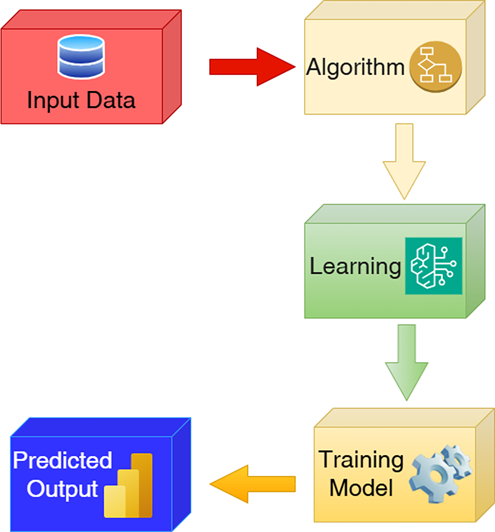
Historically, there has been considerable debate on whether voltage collapses are static or dynamic and they can be analyzed as a load flow problem, in addition to whether they can be analyzed with differential equations. Researchers have studied the load flow feasibility of voltage collapses (Galiana, 1984), optimal power flow analysis (Carpentier, 1984) and steady state issues (Brucoli et al., 1985). Kwatny, Pasrija & Bahar (1986) studied the voltage collapse problem as a bifurcation defined by the disappearance of an equilibrium point. They proposed how this bifurcation can explain the instability of the voltage. The basic components of a power system are presented in Fig. 1. Schleuter et al. (1987) and Costi, Shu & Schlueter (1986) introduced the concepts of voltage stability and controllability in power systems. The control criteria they introduced in their work form the basis of today’s studies on voltage collapse prediction and the use of deep learning techniques.
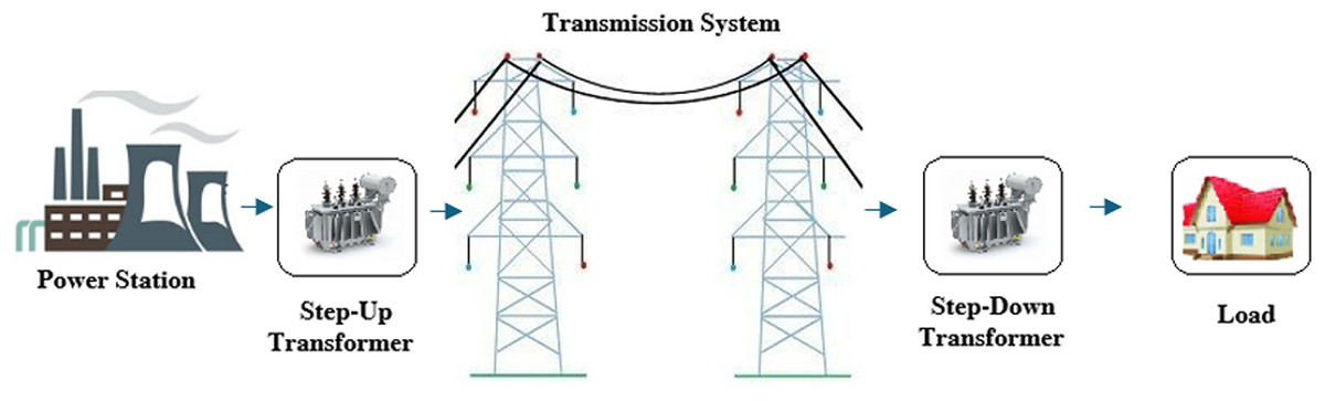
Figure 1: Simple power system infrastructure.
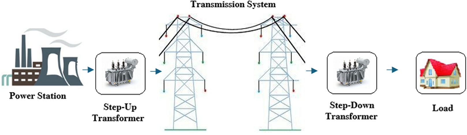
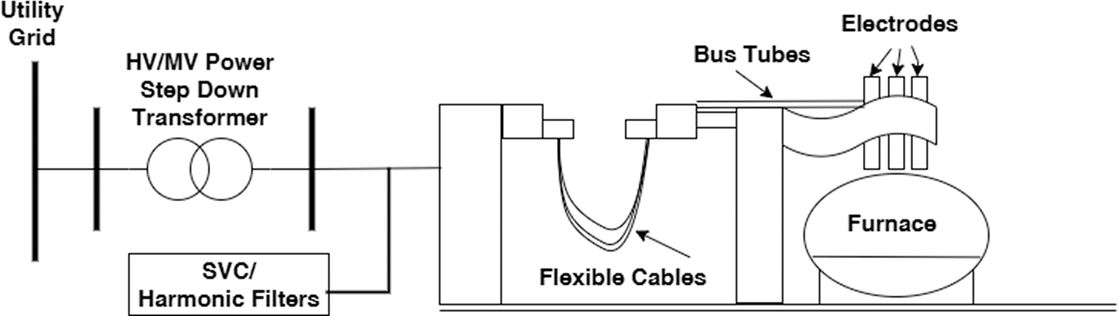
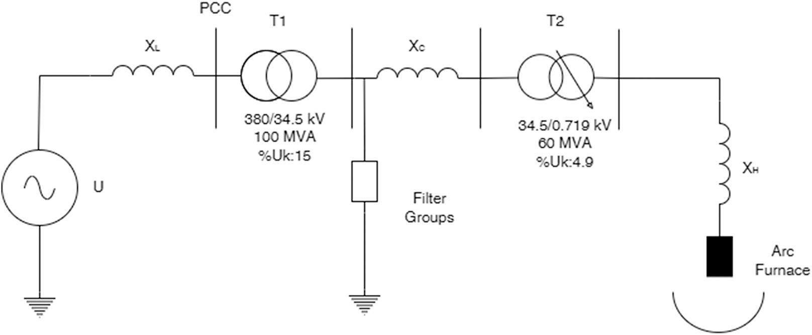
Electric arc furnaces (EAFs) (Fig. 2) provide melting by heating the material with the help of electrodes. Although the melting process may seem costly, it is more economical than other melting methods based on the unit melting amount. Electric arc furnaces are designed in various sizes from a few tons to 400 tons capacity. The temperature in these industrial furnaces can reach up to 3,300 Fo. EAFs perform the melting process with the help of the heat generated by the electrical arc formed between the electrode used and the material to be melted (Conejo, 2024). In this respect, it has a different working principle than induction furnaces. EAFs are being used more and more widely in metal melting processes due to the fact that melting can be performed at larger capacities and thus the production costs per unit are more economical (Arrillaga & Watson, 2003).
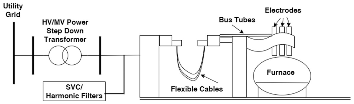
Figure 2: EAF system.
EAFs have nonlinear load characteristics. In terms of industrial applications, they can be defined as the loads with the largest nonlinear characteristics. Due to this characteristic, EAFs cause power quality problems in the networks to which they are connected. In nonlinear characteristic load structure, the current and voltage characteristic behavior has nonlinear behavior. Therefore, it is very difficult to define the relationship between current and voltage sags in such loads. In addition, as a result of these sags caused by the nonlinear load structure, systems with EAFs contain intense current and voltage harmonics (Arthur & Shanahan, 1996). Harmonics may cause irregular operation and overheating of transformers, generators and other electrical equipment connected to the grid and may cause additional losses in the system and reduce the economic life of the devices.
The most important feature that makes EAFs different from other non-linear loads is that these changes in current and voltage occur very quickly. The voltage drops caused by EAFs occur at the beginning of the melting process (during charging of the electrodes) and during the melting process. During the refining process, which is defined to keep the metal hot and not frozen during the removal of the metal after melting, no voltage collapse is observed because the metal melts and the arc length is constant. Since the voltage collapses that occur in the melting process and the resulting harmonics cause serious effects on the electricity network, the busbars to which the EAF is connected are called dirty busbars. The devices of other consumers connected to these busbars may cause serious performance degradation and failure of sensitive devices if no precautions are taken (Jones, Bowman & Lefrank, 1998).
Approximately 400 kilowatt-hours (1.44 gigajoules) or about 440 kilowatt-hours (1.6 gigajoules) per ton is required to melt one ton of steel in an EAF. Theoretically, 300 kWh (1.09 GJ) of energy is required to melt one ton of scrap steel at a melting point of 1,520 °C (2,768 °F). In 60 MVA and above arc furnaces, the total melting cycle duration, including the charging, melting, and refining phases, typically takes approximately 15 to 45 min (Chakraborty, 2013). This duration refers to the overall process time, not the data sampling interval, and represents the average time required to completely melt the intended material. Another important point to be considered here is that the regions where EAFs are planned to be installed must have a durable electrical infrastructure. The bus resistance at the point where the system is connected is generally expected to be relatively high to ensure stability. However, this is a broadly accepted design principle, and it is important to note that an optimal balance between stability and efficiency must be maintained during the system design process. In addition, in terms of the electricity intraday market, the operation of EAFs during the hours when energy costs are lower allows melting costs to be further reduced. This makes EAFs even more economical than other melting methods (Dugan et al., 2004; Arik & Pfister, 2021). Therefore, metal smelters with EAFs organize their melting strategies to take advantage of off-peak electricity prices (Gorishniy et al., 2023).
EAFs produce approximately 0.6 tons of CO2 per ton during the melting process. This value is approximately 2.9 tons in blast furnaces and basic oxygen furnaces, making EAFs more advantageous in terms of reducing CO2 emissions, which are of great importance today (Ta et al., 2023). Additionally, solving power quality issues caused by EAFs contributes to further reducing CO2 emissions indirectly by improving system efficiency. In this context, Artificial Intelligence (AI) and deep learning methods used in power quality analysis are of great importance. Deep learning models developed specifically for tables, such as the Tabular Network (TabNet), are particularly prominent in this field.
TabNet offers significant advantages in feature selection through its selective attention mechanism and can serve as a bridge between computational machine learning methods and artificial neural networks (Arik & Pfister, 2021). Some of the advantages of TabNet can be described as follows:
Feature selection: By revealing important features in the model data, the model helps us understand which features we should use in forecasting. This improves the interpretability of the model.
Interpretable model: Thanks to TabNet’s attention mechanism, it is possible to understand the data on which the model bases its decisions. This feature provides more transparency compared to other deep learning models.
Performance: TabNet is a particularly effective model for large datasets. It has similar or better performance than popular machine learning models (e.g., Extreme Gradient Boosting (XGBoost), Random Forest) on structures with many tables and datasets.
TabNet not only performs well on data but also provides interpretable models. Besides this feature, self-supervised learning methodologies can be added to TabNet. These extensions significantly increase the functionality of the method. Thus, it can increase the prediction efficiency without the need for expensive and labor-intensive large, labeled datasets. This feature gives TabNet an advantage over other traditional methods and makes it an important alternative with its solution efficiency (Arik & Pfister, 2021). It is very difficult to analyze the current and voltage variations caused by nonlinear loads such as EAFs. Using TabNet for this investigation will contribute to the creation of more understandable and usable data for researchers and professionals working in this field. Figure 3 shows the block diagram of TabNET.
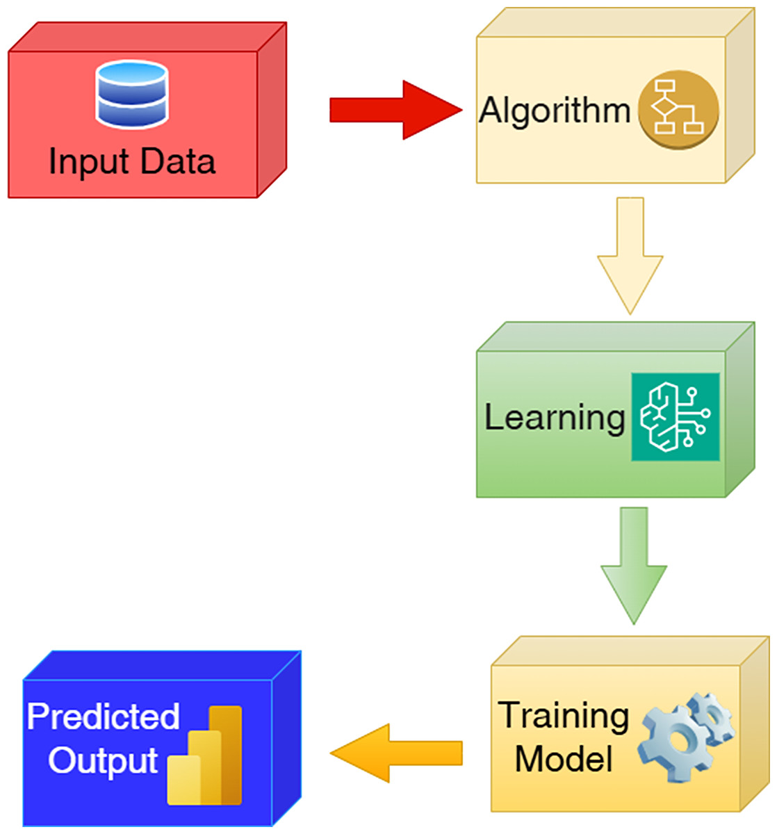
Figure 3: Schematic diagram of TabNET.
Neural Oblivious Decision Ensembles (NODE) is a model that integrates deep learning with decision trees. This model includes Oblivious Decision Trees (ODT), which use the same partition features and thresholds at each node at the same depth (Popov, Morozov & Babenko, 2019). This structure optimizes feature selection and decision-making structures at each level of the tree in the deep learning process. The main features of NODE are as follows:
Performance on datasets: NODE is efficient in analyzing both large and small datasets. It performs well on multiple datasets, especially when compared to the XGBoost method.
Gradient based optimization: This model is trained with a gradient-based optimization algorithm. This structure combines decision trees and neural networks to take advantage of the advantages of both models.
Hyperparameter tuning: NODE improves model efficiency by producing superior results, especially during hyperparameter optimization. It provides classification and regression performance on tabular datasets and automatic feature selection and robust prediction performance on comprehensive datasets.
With these features, the NODE structure offers an innovative and competitive method by combining decision trees with deep learning methodologies (Popov, Morozov & Babenko, 2019). Such models stand out as a powerful tool, especially in the analysis of complex system behavior.
In this context, harmonic currents caused by voltage drops in EAFs lead to voltage quality degradation—such as voltage imbalances and excessive currents—resulting in power quality issues. This situation brings with it many problems, such as a reduction in the economic life of equipment, deterioration of system performance, and increased energy losses. To mitigate these negative effects, harmonic filtering, compensation, and appropriate system design using different methodologies are required. However, the effective design of such a system is only possible with a good analysis of sudden changes in current and voltage—i.e., collapses. In this study, a voltage “collapse” is operationally defined as a one-cycle (50 Hz) RMS phase-voltage drop below 0.10 p.u. sustained for ≥20 ms; the event terminates when the RMS rises above 0.25 p.u. (hysteresis).
Related works
Voltage collapses in EAFs are the result of a completely nonlinear load structure and are a major power quality problem in power systems. The harmonics and flicker effects caused by this characteristic structure adversely affect the stability of the power system. The main factor in the occurrence of voltage collapses in EAFs is that the arc distance between the melted material and the electrodes changes continuously during the melting of the metal (Sharmeela et al., 2004).
EAFs also require high reactive power during operation. Due to this reactive power effect, voltage imbalances occur in the system. In addition, the reactive power effect can also cause voltage sags in sensitive power systems (Chen, Wang & Chen, 2001; Gkavanoudis & Demoulias, 2015). This asymmetric structure can increase the voltage instability and worsen voltage collapses. In some cases, the electrodes may come into contact with the molten metal. This situation creates instantaneous short circuits and negatively affects the voltage profile (Turkovskyi et al., 2020; Gkavanoudis & Demoulias, 2015).
Dynamic voltage restorers (DVRs) are used to correct voltage collapses by injecting the required voltage into the system to ensure stability. This method contributes to the improvement of power quality by effectively reducing voltage collapses (Singh & Srivastava, 2017). Different from classical compensation methods, compensation systems such as Static VAr Compensator (SVC) and STATCOM are used to reduce reactive power in EAFs. With these methods, dynamically changes the reactive power supply, effectively reducing voltage fluctuations and flicker (Chayapathi, Sharath & Anitha, 2013; Aguero, Issouribehere & Battaiotto, 2006; Sharmeela et al., 2004).
Nowadays, with the development of semiconductor technology, the application of modern control strategies can effectively ensure voltage stability and improve power quality problems (Sheng, 2008). Constant Current-Constant Voltage Converters reduce the negative effects on power quality by stabilizing the arc current and voltage. This method is particularly advantageous in small power systems and offers a cost-effective alternative to reduce voltage fluctuations (Turkovskyi et al., 2020). Zhao et al. (2006) introduced preventive control approaches including linear programming and heuristic algorithms to maintain voltage stability.
The above-mentioned methods reduce the voltage collapse problem in EAFs. However, it is very important to evaluate the cost elements of these methods in terms of applicability and to determine the most economical solution.
Deep learning models such as Recurrent Neural Networks (RNN) and Convolutional Neural Networks (CNN) provide significant benefits over traditional machine learning techniques in analyzing power grid problems. These models allow us to manage complex non-linear data models. They are also very good at capturing both temporal and spatial dependencies. The use of CNNs and RNNs in power systems contributes to increasing the reliability of problem identification and reduces the downtime. Thus, the flexibility of the system is increased. CNNs are excellent at extracting specific features from power grid data (Chen et al., 2023). RNNs, on the other hand, enable more accurate modeling of time series data by effectively capturing temporal dependencies. This advantage facilitates the prediction of future problems in power systems (Udhaya Shankar, Ram Inkollu & Nithyadevi, 2023; Xu, 2024). Deep learning models provide better accuracy in fault diagnosis and prediction compared to traditional methods. The Inception V3 model achieves a fault diagnosis accuracy of 96.7%, while Long Short-Term Memory (LSTM) models achieve 87.2% accuracy in fault prediction within 1 h (Wu, Yang & Xu, 2023).
The MCCNN-LSTM method outperforms previous deep learning models such as VGG19 and SPPD (Xu, 2024). The integration of CNNs and RNNs allows early detection and precise localization of potential problems in power systems (Chen et al., 2023). Furthermore, these models increase the durability and reliability of electrical systems by providing decision-making and efficient restoration procedures (Udhaya Shankar, Ram Inkollu & Nithyadevi, 2023).
Recent advancements in deep learning have brought Transformer-based architectures into focus for evaluating voltage stability. Li et al. (2024) proposed a Stability Assessment Transformer (StaaT) model that utilizes multi-head self-attention and conditional Wasserstein GAN-based data augmentation (CWGAN-GP) for short-term voltage stability assessment (STVSA). This model effectively addresses significant imbalances of up to one percent. Tests conducted on an IEEE 39-bus system using the proposed method demonstrate higher success rates compared to traditional deep learning algorithms, even under imbalanced and noisy load conditions (Li et al., 2023). When compared to TabNet and NODE, Transformer-based models (e.g., StaaT) capture long-term dependencies in time series voltage data more effectively, enabling more accurate assessments of system dynamics in rapidly changing conditions. TabNet offers interpretable feature selection, while NODE combines decision trees with deep learning to provide robust learning on tabular data. Transformers, on the other hand, have the advantage of directly modeling correlations over time through attention mechanisms and addressing class imbalances through synthetic sampling (Li et al., 2023). In addition, the X-WaveVT model integrates wavelet transforms, visual Transformers, and transfer learning to provide more robust voltage stability prediction with missing or noisy data. This model makes the decision process interpretable through class activation mapping (CAM) and significantly improves prediction reliability under missing data conditions, demonstrating superior performance over traditional DL models in real-time applications (Yang et al., 2025).
Although deep learning models offer significant advantages, it is important to determine what the computational complexity will be and what data will be needed. If the data structure is not well defined, it may not be possible to outperform classical methods. Therefore, incorporating deep learning into existing systems requires a rigorous assessment of infrastructure and skills to maximize its potential.
Combining deep learning models such as TabNet and NODE with decision trees has shown the potential to improve the interpretability and effectiveness of machine learning on tabular data. TabNet uses an attentional approach to identify important features, while NODE integrates deep learning with decision tree architectures to improve learning efficiency. While these models can be used to predict many problems in energy systems, in this study they are used to predict voltage collapse caused by EAFs. With this feature, the presented approaches examine for the first time the effectiveness of TabNet and NODE in the detection of voltage collapse caused by electric arc furnaces.
Feature selection: TabNet uses a sequential attention process that allows it to focus on the most relevant features at each decision point. This selective attention improves interpretability and learning efficiency by focusing the model’s capacity on prominent features (Arik & Pfister, 2021).
Sparse attention: The model uses a sparse mask to describe features, facilitating the generation of interpretable feature attributions and insights into the model’s behavior (Arik & Pfister, 2021).
Self-supervised learning: TabNet facilitates self-supervised learning and improves performance by using unlabeled data for unsupervised representation learning (Arik & Pfister, 2021).
NODE’s Oblivious Decision Trees architecture: NODE combines the hierarchical structure of deep learning using decision trees. This combination facilitates gradient-based optimization (Popov, Morozov & Babenko, 2019).
NODE has proven its effectiveness in managing tabular data by outperforming traditional gradient boosting decision trees (GBDT) on multiple tabular datasets (Popov, Morozov & Babenko, 2019).
DL techniques such as neural networks and decision trees can be used to assess voltage stability in power systems. These models facilitate the prediction of voltage collapse (Onah et al., 2024) through the analysis of stability indices and related characteristics to be defined (Choudekar, Asija & Ruchira, 2017).
In recent studies such as Mollaiee et al. (2021) and Voropai et al. (2018), a combination of data sampling, dimension reduction, feature selection, and machine learning model optimisation has been used to improve voltage stability assessment in power systems (Mollaiee et al., 2021; Voropai et al., 2018). Voltage failure in the Nigerian 330kV transmission network was effectively predicted (Onah et al., 2024).
The emergence of different load structures in power systems over time (such as renewable energy sources and electric vehicles …) increases data complexity and the need for real-time data processing. Therefore, new models and interpretation techniques need to be continuously improved to make the system understandable. Despite the significant progress made by TabNet and NODE in managing table data, especially in power systems, problems remain. The inclusion of different loads changes the dynamics of the system. Therefore, it is necessary to develop flexible and applicable machine learning models (Alimi, Ouahada & Abu-Mahfouz, 2020).
Methodology
In this study, the TabNet and NODE models are utilized for the Arc Furnace Dataset.
TabNet is a unique deep learning architecture developed specifically for processing tabular data. This structure can identify relationships between important features and improve prediction accuracy thanks to sequential attention mechanisms. The model processes input data through a series of decision steps, with two main components performing tasks at each step: feature transformer and attention transformer.
The feature transformer component converts the data into higher-dimensional representations, enabling the model to learn complex patterns. This process utilizes dense neural network layers and non-linear activation functions. The transformed data is then passed to the attention transformer component. This module produces an attention mask using attention scores to determine the most relevant features at each decision step.
Thanks to a special sparsification mechanism within the model, TabNet focuses only on the most relevant information. This selective learning approach improves both the model’s performance and its interpretability.
NODE is another deep learning model specifically designed for tabular data. This model utilizes differentiable ODTs as its base structure. In the NODE model’s inner structure, each ODT consists of a binary decision tree with fixed splits that are applied to input features, which enables both parallel computation and gradient-based optimization. The NODE model includes multiple ODTs in an ensemble structure, where each tree contributes to the final prediction. Unlike traditional decision tree ensembles, NODE optimizes its structure through backpropagation by integrating the strengths of both neural networks and tree-based methods.
The main advantage of the NODE model is the model’s ability to combine the interpretability of tree-based models and the optimization capabilities of neural networks. This combination enables the NODE model to be especially effective in tabular datasets with complex feature dependencies and non-linear relationships. Therefore, the NODE model’s ensemble structure provides robustness against overfitting and improves generalization by leveraging diverse representations learned by individual trees.
Dataset and features
To obtain the dataset used in this study, a one-phase equivalent circuit model of the system feeding the EAF-60 furnace in the Sivas Iron and Steel plant has been modeled in a Matlab/Simulink environment. The basic circuit elements of the system feeding the EAF-60 furnace used in the modeling are shown in Fig. 2 and the one-phase equivalent model of these circuit elements is shown in Fig. 4. In this system, one-phase equivalent circuit parameters calculated according to the reference voltage of 719 volts using the calculation parameters presented in references (Seker & Memmedov, 2017, Şeker & Memmedov, 2014; Seker, Memmedov & Huseyinov, 2017) are presented in Table 1. In this table, the parameter denoted as ‘arc impedance’ refers solely to the electrode impedance, as the impedance of the flexible cables has been neglected in the calculations due to its negligible contribution to the total series impedance of the high-current circuit.
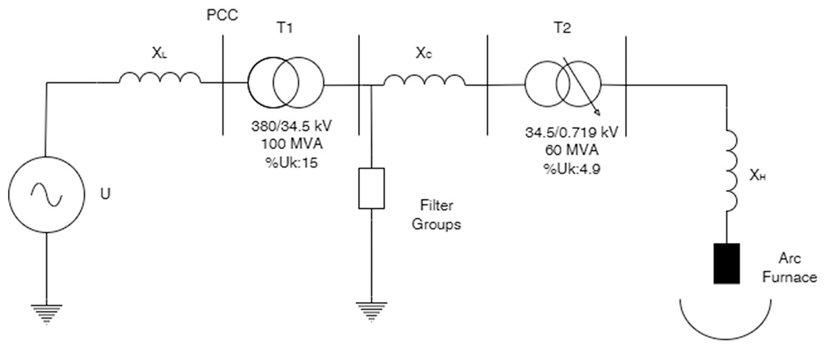
Figure 4: Single phase equivalent electrical circuit of EAF.
| Element | R (mΩ) | Jx (mH) |
|---|---|---|
| Utility line | 0.071 | 0.027 |
| Step-down transformer | 0.096 | 2.469 |
| Line (Between T1-T2) | 0.004 | 0.010 |
| EAF transformer | 0.527 | 1.343 |
| Arc impedance | 0.612 | 12.67 |
The most important issue in modeling the characteristic behavior of the EAF furnace is the modeling of the electrical arc. The Cassie-Marie method is widely used in modeling electric arcs. Cassie-Marie provides a two-region representation consistent with changes observed in real-time arc events in EAFs. The Exponential-Hyperbolic model can be described as a complementary mathematical approach to the Cassie-Marie method. This method is expressed as the temporal and polarity-dependent variation of voltage and captures the asymmetry between the rising and falling current phases (Xu, Ma & Zhang, 2022). Equations (1) and (2), although primarily derived from experimental V-I characteristics and arc length dependence, exhibit strong conceptual consistency with the Cassie-Marie model in representing arc hysteresis. In particular, the exponential form for the decreasing current and the hyperbolic response for the increasing current in Eq. (1) reflect the asymmetric arc behavior of the Cassie-Marie framework during current rise and fall. Additionally, the arc length-dependent threshold voltage defined in Eq. (2) is consistent with the representation of dynamic arc impedance and voltage thresholds under varying electrode positions in the Cassie-Marie model. The inclusion of Cassie-Marie principles provides better compatibility with power quality analysis, as it more accurately reflects the nonlinear and discontinuous harmonic injection behavior of EAF arcs (Panoiu & Panoiu, 2024). Therefore, their use together with Eqs. (1) and (2) provides a hybrid framework that balances mathematical tractability with physical realism (Klimas & Grabowski, 2024).
In this study, the Exponential-Hyperbolic model was adopted to mathematically characterize the behavior of the electric arc. The applicability and accuracy of this model have been validated through experimental measurements and simulation-based analyses in previous studies (Samet et al., 2023; Seker et al., 2017, Bhonsle & Kelkar, 2016, Şeker et al., 2025). In this model, the V-I characteristic structure of the electric arc is expressed as a hyperbolic function for increasing current and as an exponential function for decreasing current. The general mathematical expression of this approach is defined by Eq. (1) (Şeker & Memmedov, 2014).
(1)
In the exponential-hyperbolic model, the variables are defined as V(i)- arc voltage as a function of current, i- arc current, C and D are model parameters corresponding to the current’s rising (i) slope, is defining as minimum current level to starting the melting process, which should be approximately 5 kA. To represent the negative regions of the current waveform, the sign(i) function is multiplied by the mathematical expressions given in Eq. (1). This allows the model to symmetrically represent both the positive and negative directions of the current and to accurately reflect the full-cycle behavior of the arc current. This model captures the arc’s nonlinear voltage-current characteristics by distinguishing between different rates of change in arc current. By separately modelling the behaviour during the increasing and decreasing phases of the current, the exponential-hyperbolic model provides a more realistic representation of arc dynamics, particularly under transient conditions such as the melting stage in EAF operation.
In this expression, Vat is the threshold voltage, and this voltage varies depending on the arc length. Especially in the melting process, the arc length also varies due to the continuous change in the distance between the electrodes and the scrap or the melted metal. The mathematical expression of the threshold voltage depending on the variation of the arc length is expressed by Eq. (2) (Dasgupta, Nath & Das, 2012).
(2)
In Eq. (2), the A value is a constant defined by the anode and cathode voltage collapse and is assumed to be approximately 40 V. B is voltage-dependent on the arc length and is empirically assumed to be B = 10 V per cm of arc length, and l- is the length of the arc.
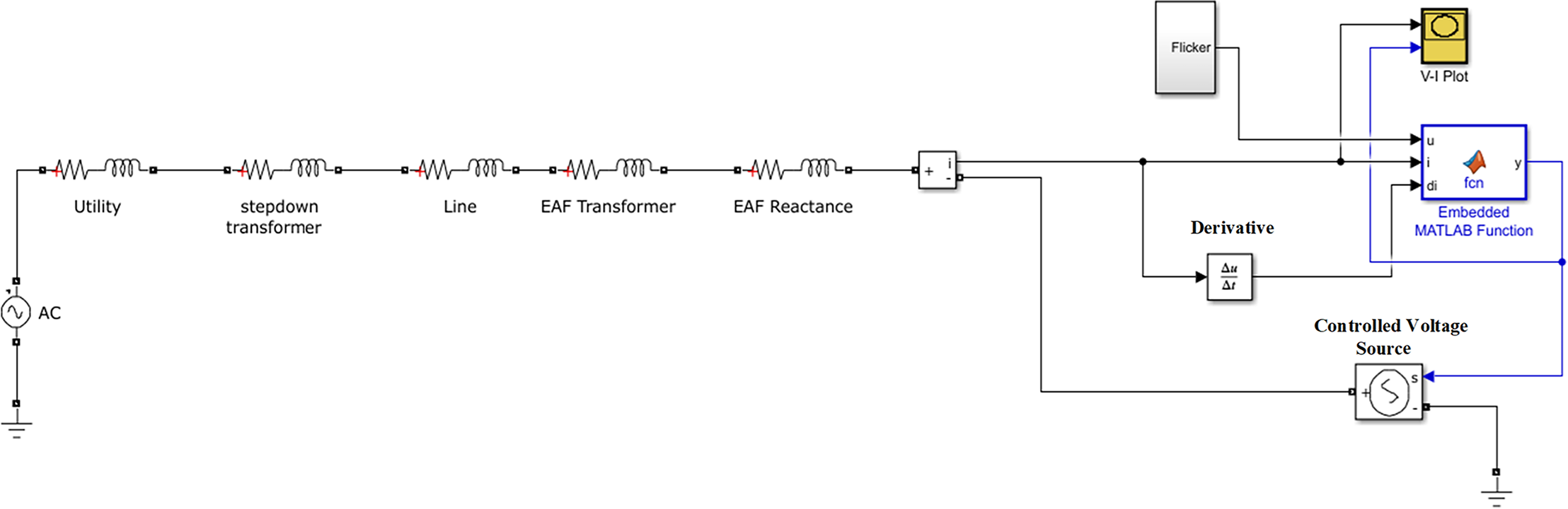
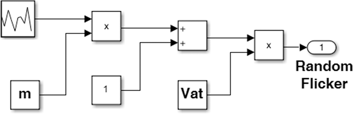
According to the mathematical assumptions mentioned above, a one-phase equivalent circuit model of the 60 MVA EAF system was created using MATLAB/Simulink as shown in Fig. 5. In this model, Eq. (3) is defined in the function block and the electrical arc is modeled using a voltage-controlled voltage source. The block structure presented in Fig. 6 is used to define the flicker effect in the system. In this block structure, the modulation index m and the threshold voltage Vat which depends on arc length are used. The Vat value is randomly varied between 0 and 240 volts to simulate the “tidal drops in the electrical system.”
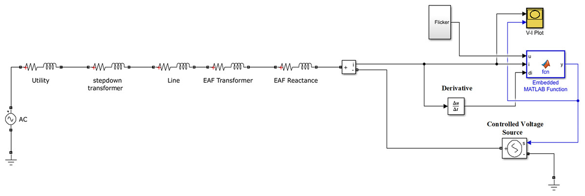
Figure 5: Single phase equivalent electrical circuit of EAF for the simulation model.
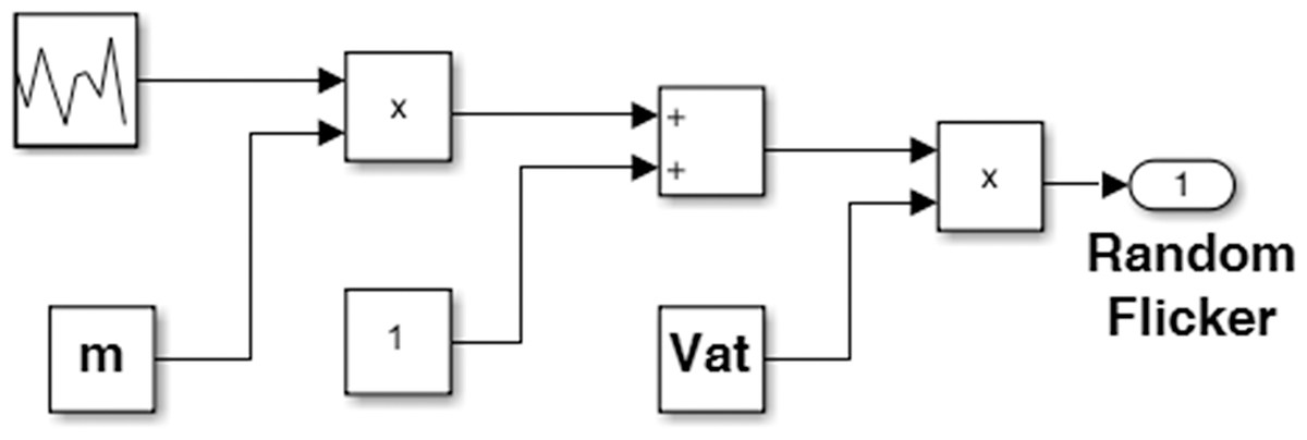
Figure 6: Block structure for defining flicker and voltage sag.
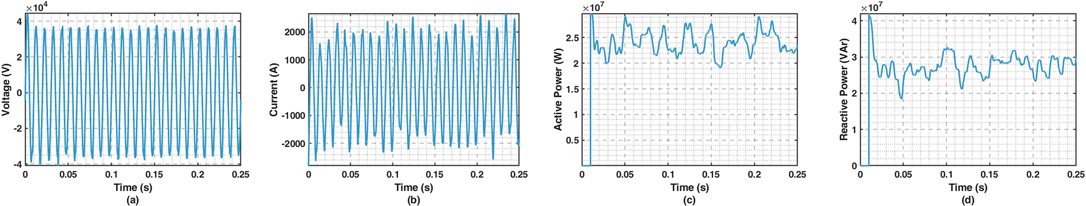
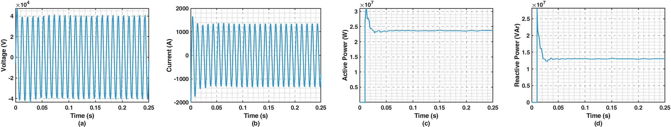
As a result of the simulation, the current (I), voltage (V), active power (P), and reactive power (Q) values at the input of the EAF transformer were recorded. In the case of no voltage collapse, the threshold voltage remains constant, and, in the simulation, it is assumed that Vat is 240 volts and does not change to define the case where there is no voltage collapse. Thus, it was attempted to classify the cases with and without voltage collapse. The variations in current, voltage, active power, and reactive power under conditions with and without voltage collapse are presented visually in Figs. 7 and 8, respectively.
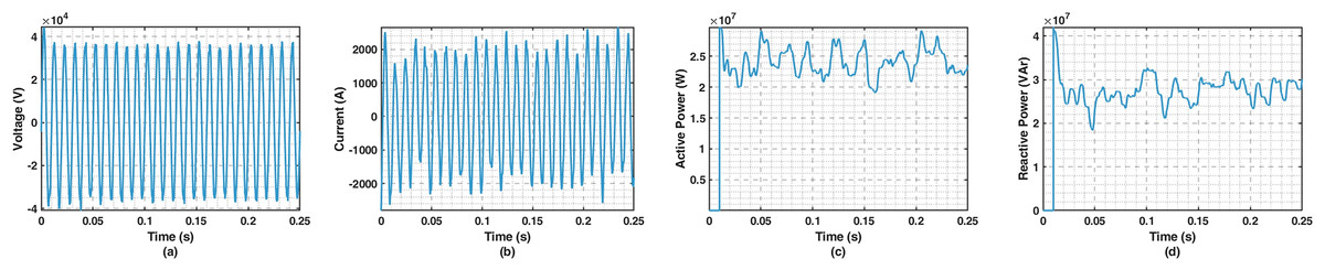
Figure 7: Simulated voltage, current, active power, and reactive power changes in the EAF melting process (variable arc length).
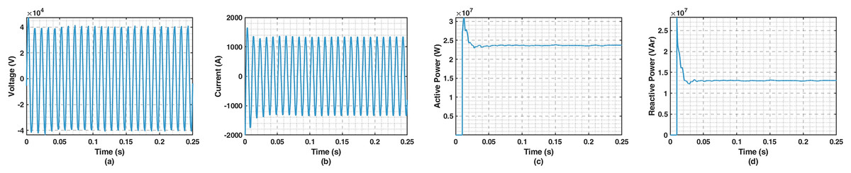
Figure 8: Simulated voltage, current, active power, and reactive power changes without the EAF melting process (constant arc length).
For experiments, we utilize the Arc Furnace Dataset, which includes specific features from three multiple phases. For determining the voltage collapse case in the samples, utilization of one specific phase is required and sufficient among multiple phases. Consequently, in the experiments, because the first phase features in the dataset (‘I1’, ’P1’, ‘Q1’, and ‘V1’) provide the most distinguishing characteristics for the voltage collapse detection by far compared to the other phase, we decided to use the first phase on the dataset for our experiments. These parameters (‘I1’, ‘P1’, ‘Q1’, and ‘V1’) represent the electrical quantities current, active power, reactive power, and voltage of the first phase and were obtained from the equivalent single-phase circuit model used in the simulation setup, as illustrated in Fig. 6.
Firstly, in the dataset, the ‘I1’ feature represents the current in the electric arc furnace circuit, which is measured in amperes (A). In the arc furnace, current fluctuations play a critical role in determining the stability of the system, because of that high or unstable currents can lead to voltage instability or collapse. Hence, the ‘I1’ feature can be counted as one of the potential indicators for the voltage collapse state because of its strong correlation with electrical instability.
The ‘P1’ feature represents the active power, which is measured in watts (W) megawatts (MW). More specifically, active power can be assumed as the portion of electrical power that performs useful work, such as heating or melting materials in the arc furnace. Again, this feature can be thought of as a potential factor for determining voltage collapse.
Additionally, the ‘Q1’ feature represents the reactive power in the arc furnace, which is measured in volt-amperes reactive (VAR). This feature is related to maintaining voltage levels in the furnace system and is not a direct factor contributing to the performing process. It helps in magnetizing devices like transformers or compensating for phase differences in alternating current.
Also, the ‘V1’ feature is the voltage in the circuit, which is measured in volts (V). Voltage fluctuations can be thought of as another potential indicator of system stability. A significant voltage drop is a critical failure mode in electric arc furnaces and electrical networks.
Lastly, ‘Collapse’ is the dataset’s target feature, which represents the occurrence of a voltage collapse condition. The feature is composed of binary values, in which the ‘0’ value means there is no voltage collapse situation, and the ‘1’ value represents the voltage collapse case.
Table 2 introduces different feature-based statistics for the Arc Furnace dataset. According to statistics, the dataset includes 9,792 samples (dataset sample size) there is no missing value case for the features of the dataset. Also, as an important observation, the target feature ‘Collapse’ has a mean and standard deviation of 0.5, which means that the dataset has balanced samples for two classes (0 and 1) and there is no class imbalance problem.
| I1 | P1 | Q1 | V1 | Collapse | |
|---|---|---|---|---|---|
| Count | 9,792 | 9,792 | 9,792 | 9,792 | 9,792 |
| Mean | 6.28 | 24,113,900.07 | 27,530,389.87 | −7.26 | 0.50 |
| Std | 1,459.33 | 2,222,373.48 | 3,120,111.82 | 25,735.02 | 0.50 |
| Min | −2,621.37 | 19,121,103.45 | 18,400,030.42 | −40,951.62 | 0.00 |
| 25% | −1,372.43 | 22,475,705.28 | 25,742,957.10 | −25,417.88 | 0.00 |
| 50% | −2.40 | 23,788,647.76 | 27,521,145.20 | −53.30 | 0.50 |
| 75% | 1,402.69 | 25,686,622.92 | 29,267,438.15 | 25,511.77 | 1.00 |
| Max | 3,052.23 | 29,725,730.42 | 42,027,693.32 | 37,932.56 | 1.00 |
The ‘I1’ feature shows a large range and significant variation of values, which can be noticed from the rather high standard deviation value compared to the mean value of the respective feature in Table 1. It can be also observed that the feature contains negative values, which can be concluded as reverse or reactive current conditions.
The ‘P1’ feature has relatively less variation compared to its mean value, which indicates a stable power factor. Additionally, in the feature, the values are all observed to be positive, which points out consistent active power consumption.
The ‘Q1’ feature includes more variation than the ‘P1’ feature, because of has a higher standard deviation relative to its mean value, which can be interpreted as potential fluctuations for reactive power demand.
Finally, the ‘V1’ feature has a mean close to zero value but also shows very high variation with the extreme range of positive and negative values. Consequently, this observation can be concluded as significant voltage fluctuation, which means that this feature has a high potential factor for effect on voltage collapse behavior.
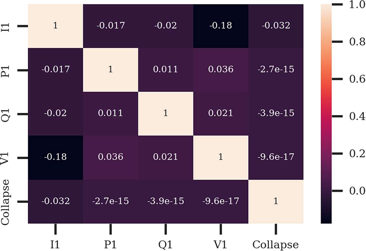
Figure 9 represents the correlation heat map showing the linear correlation levels among phase 1 features (‘I1’,’ P1’, ‘Q1’,’ V1’) and target feature ‘Collapse’. An important observation is that there are no significant linear correlations between any input phase 1 feature and with ‘Collapse’ feature, which demonstrates the target feature relies on non-linear or complex relationships among features rather than linear relationships. Additionally, there is no strong correlation between any of the input features, which points out that the input features have the potential to contribute independently to the target feature.
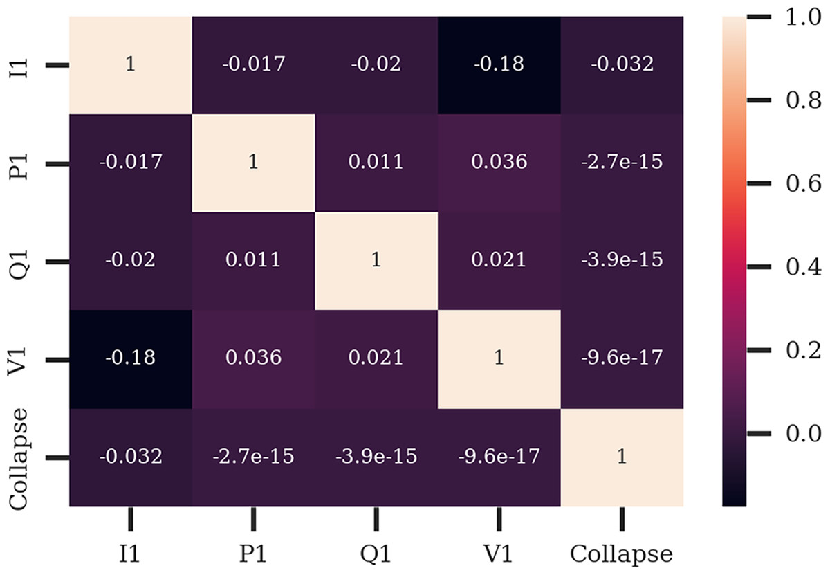
Figure 9: Correlation heat map for the phase 1 features (I1, P1, Q1, V1) and target feature ‘Collapse’ for Arc Furnace dataset.
Because of that the individual value range of the dataset features is highly variational, an additional min-max normalization process is applied to each feature of the dataset with the formula below:
(3) where X represents normal values of the specific feature and X′ represents the new values of the same feature. Additionally, Xmax represents the maximum value within the feature’s values and similarly Xmin represents the minimum value within the feature’s values. Consequently, this process enables every feature’s range to be set as (0–1) range and each feature’s value range is the same, therefore the model shows equal importance to the features in the training process.
Utilized models
Inner architecture of TabNet model: The architecture of TabNet includes a series of sequential decision steps processing the input data iteratively. Each decision step contains two main components, which are the feature transformer and the attentive transformer modules. The feature transformer module transforms the input features into higher-dimensional representations. It deploys dense neural layers with nonlinear activation functions to leverage the model to learn complex patterns in the data. These transformed features are consequently passed into the attentive transformer, which focuses on the most relevant features by comparing them selectively.
The attentive transformer module also calculates a particular attention mask by using a sparse mechanism with learned weights. This specific mask prioritizes which features are important at a given decision step, which enables the model to focus its learning efforts on relevant and key aspects of the dataset. This module is also regulated by a particular sparsity constraint, which forces the model to use only a subset of the available features at each step. This procedure not only enhances the interpretability of the model but also prevents overfitting by reducing the dependence on irrelevant features.
A critical advantage of TabNet is the model’s entirely differentiable pipeline, which provides end-to-end optimization through the gradient descent method. Additionally, TabNet incorporates a self-supervised learning phase, where the model is trained on unlabeled data to learn meaningful feature representations. This capability is especially advantageous in cases where labeled data is scarce, because of enables the model to leverage the underlying structure of the data before fine-tuning the supervised task.
Inner architecture of NODE model: The architecture of the NODE model consists of specific tree-based structures called ODT, which is a specialized type of decision tree where each internal node conducts the same splitting condition for all samples in the dataset. Unlike traditional decision trees, which dynamically decide split criteria at each node, ODTs operate on fixed decision boundaries for the entire dataset. This uniformity enables both parallelized computations and suitable integration with gradient-based optimization techniques.
The NODE model is composed of an ensemble of multiple ODTs, which forms again an interpretable model capable of capturing intrinsic feature relationships. Each tree in the ensemble learns a distinct representation of the data, which further leverages the overall estimation process by aggregating outputs through a weighted averaging mechanism. The weights for each tree are learned during training, which provides the NODE model to balance the contributions of individual trees dynamically.
The NODE model also utilizes an end to end differentiable pipeline by processing the entire ensemble as a differentiable computational graph. This end-to-end differentiability process enables the NODE model to leverage the gradient descent to optimize its parameters, unlike traditional tree-based methods that rely on heuristic-based optimization.
Model selection and hyperparameter optimization: For the experiments, the dataset is split into training, validation and test sets. Training set is used for the training process of the models, while validation set is used for the specific fine-tuning techniques such as hyperparameter optimization or early stopping for the models. Finally, the test is utilized for comparing models’ estimations and target (ground-truth) values by using specific performance metrics.
Respectively, Accuracy, Precision, Recall and F1-score performance metrics are utilized for this study as the detection of voltage collapsing task is assumed as binary classification task within this study.
The reason for utilization of additional metrics (Precision, Recall and F1-score) in addition to accuracy metric is that accuracy alone is insufficient, as it does not differentiate between false positives and false negatives within the dataset. Precision metric helps for evaluating the reliability of collapse predictions by reducing unnecessary alerts, while recall metric ensures that the model captures all critical collapse events for preventing system failures. Finally, F1-score is a balanced metric for the trade-off between precision and recall, which makes it ideal for evaluating models in scenarios where both false positives and false negatives have important effects.
Experimental results
For the experiments, training, validation and test sets are adjusted as 80%, 10% and 10% from the whole dataset and shuffling process is applied before dividing process, for balanced sample distribution. Additionally, for quantitative analysis, TabNet and NODE models are also compared with XGBoost, Random Forest and Support Vector Machine (SVM) models. Finally, TabNet and NODE models are also analyzed with two Explainable AI (XAI) approaches which are SHapley Additive exPlanations (SHAP) and Local Interpretable Model-agnostic Explanations (LIME) and compared with their feature importance and other specific SHAP and LIME figures through global and local level explanations.
As for parameter settings, TabNet and NODE models are run with their default parameter settings and for both TabNet and NODE models we use batch size as 50 and max epoch size as 50. We additionally use early stopping approach for TabNet and NODE models in the validation set to prevent overfitting issue. Also, the XGBoost model estimator number is set to 2 and the logistic objective function is used. Random Forest model’s estimator number is also set to 2 and finally, SVM model’s ‘C’ parameter is set as 1.0 and radial basis function is used as kernel function.
Performance comparison
Table 3 shows the obtained class-based Precision, Recall, F1-score and Accuracy (Overall for all two classes) metric performances on the test set for TabNet, NODE, Random Forest, SVM and XGBoost models. Also, ‘Support’ metric represents the respective sample count for each class (0 and 1). Consequently, for each model compared, we can observe that sample distributions for each class are nearly balanced.
| Class | Precision | Recall | F1-score | Accuracy | Support | |
|---|---|---|---|---|---|---|
| TabNet | 0 | 0.99 | 0.92 | 0.95 | 0.95 | 506 |
| 1 | 0.92 | 0.99 | 0.95 | 474 | ||
| NODE | 0 | 1.00 | 0.90 | 0.95 | 0.95 | 506 |
| 1 | 0.91 | 1.00 | 0.95 | 474 | ||
| Random forest | 0 | 0.89 | 0.97 | 0.93 | 0.92 | 506 |
| 1 | 0.96 | 0.87 | 0.91 | 474 | ||
| SVM | 0 | 1.00 | 0.82 | 0.90 | 0.91 | 506 |
| 1 | 0.84 | 1.00 | 0.91 | 474 | ||
| XGBoost | 0 | 0.98 | 0.80 | 0.88 | 0.89 | 506 |
| 1 | 0.82 | 0.98 | 0.89 | 474 | ||
| TabNet (I1, V1) | 0 | 0.99 | 0.92 | 0.95 | 0.95 | 506 |
| 1 | 0.92 | 0.99 | 0.95 | 474 | ||
| NODE (I1, V1) | 0 | 1.00 | 0.90 | 0.94 | 0.94 | 506 |
| 1 | 0.90 | 1.00 | 0.95 | 474 |
Analysis of results
Firstly, the TabNet model achieves 0.95 accuracy value, which means the high overall performance and the model effectively learns the complex relationships in the dataset. Additionally, we can observe that the model performs equally well for both classes, as indicated by the identical F1-scores for Class 0 and Class 1. This is particularly important for situations where both classes are equally critical, such as voltage collapse prediction in our study. Finally, the recall value of 0.99 for Class 1 ensures that almost all instances of voltage collapse are identified, which minimizes the risk of missing critical voltage collapsing events.
The NODE model shows again a strong level of overall accuracy with 0.95 value, which demonstrates again the NODE model’s representation performance of relationships between the input features. Also, the precision of 1.00 for Class 0 for the NODE model means there are no false positives, which is vital in scenarios where misclassifying a non-collapse event as a collapse could lead to unnecessary interventions. Additionally, the recall of 1.00 for Class 1 ensures that the model correctly assumes all instances of voltage collapse, which again minimizes the risk of missing critical events. Ultimately, with identical F1-scores (0.95) for both classes, NODE shows strong and balanced performance, which makes it reliable for conditions with equal importance for both classes.
From Table 3, we can also conclude that both TabNet and NODE models outperform Random Forest in overall accuracy, recall for Class 1, and F1-scores for both classes. Their advanced architecture allows for better handling of complex feature interactions and non-linear relationships in the dataset. On the other hand, we can observe that Random Forest model excels in recall for Class 0 and precision for Class 1. Ultimately, while Random Forest model is a simpler and interpretable alternative, TabNet and NODE models remain the preferred models for voltage collapse prediction in the Arc Furnace Dataset, especially for high-risk scenarios requiring consistent and accurate predictions across all classes.
Again, in Table 3, the SVM model demonstrates a rather strong performance with an accuracy of 91%, perfect precision for Class 0, and perfect recall for Class 1. However, it struggles with lower recall for Class 0 and overall balance, which makes it less effective than TabNet and NODE models (Both achieving 95% accuracy and F1-scores of 0.95 for both classes). While SVM has specific strengths, particularly for minimizing false positives for no-collapse predictions and detecting all collapse instances, TabNet and NODE models again remain the preferred models for voltage collapse prediction in the Arc Furnace dataset by showing superior and more consistent performance across overall.
Ultimately, in Table 3, the XGBoost model demonstrates comparable performance in voltage collapse prediction but falls short of the superior accuracy and balanced metrics achieved by TabNet and NODE models. While XGBoost model excels in precision for Class 0 and recall for Class 1, it struggles with recall for Class 0 and overall balance, which makes it less suitable for applications requiring high overall accuracy. On the other hand, TabNet and NODE models, with their advanced architecture and interpretability, remain the preferred models for this dataset by offering robust and balanced performance across overall metrics.
Model interpretability and transparence
According to the results of Table 3, we select our best overall performed models as TabNet and NODE models and introduce the SHAP and LIME based experiments and feature importance and interpretability analyzes for these two models, globally and locally.
SHAP and LIME results for the TabNet model
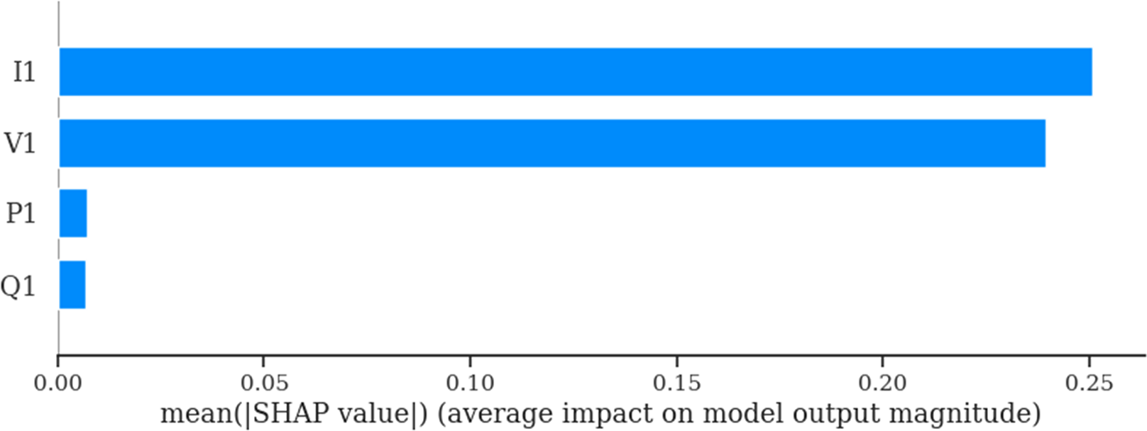
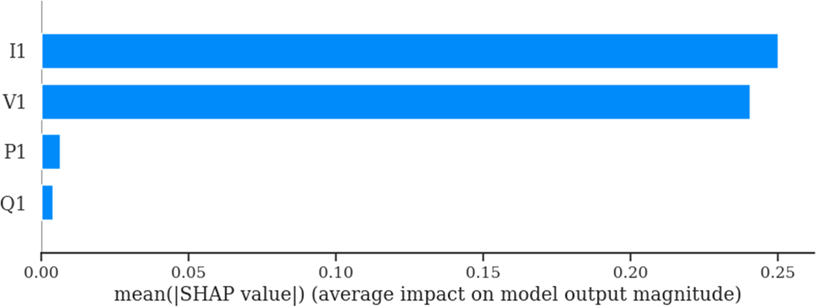
The SHAP based bar plot (Fig. 10) shows that TabNet model’s predictions are primarily influenced by ‘I1’ (current) and ‘V1’ (voltage) features, which makes them the most relevant features for predicting voltage collapse for TabNet model. The minimal influence of ‘P1’ (active power) and ‘Q1’ (reactive power) also indicates that these features do not play an important role in the TabNet model’s decision-making process.

Figure 10: SHAP bar plot for TabNet model.
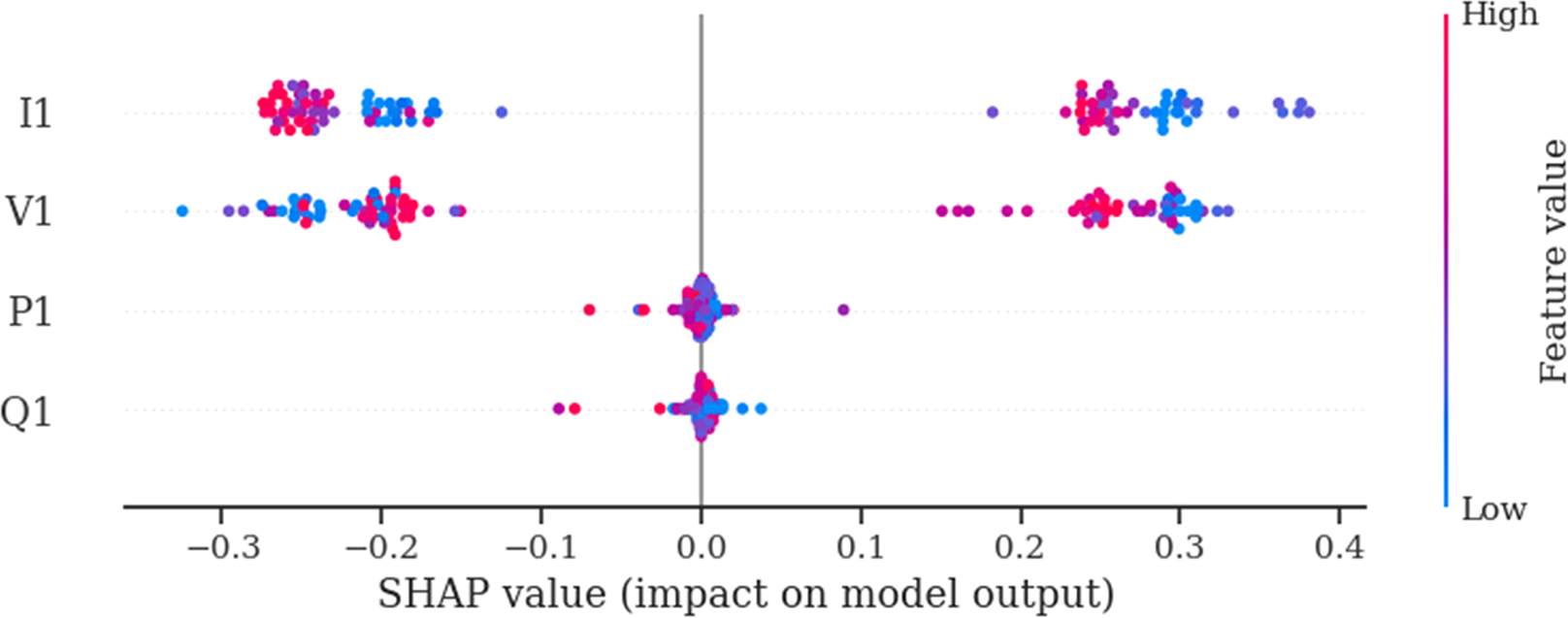
The SHAP summary plot (Fig. 11) reaffirms that ‘I1’ (current) and ‘V1’ (voltage) are the most influential features for affecting the TabNet model’s predictions for voltage collapse. These features exhibit strong and dynamic relationships with the target variable, while P1 (active power) and Q1 (reactive power) play minimal roles. This SHAP based summary plot analysis confirms the model’s ability to prioritize the most relevant features and capture non-linear interactions, which makes it a robust tool for predicting voltage collapse in the Arc Furnace dataset.
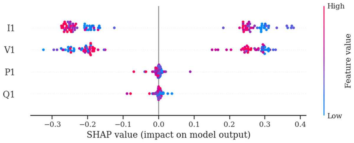
Figure 11: SHAP summary plot for the TabNet model.
The SHAP decision plot (Fig. 12) also confirms that ‘I1’ (current) and ‘V1’ (voltage) are the most important features in the TabNet model’s estimations for voltage collapse. These features again show vital contributions, with high values driving predictions toward collapse and low values pushing predictions away from collapse. The minimal impact of ‘P1’ (active power) and ‘Q1’ (reactive power) again in this figure reinforces their limited role in the TabNet model. Overall, the decision plot again confirms the TabNet model’s ability to effectively capture the non-linear interactions between key features and the target variable.
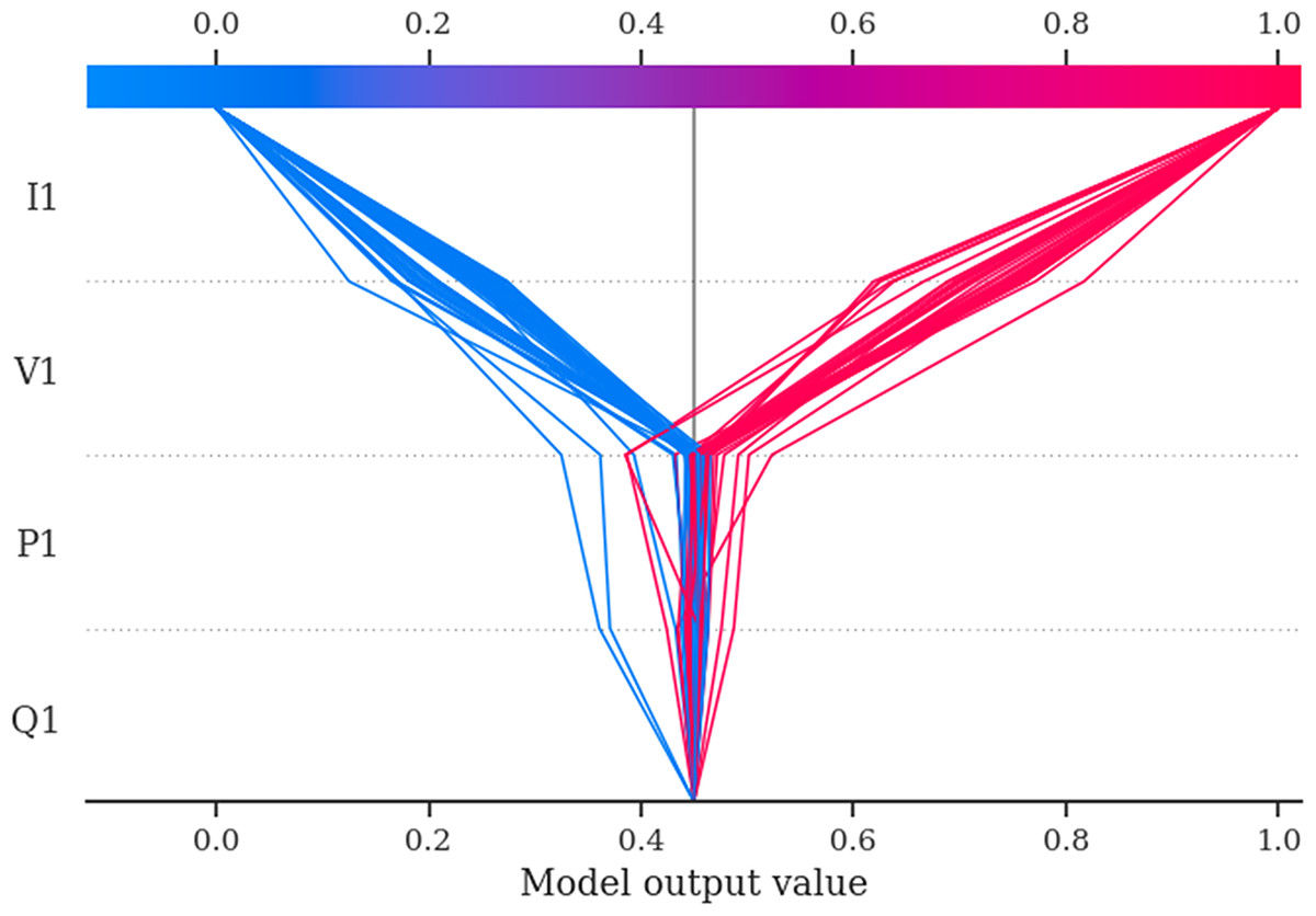
Figure 12: SHAP decision plot for the TabNet model.
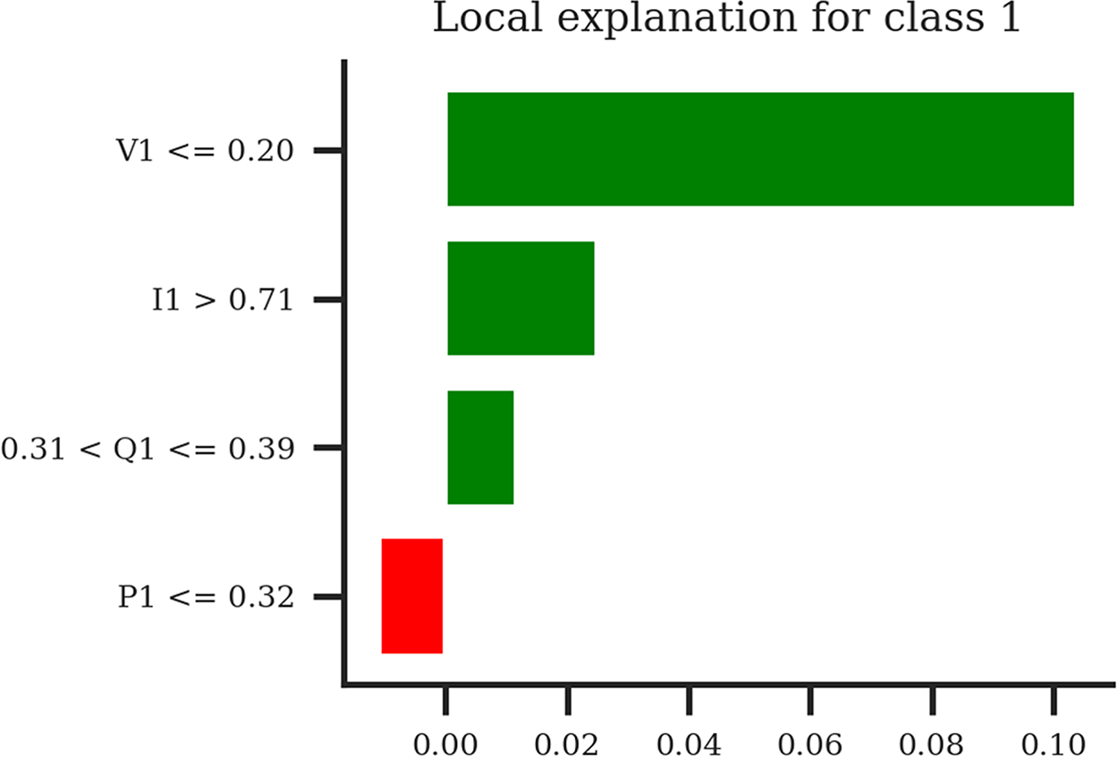
The LIME bar plot for the particular sample (Fig. 13) reveals again that low voltage (V1 <= 0.20) and high current (I1 > 0.71) are the primary factors of the TabNet model’s prediction for voltage collapse in this sample. Additionally, reactive power (Q1) has a minor positive impact, while active power (P1) slightly contradicts the collapse prediction. This localized explanation also indicates the transparency of the TabNet model and provides insights into the feature contributions for individual prediction for TabNet model.
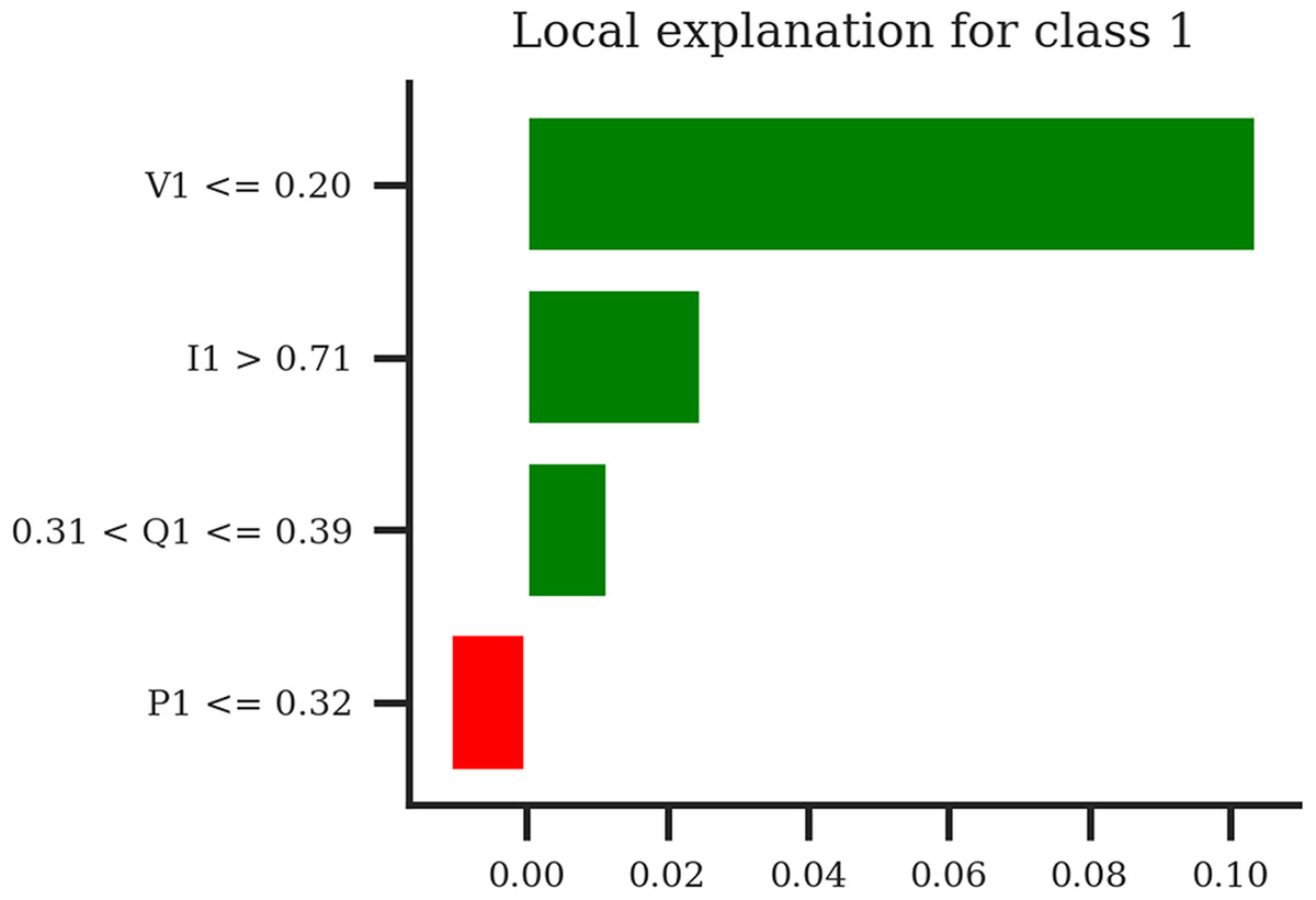
Figure 13: LIME bar plot for the TabNet model for specific sample.
The LIME prediction plot (Fig. 14) again points out that the TabNet model’s prediction for this sample is primarily driven by the extremely low voltage (V1 = 0.06) and followed by the high current (I1 = 0.90). Reactive power (Q1) and active power (P1) affect minimally to the prediction. Consequently, the model demonstrates a clear and interpretable decision-making process, which aligns with domain-specific knowledge of voltage collapse phenomena. This transparency further reinforces trust in the model’s predictions and provides additional insights for managing electrical stability in Arc Furnace systems.
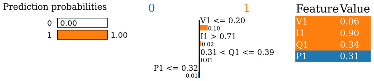
Figure 14: LIME prediction plot for the TabNet model for specific sample.
SHAP and LIME results for the NODE model
The SHAP bar plot (Fig. 15) highlights again that the NODE model’s predictions are primarily influenced by I1 (current) and V1 (voltage), while P1 (active power) and Q1 (reactive power) affect minimally for the model’s estimation. This result further aligns with the TabNet Model’s respective SHAP bat plot result. And also this result indicates that the NODE model effectively identifies and prioritizes the most critical features, making it a reliable and interpretable tool for voltage collapse prediction in the Arc Furnace dataset.
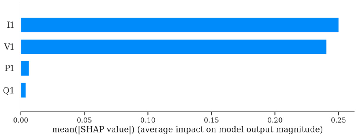
Figure 15: SHAP bar plot for the NODE model.
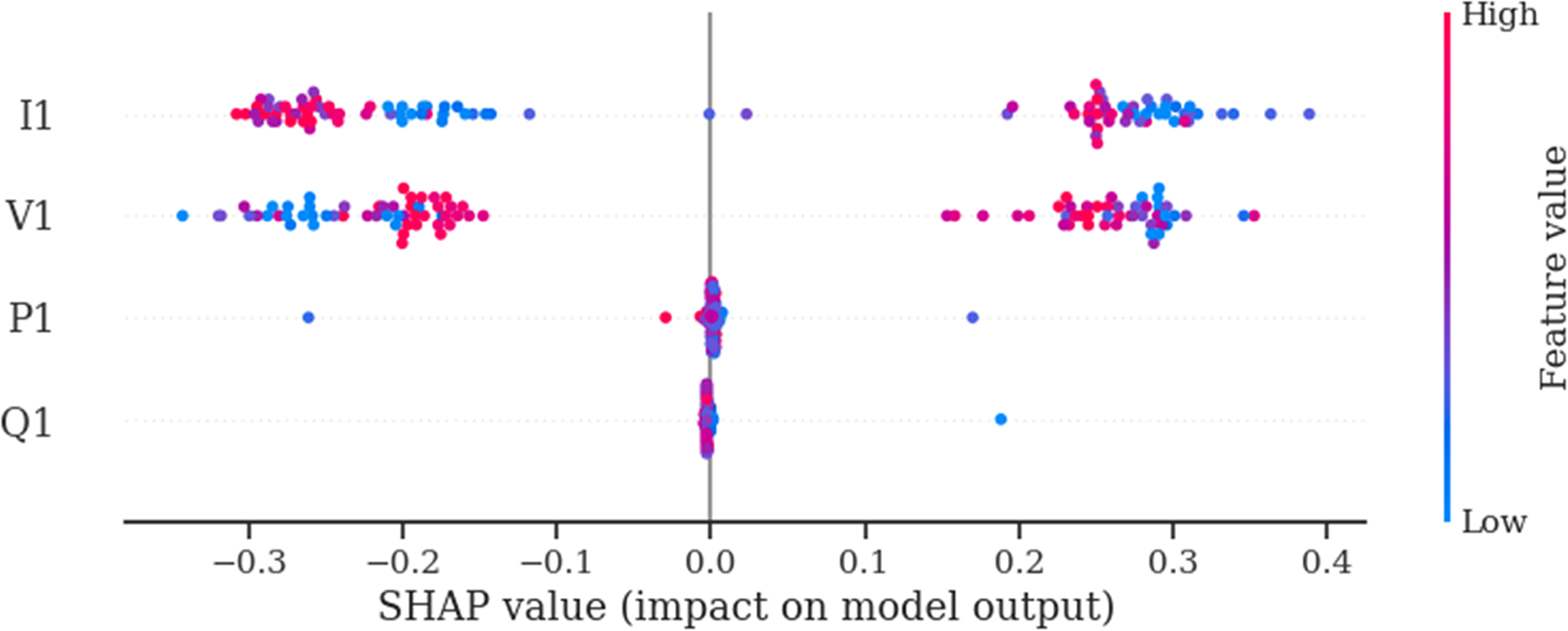
The SHAP summary plot (Fig. 16) again confirms that the NODE model’s predictions are mainly driven by I1 (current) and V1 (voltage), with minimal contributions from P1 (active power) and Q1 (reactive power). Consequently, this result shows that the model effectively captures the non-linear relationships between these features and the target variable (Collapse), which demonstrates its robustness and alignment with domain-specific knowledge. This observation additionally supports the importance of focusing on I1 and V1 for accurate and reliable voltage collapse prediction in the Arc Furnace dataset.
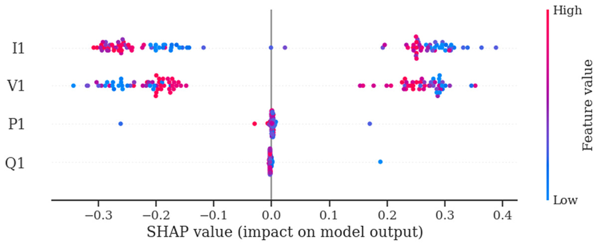
Figure 16: SHAP summary plot for the NODE model.
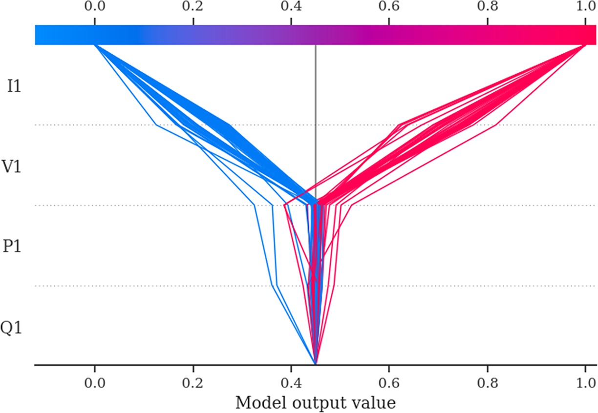
The SHAP decision plot (Fig. 17) confirms that I1 (current) and V1 (voltage) are the primary contributors of the NODE model’s predictions for voltage collapse, with consistent contributions across all samples. However, P1 (active power) and Q1 (reactive power) play again minimal roles, which indicates their limited predictive value for the NODE model.
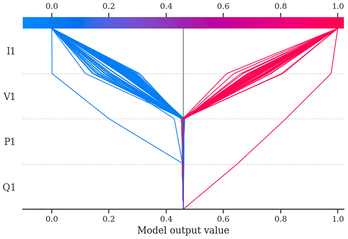
Figure 17: SHAP decision plot for the NODE model.
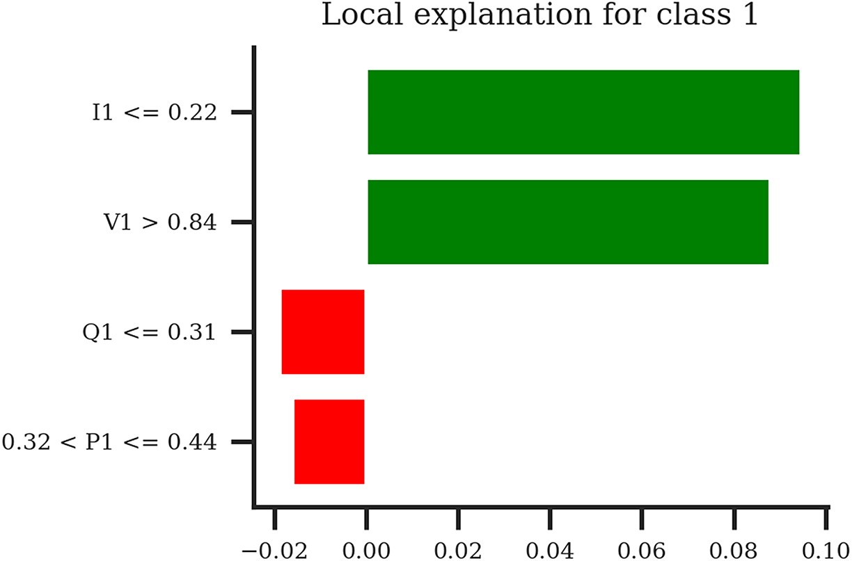
The LIME bar plot (Fig. 18) again reveals that the NODE model’s estimation for same local sample is mainly driven by I1 and V1 but unlike TabNet counterpart figure, from the low current and high voltage, which strongly support the classification into Class 1 (Voltage Collapse). The negative contributions of Q1 (low reactive power) and P1 (moderate active power) slightly counteract this prediction but are much weaker in impact.
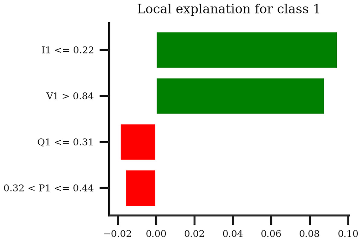
Figure 18: LIME bar plot for the NODE model for the specific sample.
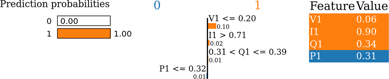
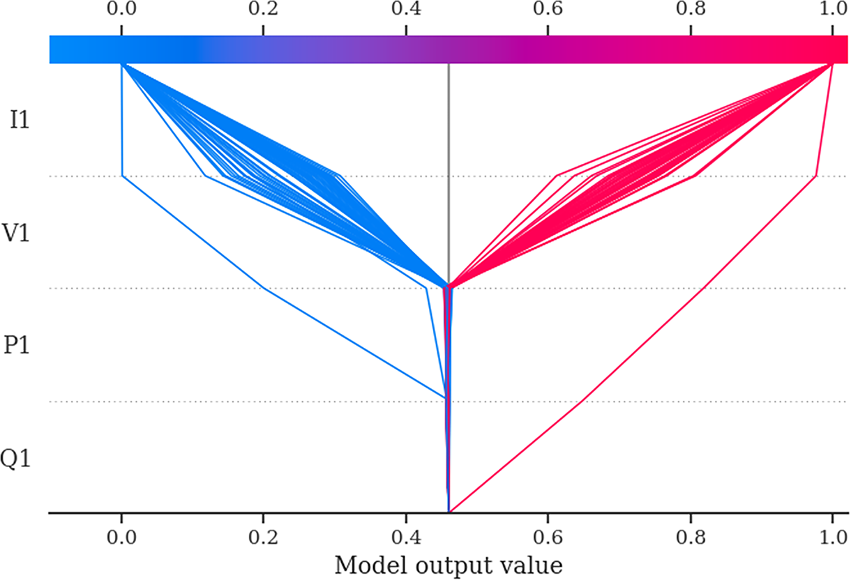
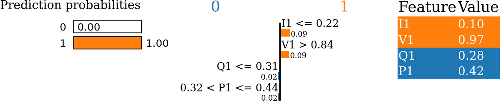
Finally, the LIME prediction plot (Fig. 19) for same particular sample shows that the NODE model’s prediction for this sample is affected this time by I1 (low current) and V1 (high voltage), both of which drive the classification into Class 1 (Voltage Collapse). Reactive power (Q1) and active power (P1) also play minor counteracting roles, with minimal impact on the estimation for this same individual sample.
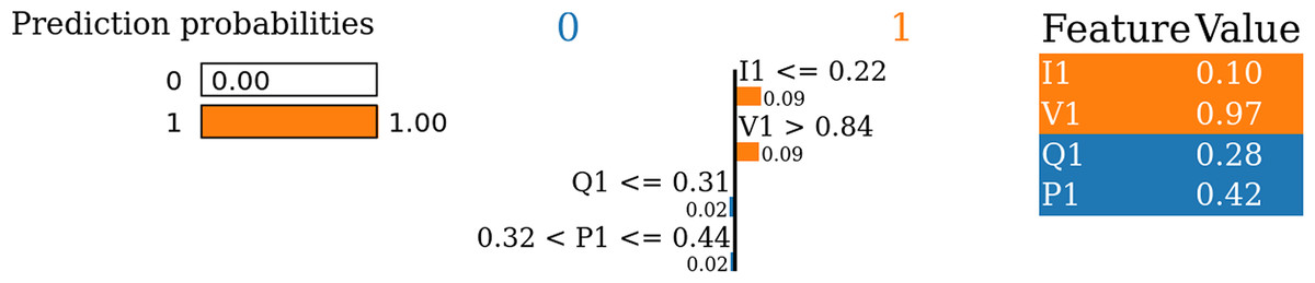
Figure 19: LIME prediction plot for the NODE model for specific sample.
An additional experiment with SHAP and LIME results
Ultimately, an additional experiment is conducted for analysis of how the TabNet and NODE models’ performance is affected in case of re-training and testing these models by using only the most influential features (I1, V1) concluded from the previous sections.
The last two-line sections in Table 3 represent the performance of TabNet and NODE models utilizing only most effective features (I1, V1). The results indicate, firstly, the TabNet model shows identical performance compared to its normal version. Secondly, the NODE model shows very slight changes in Precision, F1-Score and Accuracy with again nearly similar performance.
Consequently, this experiment shows that not only TabNet and NODE models show nearly identical performance compared to their normal counterpart models with utilizing the subset of features (I1, V1) having most influence over the decision process of these models but also the models’ complexity and computational burden are reduced thanks to using fewer features. This observation further confirms that SHAP and LIME techniques enable to identify effective feature subset and utilize these feature subset for leveraging both for preserving model performance without compromising vital accuracy decrease and reduction of the complexity and computation burden for the models.
Discussion
This study comprehensively and detailedly evaluated the performance and interpretability of TabNet and NODE models for predicting voltage collapse in the Arc Furnace dataset. The quantitative results, complemented by visual explanations using SHAP and LIME, provide critical conclusions into these models’ strengths, limitations, and applicability to energy systems. The analysis highlights the importance of advanced machine learning models in managing complex systems like electric arc furnaces, where ensuring stability and reliability is required.
For the quantitative results, we can conclude that both TabNet and NODE demonstrate notable performance by achieving an accuracy of 95% and balanced F1-scores of 0.95 for both classes. These metrics underscore both TabNet and NODE models6 ability to handle the complex, non-linear relationships in the dataset, particularly between critical features like I1 (current) and V1 (voltage) and the target variable (Collapse). SHAP analyses consistently identified these two features as the most influential predictors, reinforcing the models’ alignment with domain knowledge. LIME further illustrated how specific feature values (e.g., low current or high voltage) influenced individual predictions by providing localized explanations that increase trust in the models6 decision-making processes.
The quantitative and visual XAI (SHAP and LIME) based results further support that the importance of TabNet and NODE models for energy systems is particularly evident in this context. Electric arc furnaces are highly dynamic systems where voltage instability can bring about operational disruptions, equipment damage and financial losses. TabNet’s sequential attention mechanism and NODE’s differentiable decision trees are particularly designed at identifying subtle patterns in high-dimensional data, which makes them highly effective for real-time monitoring and fault prediction in such systems. Additionally, their interpretability, obtained through built-in attention mechanisms and compatibility with explainable AI techniques, ensures that their predictions can be understood and validated by domain experts, which is another critical requirement for applications in energy systems.
However, despite their strengths, both TabNet and NODE have certain limitations. While they outperform traditional models such as Random Forest, XGBoost, and SVM in terms of accuracy and balanced performance, their computational complexity is higher, which makes them more resourceful and computationally intensive to train and deploy. This can be a particular limitation for real-time applications or scenarios with limited computational resources. Additionally, we can also conclude both models heavily depend on the quality and quantity of input data. The performance of TabNet and NODE could degrade in the presence of noisy, incomplete, or biased data, which indicates the importance of robust data preprocessing and quality control.
This study makes several important contributions to literature. Firstly, it presents the effectiveness of TabNet and NODE models in addressing a critical challenge in energy systems, particularly for voltage collapse prediction in electric arc furnaces. By achieving state-of-the-art performance by TabNet and NODE models on the Arc Furnace dataset, this study sets a benchmark for future research in this area. Secondly, the integration of SHAP and LIME for model interpretation provides a further comprehensive framework for evaluating and understanding complex machine learning models, which potentially bridges the gap between predictive accuracy and interpretability. Finally, the study emphasizes the role of feature importance analyses in aligning machine learning insights with domain knowledge, increasing the practical applicability of the models.
Conclusions
This study comprehensively analyzes the performance and interpretability of TabNet and NODE models for predicting voltage collapse using the Arc Furnace dataset. Both models demonstrated robust classification capabilities by achieving high accuracy and balanced performance across classes, as shown by quantitative metrics such as Precision, Recall, and F1-score metrics. The interpretability of these models are further explored using SHAP and LIME techniques by providing detailed insights into the contributions of input features (I1, V1, P1, and Q1) to their estimations.
The quantitative results emphasize the effective predictive power of both models, with TabNet and NODE achieving similarly high levels of accuracy (95%). Additionally, SHAP analyses consistently indicate I1 (current) and V1 (voltage) as the dominant features for driving model predictions, while P1 (active power) and Q1 (reactive power) features contribution is minimal. This finding aligns with domain knowledge, as current and voltage fluctuations are potential indicators of voltage collapse. The decision plots further reinforced these conclusions by demonstrating the cumulative contributions of I1 and V1 to model outputs, indicating their critical role in shaping predictions. Both models effectively captured the non-linear relationships between these features and the target variable, which demonstrates their suitability for this task.
Again, the LIME analyses provide additional localized observations by showing how feature values influenced individual predictions. For specific samples, low current (I1) and either low or high voltage (V1) were the strongest predictors of collapse, with these features contributing positively to the classification into Class 1. In contrast, P1 and Q1 show minor or counteracting effects, which further supports their secondary importance. These results emphasize the models’ ability to generate interpretable and context-specific predictions, which are required for critical applications like voltage stability monitoring.
As future work, more complicated architectures such as different transformer-based networks like TabTransformer and FT-Transformer models or ensemble-based approaches are planned to run with more diverse XAI approaches additional to the LIME and SHAP methods.