
Semantic and elite moth–flame optimization algorithm-based optical-flow tracking for indoor dynamic environments
- Published
- Accepted
- Received
- Academic Editor
- Paulo Jorge Coelho
- Subject Areas
- Algorithms and Analysis of Algorithms, Artificial Intelligence, Autonomous Systems, Computer Vision, Optimization Theory and Computation
- Keywords
- Simultaneous localization and mapping (SLAM), Region-based convolutional neural network (R-CNN), Cross-layer feature pyramid network (CFPN), Elite moth–flame optimization algorithm (EMFOA), Optical flow tracking, Indoor dynamic environments
- Copyright
- © 2026 R. and N.
- Licence
- This is an open access article distributed under the terms of the Creative Commons Attribution License, which permits unrestricted use, distribution, reproduction and adaptation in any medium and for any purpose provided that it is properly attributed. For attribution, the original author(s), title, publication source (PeerJ Computer Science) and either DOI or URL of the article must be cited.
- Cite this article
- 2026. Semantic and elite moth–flame optimization algorithm-based optical-flow tracking for indoor dynamic environments. PeerJ Computer Science 12:e3498 https://doi.org/10.7717/peerj-cs.3498
Abstract
Background
Mobile robot applications rely heavily on simultaneous localization and mapping (SLAM); however, visual SLAM systems often struggle to maintain accuracy and resilience in dynamic environments. A key challenge is the ineffective filtering of dynamic feature points, which leads to localization errors. Recent advancements have introduced optical-flow techniques to remove moving objects, but further improvements are needed to enhance both accuracy and efficiency.
Methods
This research improves dynamic object filtering by introducing a region-based convolutional neural network (R-CNN) to eliminate highly dynamic objects. A cross-layer feature pyramid network (CFPN) is integrated to enhance feature extraction in dynamic scenarios. Additionally, the elite moth–flame optimization algorithm (EMFOA) is employed alongside optical-flow tracking to refine feature-point matching. The approach optimizes a classical optical flow objective across discrete grids, explicitly targeting error criteria to improve flow field quality. By leveraging the structured mapping space, computational complexity is reduced from quadratic to linear.
Results
Compared to existing methods, the proposed technique demonstrated superior precision. On the Sitting_XYZ dataset, it achieved the lowest absolute pose error (APE): mean = 0.2211, median = 0.2359, RMSE = 0.2159, and standard deviation = 0.0716. On the Sitting dataset, the classifier reduced APE mean values by 39.90%, 33.96%, 29.92%, 24.44%, 16.60%, and 8.56% compared to DGS-SLAM, YOLO-SLAM, ORB-SLAM2, OPF-SLAM, DynaTM-SLAM, and DI-SLAM, respectively. These results underscore the enhanced localization precision and robustness of the proposed system in continuously evolving environments.
Introduction
Autonomous systems encounter a fundamental challenge in accurately determining their position while traversing their surroundings. In addressing this challenge, the simultaneous localization and mapping (SLAM) issue has been the subject of much study by robotics researchers. To address this difficulty during navigation, systems must simultaneously infer a map of their environment and their relative positions (Cadena et al., 2016). Interest in SLAM technology is growing as a result of developments in drones, virtual reality, autonomous driving, and mobile robotics. There are two types of SLAM technology: there are two types of SLAM systems: lasers and visuals, that depend on the sensors employed. The emphasis of research has switched to vision-based SLAM systems because of advancements in deep learning, computer vision, and hardware computing capabilities. Drones, mobile robots, and autonomous driving are only a few of the sectors that are using this technology more and more (Chen et al., 2022).
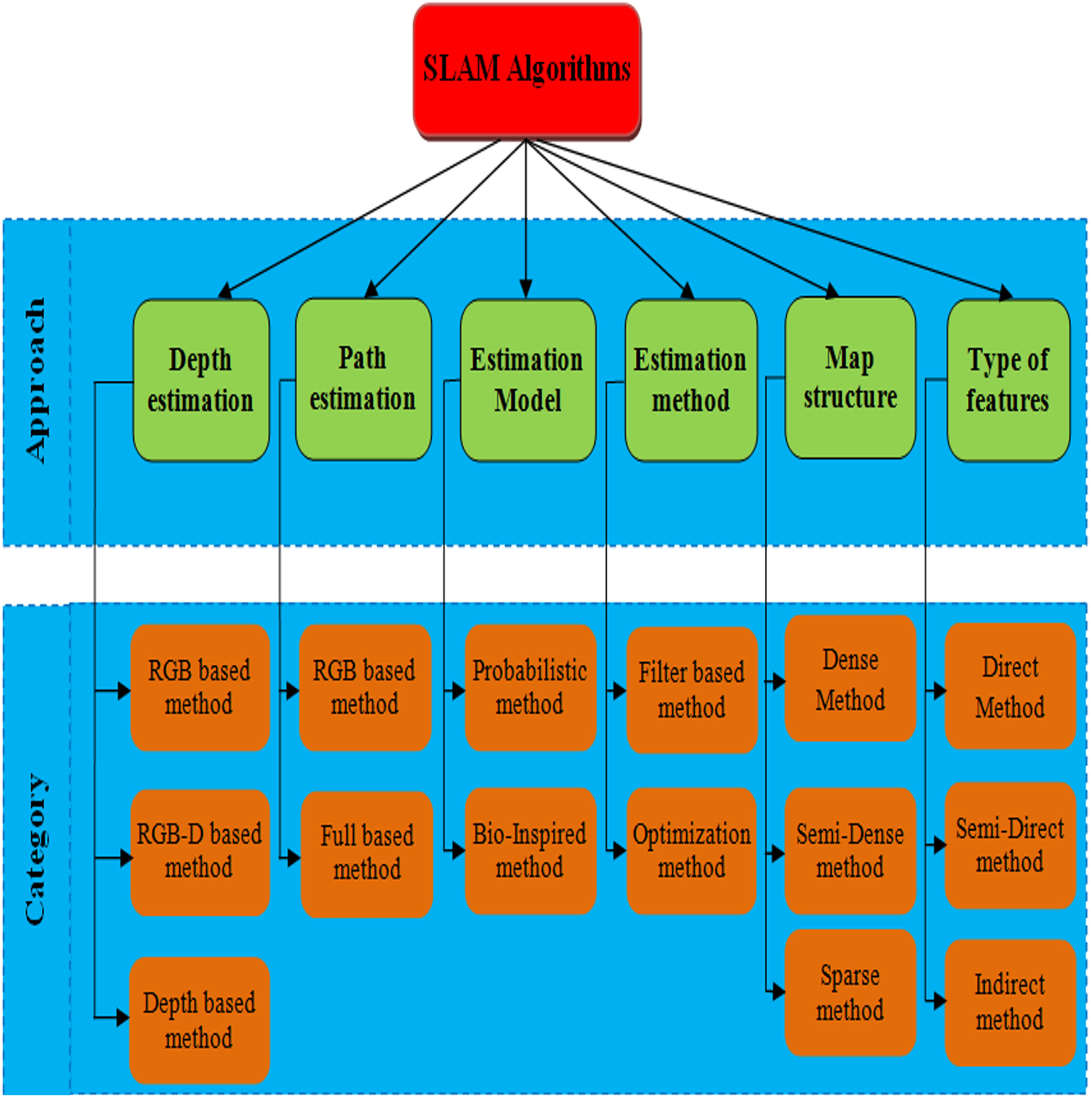
The small size, affordability, and ease of sensor assembly make visual-based SLAM algorithms particularly appealing. Consequently, the literature presents numerous visual-based techniques, ensuring the process of selecting the best one given the constraints of the project. RGB-D SLAM, Visual-only SLAM, and Visual-Inertial (VI) SLAM are the three main categories into which these methods are divided. Visual-only SLAM is more technically challenging since it only uses 2D pictures from a monocular or stereo camera. This is because there is less visual input available (Taketomi, Uchiyama & Ikeda, 2017). An inertial measurement unit (IMU), which is small and affordable and ensures high accuracy necessary condition for applications requiring a lightweight design, like autonomous race cars can be added to improve the sensor tracking robustness of visual-SLAM algorithms (Kabzan et al., 2020). Moreover, depth sensors may be integrated into visual-based SLAM systems, which then use an RGB-D-based method to interpret depth data. The major classification of SLAM based methods are shown in the Fig. 1. This work follows the procedure of depth information-based SLAM based methods.
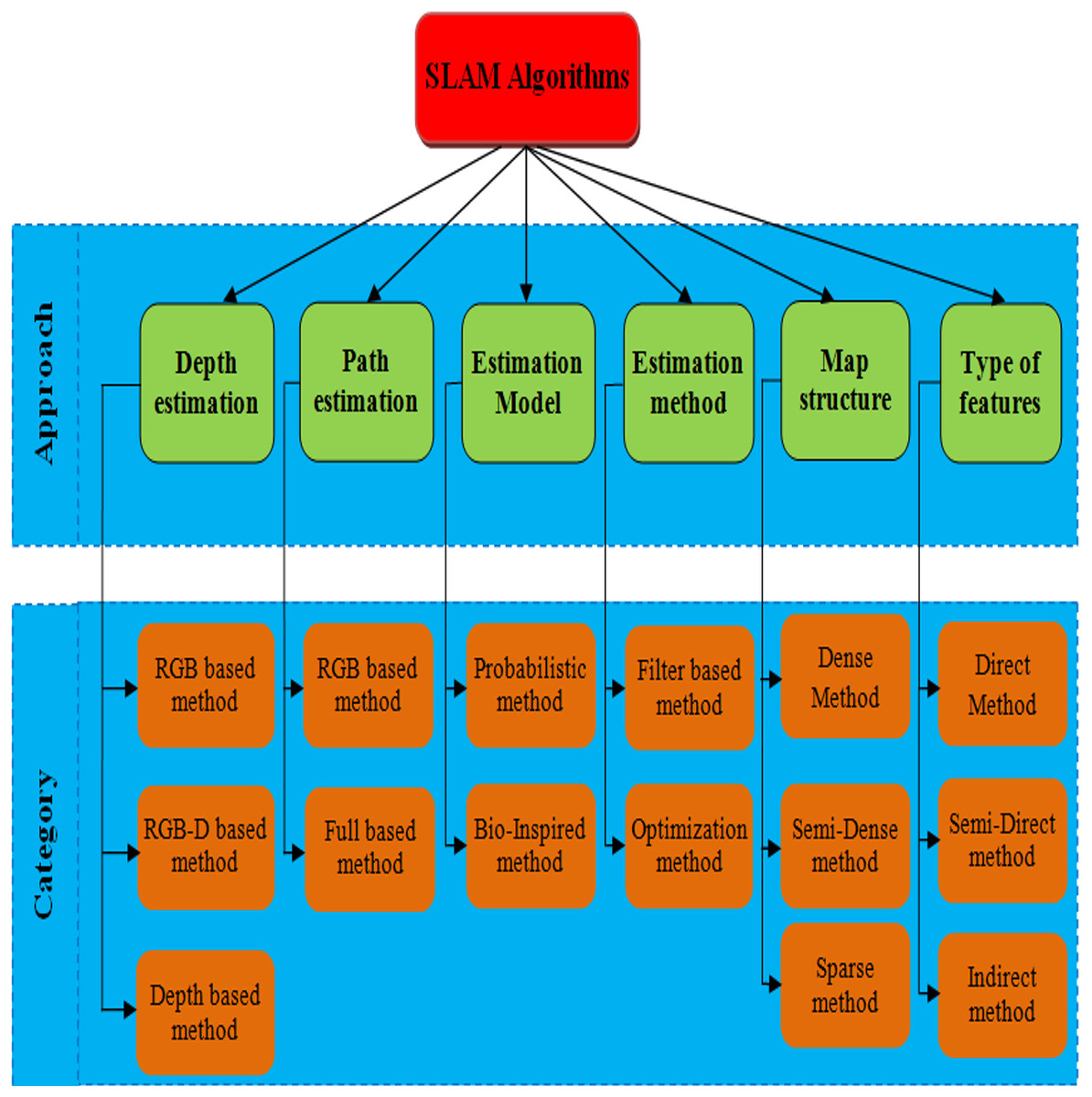
Figure 1: SLAM algorithms’ categories based on different methods (Eyvazpour, Shoaran & Karimian, 2023).
Static environments underpin visual SLAM systems. Thus, this static-environment concept supports most visual SLAM systems. While these systems perform well in static environments, the accuracy of their positioning can be significantly compromised in dynamic items, which might cause serious deviations and even system failure (Wang et al., 2019). However, real-world SLAM scenarios often deviate from the static environment assumption, featuring numerous moving objects. Due to a shortage of static features, typical vision-based SLAM systems are less successful in this dynamic environment since they have difficulty extracting steady stationary feature points (Liu & Zhou, 2022). Using several sensors and combining the data they gather to lessen the effect of moving objects on SLAM systems is one workable solution to this problem. However, integrating multiple sensors comes at a substantial computational expense (Liu, Guo & Zhang, 2022).
Numerous effective semantic-segmentation algorithms, including SegNet (Pei et al., 2021), DeepLab (Sun et al., 2022), and Mask R-CNN (Hu et al., 2022), have been proposed. These algorithms enable pixel-level classification in images, providing information about object boundaries and semantics. Despite their capabilities, these semantic methods cannot distinguish between currently moving or stationary dynamic objects, limiting their ability to precisely identify dynamic elements. Some objects, are usually moving, such as people, vehicles, and animals, and taking them out does not lead to adverse consequences (Qian et al., 2021). However, if all dynamic objects are considered in motion and removed from texture-limited scenarios like parking lots, the algorithm may lose reference points and position inaccurately. When parked vehicles (or other potentially dynamic objects at rest) are identified as transient references, positioning accuracy may be improved in locations with little roughness. Using temporary reference objects successfully requires identifying the mobility state of Possible adaptive components (Zhang, Zhang & Wang, 2022). The Optical-flow approach is added to images to overcome the difficulties faced by systems for SLAM in constantly evolving settings.
Zhong et al. (2018) presented a new robotic vision system has been developed, integrating SLAM to establish a beneficial link between the two functions using a deep neural network-based object detection. This innovative system enables a robot to efficiently and reliably perform tasks in unfamiliar and dynamic environments. It does not follow any descriptor for object detection. It has been solved by DynaSLAM. Bescos et al. (2018) introduced FAST and Rotated BRIEF-Simultaneous Localization and Mapping 2 (ORB-SLAM2) were enhanced by the introduction of DynaSLAM, a visual SLAM system. DynaSLAM employs various techniques, for detecting moving objects, such as multitier geometry and deep learning. For long-term applications in real-world settings, DynaSLAM accurately predicts a map of the scene’s static features and performs typical visual SLAM baselines in extremely dynamic conditions. Bounding boxes presented in the dynamic environments has not been focused by ORB-SLAM2. It has been focused by R-CNN.
He et al. (2017) presented introducing a straightforward, adaptable, and flexible object instance segmentation framework, this technique accurately creates segmentation masks for each instance of an object while simultaneously detecting objects in an image. A parallel branch devoted to object mask prediction is included for a boundary to the current branch identification in this method, which is called Mask R-CNN, which builds upon Faster R-CNN. It even outperforms the Common Objects in Context (COCO) 2016 challenge winner. It does not focus on the semantic segmentation of objects, thus it has been focused by visual SLAM.
Yu et al. (2018) introduced an effective and reliable system for providing relevant visual assistance in dynamic settings (DS-SLAM). DS-SLAM concurrently operates on five threads: track, segment, map, close, and generate dense semantic maps. To improve localization accuracy in dynamic circumstances, DS-SLAM employs a dynamic consistency check approach and a semantic segmentation network to more efficiently lessen the influence of approaching products. Experiments show impressive performance in real-world conditions and on the TUM RGB-D dataset. DS-SLAM to ORB-SLAM2, the absolute trajectory accuracy obtained shows an order of magnitude increase.
Cui & Ma (2019) initially presented this visual semantic SLAM system, the RGB-D mode of ORB-SLAM2 provides the basis for Semantic Optical Flow SLAM (SOF-SLAM). It is made specially to deal with changing situations. Semantic optical flow is a novel method for dynamic feature detection that is suggested. SegNet produces a dependable basic matrix by using the pixel-wise in the semantic optical flow, semantics segmentation produces masks. In dynamic situations, our method guarantees precise camera pose estimates. Real-world situations and the TUM RGB-D the dataset is used for experimental investigations. Precision system SLAM is still reduced due to sparse problem; it has been enhanced by the Delaunay triangulation.
Dai et al. (2020) proposed SLAM technique, moving objects in dynamic situations are intended to have less of an influence. The method leverages the correlation among map points to differentiate points connected with different moving objects from those that belong to the static scene, segregating them into separate groups. Initially, all map points are used to create a sparse graph by Delaunay triangulation. SLAM methods have been extended to deep-learning-based methods. To identify and segment objects and eliminate outliers, it primarily focuses on both geometric and semantic information. In addition, object detection has been also enhanced by introducing YOLO method.
Fan et al. (2022) presented a BlitzNet in indoor dynamic situations with a semantic SLAM system (Blitz-SLAM). In combining data from masking that is geometric and semantic in nature, the local point cloud’s noise blocks are effectively eliminated using Blitz-SLAM using RGB and depth images. By combining many local point clouds, a global point cloud map is produced. Blitz-SLAM is evaluated using real-world settings and RGB-D the TUM dataset’s data. On the basis of the experiment’s results, Blitz-SLAM generates an accurate and thorough global point cloud map and is effectively in dynamic scenarios.
Yang et al. (2020) introduced as Semantic and Geometric Constraints Visual Simultaneous Localization and Mapping (SGC-VSLAM), modules for static point cloud map generation and dynamic detection are included in this system, ORB-SLAM2’s RGB-D mode is used in the construction. To improve the ORB-SLAM feature extractor’s performance, SGC-VSLAM employs an improved quadtree-based technique. To determine a more accurate basic matrix across subsequent frames, it makes advantage of You Only Looks Once, version 3 (YOLO v3) is responsible for producing the semantic bounding box seen above. Studies to evaluate the proposed technique utilize the TUM RGB-D dataset. Semantic information has a major role with object identification methods based on deep learning, segmentation, and outlier removal.
Yan et al. (2022) suggested a Dynamic RGBD SLAM approach, termed DGS-SLAM, which integrates both geometric and semantic information. Firstly, the technique uses the multinomial residual model to develop a new module for the identification of dynamic objects. Movement data collected by the semantic segmentation modules is used by this module to segment motion. along with motion residual information from neighbouring frames. Second, feature point classification results are used to construct a camera pose-tracking method for reliable system tracking. Lastly, using the results of camera tracking and dynamic segmentation, a semantic frame selection approach is developed to produce a semantic segmentation module that extracts potentially moving items in the image. Comprehensive tests using public datasets from TUM and Bonn demonstrate that DGS-SLAM is effective performs faster and more robustly in dynamic settings than modern dynamic RGB-D SLAM systems.
Wu et al. (2022) presented a dynamic-environment-robust visual You Only Look Once with SLAM (YOLO-SLAM). The design incorporates Darknet19-YOLOv3, accelerating and producing essential semantic data for the low-latency backbone of the SLAM system. Unique geometric constraint technique is presented to identify dynamic characteristics inside detecting regions. Random Sample Consensus (RANSAC) is utilized to recognize these dynamics characteristics by taking advantage of depth differences. Experiments on challenging dynamic sequences from the purpose of the TUM and Bonn datasets is to evaluate the efficacy of YOLO-SLAM.
Chen et al. (2022) presented, a unique monocular SLAM algorithm created for dynamic situations. Initially, an adapted Mask R-CNN is employed to eliminate previously identified highly dynamic objects. Subsequently, a basic matrix is determined based on the matched pairs use the optical-flow technique to match the remaining feature points. The suggested technique greatly improves the accuracy of posture estimate in a SLAM system, based on experimental findings utilizing the RGB-D dynamic datasets from Bonn and TUM, particularly in high-indoor dynamics circumstances.
Zhong et al. (2024) suggested a reliable semantic visual a dynamic SLAM system setting referred to DynaTM-SLAM. Dynamic objects’ impact is considerably limited by rapidly and effectively filtering out the true dynamic feature points using a sliding window when used with DynaTM-SLAM, object identification, and template matching algorithms. The DynaTM-SLAM technique detects dynamic items using object detection rather than the laborious semantic segmentation. Furthermore, on the internet, an object database is being developed, and by applying semantic restrictions to the static objects, optimized camera, map, and object positioning. This method assists to increase the precision of ego-motion estimate in dynamic situations and completely utilizes the beneficial influence of static objects’ semantic information. Performance in dynamic situations has significantly improved, according to experiments conducted on the TUM RGBD dataset.
Yao, Ding & Lan (2023) introduced MOR-SLAM, a mask repair technique that can provide precise system monitoring and dynamic positioning interior situations and identify dynamic objects with accuracy. The ORB-SLAM2 is enhanced with an instance segmentation module to generate a preliminary mask and differentiate environment’s dynamic and static elements. The accuracy of object masks is then guaranteed by a new mask inpainting model that fixes both tiny and big items in the image using the morphological and depth value fusion methods, accordingly. On the basis of the previously corrected mask, a trustworthy fundamental matrix may then be produced. The static feature points are sent into the system’s tracking module via the reliable basic matrix after likely dynamic feature points in the environment have been identified and eliminated utilizing high-precision positioning and tracking in dynamic situations.
Wei, Xia & Han (2025) expanded the possibilities of ORB-SLAM3 to create DI-SLAM, an improved SLAM method for dynamic interior situations in real time. YOLOV5S, a DI-SLAM technique, filters dynamic characteristics for initial monitoring and is bound semantic data from every input frames. To increase the precision and resilience of localization systems, multi-view geometry is also used to better distinguish changing feature information. Additionally, to prove the technique worked, TUM RGB-D dataset tests were done.
Cong et al. (2024) suggested the YOLOv5 deep-learning technique and the dynamic visual SLAM (SEG-SLAM) system using the oriented FAST and rotated BRIEF (ORB)-SLAM3 architecture as the basis. First, the ORB-SLAM3-based YOLOv5 deep-learning technique is used to build a target recognition and semantic segmentation fusion module. From possibly changing objects, this module has the ability to rapidly find and retrieve earlier data. Secondly, novel dynamic features point rejecting methods are developed for dynamic objects based on previous experience, depth information, and epipolar geometry. SEG-SLAM’s mapping and localization precision improves. Fusing the disregarded results with depth data produces use the Point Cloud Library to create a static, dense 3D map devoid of dynamic elements. SEG-SLAM is tested using real-world scenarios and public TUM datasets. The recommended technique outperforms dynamic visual SLAM systems in accuracy and reliability.
Huai et al. (2025) motions blur’s effect on visual SLAM systems by using a unique visual SLAM algorithm that integrates many ways to provide more dependable semantic information. In particular, the SLAM system is enhanced with a missing segmentation compensation method to forecast and restore semantic information, which is then used for generating masks of dynamic objects. This allows for the precise separation of moving items from static ones. To improve keypoint filtering, the SLAM system also incorporates dynamic feature identification and exclusion using probability. In dynamic interior situations with large view angle fluctuations, the SLAM system achieves lower absolute trajectory error (ATE) than previous approaches using the RGB-D datasets from Bonn and TUM. This method can increase domestic robots’ autonomous navigation and scene understanding.
However, a difficult research topic is how to combine object recognition with the SLAM algorithm to ascertain an item’s motion status in real-time situations. The SLAM system’s accuracy may be greatly increased by removing efficient use of static object data and dynamic feature points. The majority of SLAM algorithms that concentrate on dynamic scenes, however, are mostly focused on removing dynamic items to maximize efficiency, and therefore fall short of fully using the potential advantages of static objects’ semantic information. Many SLAM systems, however, disregard the issue that the segmentation network’s image mask cannot delete point features and represent movement objects. As a result, even after the dynamic objects are eliminated, the environment will still absorb some dynamic feature points., influencing the estimated camera position inaccuracy.
These issues has been solved by introducing Optical-flow tracking. Optical flow-based methods are sensitive to even the smallest motion and operate in real-time, allowing them to precisely detect and identify the location and there is no need for scene information to determine the motion state of moving items. Optical flow-based approaches, on the other hand, struggle with degenerative motion, are prone to lighting effects, and operate on the premise of constant brightness. Elite Moth–Flame Optimization Algorithm (EMFOA), whole set of mappings between discrete grids are optimized and updated in the optical flow tracking. Optical flow tracking often deals with noisy or unpredictable motion. EMFOA adaptive search helps avoid premature convergence and local optima. A number of iterations were performed to monitor the pixels in the optical flow tracking, EMFOA produced the solution with the most significant result. The following describes the work’s main contribution,
In this work, to improve dynamic visual SLAM system reliability, monocular dynamic visual SLAM was created.
An enhanced version of Mask R-CNN has been developed to achieve more precise segmentation of previously challenging extremely moving items in dynamic interior settings. This improvement aims to fulfil the specific demands of SLAM algorithms operating in dynamic scenes.
Optical-flow tracking is introduced to exclude very dynamic elements from dynamic situations. Elite Moth–Flame Optimization Algorithm (EMFOA), whole set of mappings between discrete grids are optimized and updated in the optical flow tracking.
The suggested system outperformed the present approaches in terms of performance.
Proposed methodology
In this article, adjusted Mask R-CNN has been introduced for removing prior highly dynamic objects. A module and branch specifically tailored for dynamic environments known as the CFPN have been incorporated. The remaining pairs of feature points are matched through the Elite Moth–Flame Optimization Algorithm (EMFOA) to Optical-flow Tracking, leading to the calculation of a fundamental matrix using these matched pairs. The approach optimizes a standard optical flow objective over all possible mappings between discrete grids. This optimization process directly enhances the error criterion used to assess the flow field’s quality, eliminating the need for approximations like maximum-likelihood estimation for such problems. Tens of thousands of nodes can be efficiently matched to tens of thousands of displacements according to improvements that lower the inner loop of the algorithm’s computational cost from quadratic to linear and to the mapping space’s highly ordered structure. The performance of the suggested system exceeded that of the current approaches.
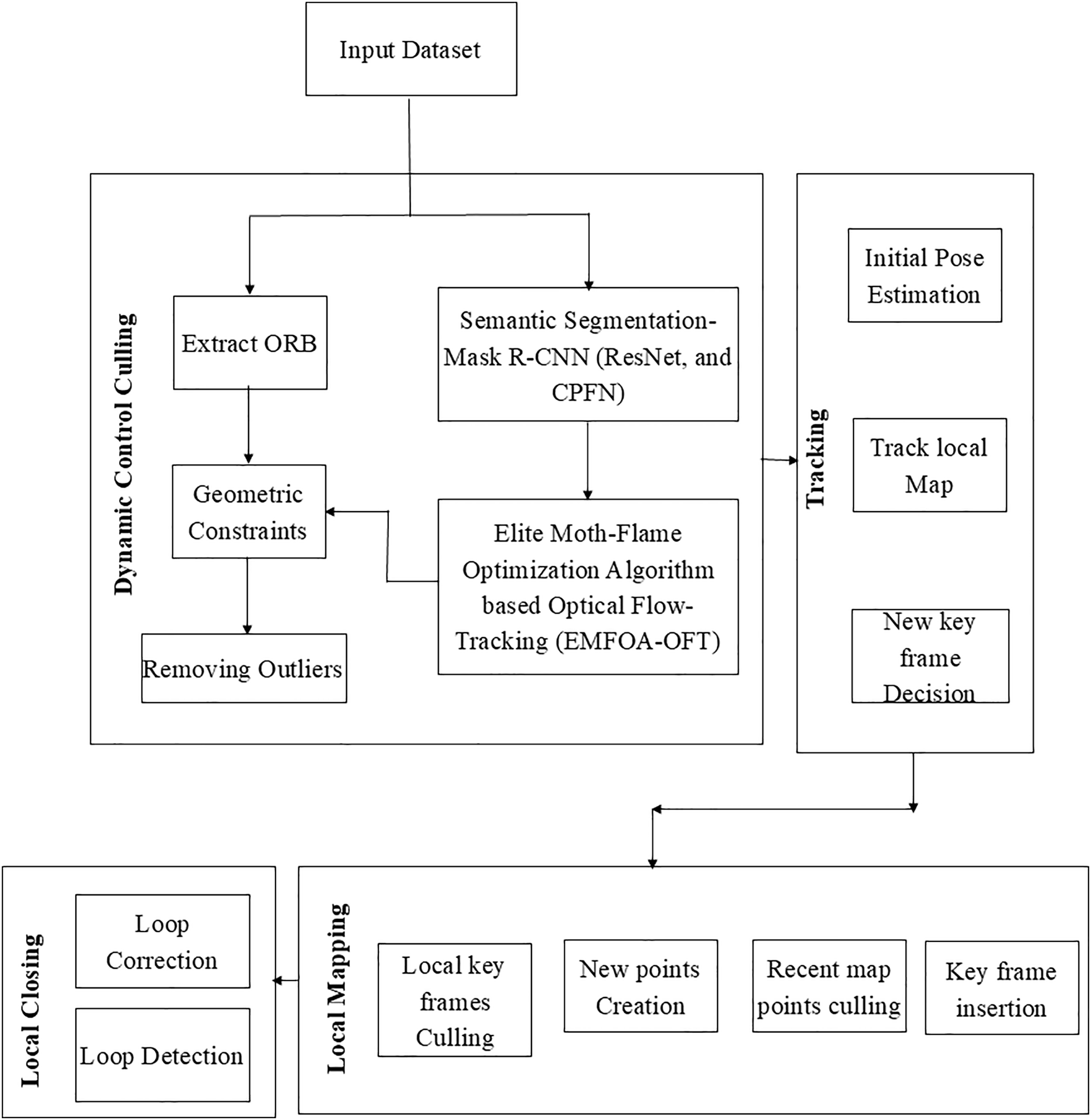
The proposed dynamic SLAM algorithm incorporates an additional thread dedicated to handling moving objects, introduced alongside the existing threads for actual tracking, local construction, and loop detection. Figure 2 illustrates the modified system framework. The threads used for loop detection and local map creation are still the same as in ORB-SLAM2. The former records the environment, whereas Bundle Adjustment (BA) optimizes camera attitude.
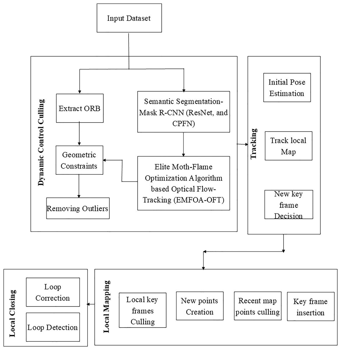
Figure 2: Proposed vlsam framework.
Dynamic content culling
The method of handling dynamic objects consisted of three consecutive phases: semantic segmentation, dynamic feature removal and optical-flow feature tracking. The procedure unfolded as follows: (1) The segmentation network was given RGB images, the system utilizes ORB feature extraction from RGB images to detect and eliminate feature points of previously highly dynamic objects; (2) following that, there was a motion continuity check that included three steps: determining an extraction of dynamic feature points, extracting dynamic points using polar constraint, and determining the basic matrix between two successive frames and optical-flow tracking; (3) The dynamic feature removal module utilized these positions to assess whether image objects were moving following the motion continuity check. In such case, the moving object’s ORB feature points were removed. Subsequently, to enhance tracking and map construction, the SLAM system included the remaining static feature points.
Semantic segmentation
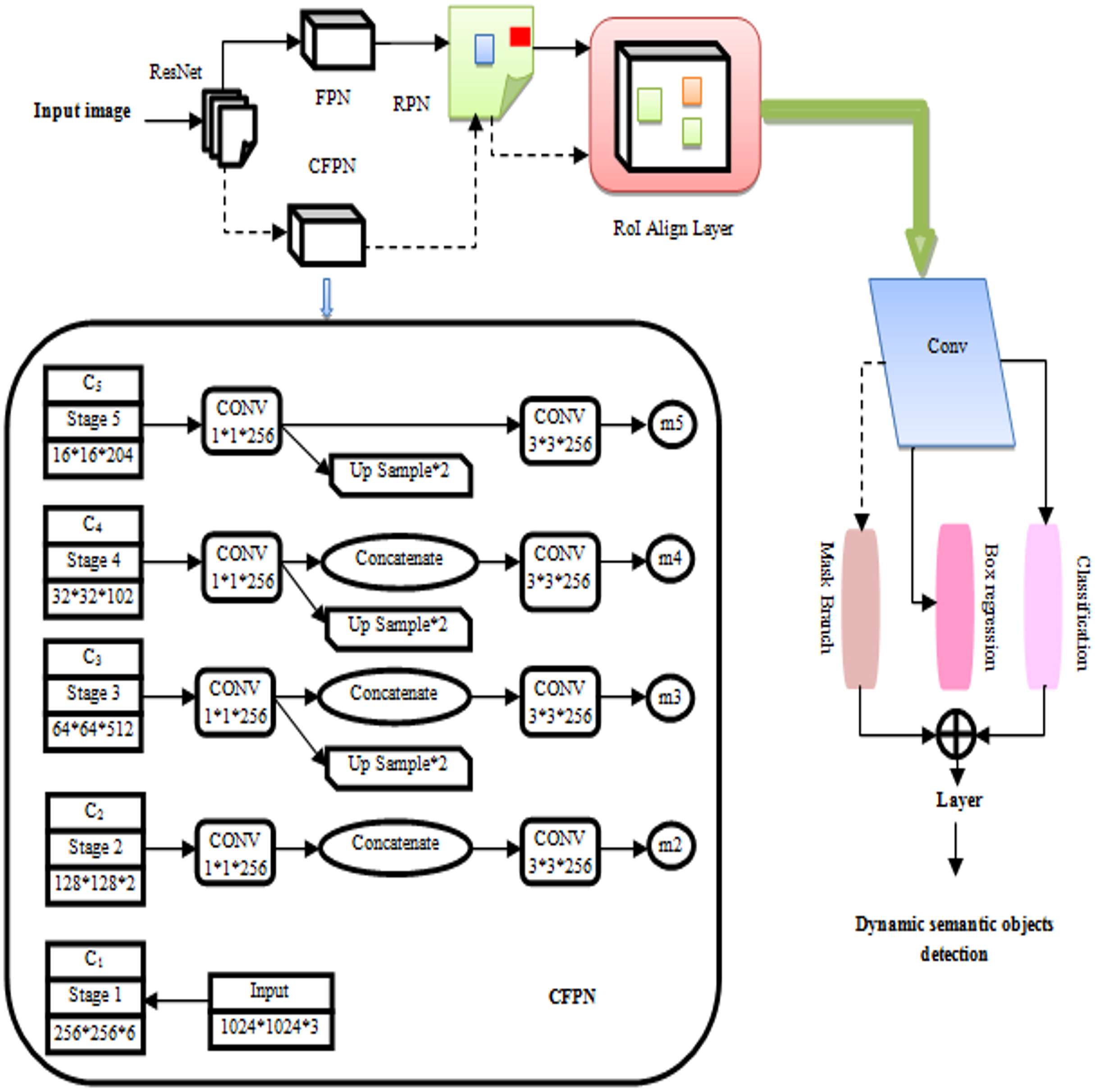
Dynamic images show improved semantic segmentation with mask R-CNN. Mask R-CNN features are extracted by ResNet and organized into use a Feature Pyramid Network (FPN) as a backbone network. Figure 3 shows the fine-tuning procedure that the Mask R-CNN undertook. Figure 3 shows the procedure by which the Mask R-CNN was refined in this investigation. For dynamic situations, a branch and module for a cross-layer feature pyramid network (CFPN) were developed. By reconstructing backbone network for feature extraction, the objective was to make more use of contextually semantic data. In contrast to candidate boxes were generated by the region proposal network (RPN) and the original network, the FPN-processed feature group. The Mask R-CNN branch for segmented tasks only received CFPN-fused feature group and candidate boxes after RoI Align, while it was only employed for regression and categorization after the RoI Align procedure (Zhang, Wang & Zhu, 2021). RoI Align was performed, before the Mask R-CNN segmentation of all the candidate boxes and the CFPN-fused feature group. The Mask R-CNN branches now include an enhanced CFPN module when it was realized that adding multi-dimensional features directly would not be advantageous for later full-convolution segmentation tasks. With this improvement, semantic information from many levels may be used more comprehensively, which improves network performance when segmenting previously highly dynamic items within an environment.
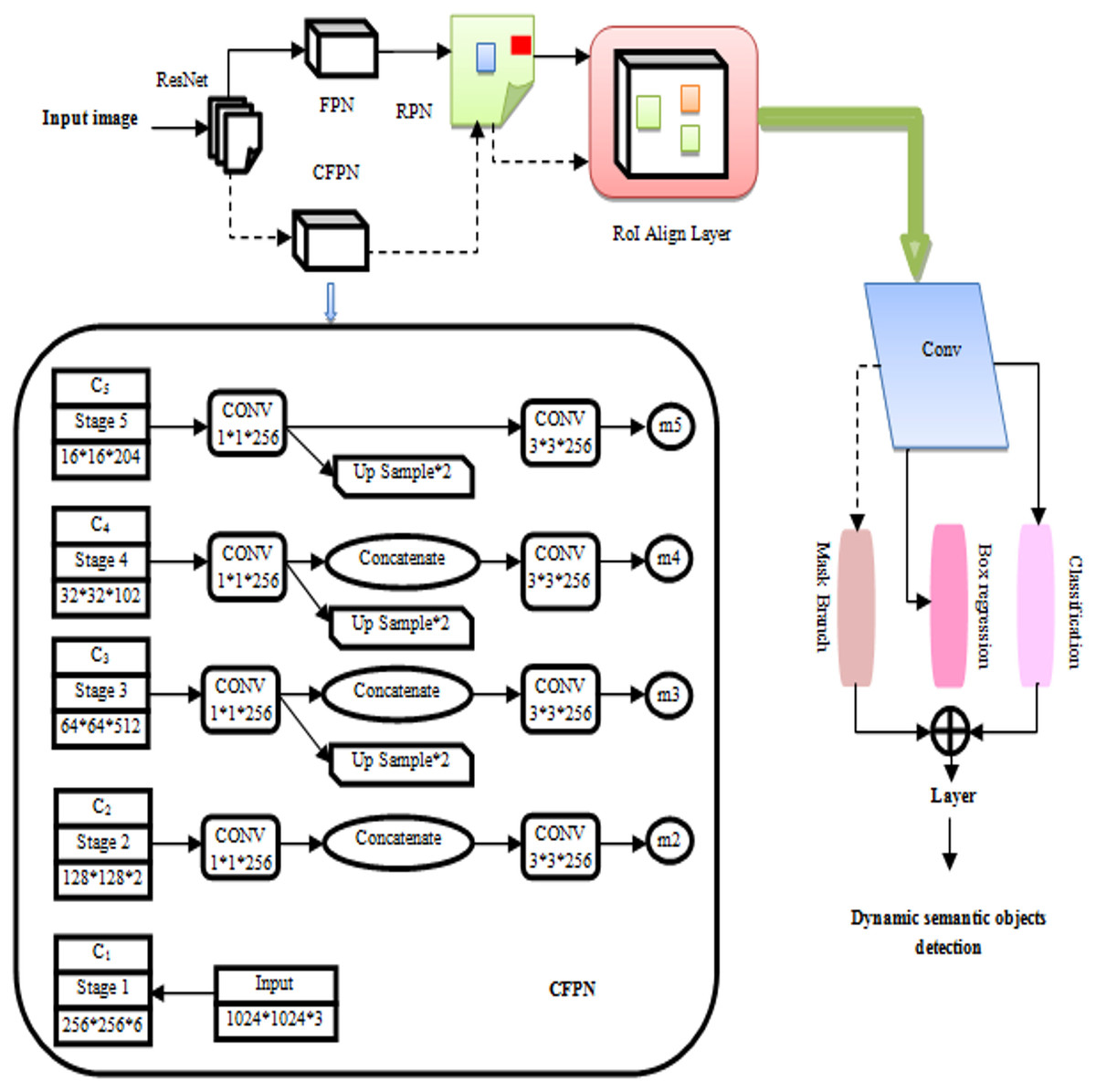
Figure 3: Improved mask R-CNN algorithm.
To maintain the size of the feature map while simultaneously reducing dimensions, each layer’s properties were convolved using a “1 × 1” convolution kernel. ResNet’s recovered features were designated C1–C5. Upsampling was used to add features from the bottom layer and twice after the C3–C5 convolutions, the feature map’s size. To accomplish dimensionality reduction and remove the aliasing effect after upsampling, a “3 × 3” kernel was utilized for convolution on each fused feature. Using convolution and direct upsampling of C5, “m5” was created, high-level features were upsampled and low-level features merged to generate “m2” to “m4”. Mask R-CNN branches were applied to the m2, m3, m4, and m5 feature groupings. CFPN upsampled retrieved stage features and mixed them with low-level characteristics to generate m2, m3, m4, and m5. CFPN and the candidate box performed Mask R-CNN branch ROI Align.
Optical-flow tracking by elite moth–flame optimization algorithm
The remaining feature pairs were aligned using optical-flow tracking points after the first highly dynamic items were eliminated by fine-tuning Mask R-CNN. Next, they used the matched feature-point pairs to compute a simple matrix. The use of a polar geometric restriction ultimately assisted to further improve the environmental dynamic feature points. The optical-flow technique is widely employed for motion detection (Zhou & Zhang, 2022), encompassing partial pixel motion calculations for the entire image, commonly referred to as sparse optical flow. The basic technology used in this research is the dense daisy-descriptor framework from Daisy Filter Flow (DFF). While the original work of DFF concentrated on matching images across various scenes, the emphasis in this context is specifically directed toward addressing the challenges posed by large displacement optical flow. Estimating the flow field’s labeling for every pixel is required given a pair of images and . Markov random field formulation using a label field in a dense descriptor flow structure . Daisy descriptor scale s(p) and angle (p) for every pixel p. DAISY efficiently computes related quantities. For efficient processing, convolution is used to add the weighted contributions of each gradient vector to many description vector components.
It consists of two steps: online matching of the calculated cost, and Daisy description and image gradient pre-calculation. During the pre-computation phase of the descriptor, a collection of convolved orientation maps is denoted as is calculated for the image Im. These maps are computed for different values of and . On the other hand, for the image, a typical upright Daisy is pre-calculated . A Daisy that is resized and rotated description may then be generated based on a hypothetical on-demand candidate label l using the convolved orientation maps in the online matching step. The theoretical label is produced following the principles of the Patch MatchFilter (Yang, Lin & Lu, 2014), using random resampling and iterative neighbour propagation. For each hypothetical label, the raw matching cost is calculated considering image color, gradient, and descriptor distances. In a linear time, filter-based inference, estimating edge-preserving flow involves adaptively aggregating this raw matching cost. The method iterates over the available labels to find the one with the minimum matching cost.
The formulation of the matching cost is expressed in Eq. (1). This equation calculates the similarity of corresponding points by evaluating the distance between their Daisy descriptors. In the pixel p of image Im, (i) the standard unscaled upright description ; (ii) the scaled and oriented descriptor the translation of p′ in the pixel is image Im′.
(1) The additional terms in Eq. (1), namely the second and last terms, enhance the original descriptor distance by incorporating considerations for brightness and gradient constancy. In comparison to the original histogram-based descriptor, this improvement seeks to increase localization accuracy. A lower matching cost indicates a better likelihood that the hypothetical label is a match, as do a decreased brightness and gradient difference. The gradient constancy costs and color costs are weighted according to their respective parameters, α and β. The items that only appear in one view or the outlier caused by occlusion are the reasons for the adoption of the thresholds and . For each of the three feature terms descriptor, color, and gradient termstruncated distances are used to ensure their robustness, as stated in Eq. (1). Equation (2) involves adaptively aggregating the raw matching cost , this was determined for Eq. (1)’s pixel p and label l, over all the pixel’s q inside a window in the neighborhood of the radius r. In image , the weighting cost ( ) measures the similarity of pixel p to its neighbour q in terms of intensity and spatial proximity. Local window size increases brute force computing linearly. Regarding its filtering quality and complexity trade-off, the linear-time guided filter technique (Lu et al., 2018),
(2) Winner-Takes-All (WTA) is the simplest strategy for finding the best label as it minimizes the total matching cost in the following ways in Eq. (3),
(3) Even in the event that the filter-based inference produces favorable performance, it still takes a lot of time to thoroughly evaluate the unprocessed and combined costs and as in Eqs. (1) and (2) for every label . The reason for this is that the complexity increases with the size of the label space with high dimensions, as shown by , where represents each domain’s distinct search spaces . With a somewhat lower level of complexity, in terms of translation, rotation, and scale, EMFOA is capable of doing nearest neighbor searches domains in the O(log|L|) search range. The ORB feature points were tracked and matched using the optical-flow technique as, if the pixel’s motion velocity (u and v) were known; it was possible to estimate a single pixel’s location across several images.
Elite Moth–Flame Optimization Algorithm: Moths, classified within the arthropod phylum, are employed in the Daisy Filter Flow (DFF) process to explore the optimal label field. Typically, moths exhibit a nocturnal behavior, utilizing moonlight for navigation. Their flight pattern involves maintaining a consistent angle with the moon to ensure a straight trajectory. To achieve efficient navigation during the search for the best label field, moths employ the distance from the target (fame), activating a helical motion pattern as the distance diminishes, aligning the moth with the target (Shehab et al., 2020; Kaur, Singh & Salgotra, 2020). In the context of the DFF’s search for the best label field, each individual moth in the optimization process, represented by the EMFOA, embodies a potential optimal solution. The position of each moth is articulated as a decision matrix in Eq. (4) (Xu et al., 2019),
(4) For each i in the range . DFF label field size is n, and moths are N. The moth fitness vector is shown below Eq. (5) (Li, Zhu & Liu, 2020),
(5) The fitness is determined by how similar a pixel (p) is to its neighbour (q) in Eq. (6). Since all of the moths fly about famous, the size needs to match the moth matrix that was previously specified (Dai et al., 2020),
(6) The fitness is computed depending on the DSC. The fame matrix’s associated fitness is shown below Eq. (7),
(7) For the label field in the DFF to provide the desired results, Moth must go through the fame. Logarithmic spiral function replicates moth spiral movement, which is described by Eq. (8) (Li et al., 2022),
(8)
(9)
(10) Amoth at position is known as , which represents its distance from its associated fame ( ). To determine how near the moth and its fame are, the random values B and t range from −1 to 1, are what decide the spiral fight search in Eqs. (9) and (10). The next position of the moth and its mathematical construction are shown. In this context, represents r is a constant that ensures convergence and whose value decreases with time, k is a random integer between 0 and 1, and the maximum number of repetitions. Based to their global and local search fitness values, the fame positions from the previous and current iterations are gathered and arranged at each iteration. Only the top N.FM fames, where N.FM represents a specified number, are retained, while the others are discarded. In terms of fitness, the highest and lowest levels, accordingly, are represented by the first and last popular. Following that, moths obtain fames sequentially. The same moths or lower-order moths obtain the ultimate renown all over multiple iterations. MO and FM are represented as the moth and fame respectively. Equation (11) determines the reduced frames (N.FM) throughout iteration.
(11) From this optimal label field L of the DFF has been found using the EMFOA. To augment exploration capability, to improve exploitation, the influence of the best flame is added and a Cauchy distribution function is included. A balanced approach between exploration and exploitation is maintained through adaptive step size and iterative division. The updating mechanism for EMFOA is governed by the Eq. (12), outlined below,
(12) where the jth flame-ith moth distance is represented by the symbol . In this instance, the spiral’s form is determined by a constant, b, and t, an indeterminate integer from 1 to −1. Determining the step size of the moth’s approach to the flame that is how closely the moth’s next location matches the flame is very dependent on the parameter t. The distance between the moth and the flame is greatest when t = −1 and greatest when t = 1. The heavy-tailed character of the Cauchy distribution is the reason for using a Cauchy-based random number. Premature convergence problems are mitigated by this inclusion, which makes it easier for potential solutions to escape local minima. Equation (16), this follows the location update in each iteration and is derived from Eq. (13) specifies that the Cauchy-based random number is utilised. Notably, just the initial half of the maximum number of iterations is used to apply this technique, emphasizing the necessity for extensive exploration in the early stages.
(13)
In this context, the expression sign (rand-0.5) can assume three values: 1, 0, and −1. Combining the sign (rand-0.5) with the Cauchy leap results in an extended random walk with larger step sizes. Using the Cauchy distribution formula, which is as follows, the Cauchy operator is used to produce a random number in Eq. (14),
(14) Cauchy density function is calculated as follows Eq. (15),
(15) With is the parameter, the parameter g is set to 1. After solving Eq. (16) get,
(16) In the proposed methodology, the impact of the best-searching label L is considered for all moths. In this context, each moth adjusts its position based on both its respective flame and the best flame associated with searching label L. The moths collectively shift toward the average pixel position of the best label L, aiming to eliminate dynamic objects and their corresponding flames. This adjustment promotes exploitation by directing the moths towards the best flame, thereby enhancing convergence speed. Notably, in the second half of the iterations, when more attention on exploitation is necessary, the impact of the best flame is only included. The updated Eqs. (17), (18) are as follows:
(17)
(18) In this context, the parameter “a” function as a linearly decreasing factor, operating as a layer of protection to limit the impact of the best flame and its corresponding counterpart. After many repetitions, “a” change in value from 0.4 to 0.2. The matching flame’s impact is more noticeable in the early stages when a larger value of the “a” parameter is maintained. This emphasis makes it easier for the moths to effectively explore the search area. Later on, when the algorithm gets closer to the optimal flame, the value of “a” is reduced, which speeds up the process of convergence. To generate opposites to the current particles located in the search dimension of the best label L, Elite Opposition Based-Learning (EOBL) makes use of the elite member of the current population. This method enables the distinguished member to direct the particles, finally guiding them toward a favourable region where the optimal label may be found. Therefore, the use of the EOBL approach improves the variety of individuals in the community and strengthens the ability of the EMFOA to explore. The opposing position is expressed as follows: The elite opposite position will be , stated as Eq. (19), for the individual in the present population .
(19)
(20) where and F is a generalization factor. and are dynamic boundaries, and can be formulated as in Eq. (20). The ensuing reverse, however, could go outside the search parameters . To resolve this issue, the transferred person in , is given a random value, as in Eqs. (21), (22),
(21)
| INPUT: is the function that is being evaluated. Other relevant parameters have been determined, like the population’s number of mathematics (N), dimension (d), maximum iteration (Maximum_iter), flame number (N, FM), b, and others. |
| OUTPUT: With the least amount of fitness function, the best label L solution |
| For i = 1: N |
| For j = 1:d |
| Use Eq. (22) to generate N organisms (i = 1…N), |
| (22) |
| End for |
| End for |
| Calculate fitness |
| While Current_iter<Maximum_iter+1 |
| If iteration==1 |
| Enter the starting population, N, FM = N |
| Else |
| Employ by Eq. (11) |
| End if |
| FM=fitness function f(X) |
| If iteration==1 |
| Create the moths in accordance with FM |
| Update |
| Iteration = 0 |
| End if |
| Arrange the moths according to FM from |
| Update and Elite Opposition Based-Learning (EOBL) |
| End if |
| For j=1:N |
| For k=1:d |
| Find the r and t using Eqs. (9), (10) |
| Using Eq. (18), make updates to the moths’ position based on their particular flame |
| End for |
| End for |
| Current_iter=Current_iter+1 |
| End while |
Optical-flow tracking proves effective in preventing erroneous matches. The process involves multiple iterations to iteratively track pixels, aiming to achieve the most effective solution. The fundamental matrix F for these point pairings is constructed when corresponding matching points have been obtained. The remaining essential the image’s filter eliminated dynamic feature points by applying polar geometry restrictions to all feature points.
Geometric constraints
The polar lines associated with the feature points are positioned on the image allowed for their identification, and the optical-flow matching technique was used to get the fundamental matrix. Dynamic feature points have distances from the polar line higher than the threshold. From many perspectives, the same spatial point P is accessible to the camera. The pinhole camera model states that the two pictures, and , that coordinate with the position of pixel coordinates, exceed the following requirements in Eq. (23).
(23) The equation uses K to represent interior camera position matrix, and the rotation and translation matrices, denoted by R and T, illustrate the relationship among the two positioning systems of the image. Furthermore, S is a representation of the pixel-related depth data. In a perfect world of Eq. (24), the following restriction would be met by the values of the two images corresponding point pairs:
(24) In real-world scenarios, the fundamental matrix F is involved. However, due to imperfections in the images that a camera takes resulting from distortions and the places between successive frames with noise do not precisely align with the line that is higher than the polarity L, as illustrated below in Eq. (25),
(25) If distance D exceeds the predetermined threshold, the point is considered to be deemed not to satisfy the polar constraint. Such points, exhibiting motion alongside an object, result in mismatches, indicating dynamic points. Therefore, at this inquiry, every characteristic point failing to adhere to the polar constraint were excluded.
The evaluation method
A comparison analysis completed against many benchmark algorithms to find whether or not the suggested EMFOA-OFT SLAM system is successful. Among these algorithms have been OPF-SLAM, ORB-SLAM2, YOLO-SLAM, and DGS-SLAM. Each of these present methods has been extensively used and uses either semantic or geometric techniques for dynamic visual SLAM in indoor environments. Ground-truth trajectories as well as synchronized RGB-D frames are included in the RGB-D dataset from TUM, which is accessible to the general public, hence the assessment was done with sequences obtained from there. Standardized preprocessing techniques were used in a consistent way to ensure that the experimental environment was fair and consistent. These phases consisted feature extraction, RGB-D synchronization, and resolution normalizing. The comparison approach allows for a direct performance examination of the suggested system under conditions comparable under all benchmark techniques.
Evaluation criteria
The two main measures used to objectively assess Absolute Pose Error (APE) and Relative Pose Error (RPE) were the system’s performance metrics. The APE approach captures the similarity of the in general among the SLAM system by calculating the degree of difference over time between the ground-truth trajectory and the anticipated camera position. Conversely, RPE is a technique that assesses the accuracy represents the system’s estimation of frame-to-frame motion, which reflects its neighborhood accuracy. The statistical indicators used in the calculation of both metrics were the RMSE, the standard deviation, the mean, and median. This was done following the standard SLAM benchmarking practices. In SLAM research, APE and RPE are well-known. These two techniques are highly effective for evaluating as they provide a balanced perspective of both long-term drift and short-term motion estimation accuracy, SLAM is useful in dynamic contexts.
Results and discussion
The method’s efficacy was tested using publicly available datasets. The simulation tests used Ubuntu 20.04, an NVIDIA GeForce GTX 1650 graphics card, an Intel® Core i5-9600KF CPU, a clock speed of 3.70 GHz, and 16 GB of RAM. An Intel® CoreTM i5-6300HQ CPU, 2.30 GHz clock speed, 16 GB of RAM, an NVIDIA GeForce GTX 960M graphics card, and Ubuntu 18.04 operating system were all placed on a Lenovo Y700 laptop used for the real-scene testing. The 2012 TUM RGB-D dataset was supplied for testing by the Munich Computer Vision Group. A benchmarking powerhouse for RGB-D visual SLAM and odometry systems is the TUM RGB-D dataset. Microsoft Kinect color and depth images are used for ground-truth. Data was captured using a 640 × 480 sensor and 30 Hz frame rate. The ground-truth trajectory was generated using a high-accuracy motion-capture system that included eight tracking cameras operating at 100 Hz. The dataset is commonly used to assess visual SLAM systems since it encompasses static, dynamic, and static–dynamic situations. The dynamic “walking” and “sitting” in the TUM RGB-D dataset scenes stand out. Two individuals go between places and engage with the objects in their surroundings during the “walking” segments. It has been evaluated using the methods like DGS-SLAM, YOLO-SLAM, ORB-SLAM2, OPF-SLAM,DynaTM-SLAM, DI-SLAM, and EMFOA-OFT-SLAM. The computation cost of proposed system is O (n log n), n is the number of iterations to complete task.
Dataset Title: TUM RGB-D Dataset
DOI: 10.15607/RSS.2012.VIII.001
RPE and APE are the two primary metrics SLAM algorithm’s accuracy is evaluated. Calculating the relative pose error during a certain time frame measures the predicted trajectory’s local accuracy.
Relative Pose Error (RPE): The estimated pose be , the true value of the pose is , and the following is the definition of the relative pose inaccuracy of time i in Eq. (26):
(26) Absolute Pose Error (APE): The calculated distance having relation to the ground truth and its position, which is compared with the trajectory’s global error in Eq. (27), may serve as a proxy for the extent to which the global path deviates. The following is the definition of the absolute pose inaccuracy of time i, and the real value of the pose is . Let be the estimated position.
(27) There are two individuals sitting and conversing in the sequence “rgbd_dataset_freiburg3_sitting_xyz”, the presence of dynamic features is minimal, resulting in minimal environmental disturbance. According to the study’s results, the recommended method effectively reduces environmental interference with objects that move, which improves the system’s resilience under unstable conditions. Different metrics were gathered for comparison between five approaches, including the RMSE, median, mean, and standard deviation (StD). APE and RPE were both used in the assessment process to determine how accurate the algorithms were in terms of placement. The actual values and the expected camera posture values are compared for each frame, APE was used to evaluate the calculated trajectories’ overall consistency. However, to evaluate translation errors or local rotation of generated trajectories, RPE contrasted the actual posture change matrices with the anticipated two frames with different position transformation matrices spaced by predefined time intervals.
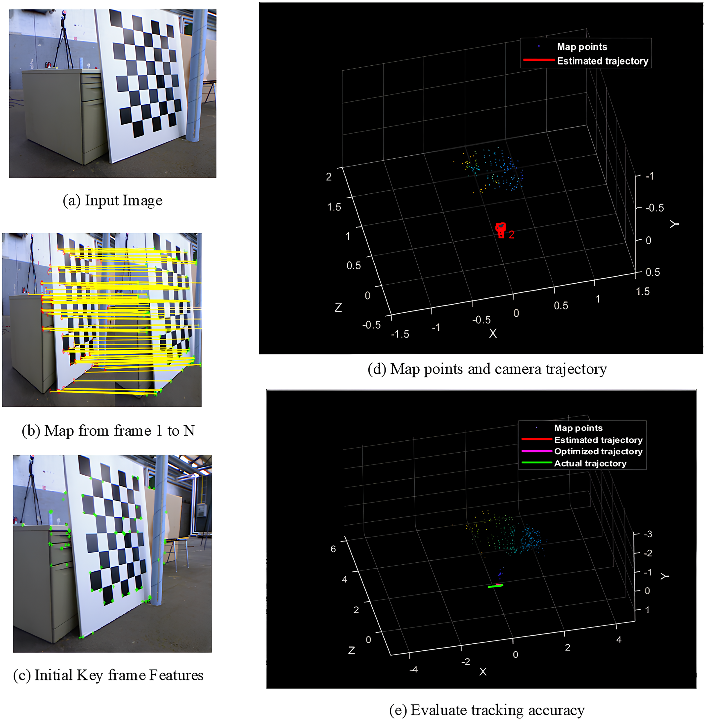
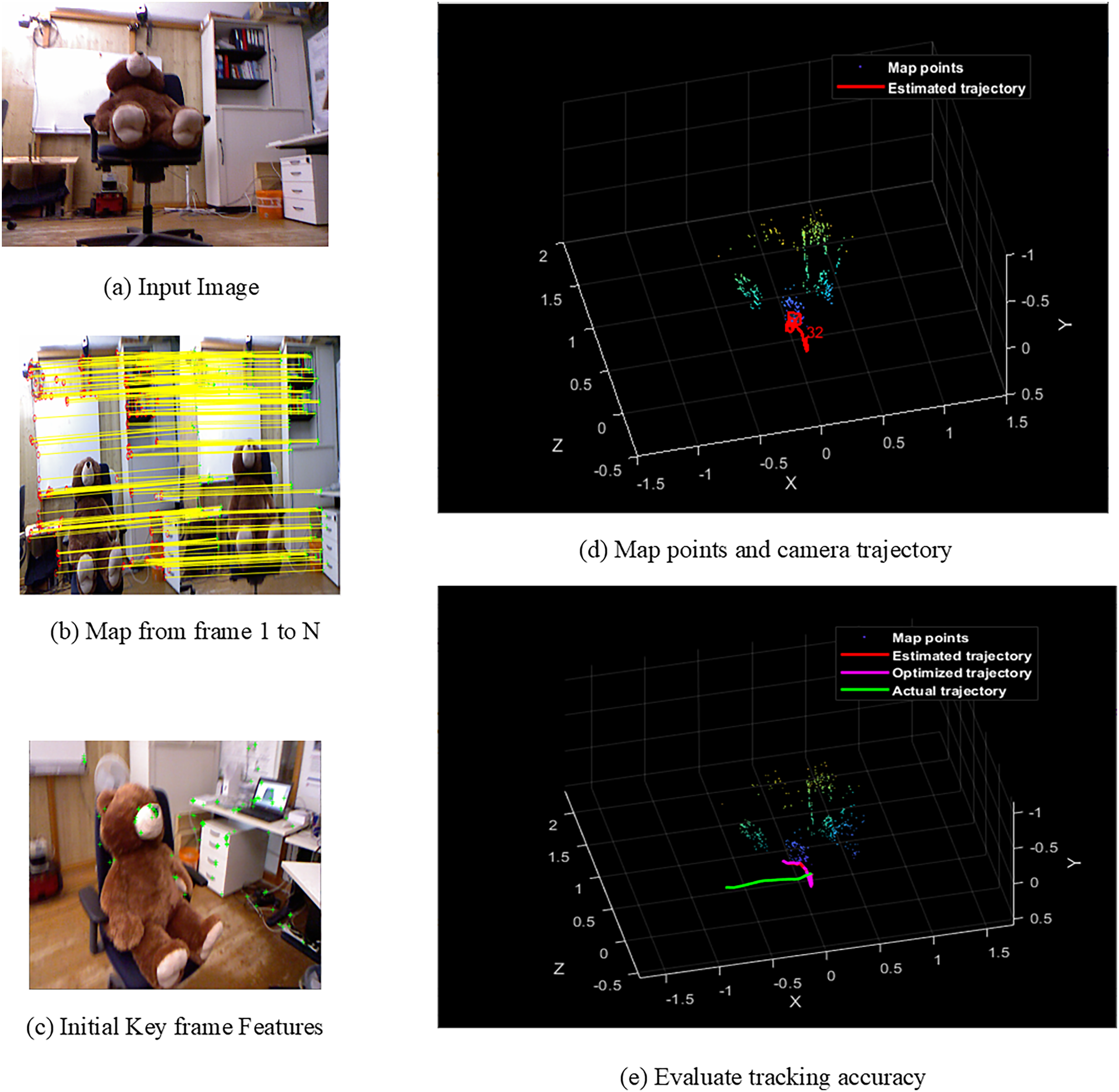
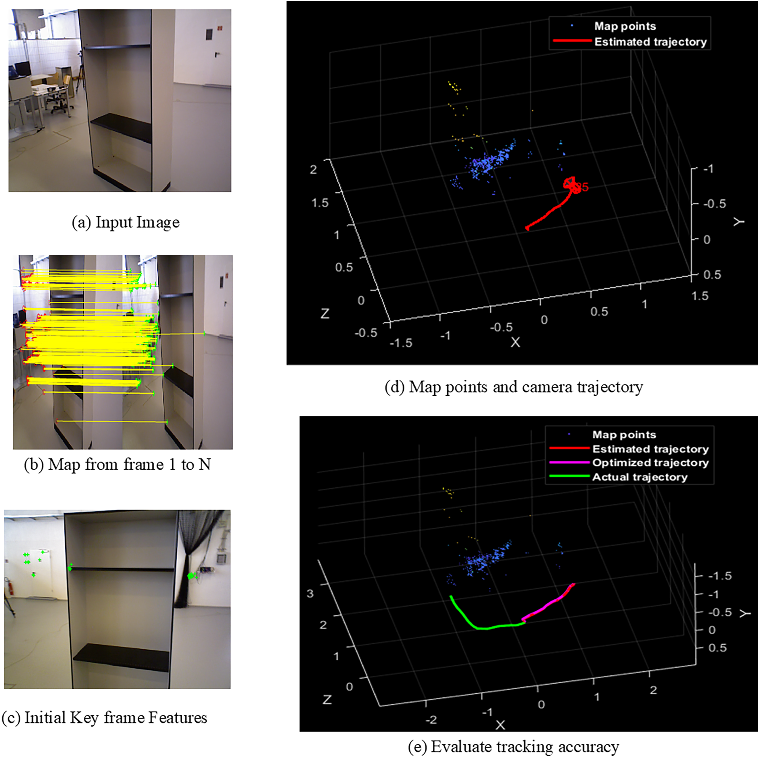
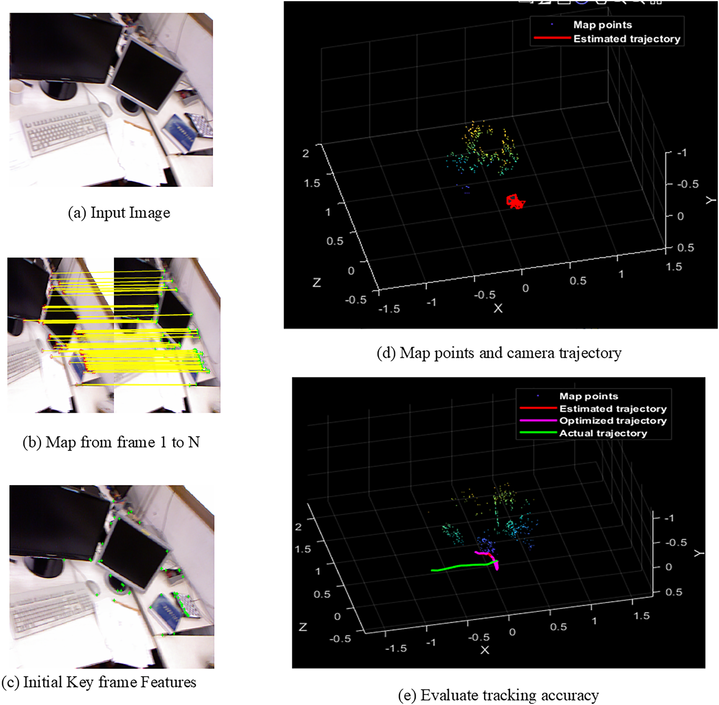
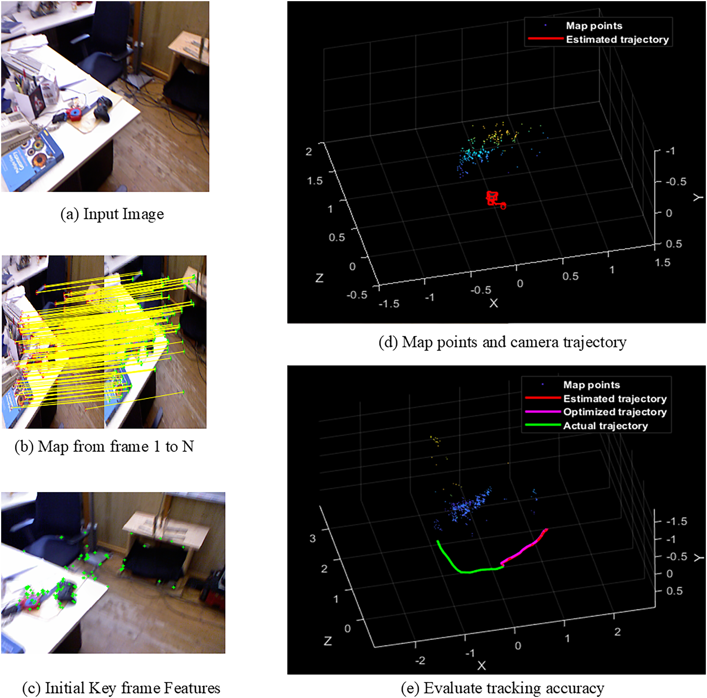
Figures 4A–4E shows the sample screens of pioneer_SLAM class with input sample, frames mapping from 1 to N, initial key frames extraction, map points and camera projector and final tracking accuracy. Figures 5A–5E shows the sample screens of teddy class with input sample, frames mapping from 1 to N, initial key frames extraction, map points and camera projector and final tracking accuracy. Figures 6A–6E shows the sample screens of cabinet class with input sample, frames mapping from 1 to N, initial key frames extraction, map points and camera projector and final tracking accuracy. Figures 7A–7E shows the sample screens of freiburg1_rpy class with input sample, frames mapping from 1 to N, initial key frames extraction, map points and camera projector and final tracking accuracy. Figures 8A–8E shows the sample screens of freiburg1_360_validation class with input sample, frames mapping from 1 to N, initial key frames extraction, map points and camera projector and final tracking accuracy.
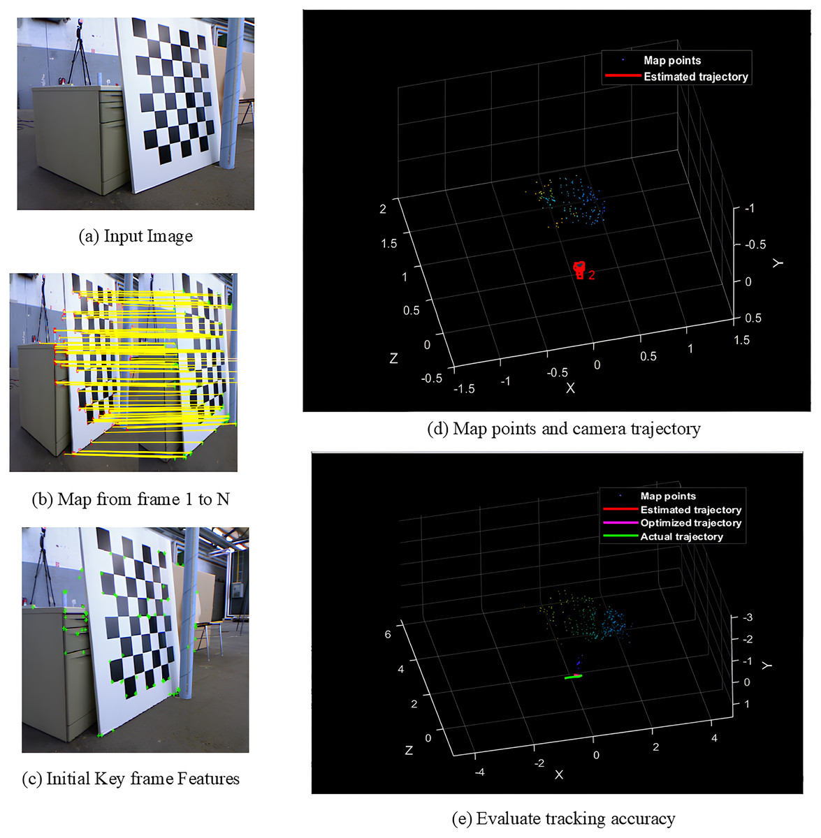
Figure 4: Screens of pioneer.
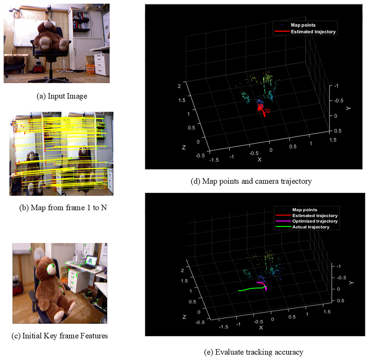
Figure 5: Screens of teddy.
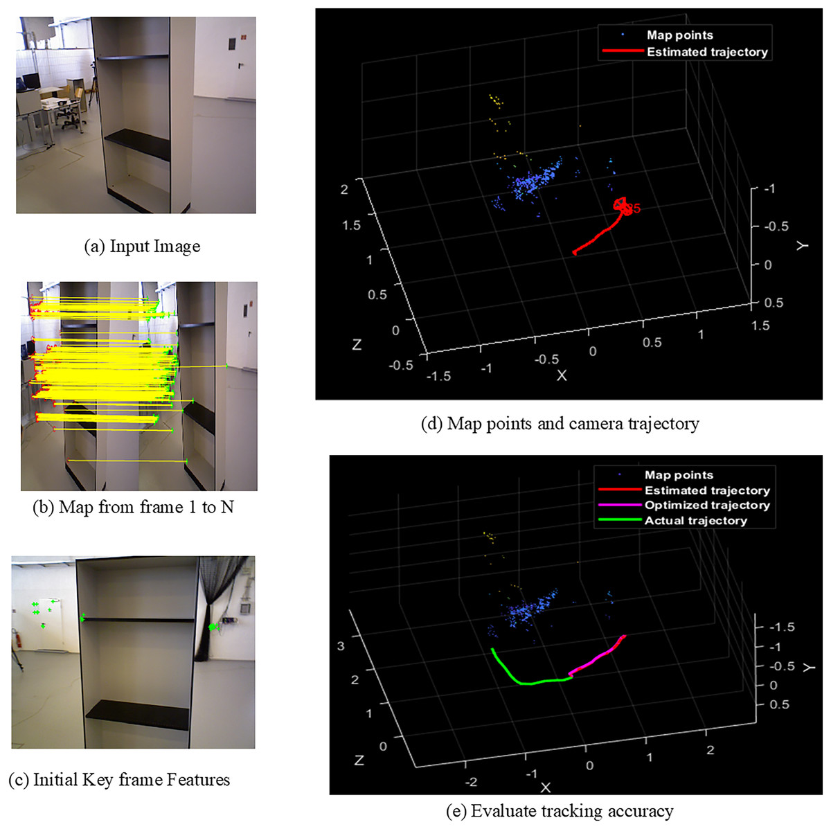
Figure 6: Screens of cabinet.
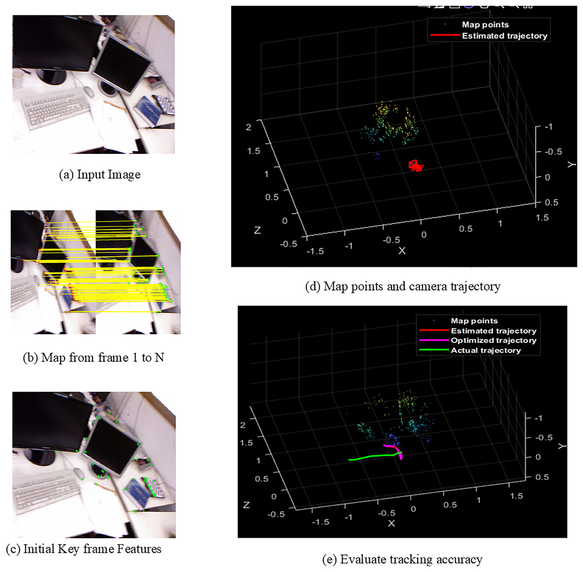
Figure 7: Screens of sitting.
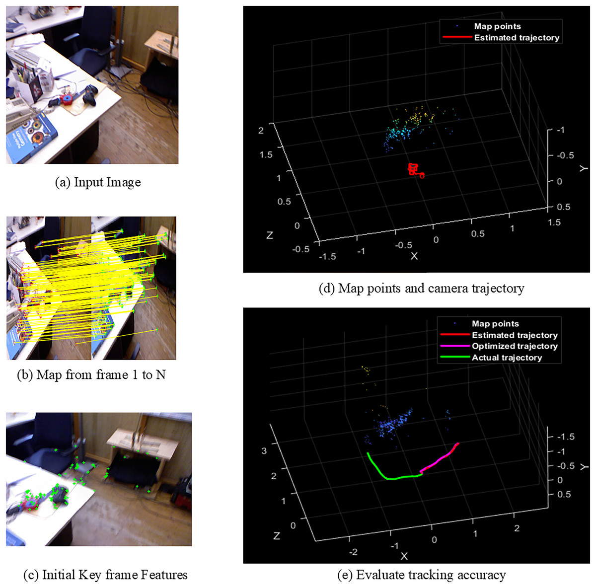
Figure 8: Screens of walking.
Tables 1 and 2 shows the performance comparison of APE, and RPE comparison against methods like DGS-SLAM, YOLO-SLAM, ORB-SLAM2, OPF-SLAM, DynaTM-SLAM, DI-SLAM, and EMFOA-OFT-SLAM for sitting, and walking datasets.
| Methods/metrics | rgbd_dataset_freiburg3_sitting_xyz | rgbd_dataset_freiburg3_walking_xyz | ||||||
|---|---|---|---|---|---|---|---|---|
| Mean (APE) (m) | Median (APE) (m) | RMSE (APE) (m) | StD (APE) (m) | Mean (APE) (m) | Median (APE) (m) | RMSE (APE) (m) | StD (APE) (m) | |
| DGS-SLAM | 0.3679 | 0.3641 | 0.3594 | 0.1387 | 0.3529 | 0.3456 | 0.3469 | 0.1471 |
| YOLO-SLAM | 0.3348 | 0.3469 | 0.3457 | 0.1271 | 0.3424 | 0.3285 | 0.3376 | 0.1369 |
| ORB-SLAM2 | 0.3155 | 0.3217 | 0.3261 | 0.1163 | 0.3275 | 0.3122 | 0.3247 | 0.1254 |
| OPF-SLAM | 0.2926 | 0.3025 | 0.2878 | 0.1047 | 0.2871 | 0.2965 | 0.3118 | 0.1148 |
| DynaTM-SLAM | 0.2651 | 0.2818 | 0.2653 | 0.0938 | 0.2523 | 0.2761 | 0.2975 | 0.1032 |
| DI-SLAM | 0.2418 | 0.2603 | 0.2365 | 0.0822 | 0.2249 | 0.2387 | 0.2847 | 0.0917 |
| EMFOA-OFT-SLAM | 0.2211 | 0.2359 | 0.2159 | 0.0716 | 0.2058 | 0.2192 | 0.2724 | 0.0808 |
| DGS-SLAM | 39.9021 | 35.2101 | 39.9276 | 48.3778 | 41.6831 | 36.5740 | 21.4759 | 45.0713 |
| YOLO-SLAM | 33.9605 | 31.9976 | 37.5470 | 43.6664 | 39.8948 | 33.2724 | 19.3127 | 40.9788 |
| ORB-SLAM2 | 29.9207 | 26.6708 | 33.7933 | 38.4350 | 37.1603 | 29.7885 | 16.1071 | 35.5661 |
| OPF-SLAM | 24.4360 | 22.0165 | 24.9826 | 31.6141 | 28.3176 | 26.0708 | 12.6363 | 29.6167 |
| DynaTM-SLAM | 16.5975 | 16.2881 | 18.6204 | 23.6670 | 18.4304 | 20.6084 | 8.4369 | 21.7054 |
| DI-SLAM | 8.5607 | 9.3738 | 8.7103 | 12.8953 | 8.4926 | 8.1692 | 4.3203 | 11.8869 |
| Methods/metrics | rgbd_dataset_freiburg3_sitting_xyz | rgbd_dataset_freiburg3_walking_xyz | ||||||
|---|---|---|---|---|---|---|---|---|
| Mean (RPE) (m) | Median (RPE) (m) | StD (RPE) (m) | RMSE (RPE) (m) | Mean (RPE) (m) | Median (RPE) (m) | StD (RPE) (m) | RMSE (RPE) (m) | |
| DGS-SLAM | 0.1982 | 0.0936 | 0.2254 | 0.3051 | 0.1892 | 0.1571 | 0.2542 | 0.2783 |
| YOLO-SLAM | 0.1894 | 0.0815 | 0.2015 | 0.2863 | 0.1713 | 0.1347 | 0.2215 | 0.2547 |
| ORB-SLAM2 | 0.1723 | 0.0746 | 0.1871 | 0.2718 | 0.1578 | 0.1154 | 0.2021 | 0.2368 |
| OPF-SLAM | 0.1632 | 0.0652 | 0.1431 | 0.1623 | 0.1251 | 0.1022 | 0.1876 | 0.2154 |
| DynaTM-SLAM | 0.1527 | 0.0537 | 0.1247 | 0.1462 | 0.1142 | 0.0917 | 0.1688 | 0.2013 |
| DI-SLAM | 0.1354 | 0.0426 | 0.1158 | 0.1305 | 0.1037 | 0.0804 | 0.1569 | 0.1891 |
| EMFOA-OFT-SLAM | 0.0915 | 0.0318 | 0.0926 | 0.1157 | 0.0914 | 0.0709 | 0.1257 | 0.1667 |
| DGS-SLAM | 53.8345 | 66.0256 | 58.9175 | 62.0780 | 51.6914 | 54.8696 | 50.5507 | 62.0780 |
| YOLO-SLAM | 51.6895 | 60.9816 | 54.0446 | 59.5878 | 46.6433 | 47.3645 | 43.2506 | 59.5878 |
| ORB-SLAM2 | 46.8949 | 57.3726 | 50.5078 | 57.4320 | 42.0786 | 38.5615 | 37.8030 | 57.4319 |
| OPF-SLAM | 43.9338 | 51.2270 | 35.2900 | 28.7122 | 26.9384 | 30.6262 | 32.9957 | 28.7122 |
| DynaTM-SLAM | 40.0786 | 40.7821 | 25.7417 | 20.8618 | 19.9650 | 22.6826 | 25.5331 | 20.8618 |
| DI-SLAM | 32.4224 | 25.3522 | 20.0345 | 11.3410 | 11.8611 | 11.8159 | 19.8852 | 11.3410 |
Table 3 shows the performance comparison of accuracy, and error comparison against methods like DGS-SLAM, YOLO-SLAM, ORB-SLAM2, OPF-SLAM,DynaTM-SLAM, DI-SLAM, and EMFOA-OFT-SLAM for sitting, and walking datasets. It shows that the proposed model has highest results of 92.82%, and 91.98% for sitting, and walking dataset. Proposed system also has lowest computation time of 23.72, and 32.69 ms for sitting, and walking.
| Dataset | rgbd_dataset_freiburg3_sitting_xyz (%) | rgbd_dataset_freiburg3_walking_xyz (%) | ||||
|---|---|---|---|---|---|---|
| Methods/metrics | Accuracy | Error | Time consumption (ms) | Accuracy | Error | Time consumption (ms) |
| DGS-SLAM | 86.11 | 13.89 | 45.21 | 85.18 | 14.82 | 47.65 |
| YOLO-SLAM | 87.26 | 12.74 | 40.59 | 86.25 | 13.75 | 44.18 |
| ORB-SLAM2 | 88.34 | 11.66 | 38.81 | 87.57 | 12.43 | 42.67 |
| OPF-SLAM | 89.51 | 10.49 | 33.56 | 88.73 | 11.27 | 40.54 |
| DynaTM-SLAM | 90.59 | 9.41 | 28.35 | 89.69 | 10.31 | 38.43 |
| DI-SLAM | 91.75 | 8.25 | 26.67 | 90.95 | 9.05 | 36.58 |
| EMFOA-OFT-SLAM | 92.82 | 7.18 | 23.72 | 91.98 | 8.02 | 32.69 |
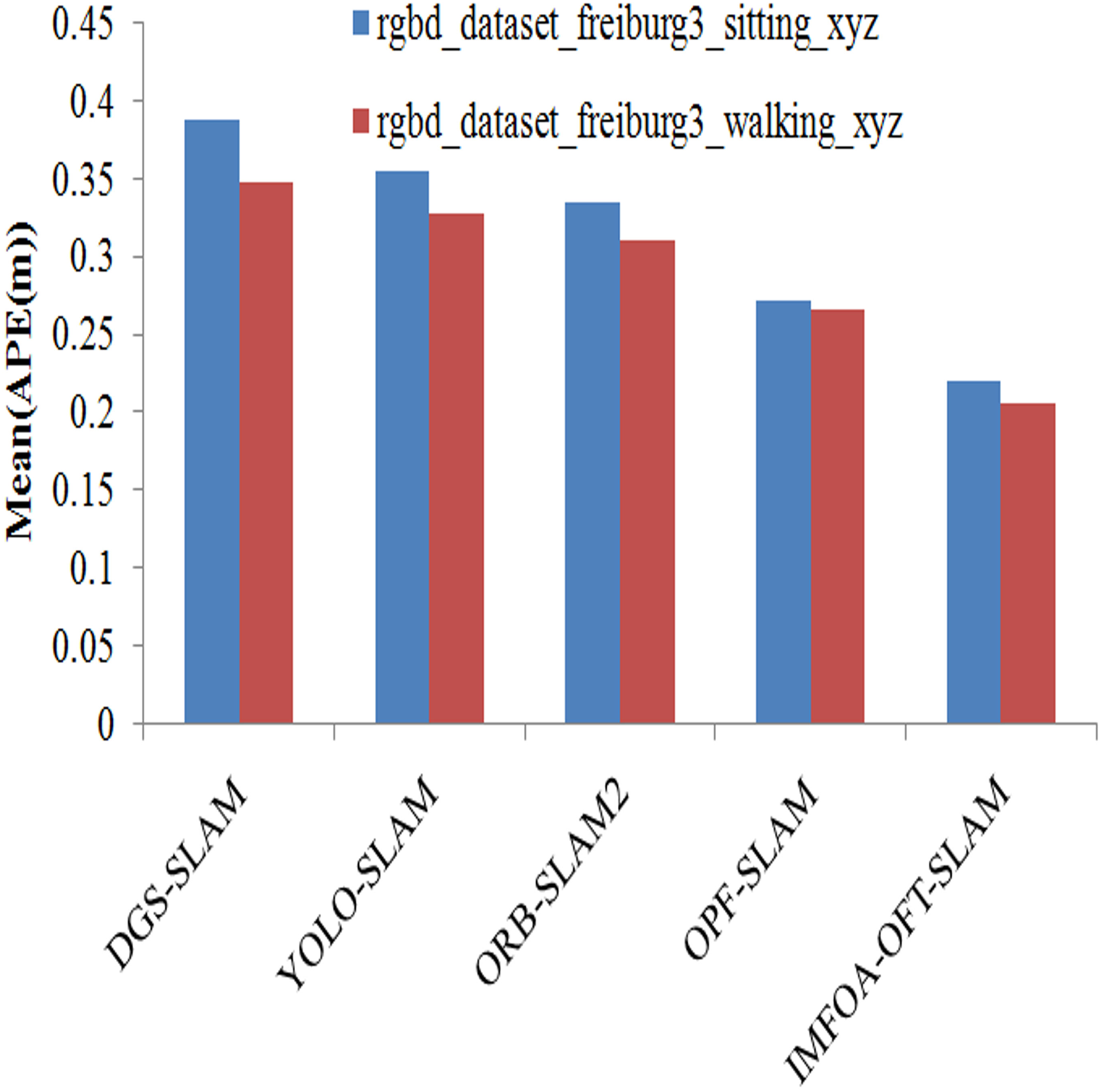
The experimental results of algorithms on mean results achieved by APE is illustrated in the Fig. 9. The results are measured by varying TUM RGB-D dataset from both walking and sitting. The suggested approach has the lowest mean APE for both types of activities compared to previous techniques. This system has the lowest mean APE of 0.2211, and 0.2058 for walking and sitting. The other methods such as DGS-SLAM, YOLO-SLAM, ORB-SLAM2, OPF-SLAM,DynaTM-SLAM, and DI-SLAM have the highest mean APE of 0.3679, 0.3348, 0.3155, 0.2926, 0.2651, and 0.2418 for sitting.
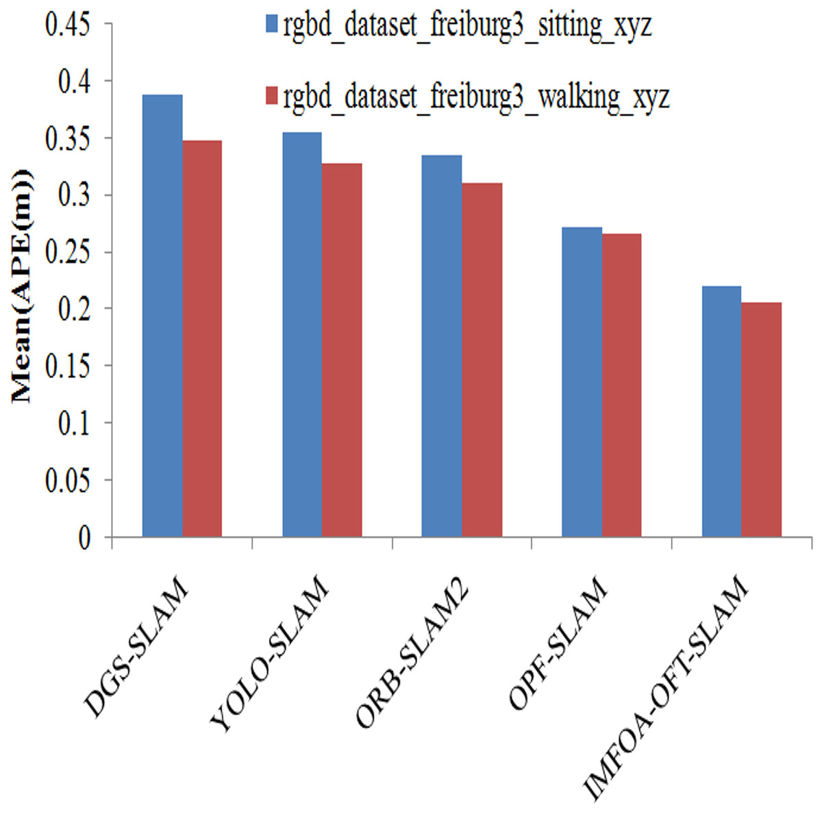
Figure 9: APE (mean) comparison of algorithms.
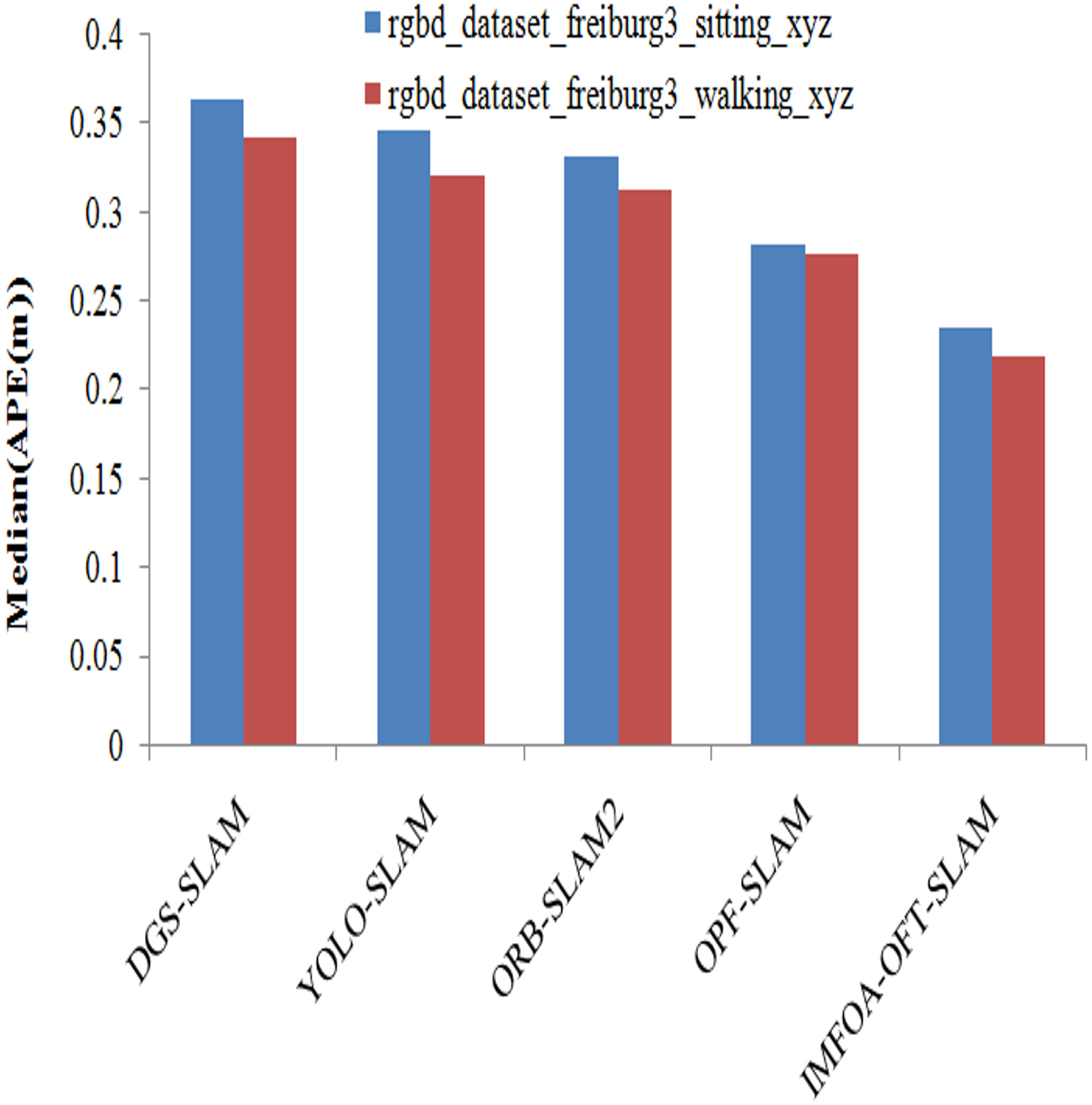
Median results achieved by APE among algorithms are illustrated in the Fig. 10. The median results are measured by varying TUM RGB-D dataset from both walking and sitting. The suggested approach has the lowest median APE for both types of activities compared to previous techniques. The proposed system has the lowest median APE of 0.2359, and 0.2192 for walking and sitting. The other methods such as DGS-SLAM, YOLO-SLAM, ORB-SLAM2, OPF-SLAM,DynaTM-SLAM, and DI-SLAM have the highest median APE of 0.3641, 0.3469, 0.3217, 0.3025, 0.2818, and 0.2603 for sitting.
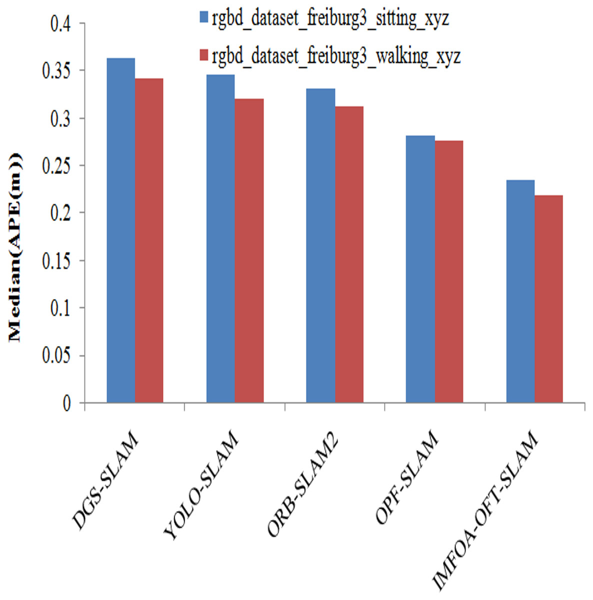
Figure 10: APE (Median) comparison of algorithms.
RMSE results achieved by APE among algorithms are illustrated in the Fig. 11. The RMSE results are measured by varying TUM RGB-D dataset from both walking and sitting. From the results it shows that the proposed system has lowest RMSE (APE) when compared to other methods on both types of actions. The proposed system has lowest RMSE (APE) of 0.2159, and 0.2724 for walking and sitting. The other methods such as DGS-SLAM, YOLO-SLAM, ORB-SLAM2, OPF-SLAM,DynaTM-SLAM, and DI-SLAM have the highest RMSE (APE) of 0.3594, 0.3457, 0.3261, 0.2878, 0.2653, and 0.2365 for sitting.
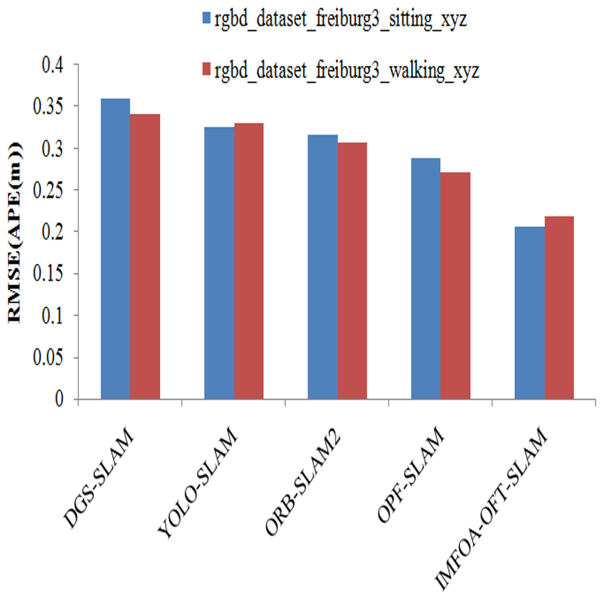
Figure 11: APE (RMSE) comparison of algorithms.
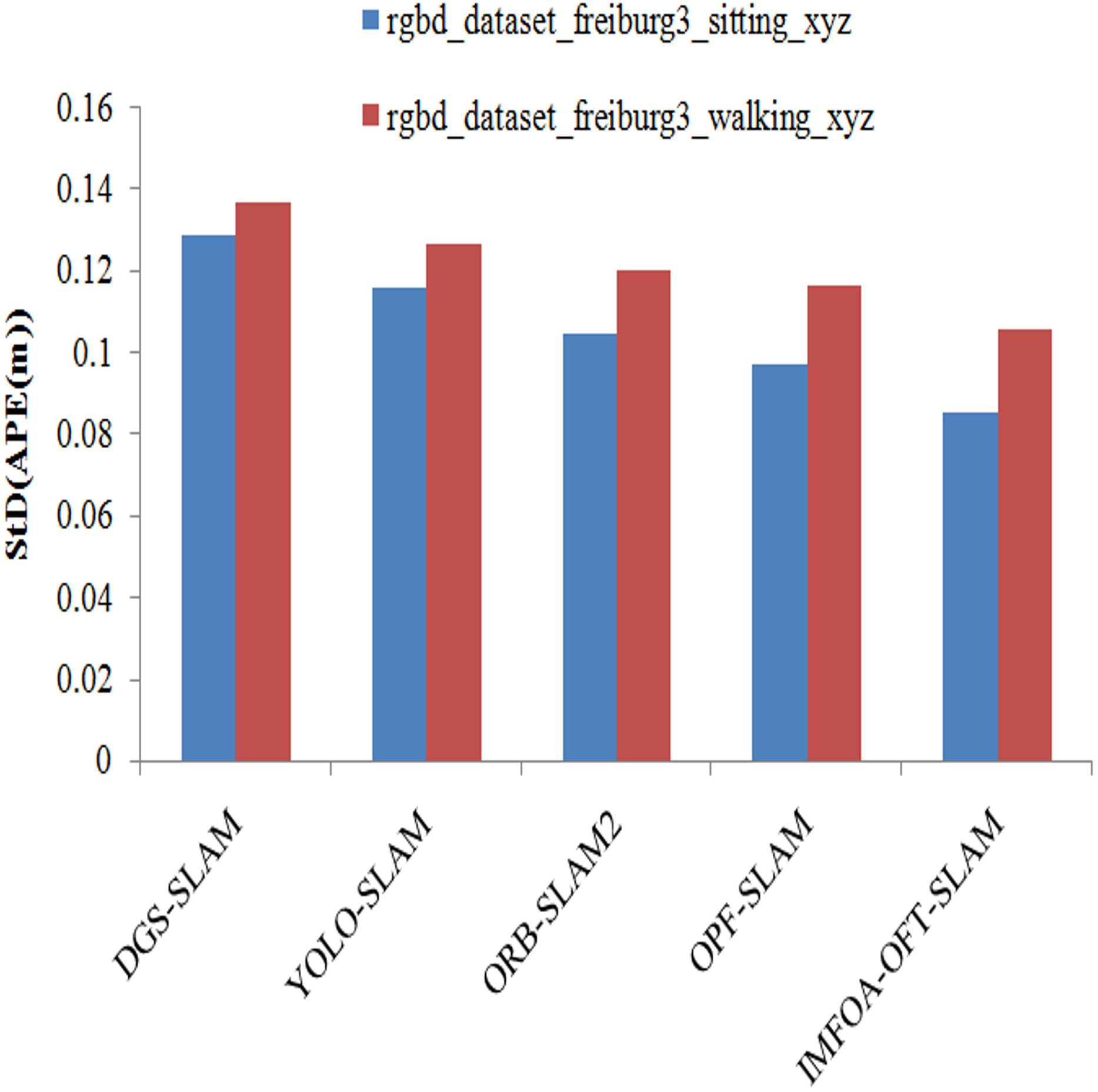
StD results achieved by APE among algorithms are illustrated in the Fig. 12. StD results are measured by varying walking and seated TUM RGB-D datasets. From the results it shows that the proposed system has lowest StD (APE) when compared to other methods on both types of actions. The proposed system has the lowest StD (APE) of 0.0716, and 0.0808 for walking and sitting. The other methods such as DGS-SLAM, YOLO-SLAM, ORB-SLAM2, OPF-SLAM,DynaTM-SLAM, and DI-SLAM have the highest StD APE of 0.1387, 0.1271, 0.1163, 0.1047, 0.0938, and 0.0822 for sitting.
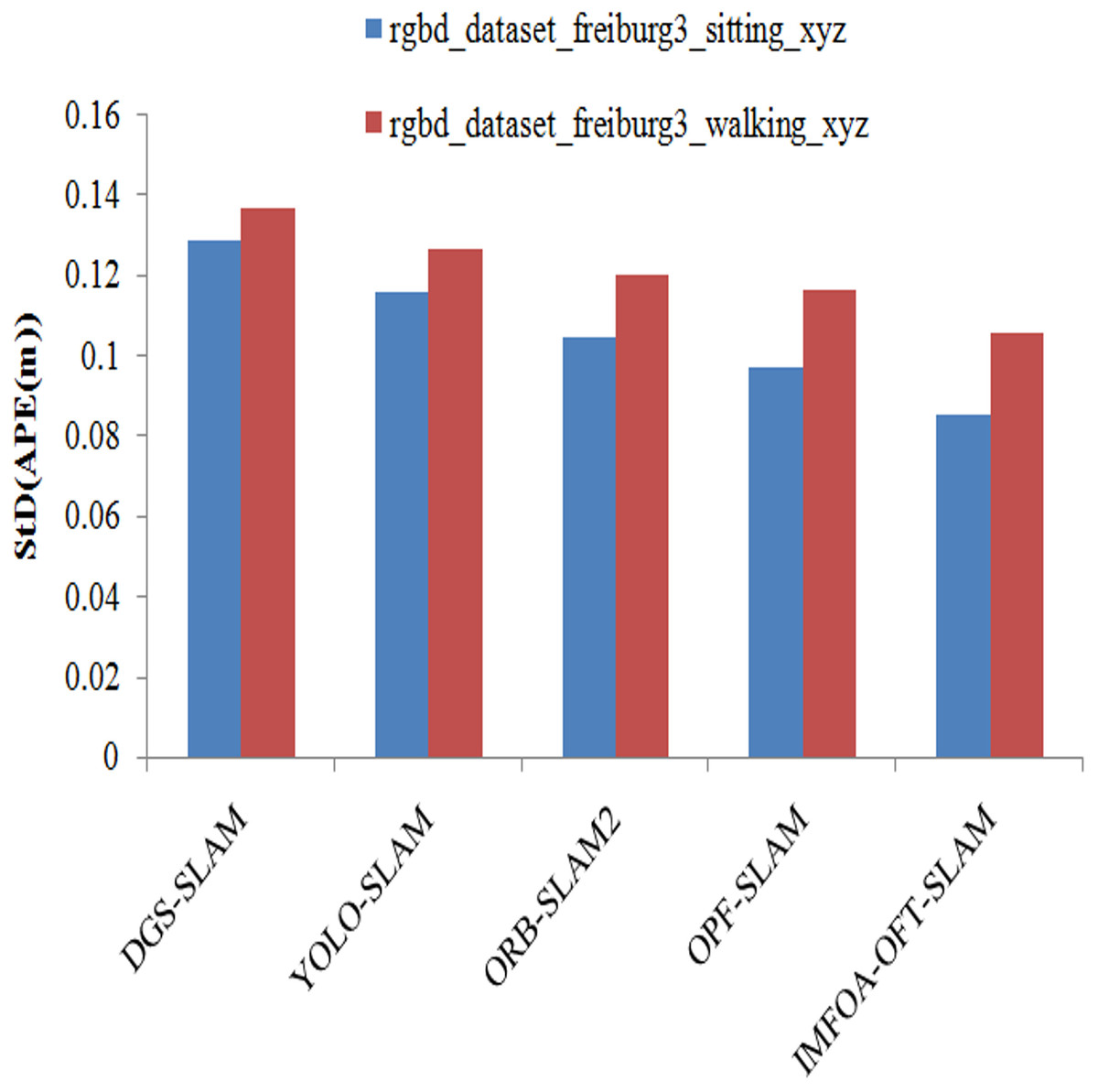
Figure 12: APE (StD) comparison of algorithms.
The procedures for preprocessing were as follows:
Temporal alignment of RGB and depth frames was achieved by RGB-D synchronization.
For the sake of computational consistency, we downsized all of the frames to a same resolution, such as 640 × 480.
We standardized the intensity data to the interval [0, 1].
Extracting Features: RGB frames were used to extract ORB key points. In which highly dynamic items were removed using an improved Mask R-CNN with a Cross-layer Feature Pyramid Network (CFPN), a technique known as semantic segmentation.
Assessment Approach: To test how well the suggested EMFOA-OFT SLAM system works and how accurate it is. Further, to assess the system’s accuracy, we contrasted the anticipated camera trajectories with the ground-truth trajectories from the TUM RGB-D dataset.
We captured and statistically examined frame-to-frame and cumulative pose differences.
Evaluation Criteria Total Posture Error (TPO) and finds the overall degree to which the forecasted path agrees with reality. The absolute position error (APE) is calculated over the entire flight. An RPE is a relative pose error, Evaluates the precision of motion from frame to frame at the local level. For testing precision in the near future, it works well because it is more affected by tiny changes.
Conclusion and future work
This study introduces a dynamic monocular visual SLAM system that minimizes dynamic objects in dynamic environment. An enhanced Mask R-CNN is proposed to more precisely segment very active items according to the SLAM algorithms in dynamic internal settings requirements in such scenes. Optical-Flow Tracking (OFT) using Daisy Filter Flow (DFF) is employed to match the remaining feature-point pairs. Elite Moth–Flame Optimization Algorithm (EMFOA), Cauchy distribution function is introduced for exploration, the best flame for exploitation, and adaptive step size to determine the optimal label field in DFF. DFF with a geometric approach provides an efficient method for dynamic object processing that eliminates very dynamic items from dynamic situations. Optical flow tracking with a fine-tuned Mask R-CNN, CFPN, and EMFOA enables dynamic object filtering and robust feature-point matching. TUM dynamic indoor environment dataset demonstrates comparable performance to other methods in low-dynamic environments. It shows that the proposed model has highest results of 92.82%, and 91.98% for sitting, and walking dataset. Proposed system also has lowest computation time of 23.72, and 32.69 ms for sitting, and walking. The TUM RGB-D dataset demonstrated substantial improvements in APE compared to other methods.
SLAM systems are trained on TUM RGB-D maynot perform well in outdoor datasets. The dataset does not include natural terrain, weather variations, or long-range depth sensing. The dataset was recorded in controlled indoor environments with stable illumination. It lacks examples of changing light, shadows, or glare. This issue has been solved by replacing traditional features (e.g., ORB, SIFT) with deep descriptors like SuperPoint/LightGlue, which are more resilient to lighting changes.
Normalize a comparison of the image’s brightness and contrast; reduce lighting-induced noise. Image gradients are used instead of raw pixel intensities for direct SLAM, improving robustness to shadows and glare. These descriptors are less sensitive to illumination changes which help to maintain tracking accuracy.
Currently, indoor RGB-D datasets are the only ones that have been used to test the system; its effectiveness in low-light or outdoor settings has not been evaluated.
There may be limitations on real-time applications on low-power devices due to the high GPU memory requirements of the Mask sR-CNN segmentation.
Potential avenues for further study include replacing a portable semantic segmentation network or in addition to the segmentation of semantics module, the system may be used to mask R-CNN. It increases accuracy, and error of model in dynamic environments.
Designing lightweight architecture for dynamic environments involves creating systems or structures that are adaptable, resource-efficient, and responsive to change in physical spaces, digital platforms, or robotic systems.
Advanced technologies like semantic SLAM, object detection, and multi-sensor fusion to maintain accuracy and robustness despite constant change in dynamic environments.