
Temporal and modal contributions to smartphone-based multimodal driving behavior classification: a comparative study of classical, deep learning, and patch-based time series transformer models
- Published
- Accepted
- Received
- Academic Editor
- Paulo Jorge Coelho
- Subject Areas
- Artificial Intelligence, Data Mining and Machine Learning, Mobile and Ubiquitous Computing, Spatial and Geographic Information Systems, Internet of Things
- Keywords
- Driving behavior, Smartphone sensing, OBD-II, Overpass API, Multimodal fusion, Deep learning, PatchTST
- Copyright
- © 2026 Sağbaş
- Licence
- This is an open access article distributed under the terms of the Creative Commons Attribution License, which permits unrestricted use, distribution, reproduction and adaptation in any medium and for any purpose provided that it is properly attributed. For attribution, the original author(s), title, publication source (PeerJ Computer Science) and either DOI or URL of the article must be cited.
- Cite this article
- 2026. Temporal and modal contributions to smartphone-based multimodal driving behavior classification: a comparative study of classical, deep learning, and patch-based time series transformer models. PeerJ Computer Science 12:e3493 https://doi.org/10.7717/peerj-cs.3493
Abstract
Understanding and classifying driving behavior is a critical component of modern intelligent transportation systems, with implications for traffic safety, fuel efficiency, and personalized driver support. As sensor-equipped mobile devices become increasingly pervasive, new opportunities have emerged for implementing data-driven behavior recognition systems in a cost-effective and accessible manner. This study presents a comprehensive and low-cost mobile framework for classifying driving behaviors using data collected entirely via a smartphone application. Unlike prior approaches that rely on embedded hardware, the proposed system performs all data acquisition and recording through a standard smartphone paired with a bluetooth-based on-board diagnostics II (OBD-II) adapter. The framework integrates multimodal sensor sources, including engine control unit (ECU) data, inertial motion sensors, enriched road metadata via the Overpass application programming interface (API), and environmental audio signals. Rather than isolating a single data domain, the system unifies mechanical, contextual, and behavioral dimensions to enable robust driving style analysis. Driving behavior was categorized into three classes (calm, normal, aggressive) using sliding time windows of 3, 5, 7, and 9 s. The effects of both window duration and data source composition on model performance were thoroughly evaluated. Classical machine learning models (artificial neural network (ANN), support vector machine (SVM), logistic regression (LR), Naive Bayes (NB)) based on engineered features were compared against deep learning architectures (convolutional neural network (CNN), long short-term memory (LSTM), gated recurrent unit (GRU), recurrent neural network (RNN)) trained on raw multivariate sequences. Results showed that multimodal integration substantially improved classification accuracy, with CNN achieving the highest performance. Additionally, the study incorporated patch-based time series transformer (PatchTST), a modern transformer-based architecture designed for time-series classification, across 128 experimental configurations. While CNN remained the top performer in overall accuracy, PatchTST yielded consistently stable and competitive results, particularly in long-window and feature-rich settings. Importantly, statistical analyses confirmed the significance of differences across feature sets, time windows, and model types. This included architectural parameters such as model depth and latent dimensionality, evaluated through analysis of variance (ANOVA) and post-hoc Tukey’s honestly significant difference (HSD) tests. By enabling high-accuracy driving behavior classification using only smartphone-based sensing, this study contributes a practical and scalable solution. The inclusion of attention-based PatchTST modeling further extends the methodological breadth, highlighting the role of transformer architectures in multivariate time-series analysis. Collectively, these contributions underscore the feasibility of deploying robust and intelligent driver monitoring systems in real-world environments.
Introduction
The electronic control unit (ECU) serves as the central intelligence of modern vehicles, regulating and optimizing nearly all automotive functions through an extensive network of embedded sensors. A diagnostic interface known as the on-board diagnostics (OBD) scanner can be connected to the vehicle’s ECU via the OBD port, enabling real-time access to vehicle data. Through the OBD protocol, individual subsets of sensor signals are identified, allowing for the retrieval and analysis of the ECU’s stored information. Consequently, any OBD-compliant vehicle provides access to a standardized set of diagnostic parameters, facilitating monitoring and analysis of vehicular performance; however, access to extended or manufacturer-specific signals may vary depending on proprietary restrictions and protocol implementations. Key sensors integrated within the ECU framework include emission sensors, vehicle speed sensors, revolutions per minute (RPM) sensors, throttle position sensors, fuel level sensors, and ambient temperature sensors. These ECUs and OBD interfaces are fundamental to capturing real-time driving data, making them essential tools for performance analysis, fault detection, and intelligent transportation system applications (Malik & Nandal, 2023). However, despite the critical role of ECU and OBD systems, existing studies often limit their scope to single data sources or handcrafted features, and rarely integrate them into cost-effective, multimodal frameworks. This shortcoming underlines the necessity for approaches that connect ECU data with other modalities in order to achieve more generalizable and scalable driving behavior analysis.
Driving behavior is a key determinant of both traffic safety and the efficiency of traffic flow. In the intricate traffic ecosystem comprising drivers, vehicles, and road infrastructure, human factors remain the predominant cause of traffic accidents (Miyaji, Danno & Oguri, 2008). Studies indicate that human error accounts for over 70% of traffic accidents, particularly during long-distance travel, where the driving environment becomes increasingly complex (Aufrère et al., 2003). Under such conditions, driver fatigue and emotional distress can lead to risky driving behaviors, further exacerbating road safety concerns. Simultaneously, vehicle intelligence and personalized driver assistance are emerging as key trends in the evolution of automotive technology. Predictive models tailored to individual driving habits hold significant potential in enhancing safety and user experience (Zou et al., 2022). Additionally, ensuring the optimal performance and efficiency of a vehicle during operation necessitates continuous monitoring of the internal combustion engine. Neglecting this can result in mechanical failures, reduced engine lifespan, increased fuel consumption, and heightened gas emissions. By leveraging real-time ECU data, engineers can monitor critical engine parameters throughout the vehicle development process, thereby enhancing reliability and performance (Bedretchuk et al., 2023). In this context, data-driven methodologies are increasingly being applied to engine diagnostics and vehicle dynamics to enhance driver interaction, provide real-time feedback, and extract valuable insights from vehicle systems. These advancements contribute to key industrial processes such as engine calibration, emissions regulation, and fuel efficiency optimization (Claßen et al., 2021; Canal, Riffel & Gracioli, 2024). Nevertheless, most existing studies emphasize either safety outcomes or mechanical optimization in isolation, without adequately linking these factors to comprehensive behavior modeling. This gap highlights the importance of multimodal, smartphone-based approaches that simultaneously address driver, vehicle, and environmental dimensions.
In driving behavior research, the algorithms used to analyze driving patterns are inherently unique, each offering distinct advantages. The term driving behavior encompasses a novel framework for monitoring and recording numerous variables derived from a driver’s interaction with the vehicle and their driving habits. As research in this field continues to evolve, the development of effective and error-free evaluation models remains essential. Machine learning and artificial intelligence play a pivotal role in these processes, significantly enhancing the accuracy and reliability of driving behavior analysis. These technologies are of paramount importance to automotive manufacturers, enabling optimization across various domains, including vehicle design, production, quality management, safety enhancement, and cost-effective after-sales services. By selecting the most relevant features from OBD data and leveraging appropriate machine learning algorithms, highly precise driving behavior estimations can be achieved, contributing directly to improved road safety. Standardized driving models can be constructed by integrating data from different vehicles’ OBD systems, thereby facilitating comprehensive behavioral assessments. Modern vehicles are now equipped with advanced internal databases capable of real-time driver monitoring. These systems can issue warnings or alerts based on detected driving behaviors, classifying them into categories such as normal or safe driving, aggressive driving, reckless driving, and high-risk behaviors such as impaired or intoxicated driving (Malik & Nandal, 2023). Yet, despite these advancements, many approaches remain constrained to conventional algorithms and limited sensing strategies, leaving more sophisticated architectures and richer multimodal integrations comparatively underexplored. This underutilization points to the need for further methodological innovation, which is taken up in the present study.
Literature review on driving behavior classification
In recent years, research on the classification of driving behaviors has expanded rapidly, with various approaches utilizing different data sources and methodologies. Studies in the literature frequently employ OBD-II data, motion sensors such as accelerometers and gyroscopes, global positioning system (GPS)-based location data, and machine learning techniques to analyze driving behavior.
Andria et al. (2016) developed a low-cost data collection platform for automotive telemetry applications, including driving style analysis, fleet management, and fault detection. Lattanzi & Freschi (2021) applied support vector machine (SVM) and neural networks to classify safe and unsafe driving using in-vehicle sensor data. Malik & Nandal (2023) analyzed OBD-II signals to distinguish between safe and reckless driving, while Singh & Singh (2022) combined ECU and accelerometer data to classify driving behaviors into categories such as bad, normal, and aggressive. Kumar & Jain (2023) modeled ten driving styles based on fuel consumption, steering, speed, and braking patterns, utilizing OBD-II data without requiring additional sensors. Ameen et al. (2021) continuously recorded speed, RPM, throttle, and load to categorize driving behaviors into safe, normal, aggressive, and dangerous classes. Zou et al. (2022) predicted vehicle acceleration using features such as distance, speed, and acceleration, while Azadani & Boukerche (2022) reviewed driving behavior studies by data type, objectives, and modeling techniques. Liu, Wang & Qiu (2020) introduced a motion-capture-based system employing multiple miniature inertial measurement units (IMUs) for real-time driver motion tracking. Cendales, Llamazares & Useche (2023) examined links between driving stress and risky behavior. Martinelli et al. (2020) used controller area network (CAN) bus and OBD-II data to classify driving styles, achieving 99% accuracy in identifying drivers.
Recent studies have also focused on fuel efficiency and driver categorization. Rastegar et al. (2024) analyzed driving patterns based on fuel consumption and powertrain variables such as acceleration and deceleration. Canal, Riffel & Gracioli (2024) applied machine learning to ECU data for fuel efficiency classification and consumption prediction. Mohammed et al. (2023) designed an electronic card system for remote vehicle monitoring. Yen et al. (2021) used deep learning with a universal OBD-II module supporting various CAN standards to analyze fuel use under different conditions. Fafoutellis et al. (2023) investigated the impact of the COVID-19 on driving behavior, identifying three main profiles: aggressive, eco, and typical.
Several studies have focused on electric and hybrid vehicles. Lee & Yang (2023) analyzed OBD-II data from electric and hybrid vehicles using deep learning. Pirayre et al. (2022) studied behavior across road types (e.g., urban vs. highway) with GPS-based Markov chain modelling, while Lin, Zhang & Chang (2023) combined geographic data with OBD-II and CAN bus recordings to extract image-based driving patterns. Zhang & Lin (2021) integrated video, road signs, and GPS data to identify critical visual indicators of driving behavior.
Advancements in deep learning and artificial intelligence have further improved classification accuracy. Merenda et al. (2022) trained convolutional neural network (CNN) models, while Yarlagadda & Pawar (2022) analyzed real-time performance features, and Li, Lin & Chou (2022) evaluated risky driving using fuzzy inference systems and long short-term memory (LSTM) networks. Al-Rakhami et al. (2021) proposed an edge-fog-cloud deep learning frameworks that improved efficiency and accuracy 1.84%. Tripicchio & D’Avella (2022) combined Bayesian network with long short-term memory (LSTM) and SVM, achieving 92% accuracy for advanced driver assistance systems (ADAS) application. Fadzil et al. (2026) analyzed online OBD-II datasets from Kaggle to identify driver groups based on driving styles. Lastly, Fattahi, Golroo & Ghatee (2023) developed a smartphone-based system for detecting aggressive maneuvers using speed, RPM, and accelerometer data, demonstrating the feasibility of cost-effective driver monitoring.
Research gaps in driving behavior analysis
A holistic examination of recent studies on driving behavior analysis through engine operations reveals several gaps in the literature. Some studies (Andria et al., 2016; Ameen et al., 2021; Mohammed et al., 2023; Pirayre et al., 2022; Lin, Zhang & Chang, 2023; Zhang & Lin, 2021) incorporate GPS sensors; however, their usage is often limited to acquiring only speed and location data, overlooking other potential insights that could be derived from GPS-based analysis. Additionally, several studies utilize intermediate hardware components such as Raspberry Pi (Andria et al., 2016), Arduino (Singh & Singh, 2022), peripheral interface controller (PIC) microcontrollers, and ESP32 modules (Ameen et al., 2021; Mohammed et al., 2023) to record, store, and process ECU data. While these external devices facilitate data acquisition, their integration introduces higher costs and installation complexities compared to smartphones. Given that smartphones are widely used, equipped with multiple built-in sensors, and offer seamless data connectivity, leveraging them for driving behavior analysis presents a cost-effective and practical alternative to dedicated hardware solutions.
To address the limitations identified in existing research, this study expands the use of GPS data beyond speed and location by incorporating additional contextual features such as road type, speed limit, number of lanes, and road surface conditions via the Overpass application programming interface (API). This enhancement allows for a more comprehensive evaluation of driving behaviors by considering not only vehicle dynamics but also environmental factors. Furthermore, unlike previous studies that rely on external hardware for ECU data acquisition, this research collects data directly through a smartphone and an OBD-II connection. This approach eliminates the need for additional recording devices, reducing both cost and installation complexity. Additionally, by leveraging built-in smartphone sensors (such as the accelerometer, gyroscope, and magnetometer) as well as environmental audio signals, driving behavior analysis becomes more robust and multidimensional. Ultimately, this study introduces a cost-effective and scalable driving behavior analysis model that integrates multiple data sources, providing a more comprehensive and accessible alternative to existing systems.
Moreover, while numerous studies have explored traditional machine learning algorithms and basic deep learning architectures such as CNNs and recurrent neural networks (RNNs) for driving behavior classification, there remains a noticeable gap in the application of more recent and advanced sequence modeling techniques. In particular, transformer-based models that leverage attention mechanisms (such as vision transformers (ViT), temporal fusion transformers (TFT), and PatchTST) have not been extensively adopted in this domain. These models offer significant advantages in capturing long-range temporal dependencies and complex multimodal interactions, which are critical for accurately characterizing dynamic driving behaviors. The lack of utilization of such architectures in prior research highlights a methodological gap that this study aims to address through the integration and comprehensive evaluation of attention-based models in driving behavior analysis.
Limitations and optimization strategies
One of the primary limitations of this study is the high computational demand required to process data from motion sensors and audio signals. In particular, the extraction of frequency-based features from audio signals and the continuous processing of motion data imposes significant computational costs on mobile devices. Additionally, the reliance on the Overpass API, which plays a crucial role in enriching GPS data, necessitates an active internet connection, potentially limiting the system’s usability in offline environments. Moreover, transformer-based models such as PatchTST, while offering improved temporal modeling capabilities, typically require large amounts of data and computational resources to achieve optimal performance. This can pose further challenges for real-time deployment on resource-constrained platforms such as mobile devices.
Another important limitation concerns the taxonomy employed in this study, which was restricted to three categories. While real-world driving behavior encompasses additional conditions such as distraction, drowsiness, reckless maneuvers, or eco-driving, these could not be reliably incorporated without additional modalities (e.g., driver-facing cameras, eye-tracking) and standardized labeling procedures. The present taxonomy should therefore be regarded as a baseline that can be practically deployed with smartphone-only sensing, while also remaining extendable to finer-grained states in future investigations.
A further limitation is that the experimental design was restricted to short-window benchmarks conducted on data collected from a single vehicle and driver. Cross-driver, cross-vehicle, and cross-environment validation (essential for assessing model generalizability) were not performed due to dataset constraints. Similarly, aspects such as robustness to sensor noise, computational energy efficiency on mobile platforms, and interpretability of deep and transformer-based models were not addressed in the current study. These omissions limit immediate deployment potential but provide a clear direction for subsequent investigations.
To mitigate these challenges, several optimization strategies can be implemented. Adjusting data refresh frequencies, employing longer window intervals in classification processes, and performing less frequent but more comprehensive analyses over extended time periods can help reduce computational load. These approaches not only enhance the system’s efficiency on mobile devices but also contribute to the sustainability of real-time analysis by balancing performance and resource utilization.
Proposed approach and contributions
This study introduces a novel, cost-effective, and multimodal framework for driving behavior classification by leveraging the synergy between vehicle ECU data, smartphone-based motion sensors, GPS-derived road metadata, and environmental audio signals. Unlike many prior works that rely on external microcontrollers, limited sensor inputs, or handcrafted features, the proposed system emphasizes accessibility, scalability, and real-time analysis through a unified mobile application platform.
The core innovation of this study lies in its seamless integration of four distinct sensor domains: (1) engine operational data via the OBD-II interface, (2) inertial motion data from accelerometer, gyroscope, gravity, and magnetometer sensors, (3) contextual road information retrieved dynamically from the Overpass API, and (4) spectral and statistical features extracted from environmental sound recordings. This diverse sensor fusion enables the system to capture not only vehicle and driver dynamics but also environmental and contextual cues, leading to a more holistic assessment of driving behaviors.
The present study was designed to address style-level driving behavior rather than cognitive driver states. A coarse-grained taxonomy was selected to align with the modalities available from a smartphone-centric sensing pipeline and to ensure reliable labeling. Categories such as distracted or drowsy usually require driver-facing measurements (e.g., gaze or eyelid closure) and standardized annotation protocols; incorporating such states without the appropriate modalities would risk label noise and construct conflation. Consequently, the three-class taxonomy is positioned as an extendable foundation for telematics applications, compatible with future refinements once additional sensing and validated ground-truth resources become available.
This study is driven by the following research questions: (1) To what extent can smartphone-centric multimodal sensing provide reliable classification of driving behaviors? (2) How do classical machine learning, deep learning, and transformer-based models compare in terms of accuracy and robustness across different temporal window lengths and feature subsets? (3) What is the incremental contribution of each sensing modality to overall classification performance? These questions structure the experimental design and guide the interpretation of findings.
To represent these multimodal signals, the study proposes two complementary data preparation pipelines: one for classical machine learning and another for deep learning. In the classical pipeline, 66 handcrafted features were engineered from motion, engine, road, and audio signals using statistical and domain-specific descriptors. In contrast, the deep learning and PatchTST pipeline preserved the raw temporal structure of sensor streams, forming T × 37 matrices from time-windowed segments of raw data (with T varying according to the selected window duration). This dual approach enabled a comparative analysis of performance across traditional and modern classification paradigms.
Crucially, the study systematically evaluated the effects of time window length (3, 5, 7, and 9 s) and feature subset composition (ranging from ECU-only data to full sensor fusion) on classification performance. By structuring the dataset into 16 experimental configurations (spanning all combinations of window lengths and feature subsets) fine-grained insights were obtained regarding the temporal resolution required for accurate behavior modeling and the incremental benefit of adding each sensor modality. The impact of these variables was not only evaluated through performance metrics (accuracy, precision, recall, F1-score, area under the curve (AUC)), but also substantiated with detailed statistical comparisons between configurations, providing robust evidence of the performance gains resulting from longer window durations and multimodal integration. This study advances the field by introducing a smartphone-centric multimodal framework that unifies OBD-II data, motion sensing, enriched road metadata, and environmental audio into a single dataset. Unlike prior work relying on limited modalities or external devices, the present design enables cost-effective, scalable data acquisition. Furthermore, by systematically comparing classical machine learning (ML), deep learning, and attention-based transformer models, the study provides one of the first evaluations of transformer architectures for multimodal driving behavior analysis. This combination of modality integration, smartphone-based deployment, and advanced modeling establishes a new benchmark for future research in intelligent transportation systems. The major contributions of this study are summarized as follows:
-
Standardized multimodal dataset construction: This study introduces one of the first smartphone-centric multimodal datasets that combines ECU, motion, road metadata, and audio in a standardized collection framework.
-
Dynamic road context integration via Overpass API: By leveraging the Overpass API, the study dynamically retrieves contextual road metadata (such as speed limits, road type, lane count, one-way status, surface condition, and toll information) for each GPS trace.
-
Systematic evaluation of temporal granularity: Driving sequences were segmented into sliding windows of 3, 5, 7, and 9 s to explore the effect of temporal resolution on classification performance.
-
Comprehensive benchmarking of classical and deep learning models: The study compares engineered-feature-based classical models (SVM, LR, NB, ANN) with raw-sequence-based deep learning architectures (CNN, RNN, LSTM, GRU).
-
Modal contribution analysis across sensor domains: The individual and joint effects of motion sensors, road metadata (from Overpass), and environmental audio signals on classification accuracy are systematically assessed.
-
Integration of time and frequency domain audio features: Thirteen handcrafted audio features (spanning both time and spectral domains) were extracted from environmental sound recordings to capture subtle contextual cues (e.g., road noise, acceleration intensity).
-
Cost-effective and scalable mobile-based acquisition pipeline: The entire system runs on a consumer-grade Android smartphone connected to a low-cost OBD-II Bluetooth adapter, eliminating the need for microcontrollers like Raspberry Pi or Arduino.
-
Integration and evaluation of advanced Transformer-based architectures (PatchTST): This study pioneers the integration of PatchTST, a state-of-the-art transformer-based time-series classification model utilizing patch-level attention mechanisms, into the domain of driving behavior analysis.
Through these contributions, the proposed approach advances the field of intelligent transportation systems by demonstrating that low-cost, mobile-sensor-driven architectures can achieve high accuracy in driving behavior classification when supported by multimodal fusion, window-aware modeling, and statistically validated experimental designs.
System architecture and data acquisition
This section presents a comprehensive description of the system architecture and the data acquisition framework implemented in this study. It details the use of an ELM327 bluetooth device for retrieving real-time vehicle data from the OBD-II interface. In addition, the section describes how motion-related signals are continuously recorded using the smartphone’s built-in sensors. Environmental audio is also captured through the smartphone’s microphone. Furthermore, the system utilizes the phone’s GPS module to collect geospatial data. Together, these components constitute a multimodal sensing infrastructure, and the section provides a detailed explanation of how these heterogeneous data streams are acquired, synchronized, and stored using the custom-developed mobile application.
Sensor framework
Sensor axes enable the data obtained from different sensors to be represented within a static reference frame, relative to the physical location of the device. The Android sensor API defines this coordinate system based solely on the natural orientation of the device’s screen. Notably, the sensor axes remain fixed even if the screen orientation of the device changes (Android, 2025). Figure 1 illustrates the coordinate system utilized by the Android sensor API.
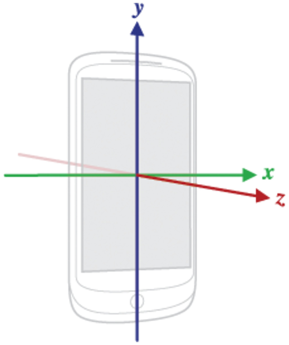
Figure 1: Coordinate system used by Sensor API for mobile devices (Android, 2025).
Accelerometer
The accelerometer measures acceleration along the X, Y, and Z axes in units of G (9.81 m/s2), capturing both linear acceleration and gravitational force (Sağbaş, Korukoglu & Balli, 2020). Figure 2 illustrates variations in Z-axis acceleration across calm, normal, and aggressive driving, demonstrating its utility for behavior discrimination.
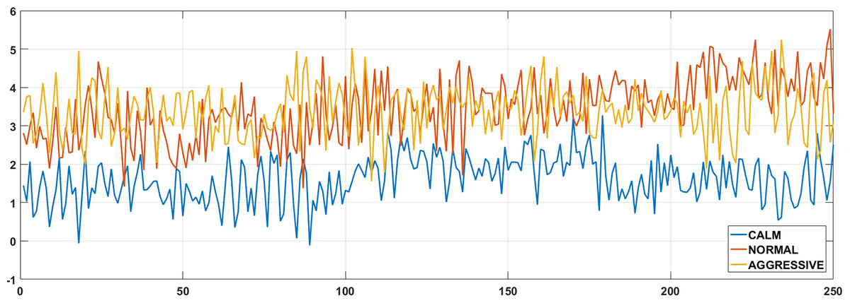
Figure 2: Example accelerometer Z-axis data for three different driving classes.
The linear acceleration sensor isolates motion by subtracting gravity from the accelerometer signal. When the device is stationary, its values should approach zero. Depending on hardware, it either fuses data from the gyroscope and accelerometer or, in the absence of a gyroscope, relies on accelerometer–magnetometer combinations (Android, 2025). The gravity sensor outputs the direction and magnitude of Earth’s gravity. Like the linear acceleration sensor, its calculation depends on device hardware, using either gyroscope–accelerometer fusion or accelerometer–magnetometer data (Android, 2025).
Gyroscope
The gyroscope sensor measures the angular velocity of the smartphone along the three axes, as shown in Fig. 1. The raw data obtained from the gyroscope sensor represents the rotational motion of the device around the X, Y, and Z axes, expressed in radians per second (rad/s) (Ballı, Sağbaş & Peker, 2019a). Example gyroscope data for the X axis, corresponding to the three driving behavior classes considered in this study, is presented in Fig. 3.
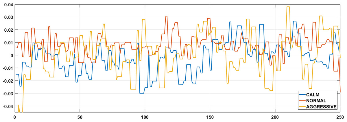
Figure 3: Example X-axis gyroscope data for three different driving classes.
Magnetometer
The magnetometer measures the strength of the magnetic field surrounding the device and provides data in microtesla (µT) units across the X, Y, and Z axes. These values are normalized within the range of −128 to +128. The total magnetic field detected by the device is the vector sum of the Earth’s geomagnetic field and the local magnetic fields surrounding the device. The magnetometer can function as a digital compass, and when integrated with accelerometer and gyroscope data, it allows for the detection of the device’s real-time movement and directional deviations (Sağbaş & Ballı, 2015).
Global positioning system (GPS)
The Global Positioning System (GPS), developed by the US Department of Defense in the 1970s, is a passive satellite-based navigation system that provides location and time information worldwide under all weather conditions (El-Rabbany, 2002). Modern smart devices determine location primarily via the GPS sensor, but can also use wireless networks and base stations with lower accuracy when GPS is unavailable. GPS signals include parameters such as latitude (positive north, negative south), longitude (positive east, negative west), speed (instantaneous velocity, invalid if negative or unavailable), and altitude (height above sea level in meters) (Ballı, Sağbaş & Peker, 2019b).
Overpass API
The Overpass API is a database system developed to efficiently query and manage data from the OpenStreetMap (OSM) project (Ramm, 2008). It updates global OSM data with minimal delay (typically only a few minutes) allowing users to access this information via the web. One of the primary goals of OSM is to foster new and innovative uses of geographic data. However, certain user queries may be too complex or specialized for traditional APIs that are primarily designed for map creators and geographic information editors. These challenges led to the development of the Overpass API (Olbricht, 2012). The Overpass API is optimized for users who need to perform specific and often complex queries against OSM data. It allows users to efficiently access data for specialized analysis and data processing projects that extend beyond the capabilities of typical map creation. The API’s design ensures that users can handle unique data retrieval needs, making it a valuable tool for research, development, and other specialized applications involving geographic information (Sağbaş, 2024).
OBD-II and ELM327
On-board diagnostics (OBD) has been mandatory in all light-duty vehicles since 1996, providing standardized monitoring of engine performance and emission control systems (Aris et al., 2007; Süzen & Kayaalp, 2018). Communication protocols are defined under ISO 15031 and SAE J1962, enabling external tools to access ECU data for diagnostics. OBD-II supports multiple protocols, including the CAN bus, allowing reliable collection of engine performance data essential for vehicle health monitoring (Kumar & Jain, 2022).
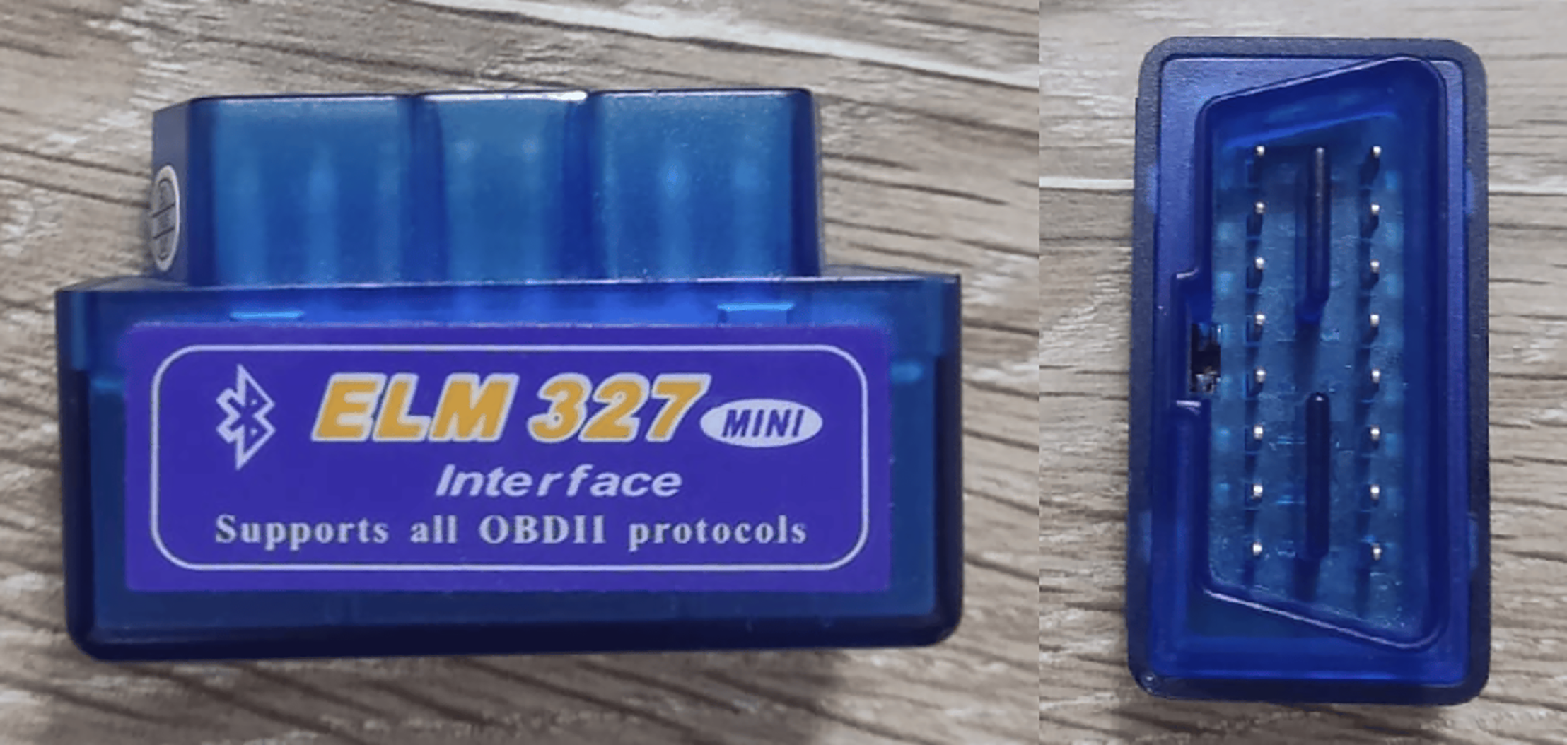
The ELM327 microcontroller, developed by ELM Electronics, facilitates communication between the OBD-II port and external devices by abstracting protocol complexity into a simple universal asynchronous receiver–transmitter (UART) interface. It supports universal serial bus (USB), Bluetooth, and wireless fidelity (Wi-Fi) connections, with wired USB offering greater reliability (Carignani et al., 2015). The multi-protocol device accommodates a wide range of OBD-II standards, such as SAE J1939, J1850 PWM, ISO 14230-4 KWP, ISO 15765-4 CAN, and ISO 9141-2 (Kumar & Jain, 2023). Through these protocols, parameters such as engine load, RPM, fuel system status, speed, coolant temperature, manifold pressure, airflow rate, and intake air temperature can be retrieved. In this study, the ELM327 device (Fig. 4) was employed for real-time data visualization and recording.
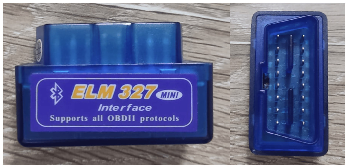
Figure 4: ELM327 device used in the study.
Android application and data logging setup
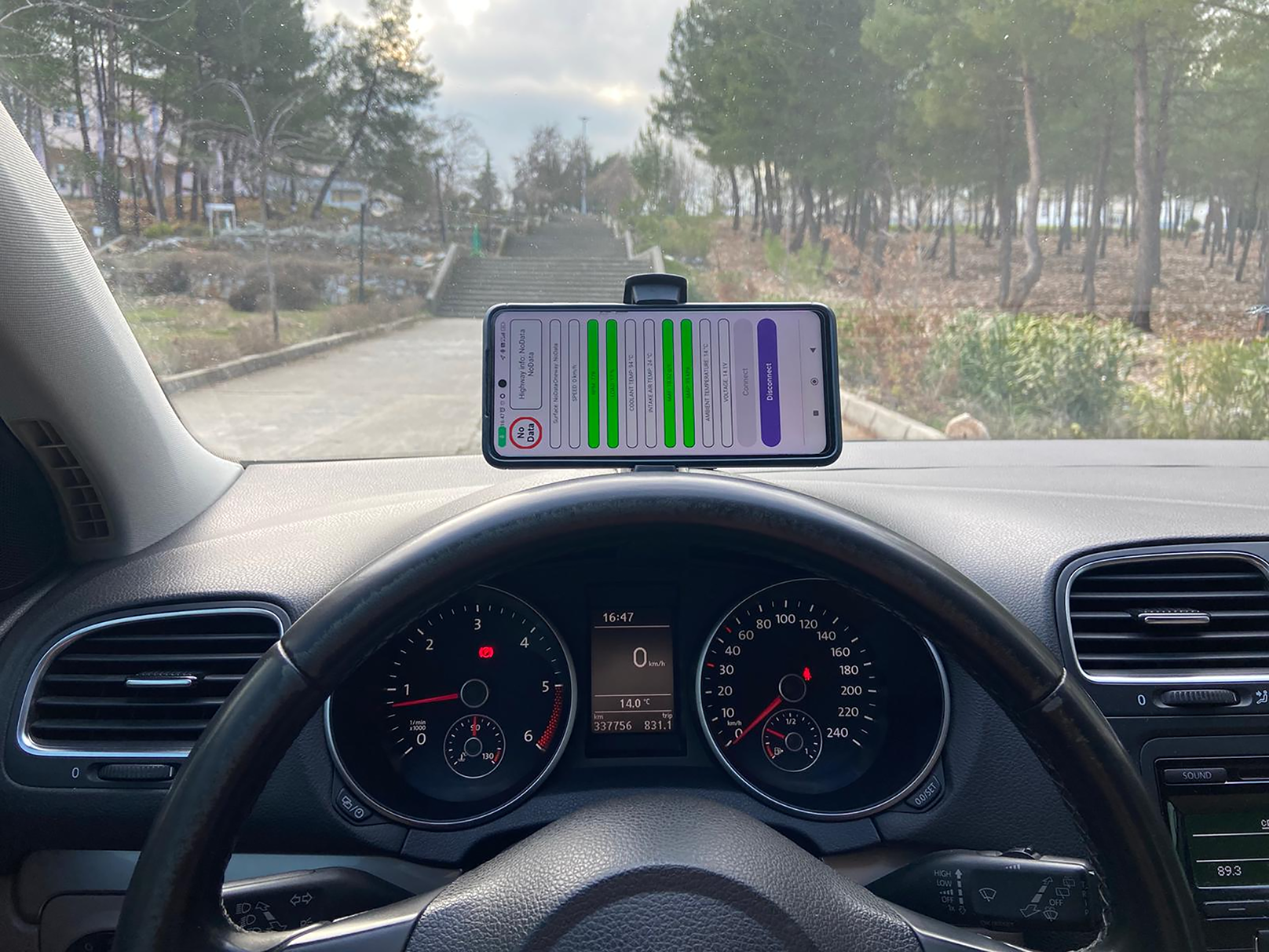
To classify driving behaviors, data regarding vehicle engine operations and various sensor data from the smartphone were collected. A specialized Android-based mobile application was developed to continuously and synchronously record this data. The primary goal of the application was to promote safe and economical driving practices. During the experiment, the smartphone was kept in a fixed position to ensure consistent data collection (Fig. 5).
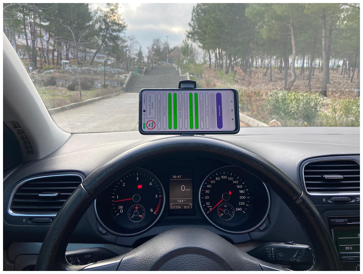
Figure 5: Position of the smartphone during the data acquisition phase.
The developed application utilizes the ELM327 adapter via the OBD-II port to obtain engine operation data from the vehicle. The data retrieved from the ECU is updated once per second. Table 1 presents the engine parameters, related parameter ID (PID) codes, and units used in this study.
| PID (hex) | Description | Units |
|---|---|---|
| x04 | Engine load value | % |
| x05 | Engine temperature | °C |
| x0B | Manifold absolute pressure | kPa |
| x0C | Engine RPM | RPM |
| x0D | Vehicle speed | km/h |
| x0F | Intake air temp | °C |
| x10 | Mass air flow rate | g/s |
| x46 | Ambient temperature | °C |
| ATRV | Voltage | V |
In addition, raw data obtained from the three-axis accelerometer, gyroscope, linear acceleration sensor, gravity sensor, and magnetometer were processed to analyze the dynamic movements and posture of the vehicle. The data sampling rate of the motion sensors was configured to provide 50 data points per second, ensuring high temporal resolution for capturing detailed motion and orientation changes during the driving process.
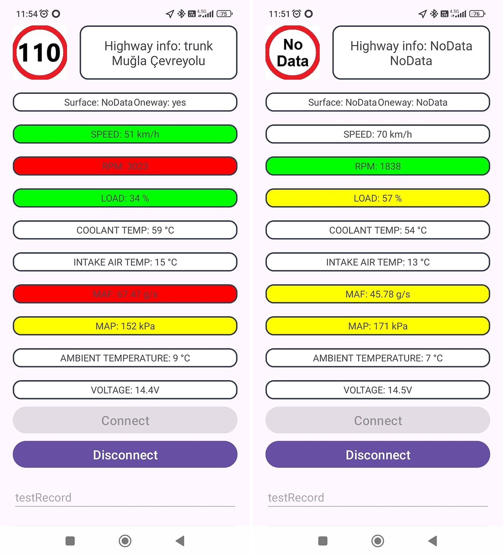
In addition to the data obtained from the ECU and motion sensors, latitude, longitude, altitude, and speed data were recorded from the GPS sensor to determine the location information of the vehicle and provide detailed information about the road conditions. The GPS data was integrated with the Overpass API and enriched with essential information such as the type of road the vehicle is on, legal speed limits, number of lanes, whether it is one-way, road surface type, and whether it requires tolls. This enriched data was used to create a warning system within the developed mobile application, offering real-time feedback to the driver and promoting safe driving practices. Screenshots of the developed application are shown in Fig. 6.
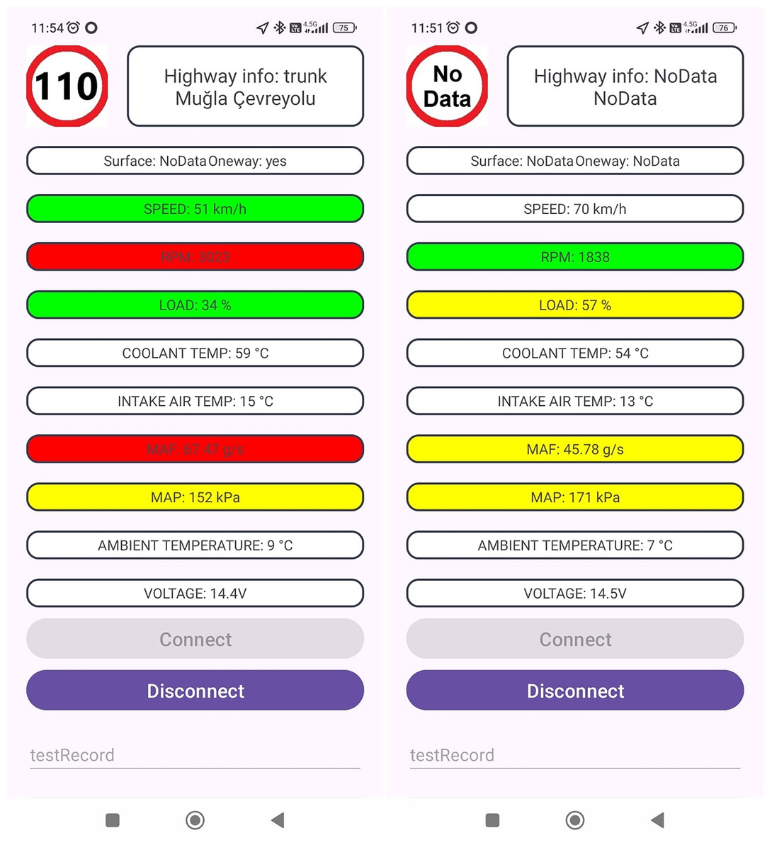
Figure 6: Engine operation data obtained for two different uses and visualization by the application.
Finally, as an additional factor to enhance the accuracy of the model, environmental audio data was collected. To prevent potential inconsistencies in the synchronization of textual and audio data, audio signals were not recorded in their raw form but rather by extracting specific features. These extracted features will be discussed in detail under the relevant analysis section. During the processing of the audio signals, a sampling frequency of 44.1 kHz was chosen, and the buffer size was set to 2,048.
The application provides the functionality to save the collected data in comma-separated values (CSV) format, with the file name being specified by the user (as shown in the last line of Fig. 6). These recorded data serve as a rich resource for analyzing the vehicle’s usage patterns and evaluating driving behaviors. The general flowchart outlining the data acquisition process for driving behavior classification is presented in Fig. 7.
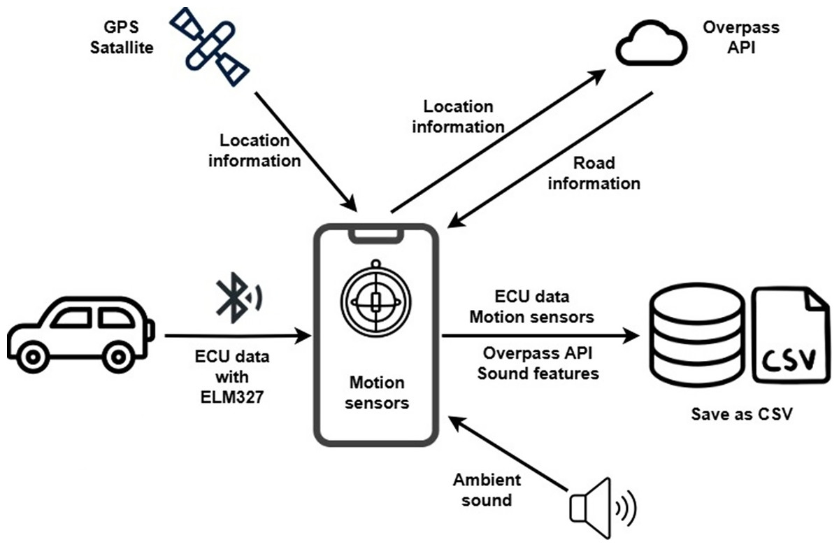
Figure 7: Data acquisition phase flowchart.
The developed mobile application can be utilized by individual drivers to receive real-time feedback on their driving habits, as well as by fleet managers to monitor driver performance and ensure compliance with safety standards. Additionally, the system’s ability to classify driving behaviors enables its integration into telematics-based insurance models, allowing insurance providers to assess driving risks more accurately and offer customized pricing based on real-time behavior.
To ensure transparency and reproducibility, the complete source code of the mobile application used for data acquisition is publicly available. DrivingHelper Application: Android-based application that collects real-time sensor data from vehicle ECU and smartphone sensors. Repository link: https://github.com/arifsagbas/DrivingHelper (https://doi.org/10.5281/zenodo.17286884).
Feature engineering and dataset preparation
To classify driving behaviors, data from engine operation and smartphone sensors were recorded using the data collection application described in ‘Android application and data logging setup’, and appropriate labeling was carried out. Driving behaviors were categorized into calm, normal, and aggressive in order to capture style-level differences that could be robustly inferred from the multimodal smartphone-centric signals. This coarse-grained design was adopted to maximize label reliability while avoiding conflation with cognitive states (e.g., distraction, drowsiness) that cannot be directly observed with the present sensor configuration. The calm class represents extremely cautious acceleration and deceleration behaviors, where the driver exhibits minimal fluctuations in speed. The normal class indicates a more dynamic driving style compared to the calm class, involving moderate accelerations and braking actions. The aggressive class is characterized by rapid accelerations and harsh braking, often observed in aggressive driving scenarios. In situations where the vehicle maintained a constant speed, classification was based on road conditions and engine speed. The data used in this study was collected from a Volkswagen Golf vehicle over a continuous driving period of approximately 2 h. The raw time-series data collected during driving sessions, segmented and labeled according to driving behavior classes is shared openly to promote replicability and further research. Raw dataset repository: https://github.com/arifsagbas/2025_obd_dataset (https://doi.org/10.5281/zenodo.17286874).
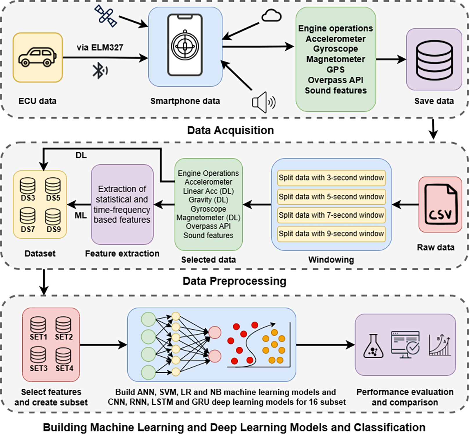
For subsequent analysis, the raw sensor data were segmented into overlapping time windows of 3, 5, 7, and 9 s, enabling the modeling of temporal driving patterns. These segments were saved in separate datasets named according to their respective window durations. The distribution of the driving behavior classes within the collected data is presented in Table 2.
| Window size | Dataset name | Class | #data |
|---|---|---|---|
| 3 s | DS3 | Calm | 1,239 |
| Normal | 574 | ||
| Aggressive | 855 | ||
| 5 s | DS5 | Calm | 744 |
| Normal | 344 | ||
| Aggressive | 513 | ||
| 7 s | DS7 | Calm | 530 |
| Normal | 246 | ||
| Aggressive | 367 | ||
| 9 s | DS9 | Calm | 413 |
| Normal | 190 | ||
| Aggressive | 286 |
In the classical machine learning pipeline, statistical and domain-relevant features were extracted from the segmented time windows to form structured input representations. These features were designed to capture temporal dynamics, signal variations, and contextual road information that are informative for behavior classification. Conversely, for deep learning models, no manual feature extraction was performed. Instead, the raw segmented sensor data, consisting of selected motion, engine, road metadata, and acoustic signal columns, were directly utilized as model inputs. These raw input matrices allowed deep architectures to learn hierarchical and latent representations automatically. Accordingly, separate data preprocessing pipelines were implemented to prepare the inputs for classical and deep learning methods, ensuring compatibility and methodological consistency throughout the study.
Classical feature extraction
Features extracted from motion sensors
Motion data were obtained from accelerometer and gyroscope sensors to analyze the vehicle’s dynamic movements and orientation. The magnetometer sensor was not included in this study. For each sensor (accelerometer and gyroscope), four features were extracted for each axis (X, Y, Z): mean, standard deviation, maximum value, and minimum value. This process resulted in a total of 24 motion-based features (four features × three axes × two sensors). These features capture the statistical characteristics of the vehicle’s motion along each axis, providing essential information about the vehicle’s behavior during driving.
Features extracted from ECU data
From engine-related parameters (engine speed, engine load, vehicle speed, MAF, and MAP), 22 statistical features were derived. These included minimum, maximum, average, and range values for each parameter, the rate of change of engine speed, delta load (change in engine load between successive measurements), and speed trend indicating acceleration or deceleration. Together, these features provide detailed insights into vehicle operating characteristics during driving.
Road information obtained from Overpass API
Beyond motion sensor and ECU features, five road-context attributes were derived from the Overpass API: the ratio of driver speed to the legal speed limit, highway category (e.g., trunk, secondary), surface type (e.g., asphalt, stabilized, dirt), one-way indicator, and number of lanes. These attributes provide environmental context that complements vehicle and driver dynamics, thereby enriching the classification of driving behaviors.
Features extracted from audio signals
Audio signals were incorporated as an additional modality to enhance driving behavior classification. Instead of storing raw audio, 13 statistical and spectral descriptors were computed, including root mean square (RMS), zero crossing rate, decibel level, amplitude, energy, dominant frequency, spectral centroid, spread, entropy, skewness, kurtosis, bandwidth, and rolloff. These features capture intensity, frequency distribution, and complexity of the auditory environment, providing complementary information beyond motion and ECU data.
Raw input configuration for deep learning
A total of 37 raw sensor columns were selected for deep learning models, without manual feature extraction, to provide a comprehensive view of vehicle dynamics, environmental context, and auditory feedback. These were grouped into four categories:
Motion sensors (15 columns): Tri-axial data from accelerometer, linear acceleration, gravity, gyroscope, and magnetometer, capturing fine-grained motion dynamics.
ECU data (five columns): Speed, engine load, RPM, mass air flow (MAF), and manifold absolute pressure (MAP), reflecting engine performance and driver interaction.
Road metadata (four columns): Attributes from the Overpass API (maxspeed, highway type, oneway status, and surface condition) providing environmental and infrastructural context.
Audio features (13 columns): Low-level descriptors (RMS, zero-crossing rate, spectral centroid, entropy, dominant frequency, etc.) derived from raw recordings, adding complementary auditory cues (e.g., tire or engine noise).
These 37 columns formed the unified raw input matrix for all deep learning models, allowing automatic learning of nonlinear temporal and contextual patterns across motion, mechanical, environmental, and auditory modalities.
Data normalization and encoding strategies
Prior to training classical machine learning models, a set of preprocessing steps was applied to the extracted feature dataset to ensure that all variables were represented in a format suitable for numerical algorithms. These operations included data type conversions, normalization of continuous features, and encoding of categorical variables. Firstly, all continuous attributes were normalized using z-score standardization to bring them to a common scale, thereby eliminating potential biases caused by varying units and magnitudes. This step was essential for ensuring the effectiveness and convergence of distance-based and gradient-based learning algorithms. For categorical data preprocessing, the speed trend, one-way, and lanes attributes (originally in categorical form) were transformed using label encoding, which maps each category to an integer value. The lanes feature was further transformed using one-hot encoding due to its limited and nominal nature, allowing the model to interpret each lane configuration as an independent binary feature. The highway type feature was encoded via frequency encoding, which replaces each category with its relative frequency in the dataset. This approach was chosen to preserve the global distributional information of road types while maintaining numerical compatibility. As a result of these transformations, the number of engineered features derived from Overpass API metadata increased from five to seven. This enriched representation aimed to enhance the descriptive power of the road environment context in the classification task. All transformations were applied globally across the full dataset to ensure consistency and were performed prior to model training in a reproducible preprocessing pipeline.
Unlike traditional machine learning methods that rely on handcrafted feature extraction, the deep learning models developed in this study utilize raw sensor data as direct input. However, in order to ensure model convergence and training stability, basic preprocessing steps were applied to the 37-column raw input matrix described in ‘Raw input configuration for deep learning’. These steps involved global normalization of continuous variables and label encoding of categorical features, preserving the raw temporal structure of each sample while standardizing input scales across the dataset. To this end, all CSV files corresponding to 3, 5, 7, and 9-s time windows were loaded from three behavior-specific folders (calm, normal, aggressive) and concatenated into a unified dataset. The dataset includes four categorical features, corresponding to road-related metadata extracted from the Overpass API: road type, oneway status, surface condition, and lane count. These categorical features were label-encoded using the LabelEncoder method, transforming each category into a unique integer value to ensure compatibility with embedding layers in deep learning architectures. The remaining 33 continuous features (originating from motion sensors, ECU parameters, and audio signals) were normalized using StandardScaler to yield zero-mean and unit-variance values across the entire dataset, a step critical for mitigating internal covariate shift and accelerating the training process. After encoding and normalization, the unified dataset was reshaped back into individual windowed samples and saved into behavior-specific folders, preserving the original time structure of each segment. No aggregation or manual feature engineering was applied at this stage, thereby allowing the deep learning models to autonomously learn hierarchical and temporal patterns directly from the preprocessed raw input. This standardized preprocessing approach was applied consistently across all time window configurations and driving behavior classes, ensuring methodological uniformity and reproducibility throughout the deep learning pipeline.
Classification models and experimental design
In this study, data collected from the ECU and smartphone sensors were used to analyze driving behaviors and categorize them into three distinct classes. To ensure a robust analysis, the raw data was divided into four separate datasets based on different time window lengths: 3, 5, 7, and 9 s. These window lengths provided varying temporal resolutions for capturing driving dynamics. For classical machine learning models, statistical and domain-specific features were extracted from each time window, resulting in an initial set of 64 features. After applying the preprocessing and encoding steps described in ‘Data normalization and encoding strategies’, the total number of features increased to 66. These labeled, feature-engineered windows constituted the input for classical machine learning algorithms. In parallel, deep learning models were trained on raw sensor data without any handcrafted feature extraction. Instead, each windowed segment was directly preserved as a matrix of size T × 37, where T represents the number of time steps per window. Each matrix contained raw measurements from motion sensors, ECU, road metadata, and audio features. This data representation enabled deep learning architectures to automatically extract hierarchical features and capture temporal dependencies from the raw, normalized sensor inputs. By preserving both engineered and raw data windows, the framework enabled a unified and systematic comparison across classical, deep learning, and transformer-based approaches in the context of driving behavior recognition.
When reviewing previous studies on the classification of driving behaviors, it becomes evident that deep learning methods have gained significant traction. For instance, studies by Zou et al. (2022), Lee & Yang (2023), Yen et al. (2021), Merenda et al. (2022), and Li, Lin & Chou (2022) widely employed deep learning techniques, such as convolutional neural networks and RNN, to analyze sensor data and classify driving behaviors. These methods are particularly suited for handling large and complex datasets, enabling the model to automatically extract relevant features and improve classification performance. On the other hand, traditional machine learning techniques also remain valuable in this field. Support vector machine, as seen in studies by Lattanzi & Freschi (2021), Kumar & Jain (2023), and Liu, Wang & Qiu (2020), are commonly used due to their effectiveness in dealing with high-dimensional data, especially when combined with kernel functions to handle non-linear relationships in driving behavior classification. Moreover, neural networks (Lattanzi & Freschi, 2021; Malik & Nandal, 2023), Markov models (Zou et al., 2022; Pirayre et al., 2022), and logistic regression (Liu, Wang & Qiu, 2020; Canal, Riffel & Gracioli, 2024) are also popular choices in the literature. These methods are especially useful for probabilistic modeling, sequential data analysis, and scenarios where interpretability of the results is important. Each of these methods offers distinct advantages, and their suitability depends on factors such as the size of the dataset, the complexity of the driving behaviors being analyzed, and the desired accuracy and interpretability of the model.
In line with the prevailing trends in the literature, where traditional machine learning approaches such as support vector machines (SVM), naïve Bayes (NB), logistic regression (LR), and artificial neural networks (ANN) continue to demonstrate effectiveness in behavior classification tasks, this study adopted a combination of both classical and deep learning-based models to evaluate and compare performance across various input representations. From the deep learning domain, convolutional neural networks (CNN), recurrent neural networks (RNN), long short-term memory (LSTM), and gated recurrent units (GRU) were selected due to their widespread adoption and proven capabilities in handling temporal and multivariate sensor data, particularly in the context of driving behavior analysis. All experiments were implemented in a Python environment using compute unified device architecture (CUDA)-enabled training on a system equipped with an NVIDIA RTX 4060 graphics processing unit (GPU), allowing for accelerated deep learning computations. Classical machine learning models were trained using the scikit-learn library, while deep learning models were built with PyTorch, ensuring flexible model customization and efficient batch-wise GPU utilization. For the SVM model, the kernel was set to “rbf” (radial basis function), with a regularization parameter C = 1.0 and kernel coefficient gamma = “scale”. The SVM classifier constructs a hyperplane that maximally separates classes in the feature space by solving an optimization problem (Eq. (1)), which aims to balance margin maximization and classification error using slack variables and kernel transformations.
(1) where is the feature mapping induced by the RBF kernel, is the penalty parameter, and are slack variables allowing for soft margin classification (Cortes & Vapnik, 1995). The logistic regression model used L2 regularization with the liblinear solver, and the regularization strength was set to . Logistic regression estimates the posterior probability of a class using the sigmoid function given in Eq. (2). The NB classifier employed the Gaussian variant with default variance smoothing. In this approach, the conditional likelihood is computed as shown in Eq. (3).
(2)
(3) assuming normality of the features (Rish, 2001). For the ANN baseline, a single hidden layer of 64 neurons was used with the rectified linear unit (ReLU) activation function, Adam optimizer, a learning rate of 0.001, and a maximum of 100 epochs with early stopping based on validation loss. ANNs perform layer-wise transformations of the input using affine mappings and non-linear activations. For a single-layer ANN, the output is defined as shown in Eq. (4).
(4) where is the weight matrix, is the bias vector, is the input, and is the activation function. This enables ANNs to model complex nonlinear relationships in the data (Bishop & Nasrabadi, 2006). In the deep learning experiments, all sequence-based models (RNN, LSTM, GRU) used a hidden size of 128, one recurrent layer, dropout rate of 0.3, and the Adam optimizer with a learning rate of 0.001. Mathematically, RNNs operate by updating the hidden state based on the current input and the previous hidden state , as expressed in Eq. (5).
(5)
However, due to the vanishing gradient problem in long sequences, LSTM and GRU architectures were introduced as solutions (Hochreiter & Schmidhuber, 1997; Chung et al., 2014). LSTMs use gating mechanisms to retain or forget information over time, with key operations defined by input, forget, and output gates. Similarly, GRUs simplify this structure by combining the forget and input gates into an update gate, improving computational efficiency while maintaining long-term dependency modeling. The CNN model consisted of two 1D convolutional layers (with 32 and 64 filters, kernel size 3), followed by global average pooling and a dense output layer with softmax activation. The core convolution operation in CNNs for time-series data can be described as shown in Eq. (6).
(6) where is the input signal, represents the convolutional filter weights, is the bias term, and indicates the layer index (LeCun et al., 2002). By stacking multiple convolutional layers and applying non-linear activations, CNNs automatically learn hierarchical feature representations from raw sensor input. Batch size was fixed at 64, and training was performed over 50 epochs with early stopping enabled (patience = 7 epochs).
In addition to the classical and deep learning models described above, this study also explored the PatchTST architecture (Nie et al., 2022), a recent transformer-based model tailored for time-series analysis. PatchTST utilizes a patch-wise representation strategy that segments the input sequence into non-overlapping temporal chunks, enabling the model to efficiently learn long-range dependencies without the recurrence bottleneck. This patching mechanism, combined with multi-head self-attention, allows for both local and global temporal feature extraction, making it particularly suitable for complex multivariate sensor streams such as those encountered in driving behavior classification. The foundation of PatchTST lies in the transformer architecture introduced by Vaswani et al. (2017), which replaces recurrence with a self-attention mechanism that computes contextualized embeddings by weighing interactions between all-time steps in parallel. This model incorporates learnable positional encodings (Gehring et al., 2017) and a classification token akin to bidirectional encoder representations from transformers (BERT) (Devlin et al., 2019), enabling it to summarize global sequence information. The attention mechanism used in PatchTST captures the relationships between different temporal segments (patches), making it more scalable and effective than traditional RNNs or CNNs when modeling long sequences (Zerveas et al., 2021; Wu et al., 2021).
In this study, the PatchTST model was implemented using variable architectural settings to systematically evaluate its performance across configurations. Specifically, the latent dimension size (d_model) was tested with both 64 and 128, while the number of transformer encoder layers (num_layers) was varied between 2, 3, 4, and 5. Each input sequence of shape (with being the number of time steps and the number of channels) was partitioned into non-overlapping patches of length 15. These patches were flattened and projected via a linear patch embedding layer, followed by the addition of learnable positional encodings and a classification token. The resulting sequence was then passed through a stack of multi-head self-attention layers with n_heads = 4 and a dropout rate of 0.2. The classification token output was finally normalized and mapped to class probabilities through a multi-layer perceptron (MLP) head with a LayerNorm and fully connected output layer. All PatchTST configurations employed the Adam optimizer (learning rate = 0.001, batch size = 64), and training was terminated through early stopping when the validation loss ceased to improve.
All models were evaluated using 10-fold cross-validation to ensure robust performance estimation. The primary evaluation metric was classification accuracy (Eq. (7)), and additional metrics such as precision, recall, and F1-score (Eqs. (8)–(10)) were computed to capture different aspects of classification performance.
(7)
(8)
(9)
(10)
The study also examined the effect of varying time window lengths on classification performance, as well as the incremental contribution of additional sensor modalities beyond the ECU data namely, motion sensors, road metadata, and environmental audio signals. To systematically evaluate the impact of each modality, the four time-windowed datasets (3, 5, 7, 9 s) were further partitioned into four distinct subsets based on the type of features they included. These feature configurations were designed to incrementally incorporate additional modalities, thereby enabling an analysis of their individual and combined influence on model accuracy. Table 3 summarizes the structure of these subsets. The inclusion of each feature type in a given configuration is marked with a “✓”, while the corresponding number of features for machine learning models and input columns for deep learning models is also provided.
| Model name | ECU | Motion sensors | Overpass API | Audio signals | #feature for ML | #columns for DL |
|---|---|---|---|---|---|---|
| SET1 | ✓ | 22 | 5 | |||
| SET2 | ✓ | ✓ | 46 | 20 | ||
| SET3 | ✓ | ✓ | ✓ | 53 | 24 | |
| SET4 | ✓ | ✓ | ✓ | ✓ | 66 | 37 |
This experimental design enabled a comparative investigation of feature-level importance under both traditional and deep learning frameworks, shedding light on the role of multimodal data integration in driving behavior classification. The scheme summarizing the general flow of the study is presented in Fig. 8.
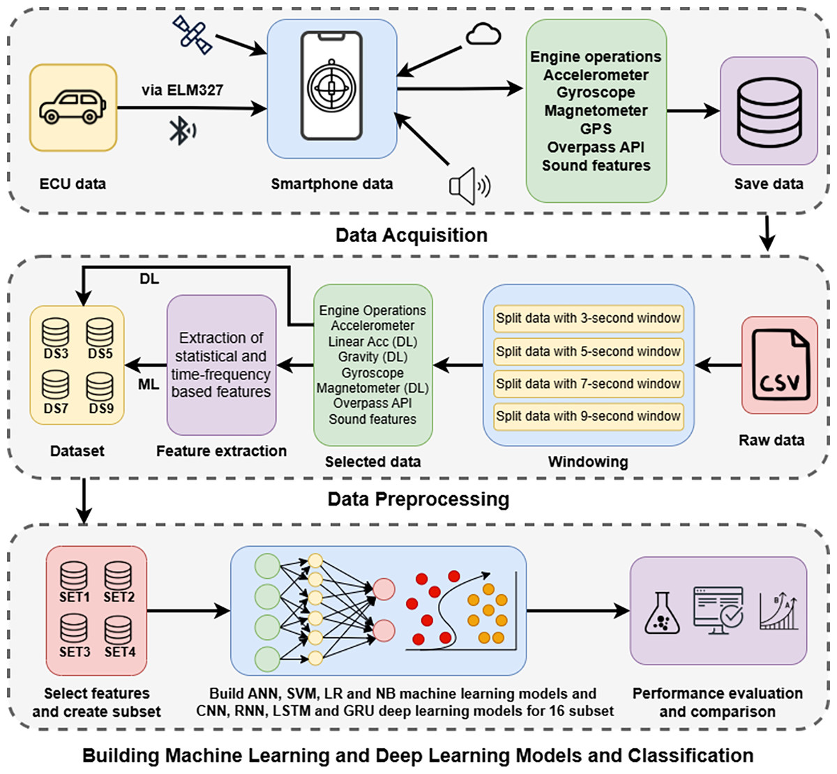
Figure 8: General flowchart of the study.
All machine learning and deep learning experiments, including data preprocessing, model training, evaluation metrics, and statistical testing, were implemented using Python. The full codebase is made publicly available to ensure reproducibility of the results. Experiment code repository: https://github.com/arifsagbas/comparison_ml_dl_patchtst_obd_data (https://doi.org/10.5281/zenodo.17286893).
Results and performance evaluation
Results from machine learning models
For classification, a set of commonly used and literature-backed classical machine learning models were employed: ANN, SVM, LR, and NB. All experiments were conducted in a Python-based environment using deterministic seeds and 10-fold cross-validation to ensure statistically reliable and reproducible performance estimates. Table 4 presents the classification results (accuracy, precision, recall, and F1-score) for each combination of dataset, feature subset, and classifier, illustrating temporal granularity and sensor modality affect performance.
| Dataset | Subset | Model | Accuracy | Precision | Recall | F1 | Model | Accuracy | Precision | Recall | F1 |
|---|---|---|---|---|---|---|---|---|---|---|---|
| DS3 | SET1 | ANN | 0.8722 | 0.8611 | 0.8539 | 0.8543 | NB | 0.8381 | 0.8210 | 0.8038 | 0.8102 |
| DS3 | SET2 | ANN | 0.8909 | 0.8761 | 0.8665 | 0.8701 | NB | 0.7406 | 0.7698 | 0.7692 | 0.7379 |
| DS3 | SET3 | ANN | 0.8913 | 0.8781 | 0.8655 | 0.8692 | NB | 0.6589 | 0.7520 | 0.7084 | 0.6664 |
| DS3 | SET4 | ANN | 0.9007 | 0.8883 | 0.8814 | 0.8834 | NB | 0.6548 | 0.7492 | 0.6977 | 0.6593 |
| DS5 | SET1 | ANN | 0.9063 | 0.8934 | 0.8900 | 0.8898 | NB | 0.8588 | 0.8407 | 0.8345 | 0.8363 |
| DS5 | SET2 | ANN | 0.9313 | 0.9230 | 0.9181 | 0.9193 | NB | 0.7820 | 0.8044 | 0.8115 | 0.7788 |
| DS5 | SET3 | ANN | 0.9369 | 0.9289 | 0.9270 | 0.9272 | NB | 0.7027 | 0.7776 | 0.7521 | 0.7089 |
| DS5 | SET4 | ANN | 0.9363 | 0.9279 | 0.9265 | 0.9261 | NB | 0.6939 | 0.7708 | 0.7367 | 0.6987 |
| DS7 | SET1 | ANN | 0.9020 | 0.8922 | 0.8850 | 0.8858 | NB | 0.8573 | 0.8421 | 0.8345 | 0.8358 |
| DS7 | SET2 | ANN | 0.9274 | 0.9200 | 0.9184 | 0.9173 | NB | 0.7769 | 0.7981 | 0.8101 | 0.7744 |
| DS7 | SET3 | ANN | 0.9387 | 0.9303 | 0.9292 | 0.9290 | NB | 0.7138 | 0.7736 | 0.7621 | 0.7187 |
| DS7 | SET4 | ANN | 0.9273 | 0.9185 | 0.9143 | 0.9155 | NB | 0.7068 | 0.7728 | 0.7475 | 0.7107 |
| DS9 | SET1 | ANN | 0.8920 | 0.8812 | 0.8729 | 0.8743 | NB | 0.8796 | 0.8637 | 0.8652 | 0.8635 |
| DS9 | SET2 | ANN | 0.9291 | 0.9231 | 0.9181 | 0.9184 | NB | 0.7975 | 0.8132 | 0.8270 | 0.7941 |
| DS9 | SET3 | ANN | 0.9256 | 0.9153 | 0.9142 | 0.9133 | NB | 0.7244 | 0.7786 | 0.7721 | 0.7274 |
| DS9 | SET4 | ANN | 0.9381 | 0.9314 | 0.9293 | 0.9293 | NB | 0.7334 | 0.7829 | 0.7722 | 0.7351 |
| DS3 | SET1 | LR | 0.8325 | 0.8155 | 0.7846 | 0.7925 | SVM | 0.8786 | 0.8705 | 0.8486 | 0.8567 |
| DS3 | SET2 | LR | 0.8520 | 0.8341 | 0.8098 | 0.8172 | SVM | 0.8846 | 0.8759 | 0.8517 | 0.8605 |
| DS3 | SET3 | LR | 0.8744 | 0.8595 | 0.8439 | 0.8496 | SVM | 0.8962 | 0.8888 | 0.8659 | 0.8744 |
| DS3 | SET4 | LR | 0.8842 | 0.8707 | 0.8568 | 0.8621 | SVM | 0.9037 | 0.8953 | 0.8795 | 0.8860 |
| DS5 | SET1 | LR | 0.8626 | 0.8468 | 0.8226 | 0.8297 | SVM | 0.9019 | 0.8952 | 0.8785 | 0.8846 |
| DS5 | SET2 | LR | 0.8782 | 0.8612 | 0.8446 | 0.8496 | SVM | 0.9063 | 0.8955 | 0.8837 | 0.8883 |
| DS5 | SET3 | LR | 0.9044 | 0.8920 | 0.8796 | 0.8839 | SVM | 0.9144 | 0.9048 | 0.8930 | 0.8977 |
| DS5 | SET4 | LR | 0.9132 | 0.9024 | 0.8920 | 0.8959 | SVM | 0.9144 | 0.9047 | 0.8946 | 0.8985 |
| DS7 | SET1 | LR | 0.8565 | 0.8463 | 0.8187 | 0.8246 | SVM | 0.8888 | 0.8831 | 0.8588 | 0.8662 |
| DS7 | SET2 | LR | 0.8845 | 0.8721 | 0.8539 | 0.8596 | SVM | 0.9002 | 0.8937 | 0.8716 | 0.8782 |
| DS7 | SET3 | LR | 0.9063 | 0.8973 | 0.8852 | 0.8885 | SVM | 0.9151 | 0.9124 | 0.8909 | 0.8980 |
| DS7 | SET4 | LR | 0.9098 | 0.9018 | 0.8887 | 0.8922 | SVM | 0.9151 | 0.9153 | 0.8911 | 0.8988 |
| DS9 | SET1 | LR | 0.8707 | 0.8596 | 0.8387 | 0.8455 | SVM | 0.9010 | 0.8956 | 0.8822 | 0.8865 |
| DS9 | SET2 | LR | 0.8875 | 0.8729 | 0.8593 | 0.8644 | SVM | 0.9078 | 0.8998 | 0.8871 | 0.8918 |
| DS9 | SET3 | LR | 0.9100 | 0.8992 | 0.8909 | 0.8939 | SVM | 0.9190 | 0.9134 | 0.9023 | 0.9063 |
| DS9 | SET4 | LR | 0.9111 | 0.9016 | 0.8911 | 0.8945 | SVM | 0.9269 | 0.9201 | 0.9143 | 0.9161 |
As shown in Table 4, richer feature subsets and longer time windows generally improve performance across most models. Moving from SET1 (ECU-only) to SET4 (including motion, Overpass, and audio data), a steady increase is observed in ANN, SVM, and LR metrics, whereas NB shows a slight decline due to its sensitivity to correlated and high-dimensional features. Longer windows (DS7, DS9) yield better results than shorter ones (DS3, DS5), as they capture more complete driving patterns and contextual transitions. ANN and SVM achieve the highest overall accuracies, benefiting from their ability to model non-linear relationships and adapt to higher feature dimensionality. In contrast, NB underperforms with complex inputs, while LR provides balanced but moderate accuracy with higher interpretability. The ranking across configurations remains consistent: ANN ≈ SVM > LR > NB. These findings confirm that multimodal sensor fusion and temporal context enhance classification performance, particularly for models capable of learning non-linear relationships. To provide a clearer understanding of how the models perform at the class level, confusion matrices corresponding to the best-performing configurations of each classifier are presented in Fig. 9.
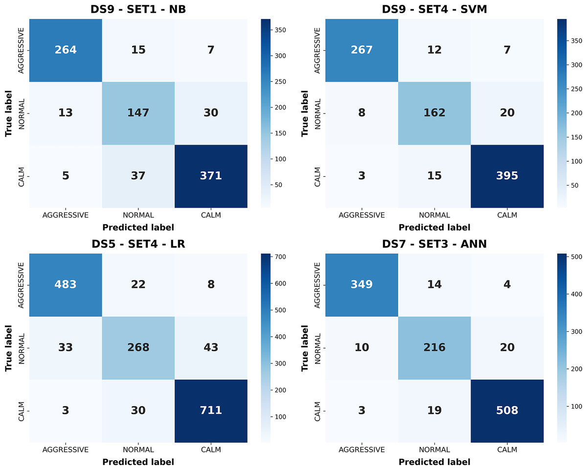
Figure 9: Confusion matrices of the best-performing configurations for each classical machine learning model.
Figure 9 illustrates the confusion matrices for the best configurations of each classifier, showing class-level prediction distributions. ANN (DS7–SET3) demonstrates the most balanced performance, effectively distinguishing calm and aggressive classes. SVM (DS9–SET4) also performs strongly but exhibits slightly higher confusion between normal and adjacent classes. LR achieves good accuracy but struggles in the normal class, while NB (DS9–SET1), limited to ECU data, fails to fully separate overlapping behaviors. Collectively, these results confirm that ANN offers the most reliable performance, followed by SVM; NB remains limited by feature simplicity. The receiver operating characteristic (ROC) curves corresponding to the best-performing configurations of these models are presented in Fig. 10, further illustrating their discriminative capabilities across the behavior classes.
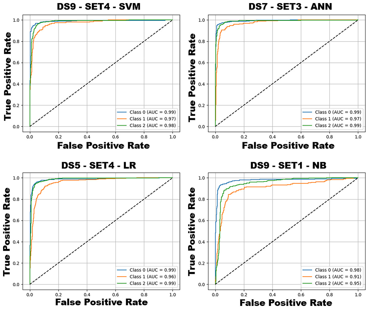
Figure 10: ROC curves and AUC scores of the best-performing configurations for each model.
Class 0: Aggressive, Class 1: Normal, Class 2: Calm.
Figure 10 shows the ROC curves of the best-performing configurations, illustrating class-wise discrimination. ANN (DS7–SET3) and SVM (DS9–SET4) achieve near-perfect separability (AUC ≈ 0.99 for aggressive and calm), while LR and NB perform slightly lower, particularly for the normal class. These results reaffirm that ANN and SVM provide the best overall discrimination, LR offers interpretable and moderate performance, and NB remains limited under simplified assumptions. The class-wise precision, recall, F1-score, and support values obtained from the best-performing configurations of each machine learning method are presented in Table 5.
| Method | Acc (%) | Precision | Recall | F1-score | Support | Dataset | Subset | |
|---|---|---|---|---|---|---|---|---|
| NB | 87.96% | Aggressive | 0.9362 | 0.9231 | 0.9296 | 286 | DS9 | SET1 |
| Normal | 0.7387 | 0.7737 | 0.7558 | 190 | ||||
| Calm | 0.9093 | 0.8983 | 0.9038 | 413 | ||||
| ANN | 93.88% | Aggressive | 0.9641 | 0.951 | 0.9575 | 367 | DS7 | SET3 |
| Normal | 0.8675 | 0.878 | 0.8727 | 246 | ||||
| Calm | 0.9549 | 0.9585 | 0.9567 | 530 | ||||
| SVM | 92.69% | Aggressive | 0.9604 | 0.9336 | 0.9468 | 286 | DS9 | SET4 |
| Normal | 0.8571 | 0.8526 | 0.8549 | 190 | ||||
| Calm | 0.936 | 0.9564 | 0.9461 | 413 | ||||
| LR | 91.32% | Aggressive | 0.9306 | 0.9415 | 0.936 | 513 | DS5 | SET4 |
| Normal | 0.8375 | 0.7791 | 0.8072 | 344 | ||||
| Calm | 0.9331 | 0.9556 | 0.9442 | 744 |
As noted, Table 5 presents only the best-performing configuration for each model. While this highlights the maximum potential of individual algorithms, direct cross-model comparisons are limited since the underlying dataset/subset combinations differ. ANN achieved the highest accuracy (93.88%) on DS7–SET3, showing balanced performance across all classes. SVM (DS9–SET4) followed closely with 92.69%, maintaining strong generalization. LR achieved 91.32%, while NB reached 87.96%, performing best in aggressive and calm classes but struggling with the normal class. Overall, ANN achieved the best class balance, SVM offered stable generalization, and LR provided interpretable reliability, whereas NB was most sensitive to class overlap.
Results from deep learning models
In addition to classical models, this study also explored the effectiveness of deep learning architectures on raw multivariate time-series data. Instead of relying on handcrafted features, the models were trained directly on segmented sensor sequences with varying window sizes (DS3–DS9), each represented as a T × 37 matrix containing motion, ECU, road, and audio features. Based on their widespread popularity and proven success in time-series classification tasks, four deep learning models were selected for this study: CNN, RNN, LSTM, GRU. All models were implemented using the PyTorch with CUDA (RTX 4060) acceleration. Performance was evaluated using 10-fold cross-validation, with the primary metrics being accuracy, precision, recall, F1-score, and AUC. Training and validation accuracy/loss curves for the best-performing configurations of each model are presented in Fig. 11.
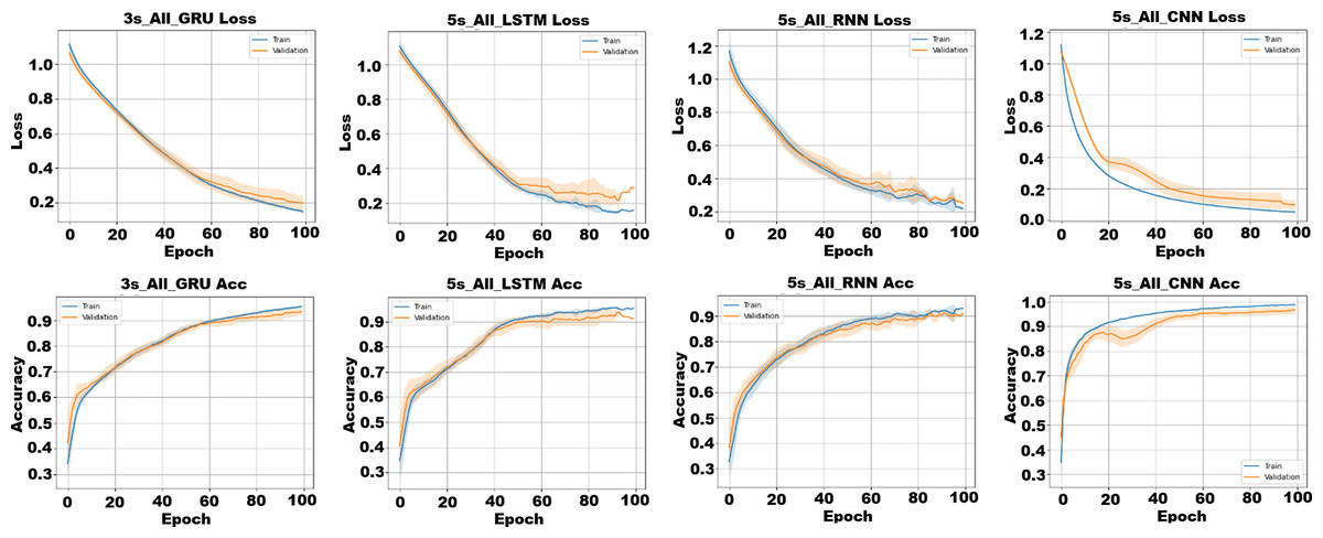
Figure 11: Training and validation accuracy/loss curves for the best-performing deep learning configurations on each model.
The term All indicates the use of the SET4 subset.
As shown in Fig. 11, all models converge effectively within 100 epochs under the full feature set (SET4). CNN and GRU exhibit the most stable and smooth convergence, with minimal overfitting and steady validation improvements. LSTM also performs strongly but shows mild overfitting after later epochs, while RNN converges more slowly and displays slightly noisier training curves, indicating limited robustness to temporal variations. Overall, CNN and GRU demonstrate the highest stability and generalization capacity under multimodal input. Table 6 presents the classification results for each combination of dataset, feature subset, and deep learning classifier.
| Dataset | Subset | Model | Accuracy | Precision | Recall | F1 | Model | Accuracy | Precision | Recall | F1 |
|---|---|---|---|---|---|---|---|---|---|---|---|
| DS3 | SET1 | CNN | 0.8632 | 0.8488 | 0.8338 | 0.8395 | LSTM | 0.8035 | 0.7930 | 0.7478 | 0.7592 |
| DS3 | SET2 | CNN | 0.9512 | 0.9458 | 0.9405 | 0.9427 | LSTM | 0.8947 | 0.8814 | 0.8772 | 0.8773 |
| DS3 | SET3 | CNN | 0.9580 | 0.9525 | 0.9516 | 0.9510 | LSTM | 0.8893 | 0.8753 | 0.8723 | 0.8701 |
| DS3 | SET4 | CNN | 0.9140 | 0.9038 | 0.9027 | 0.8994 | LSTM | 0.9029 | 0.8944 | 0.8799 | 0.8843 |
| DS5 | SET1 | CNN | 0.8838 | 0.8723 | 0.8587 | 0.8638 | LSTM | 0.8001 | 0.8036 | 0.7322 | 0.7361 |
| DS5 | SET2 | CNN | 0.9506 | 0.9443 | 0.9406 | 0.9420 | LSTM | 0.8776 | 0.8613 | 0.8543 | 0.8564 |
| DS5 | SET3 | CNN | 0.9594 | 0.9566 | 0.9482 | 0.9519 | LSTM | 0.8907 | 0.8774 | 0.8683 | 0.8705 |
| DS5 | SET4 | CNN | 0.9650 | 0.9620 | 0.9556 | 0.9583 | LSTM | 0.9107 | 0.9036 | 0.8901 | 0.8953 |
| DS7 | SET1 | CNN | 0.8862 | 0.8760 | 0.8628 | 0.8666 | LSTM | 0.8074 | 0.7918 | 0.7594 | 0.7680 |
| DS7 | SET2 | CNN | 0.9562 | 0.9533 | 0.9478 | 0.9491 | LSTM | 0.8634 | 0.8507 | 0.8417 | 0.8425 |
| DS7 | SET3 | CNN | 0.9624 | 0.9605 | 0.9528 | 0.9550 | LSTM | 0.8590 | 0.8448 | 0.8491 | 0.8435 |
| DS7 | SET4 | CNN | 0.9588 | 0.9546 | 0.9495 | 0.9505 | LSTM | 0.8905 | 0.8812 | 0.8681 | 0.8722 |
| DS9 | SET1 | CNN | 0.8879 | 0.8760 | 0.8671 | 0.8693 | LSTM | 0.7933 | 0.8027 | 0.7208 | 0.7208 |
| DS9 | SET2 | CNN | 0.9644 | 0.9608 | 0.9568 | 0.9580 | LSTM | 0.8612 | 0.8503 | 0.8293 | 0.8337 |
| DS9 | SET3 | CNN | 0.9629 | 0.9610 | 0.9575 | 0.9570 | LSTM | 0.8856 | 0.8730 | 0.8662 | 0.8669 |
| DS9 | SET4 | CNN | 0.9617 | 0.9591 | 0.9537 | 0.9548 | LSTM | 0.8806 | 0.8704 | 0.8585 | 0.8611 |
| DS3 | SET1 | GRU | 0.8159 | 0.8119 | 0.7626 | 0.7763 | RNN | 0.7862 | 0.7947 | 0.7200 | 0.7150 |
| DS3 | SET2 | GRU | 0.8890 | 0.8769 | 0.8634 | 0.8688 | RNN | 0.8414 | 0.8329 | 0.7950 | 0.8062 |
| DS3 | SET3 | GRU | 0.9212 | 0.9103 | 0.9092 | 0.9090 | RNN | 0.8759 | 0.8672 | 0.8657 | 0.8605 |
| DS3 | SET4 | GRU | 0.9284 | 0.9218 | 0.9117 | 0.9154 | RNN | 0.8766 | 0.8686 | 0.8521 | 0.8555 |
| DS5 | SET1 | GRU | 0.8151 | 0.8250 | 0.7488 | 0.7624 | RNN | 0.7889 | 0.7967 | 0.7124 | 0.7063 |
| DS5 | SET2 | GRU | 0.8875 | 0.8788 | 0.8576 | 0.8654 | RNN | 0.8282 | 0.8163 | 0.7873 | 0.7958 |
| DS5 | SET3 | GRU | 0.9175 | 0.9074 | 0.9023 | 0.9029 | RNN | 0.8595 | 0.8477 | 0.8256 | 0.8317 |
| DS5 | SET4 | GRU | 0.9238 | 0.9183 | 0.9048 | 0.9098 | RNN | 0.8838 | 0.8811 | 0.8555 | 0.8633 |
| DS7 | SET1 | GRU | 0.8047 | 0.7932 | 0.7447 | 0.7545 | RNN | 0.7724 | 0.6967 | 0.6827 | 0.6523 |
| DS7 | SET2 | GRU | 0.8660 | 0.8574 | 0.8277 | 0.8382 | RNN | 0.8345 | 0.8039 | 0.7827 | 0.7855 |
| DS7 | SET3 | GRU | 0.9072 | 0.8937 | 0.8952 | 0.8925 | RNN | 0.8484 | 0.8329 | 0.8213 | 0.8248 |
| DS7 | SET4 | GRU | 0.9221 | 0.9139 | 0.9067 | 0.9080 | RNN | 0.8660 | 0.8559 | 0.8405 | 0.8450 |
| DS9 | SET1 | GRU | 0.7970 | 0.7880 | 0.7222 | 0.7238 | RNN | 0.7426 | 0.7076 | 0.6509 | 0.6343 |
| DS9 | SET2 | GRU | 0.8552 | 0.8421 | 0.8200 | 0.8251 | RNN | 0.8248 | 0.8107 | 0.7743 | 0.7840 |
| DS9 | SET3 | GRU | 0.8957 | 0.8891 | 0.8811 | 0.8789 | RNN | 0.8271 | 0.8122 | 0.7858 | 0.7910 |
| DS9 | SET4 | GRU | 0.8991 | 0.8901 | 0.8794 | 0.8816 | RNN | 0.8697 | 0.8592 | 0.8372 | 0.8436 |
As shown in Table 6, each of the four deep learning models was systematically evaluated under all dataset–subset combinations, yielding 64 results in total. This design ensures comparability across models under consistent experimental conditions. Among all models and configurations, CNN consistently achieves the highest performance, particularly in subsets SET2–SET4, confirming the advantage of multimodal fusion. For instance, CNN reaches 96.5% accuracy (F1 = 95.8%) on DS5–SET4, highlighting its strong pattern-learning ability. LSTM follows with slightly lower accuracy (91.1%), performing best on longer windows but showing underfitting in ECU-only configurations (SET1). GRU demonstrates performance comparable to LSTM and sometimes higher (e.g., 92.2% accuracy (F1 = 90.8%) on DS7–SET4) benefiting from efficient gating and generalization even with shorter input lengths. RNN achieves the lowest performance, particularly under limited features (e.g., DS9–SET1 F1 = 63.4%), but improves with richer inputs. Across all models, performance increases from SET1 to SET4 and with longer windows, confirming the benefits of multimodal integration and temporal richness. To provide a clearer understanding of how the models perform at the class level, confusion matrices corresponding to the best-performing configurations of each classifier are presented in Fig. 12.
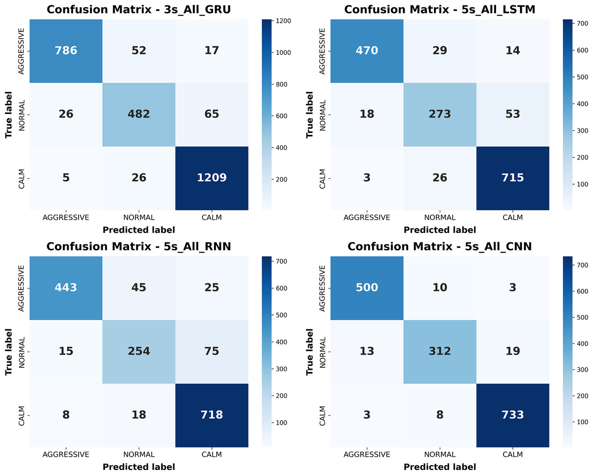
Figure 12: Confusion matrices of the best-performing configurations for each deep learning model.
As illustrated in Fig. 12, confusion matrices from the best-performing configurations of each deep learning model reveal distinct patterns in class-specific prediction behavior. CNN achieves the most balanced classification with minimal confusion across classes, followed closely by GRU. Both models effectively separate calm and aggressive behaviors, though normal class misclassifications persist across all networks. LSTM also performs well but shows moderate confusion in the normal class, while RNN exhibits the highest overall confusion, consistent with its difficulty in capturing long-term dependencies. Collectively, these results confirm that CNN and GRU deliver the most accurate and robust predictions, with CNN being the most consistent across all classes. The ROC curves corresponding to the best-performing configurations of these models are presented in Fig. 13, further illustrating their discriminative capabilities across the behavior classes.
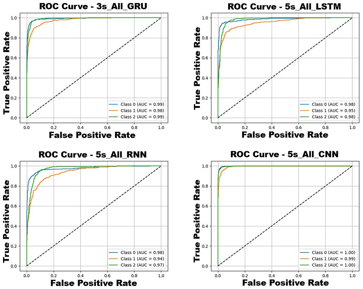
Figure 13: ROC curves and AUC scores of the best-performing configurations for each model.
Class 0: Aggressive, Class 1: Normal, Class 2: Calm.
As depicted in Fig. 13, the ROC curves and corresponding AUC scores validate these results. CNN achieves AUC = 1.00 for aggressive and calm, and 0.99 for normal, confirming near-perfect separability. GRU and LSTM follow closely (AUC ≈ 0.99–0.95), while RNN lags slightly, particularly for the normal class (AUC = 0.94). These findings reinforce that CNN and GRU provide the best class separability, while LSTM performs competitively and RNN remains the least effective under complex multimodal conditions. The class-wise precision, recall, F1-score, and support values obtained from the best-performing configurations of each method are presented in Table 7.
| Method | Acc (%) | Precision | Recall | F1-score | Support | Dataset | Subset | |
|---|---|---|---|---|---|---|---|---|
| CNN | 96.50% | Aggressive | 0.9690 | 0.9747 | 0.9718 | 513 | DS5 | SET4 |
| Normal | 0.9455 | 0.9070 | 0.9258 | 344 | ||||
| Calm | 0.9709 | 0.9852 | 0.9780 | 744 | ||||
| LSTM | 91.07% | Aggressive | 0.9572 | 0.9162 | 0.9363 | 513 | DS5 | SET4 |
| Normal | 0.8323 | 0.7936 | 0.8125 | 344 | ||||
| Calm | 0.9143 | 0.9610 | 0.9371 | 744 | ||||
| GRU | 92.84% | Aggressive | 0.9572 | 0.9162 | 0.9363 | 513 | DS3 | SET4 |
| Normal | 0.8323 | 0.7936 | 0.8125 | 344 | ||||
| Calm | 0.9143 | 0.9610 | 0.9371 | 744 | ||||
| RNN | 88.38% | Aggressive | 0.9506 | 0.8635 | 0.9050 | 513 | DS5 | SET4 |
| Normal | 0.8013 | 0.7384 | 0.7685 | 344 | ||||
| Calm | 0.8778 | 0.9651 | 0.9193 | 744 |
Table 7 summarizes the best configurations of each model. CNN (DS5–SET4) achieved the highest accuracy (96.5%), with outstanding F1-scores across all classes (0.97–0.98). GRU (DS3–SET4) followed with 92.8%, showing excellent efficiency even with shorter windows. LSTM reached 91.1%, performing strongly on calm and aggressive classes but weaker in normal. RNN achieved 88.4%, limited by its difficulty in learning long-term dependencies. Overall, CNN remains the top performer, while GRU offers a strong balance between performance and computational cost. LSTM maintains competitive accuracy, and RNN is the least suitable for complex temporal modeling.
Results from PatchTST models
To further investigate the performance of transformer-based models in driving behavior classification, a series of comprehensive experiments were conducted using the PatchTST architecture. Unlike traditional recurrent or convolutional models, PatchTST employs a patch-wise tokenization mechanism that enables efficient modeling of long-term temporal dependencies. Two latent dimensions (d_model = 64, 128) and four encoder depths (2–5 layers) were tested, producing eight model variants. Each variant was evaluated across four sensor configurations (SET1–SET4) and four window lengths (3, 5, 7, 9 s), resulting in 128 experiments. The results are summarized in Table 8, which outlines the performance trends across these configurations.
| dModel | 64 | 128 | |||||||
|---|---|---|---|---|---|---|---|---|---|
| #layer | 2 | 3 | 4 | 5 | 2 | 3 | 4 | 5 | |
| DS3 | SET1 | 87.63 | 87.15 | 85.38 | 84.11 | 86.06 | 84.78 | 83.77 | 77.62 |
| SET2 | 94.08 | 94.04 | 92.47 | 91.12 | 93.03 | 91.91 | 86.58 | 78.04 | |
| SET3 | 94.53 | 95.13 | 93.93 | 83.06 | 94.42 | 93.21 | 85.95 | 72.04 | |
| SET4 | 95.54 | 95.28 | 93.44 | 77.96 | 95.39 | 93.22 | 89.54 | 71.33 | |
| DS5 | SET1 | 89.19 | 88.82 | 88.14 | 85.14 | 88.26 | 86.95 | 86.01 | 84.64 |
| SET2 | 93.13 | 92.69 | 93.57 | 89.25 | 93.26 | 91.88 | 89.45 | 78.41 | |
| SET3 | 95.06 | 94.19 | 93.13 | 84.32 | 95.44 | 93.57 | 86.26 | 71.01 | |
| SET4 | 95.25 | 93.75 | 94.19 | 87.19 | 94.69 | 93.94 | 88.00 | 81.26 | |
| DS7 | SET1 | 89.24 | 89.15 | 88.27 | 87.58 | 89.23 | 88.01 | 87.40 | 85.56 |
| SET2 | 93.52 | 92.57 | 92.56 | 90.73 | 91.95 | 91.86 | 90.64 | 85.21 | |
| SET3 | 93.44 | 93.61 | 94.67 | 88.89 | 93.7 | 93.00 | 88.96 | 76.18 | |
| SET4 | 95.10 | 94.31 | 95.19 | 86.35 | 95.10 | 95.62 | 93.43 | 81.16 | |
| DS9 | SET1 | 91.00 | 90.55 | 90.33 | 90.89 | 90.10 | 90.66 | 88.86 | 87.17 |
| SET2 | 93.14 | 93.70 | 92.8 | 91.44 | 92.46 | 93.25 | 92.01 | 87.07 | |
| SET3 | 95.16 | 95.39 | 94.26 | 85.93 | 93.44 | 93.70 | 88.19 | 79.87 | |
| SET4 | 96.29 | 95.50 | 95.50 | 86.83 | 96.06 | 95.28 | 93.25 | 83.91 | |
Table 8 shows that models with lower dimensionality (d_model = 64) and fewer encoder layers (2–3) consistently outperform deeper, higher-capacity variants. Deeper models with d_model = 128 often show reduced accuracy due to overfitting or instability. Performance improves with richer sensor inputs (particularly SET4, which yields the best results across all datasets) and with longer time windows (DS7, DS9), which provide broader temporal context. The best accuracy (96.29%) was achieved on DS9 using d_model = 64, 2 layers, and SET4, indicating that compact transformer architectures can deliver state-of-the-art accuracy with efficient computation. These results highlight the importance of architectural simplicity and multimodal richness in optimizing transformer-based time-series classification. In continuation of the analysis, Table 9 presents the detailed class-wise performance metrics (precision, recall, F1-score and support) corresponding to the highest-performing PatchTST configuration identified for each dataset, as reported in Table 8.
| Dataset | Subset | dModel | #layer | Accuracy | Precision | Recall | F1-score | Support | |
|---|---|---|---|---|---|---|---|---|---|
| DS3 | SET4 | 64 | 2 | 95.54% | Aggresive | 0.9757 | 0.9650 | 0.9700 | 85.50 |
| Calm | 0.9613 | 0.9726 | 0.9667 | 124.0 | |||||
| Normal | 0.9141 | 0.9042 | 0.9087 | 57.30 | |||||
| DS5 | SET3 | 128 | 2 | 95.44% | Aggresive | 0.9771 | 0.9707 | 0.9735 | 51.30 |
| Calm | 0.9633 | 0.9704 | 0.9665 | 74.40 | |||||
| Normal | 0.9033 | 0.8951 | 0.8988 | 34.40 | |||||
| DS7 | SET4 | 128 | 3 | 95.62% | Aggresive | 0.9893 | 0.9538 | 0.9706 | 36.60 |
| Calm | 0.9555 | 0.9849 | 0.9696 | 53.10 | |||||
| Normal | 0.9195 | 0.8980 | 0.9046 | 24.50 | |||||
| DS9 | SET4 | 64 | 2 | 96.29% | Aggresive | 0.9899 | 0.9791 | 0.9841 | 28.50 |
| Calm | 0.9519 | 0.983 | 0.9668 | 41.30 | |||||
| Normal | 0.9546 | 0.8947 | 0.9200 | 19.10 |
Table 9 provides class-wise metrics for the top-performing configuration in each dataset. Across all cases, PatchTST achieves high and balanced F1-scores, particularly for aggressive and calm behaviors. For example, on DS9, the best model (d_model = 64, 2 layers, SET4) achieves 96.29% accuracy with F1-scores above 0.96 in both classes. The normal class performs slightly lower due to its transitional nature, but overall class balance remains strong. These findings confirm that a properly tuned PatchTST model can generalize robustly across diverse driving behaviors. To support and further illustrate the quantitative results presented above, Fig. 14 provides the training and validation accuracy and loss curves for each dataset based on the corresponding best-performing PatchTST configuration.
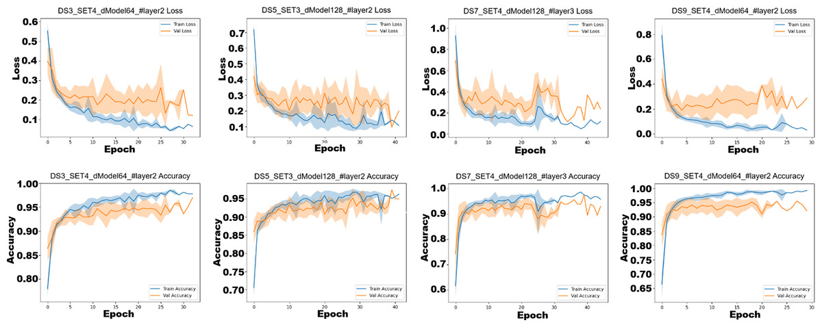
Figure 14: Training and validation loss and accuracy curves for the best-performing PatchTST configurations on each dataset.
Figure 14 shows training and validation curves of the best configurations. All models converge rapidly within the first few epochs, maintaining close alignment between training and validation losses. Minor fluctuations in DS7 and DS5 suggest slight instability in deeper models, but no evidence of severe overfitting is observed. In DS9 (SET4, d_model = 64, 2 layers), both training and validation accuracies exceed 95%, indicating excellent convergence and generalization. Overall, compact PatchTST models exhibit stable optimization and strong learning dynamics across datasets. To further analyze the model’s class-wise predictive performance, the confusion matrices of the best-performing configurations for each dataset are presented in Fig. 15.
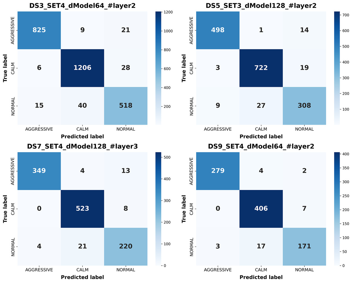
Figure 15: Confusion matrices of the best-performing PatchTST configurations for each dataset.
The confusion matrices in Fig. 15 confirm the model’s consistent and balanced performance. Aggressive and calm behaviors are almost perfectly classified, with minor overlap in the normal class across datasets. DS3 and DS5 maintain strong diagonal dominance, while DS7 shows slightly more confusion due to transitional patterns. These results reinforce the PatchTST’s capacity to distinguish between distinct behaviors, particularly at the extremes. Figure 16 presents the ROC curves corresponding to the best-performing configurations for each dataset.
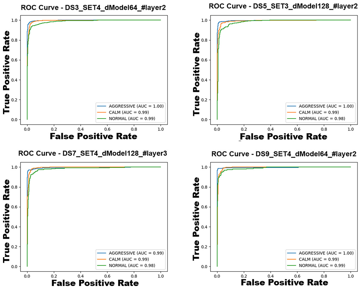
Figure 16: ROC curves and AUC values for the best PatchTST configurations across datasets DS3–DS9.
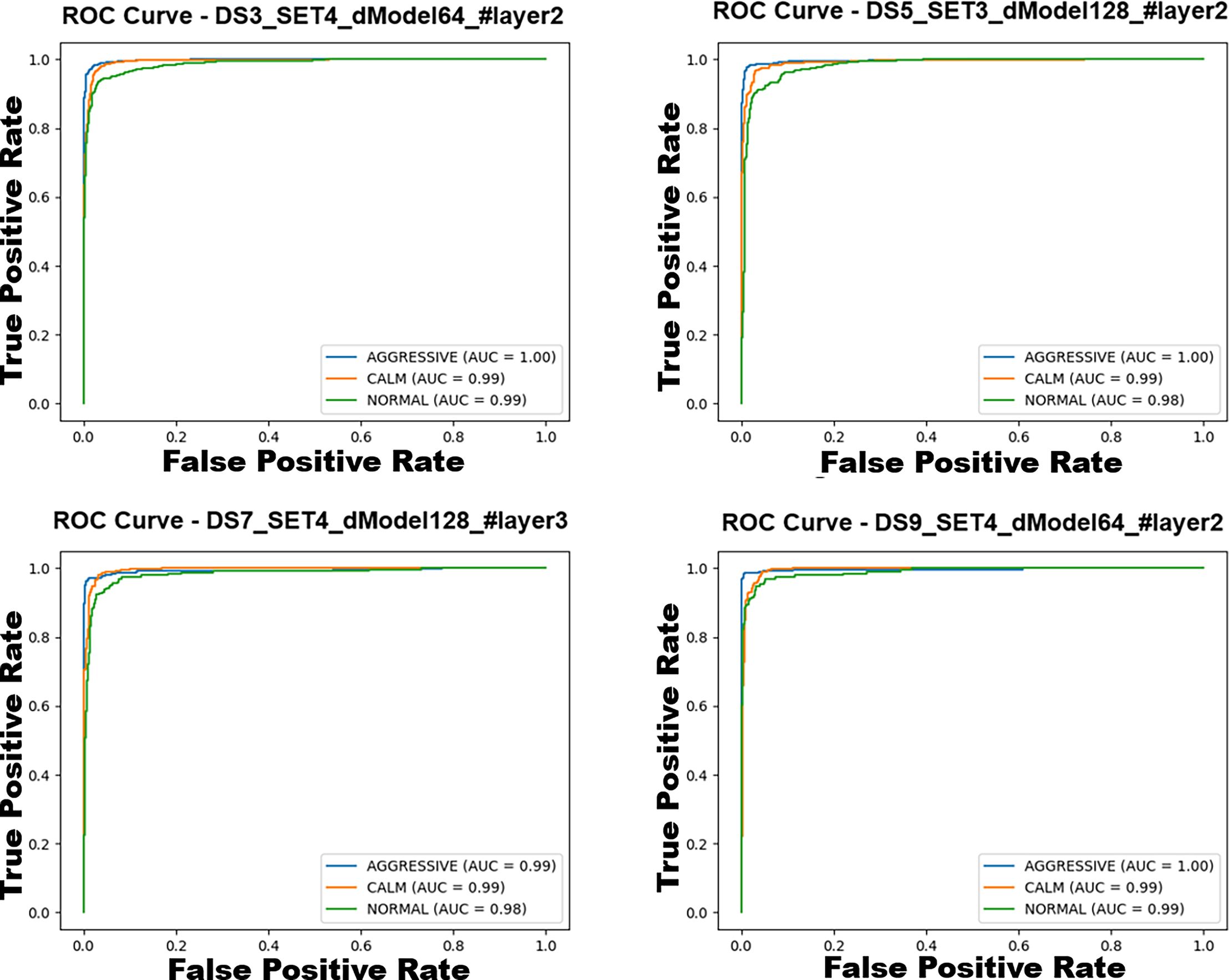
In Fig. 16, all AUC values exceed 0.98, indicating excellent separability across the three classes. In particular, DS9 and DS3 achieve near-perfect AUC scores of 1.00 for the aggressive class and 0.99 for calm and normal classes. The slightly lower but still impressive AUC values observed in DS5 and DS7 further validate the model’s robustness, even in configurations with higher dimensional complexity. These results align with the precision, recall, F1 metrics and confusion matrix analyses, reinforcing the model’s generalization capacity and consistent high performance across diverse sensor and temporal settings.
Discussion
Performance evaluation of the proposed method
The experimental results reveal several important insights regarding the classification performance of both classical machine learning and deep learning models in the context of driving behavior recognition. Among classical models, ANN demonstrated the most consistent and superior performance across different datasets and feature subsets, achieving its highest accuracy of 93.88% on DS7 with SET3. SVM closely followed, with particularly stable results and a peak accuracy of 92.69% on DS9 with SET4. LR also performed competitively, especially when rich multimodal inputs were provided, reaching 91.32% accuracy on DS5 with SET4. In contrast, NB showed diminished performance with more complex feature sets, likely due to its assumption of conditional independence among features, but still achieved a strong result of 87.96% on DS9 with SET1.
When PatchTST experiments are evaluated in this context, further statistical analyses were conducted to investigate how architectural design choices and data configurations influence classification performance. A multifactorial analysis of variance (ANOVA) was applied to four categorical factors (dModel, layer, dataset, and subset) to determine their individual contributions to the observed accuracy scores. As shown in Table 10, all four variables yielded statistically significant p-values (p < 0.0001), confirming that both architectural depth and input diversity considerably impact model performance.
| Source | Sum of squares | Degrees of freedom | F-value | p-value |
|---|---|---|---|---|
| dModel | 312.56 | 1 | 21.55 | <0.0001 |
| Layer | 1,272.35 | 3 | 29.28 | <0.0001 |
| Dataset | 540.42 | 3 | 12.44 | <0.0001 |
| Subset | 478.79 | 3 | 11.02 | <0.0001 |
| Residual | 5,277.27 | 117 |
According to the ANOVA results, layer count was identified as the most influential factor, followed by dataset, subset, and dModel. To gain deeper insight into pairwise differences among group levels, Tukey’s Honest Significant Difference (HSD) test was applied. The post-hoc analysis of the subset factor, as presented in Table 11, revealed statistically significant improvements in accuracy between SET1 and both SET2 and SET4, demonstrating that incorporating richer sensor modalities notably enhances performance.
| Group 1 | Group 2 | Mean diff | p-adj | Lower | Upper | Significant |
|---|---|---|---|---|---|---|
| SET1 | SET2 | 3.44 | 0.0457 | 0.05 | 6.84 | Yes |
| SET1 | SET3 | 2.37 | 0.2685 | −1.02 | 5.77 | No |
| SET1 | SET4 | 3.79 | 0.0224 | 0.39 | 7.18 | Yes |
| SET2 | SET3 | −1.07 | 0.8454 | −4.46 | 2.33 | No |
| SET2 | SET4 | 0.34 | 0.9935 | −3.05 | 3.74 | No |
Regarding the dModel parameter, Table 12 shows that models using a lower latent dimension (dModel = 64) significantly outperformed those with dModel = 128, suggesting better generalization capacity and reduced risk of overfitting.
| Group 1 | Group 2 | Mean diff | p-adj | Lower | Upper | Significant |
|---|---|---|---|---|---|---|
| 64 | 128 | 2.24 | 0.0003 | 1.08 | 3.40 | Yes |
For the layer factor, Table 13 highlights a consistent drop in performance as model depth increased, with two-layer architectures achieving significantly higher accuracy than deeper counterparts. This underscores the importance of architectural simplicity in temporal modeling tasks.
| Group 1 | Group 2 | Mean diff | p-adj | Lower | Upper | Significant |
|---|---|---|---|---|---|---|
| 2 | 3 | 0.80 | 0.0015 | 0.20 | 1.40 | Yes |
| 2 | 4 | 1.89 | 0.0001 | 1.28 | 2.50 | Yes |
| 2 | 5 | 3.07 | 0.0001 | 2.47 | 3.67 | Yes |
| 3 | 4 | 1.09 | 0.0001 | 0.49 | 1.69 | Yes |
| 3 | 5 | 2.27 | 0.0001 | 1.67 | 2.87 | Yes |
| 4 | 5 | 1.18 | 0.0001 | 0.58 | 1.78 | Yes |
Finally, in terms of dataset, Table 14 shows that DS9 consistently outperformed other datasets, indicating that longer time windows provide more informative temporal context and contribute positively to classification accuracy.
| Group 1 | Group 2 | Mean diff | p-adj | Lower | Upper | Significant |
|---|---|---|---|---|---|---|
| DS3 | DS5 | −0.34 | 0.9043 | −2.74 | 2.06 | No |
| DS3 | DS7 | −1.45 | 0.0948 | −3.85 | 0.95 | No |
| DS3 | DS9 | −3.53 | 0.0003 | −5.93 | −1.13 | Yes |
| DS5 | DS7 | −1.10 | 0.2148 | −3.50 | 1.30 | No |
| DS5 | DS9 | −3.19 | 0.0010 | −5.59 | −0.79 | Yes |
| DS7 | DS9 | −2.09 | 0.0249 | −4.49 | −0.31 | Yes |
These findings collectively emphasize that careful tuning of architectural complexity (particularly limiting layer depth and dimensionality), combined with the strategic selection of feature subsets and temporal granularity, is critical to optimizing transformer-based models such as PatchTST for driving behavior recognition.
On the deep learning side, CNN outperformed all other models, achieving the highest overall classification accuracy of 96.50% on DS5 with SET4. This demonstrates the effectiveness of CNNs in learning discriminative spatial-temporal features from multivariate sensor sequences. Recurrent architectures, particularly GRU and LSTM, also yielded competitive results, with GRU achieving 92.84% accuracy on DS3 with SET4 and LSTM reaching 91.07% on DS5 with SET4. RNNs, while trailing slightly in overall accuracy, performed reasonably well in scenarios with shorter time windows or less complex input features. Overall, the results show that increasing the temporal resolution (i.e., using longer time windows such as in DS5 or DS9) and integrating multimodal sensor data (e.g., motion, overpass metadata, and sound in SET4) substantially improve classification performance. The combination of deep learning methods and rich input representations leads to more robust models capable of capturing the dynamic patterns underlying aggressive, normal, and calm driving behaviors.
Normality tests (Shapiro–Wilk) indicated that both machine learning (ML) and deep learning (DL) accuracy scores violated the assumption of normality (p < 0.0001). Therefore, the Mann–Whitney U test was used to compare the two approaches. The results showed no statistically significant difference between ML and DL models in terms of classification accuracy (p = 0.4832), suggesting that both paradigms offer comparable performance in the context of driving behavior classification.
Since the normality assumption was violated for multiple feature subsets (e.g., SET4: p = 0.0107, SET3: p = 0.0005), a non-parametric Kruskal–Wallis H test was conducted to assess the effect of different feature sets on model performance. The test revealed statistically significant differences (H(4) = …, p < 0.0001). To identify the specific differences between groups, a Dunn’s post-hoc test with Bonferroni correction was performed. The results (see Table 15) indicate that the ECU-only configuration significantly underperformed compared to all other subsets (e.g., SET1 vs. SET4: p ≈ 1.6 × 10−36), whereas no significant difference was observed between the SET4 and SET3 subsets (p = 1.0000).
| SET 1 | SET 2 | SET 3 | SET 4 | Normalized | |
|---|---|---|---|---|---|
| SET 1 | 1 | 2.01E−17 | 1.39E−30 | 1.64E−36 | 7.44E−23 |
| SET 2 | 2.01E−17 | 1 | 0.033281 | 0.000528 | 1 |
| SET 3 | 1.39E−30 | 0.033281 | 1 | 1 | 2.37E−05 |
| SET 4 | 1.64E−36 | 0.000528 | 1 | 1 | 9.37E−09 |
| Normalized | 7.44E−23 | 1 | 2.37E−05 | 9.37E−09 | 1 |
To further examine the influence of both model architecture and feature subset on classification accuracy, a two-way ANOVA was conducted. As shown in Table 16 model type had a statistically significant main effect (F(19, 1,248) = 4.35, p = 0.0017), while the main effect of the feature subset and the interaction between model and subset were not significant (p = 1.0000 and p = 0.9576, respectively). This suggests that accuracy was primarily determined by the model architecture, regardless of the input feature set used.
| sum_sq | df | F | PRc (>F) | |
|---|---|---|---|---|
| C(model) | 0.108352 | 19 | 4.354195 | 0.001682 |
| C(subset) | −2.16E−15 | 4 | −4.12E−13 | 1 |
| C(model):C(subset) | 0.028961 | 76 | 0.290957 | 0.957644 |
| Residual | 1.634523 | 1,248 |
Comparison with studies in the literature
A direct comparison between the present study and other studies in the literature is not feasible due to significant differences in data sources and the devices employed. Generally, research on driver behavior classification categorizes driving styles into safe (Fadzil et al., 2026), unsafe (Lattanzi & Freschi, 2021; Mohammed et al., 2023), and aggressive (Singh & Singh, 2022; Ameen et al., 2021; Lin, Zhang & Chang, 2023; Merenda et al., 2022; Yarlagadda & Pawar, 2022; Zhang & Lin, 2021; Al-Rakhami et al., 2021) driving behaviors. Additionally, certain studies focus on enhancing driving economy (Azadani & Boukerche, 2022; Rastegar et al., 2024; Canal, Riffel & Gracioli, 2024; Yen et al., 2021; Pirayre et al., 2022) or vehicle ownership control (Martinelli et al., 2020).
The most commonly utilized data source for driver behavior classification is OBD-II data, which is typically collected using the ELM327 device (Kumar & Jain, 2023; Ameen et al., 2021; Fattahi, Golroo & Ghatee, 2023). However, alternative devices such as iSaddle (Singh & Singh, 2022), HH OBD Advanced (Merenda et al., 2022), and CarbigsP (Martinelli et al., 2020) have also been employed in various studies. In addition to engine operation data, motion sensors (Singh & Singh, 2022; Ameen et al., 2021; Azadani & Boukerche, 2022; Liu, Wang & Qiu, 2020; Pirayre et al., 2022; Merenda et al., 2022; Fattahi, Golroo & Ghatee, 2023; Al-Rakhami et al., 2021) are frequently integrated into driving behavior analysis. GPS data is not only utilized for location and speed estimation but also to retrieve OpenStreetMap-based road information (Lin, Zhang & Chang, 2023; Zhang & Lin, 2021). Furthermore, vision-based systems incorporating cameras have been developed for analyzing driver behaviors (Lin, Zhang & Chang, 2023; Yarlagadda & Pawar, 2022; Zhang & Lin, 2021).
To support data collection, a variety of microcontrollers and embedded systems have been utilized, including Shimmer v3 (Al-Rakhami et al., 2021) wearable sensors, ESP32 Wi-Fi modules (Mohammed et al., 2023; Yen et al., 2021), Arduino boards (Singh & Singh, 2022; Ameen et al., 2021), Raspberry Pi (Al-Rakhami et al., 2021), and other microcontrollers such as MCP2515 (Singh & Singh, 2022), nRF24L01+PA/LNA (Ameen et al., 2021), PIC18f4580 (Mohammed et al., 2023), PIC18F46K80 (Yen et al., 2021), and B-L475E-IOT01A (Merenda et al., 2022). Additionally, smartphones (Singh & Singh, 2022; Azadani & Boukerche, 2022; Pirayre et al., 2022; Merenda et al., 2022; Li, Lin & Chou, 2022; Fattahi, Golroo & Ghatee, 2023) have been widely employed for data transmission, collection, and real-time warning systems, with mobile applications such as ScanMaster (Fattahi, Golroo & Ghatee, 2023) and CarScanner (Merenda et al., 2022) facilitating these processes. Moreover, liquid crystal display (LCD) screens and light-emitting diode (LED)-based warning systems (Ameen et al., 2021) have been incorporated as part of the warning mechanisms.
In terms of classification methodologies, deep learning models such as GRU (Zou et al., 2022; Lee & Yang, 2023), CNN (Merenda et al., 2022), LSTM (Tripicchio & D’Avella, 2022), and deep neural networks (DNN) (Al-Rakhami et al., 2021) are among the most commonly used approaches for driver behavior classification. Additionally, ensemble learning techniques such as random forest (Singh & Singh, 2022; Fattahi, Golroo & Ghatee, 2023), Adaptive Boosting (AdaBoost) (Azadani & Boukerche, 2022; Fadzil et al., 2026), and extreme gradient boosting (XGBoost) (Canal, Riffel & Gracioli, 2024) have demonstrated strong performance in related studies. Moreover, supervised learning methods, including ANN (Lattanzi & Freschi, 2021; Yen et al., 2021), as well as unsupervised learning techniques such as k-means clustering (Lin, Zhang & Chang, 2023; Zhang & Lin, 2021) and fuzzy logic-based approaches (Li, Lin & Chou, 2022), have been explored in various studies.
Unlike prior studies that primarily rely on either OBD-II data or motion sensors in isolation, the present study adopts a multi-modal approach by integrating engine diagnostics, inertial motion data, road context information, and environmental sound features. While many works in the literature focus on classifying driver behavior into binary categories such as safe/unsafe or normal/aggressive (e.g., Singh & Singh, 2022; Ameen et al., 2021), this study formulates a three-class classification framework, allowing for a more nuanced understanding of behavioral variations. Additionally, rather than depending on off-the-shelf mobile applications or fixed sensor platforms, a custom data acquisition pipeline was developed to ensure synchronized and windowed data segments, enabling consistent deep learning-based analysis. Compared to previous studies utilizing individual devices such as Arduino, Raspberry Pi, or ESP32 for partial data collection (Merenda et al., 2022; Mohammed et al., 2023), our system leverages the synergistic potential of multiple sensor streams, thus enriching the temporal and contextual representational capacity of the dataset. Furthermore, while deep models such as CNN, RNN, LSTM, and GRU have been frequently applied in isolation, this study performs a systematic comparison across multiple deep architectures and traditional ML baselines, supported by rigorous statistical validation. This comprehensive setup not only contributes a rich and hybrid feature space but also enables a statistically grounded benchmarking framework, which remains limited in many prior works. Table 17 presents a comparative overview of recent studies on driver behavior classification, summarizing the devices and sensors utilized, the employed machine learning approaches, and the reported classification performances.
| Study | #class | OBD | GPS | Camera | Acc. | Gyr. | Mag. | Lidar | Sound | Map | Device | Method | Success | Metric |
|---|---|---|---|---|---|---|---|---|---|---|---|---|---|---|
| Lattanzi & Freschi (2021) | 2 | ✓ | × | × | × | × | × | × | × | × | OBD scan | ANN | 91.79% | Accuracy |
| Kumar & Jain (2023) | 10 | ✓ | × | × | × | × | × | × | × | × | ELM327 | RF | 100% | Accuracy |
| Yen et al. (2021) | Eco driving | ✓ | ✓ | × | × | × | × | × | × | × | OBD scan + ESP32 | Elman NN | over 90% | Accuracy |
| Lee & Yang (2023) | 4 | ✓ | × | × | × | × | × | × | × | × | OBD scan | BiGRU | 97.50% | Accuracy |
| Lin, Zhang & Chang (2023) | 2 | ✓ | ✓ | ✓ | × | × | × | × | × | OSM | OBD scan | k-Means | 97% | Accuracy |
| Merenda et al. (2022) | 2 | ✓ | × | × | ✓ | ✓ | × | × | × | × | HH OBD Advanced | CNN | 96% | Accuracy |
| Yarlagadda & Pawar (2022) | 3 | × | ✓ | ✓ | × | × | × | × | × | × | GPS module + Camera | k-Means | 0.36–0.42 | Silhouette |
| Li, Lin & Chou (2022) | 3 (fuzzy) | ✓ | × | × | × | × | × | × | × | × | OBD scan + Smartphone | Fuzzy-macro LSTM | 0.613 | MAE |
| Fadzil et al. (2026) | 2 | ✓ | × | × | × | × | × | × | × | × | OBD scan | Adaboost | 99.48% | Accuracy |
| Zhang & Lin (2021) | 2 | ✓ | ✓ | ✓ | × | × | × | × | × | OSM | OBD scan | k-Means | 97% | Accuracy |
| Fattahi, Golroo & Ghatee (2023) | 6 | ✓ | × | × | ✓ | ✓ | ✓ | × | × | × | ELM327 + Smartphone | RF | 96.26% | Accuracy |
| Zou et al. (2022) | 2 | ✓ | ✓ | × | × | × | × | × | × | ✓ | OBD scan | GRU | 0.0147, 0.0804 | MSE, MAE |
| Azadani & Boukerche (2022) | 3 | ✓ | ✓ | × | ✓ | ✓ | × | ✓ | × | × | OBD scan + Smartphone | Adaboost and RF | 94% | Accuracy |
| Liu, Wang & Qiu (2020) | 2 | × | × | × | ✓ | ✓ | ✓ | × | × | × | Mini IMU | VGG-19 | 97.60% | Accuracy |
| Rastegar et al. (2024) | 3 | ✓ | × | × | × | × | × | × | × | × | OBD scan | Orthogonal matching pursuit | 0.0670 | MAE |
| Canal, Riffel & Gracioli (2024) | 2 | ✓ | × | × | × | × | × | × | × | × | OBD scan | XGBoost | 97.30% | Accuracy |
| Al-Rakhami et al. (2021) | 3 | × | × | × | ✓ | ✓ | × | × | × | × | Shimmer v3 + Raspbery Pi | DNN | 74.86% | Accuracy |
| Martinelli et al. (2020) | 2 | ✓ | × | × | × | × | × | × | × | × | CarbigsP | J48 | 99.20% | Accuracy |
| Tripicchio & D’Avella (2022) | 3 | × | × | × | × | × | × | ✓ | × | × | Lidar | LSTM + SVM | 92% | Accuracy |
| This study | 3 | ✓ | ✓ | × | ✓ | ✓ | ✓ | × | ✓ | Overpass API | ELM327 + Smartphone | CNN | 96.50% | Accuracy |
Conclusion and future directions
This study presents a comprehensive, sensor-fusion-based framework for the classification of driving behaviors using data collected from ECU parameters, smartphone motion sensors, GPS metadata, and environmental audio signals. The proposed system was implemented through a custom Android application that integrates real-time OBD-II communication, built-in mobile sensors, and enriched road information obtained from the Overpass API. Driving behaviors were segmented into calm, normal, and aggressive categories using multivariate time-series data processed over varying temporal window lengths.
Extensive experiments with classical (ANN, SVM, LR, NB) and deep learning (CNN, LSTM, GRU, RNN) models demonstrated that multimodal feature integration, especially the inclusion of motion and audio signals, significantly improves classification performance. CNN achieved the best results (accuracy = 96.50%, F1-score = 0.9583) using a 5-s window with full feature input, while ANN and SVM were strongest classical baselines. Increasing window length also enhanced temporal representation, though the normal class remained the most difficult to distinguish due to overlapping behavioral boundaries.
Building upon these findings, an extensive evaluation of the PatchTST transformer architecture was conducted to explore the advantages of attention-driven modeling. PatchTST was systematically tested across 128 experimental configurations by varying time window lengths, feature subsets, model depths, and latent dimensions (d_model = 64 and 128). While CNN achieved the highest overall accuracy, PatchTST consistently demonstrated robust and balanced performance, especially when configured with longer temporal windows and richer feature sets. Its attention-based design enabled effective modeling of global temporal dependencies and complex multivariate sensor interactions, with minimal overfitting and high class-wise F1-scores. Furthermore, statistical analyses using ANOVA and post-hoc Tukey HSD tests confirmed that model depth and embedding dimension significantly influenced performance, highlighting PatchTST as strong promising alternative to recurrent architectures in complex sensor-fusion tasks.
Future research will therefore focus on data augmentation strategies such as time warping, jittering, window slicing, and generative models like conditional variational autoencoder (CVAE) or generative adversarial networks (GANs) to synthetically expand the training data and address class imbalance, enhancing robustness and generalization in sequential models. In light of the promising results obtained with PatchTST, the potential of hybrid and attention-based architectures becomes even more evident. Transformer-based models have demonstrated superior capability in capturing long-range temporal dependencies and complex multivariate interactions compared to traditional sequential architectures. This suggests that future research should focus on hybrid frameworks that combine the local feature extraction strengths of CNNs with the global attention capabilities of transformers. Such CNN–ViT hybrids can exploit CNN’s local feature extraction with transformers’ global attention, providing a better trade-off between accuracy, generalization, and computational efficiency for real-world intelligent transportation systems.
Despite these promising results, several limitations remain. Real-time processing of high-frequency motion and audio data imposes computational load on mobile devices, and dependence on internet-based APIs restricts offline usability. Future work will prioritize edge-computing strategies, lightweight model optimization, and domain adaptation for consistent performance across vehicle and environments. Additionally, personalized feedback mechanism based on reinforcement learning and privacy-preserving data collection will be explored to enable safe, scalable deployment in telematics applications. Future research will also incorporate cross-driver, cross-vehicle, and cross-environment validation to evaluate generalizability under diverse real-world conditions. Robustness to sensor noise will be systematically assessed, while energy efficiency will be profiled on mobile platforms to ensure practical deployment. Interpretability will also be addressed through explainable artificial intelligence (AI) techniques such as feature attribution methods and attention-weight visualization, enabling greater transparency in model decisions.