
Flexible multitask deep learning for lane-aware panoptic segmentation in autonomous driving
- Published
- Accepted
- Received
- Academic Editor
- Mehmet Cunkas
- Subject Areas
- Algorithms and Analysis of Algorithms, Artificial Intelligence, Computer Vision, Data Mining and Machine Learning, Neural Networks
- Keywords
- Multi-task deep learning, Video panoptic segmentation (VPS), Lane semantics, Semantic weights, Road segmentation, Advanced driver assist systems, Vision based driving
- Copyright
- © 2026 Pasupathi and Palanisamy
- Licence
- This is an open access article distributed under the terms of the Creative Commons Attribution License, which permits unrestricted use, distribution, reproduction and adaptation in any medium and for any purpose provided that it is properly attributed. For attribution, the original author(s), title, publication source (PeerJ Computer Science) and either DOI or URL of the article must be cited.
- Cite this article
- 2026. Flexible multitask deep learning for lane-aware panoptic segmentation in autonomous driving. PeerJ Computer Science 12:e3487 https://doi.org/10.7717/peerj-cs.3487
Abstract
Video panoptic segmentation (VPS) is a computer vision task that provides rich spatiotemporal information about the surroundings of an autonomous vehicle at the pixel level. Lane semantics, such as lane markings, lane classes, etc., help in complex driving decisions. The state-of-the-art VPS networks that rely on VPS datasets that segment all lanes into a single road class, and hence cannot infer necessary lane semantics. In addition, the joint learning of heterogeneous subtasks like tracking and segmentation of VPS has drawbacks like single-task performance degradation, laborious fine annotations for the dataset, inflexibility in incorporating new lane semantics, and manual tuning of loss weight optimization. The proposed work presents a decoupled approach for the VPS task and includes lane semantics into VPS. This work segments the lanes into three classes, namely ego, left, and right lanes, using a new dataset termed the left-ego-right (LER) dataset. The primary challenge was discriminating the relative direction of the ego-vehicle concerning the road since it is a bland feature. This was addressed by introducing novel semantic weights during training of the semantic segmentation network for lane segmentations. The results demonstrate better discrimination of different lanes compared to networks that do not involve semantic weights, with 2.42% improvement in intersection over union (IoU) and 5.22% improvement in mean average precision. Improvements demonstrated on other popular metrics for semantic segmentation presented in this article assure direction-learning enhancement of semantic segmentation tasks in general.
Introduction
Recent growth in scene understanding has gained intense attention among the autonomous driving research community due to the ability provided by many deep learning techniques for many computer vision tasks (Fu et al., 2019; Grigorescu et al., 2019; Pan et al., 2017; Qin, Wang & Li, 2020). Autonomous vehicles rely on many computer vision tasks for perception of their surroundings (Ballinas-Hernández et al., 2022; Biparva et al., 2021; Muhammad et al., 2021; Zhang et al., 2020). A complete road scene-understanding task comprises various features produced by many basic computer vision tasks, including lane semantics. Lane semantics play a major role in making decisions and are an important perception for a road scene (Ammar et al., 2023; Kasper et al., 2012; Kim et al., 2020; Pan et al., 2019; Xu et al., 2020). Video panoptic segmentation (VPS) is a computer vision perception task that produces output at a pixel level for a video (Xiong et al., 2019). VPS classifies each pixel of a video into predefined classes. The predefined classes are broadly categorized into two categories: (i) things-traceable objects of interest, such as car, pedestrian, etc., (ii) stuff–static segments such as road, sky, and non-tracked objects, such as traffic light, etc.
Video panoptic segmentation as a computer vision task was introduced in Xiong et al. (2019), with the first deep learning architecture termed VPSNet. VPSNet is based on adding a tracking head (Yang, Fan & Xu, 2019) on the previous work for image panoptic segmentation (IPS) network called UPSNet (Weber et al., 2021). VPS is achieved by fusing pixels from two consecutive frames and learns flow warping for aligning features across frames. Temporal features from multiple frames are also fused to enhance the regions of interest at the object level. Multiple approaches for the VPS task were presented as baselines in the KITTI-STEP dataset introduced (Cheng et al., 2019), where three architectures derive predictions from Panoptic-DeepLab (Qiao et al., 2020), where the instances are computed using intersection over union (IoU) association, mask propagation, and SORT association, respectively. In this architecture (Qiao et al., 2020), it has a Panoptic-DeepLab prediction head to regress the previous offset and find the closest center of the instance in previous frame. ViP-DeepLab (Li et al., 2022) utilizes PanopticDeepLab (Qiao et al., 2020) to obtain IPS for two consecutive frames of the video. This is followed by tracking of the instances by propagation of the IDs using a center regression approach. Another VPS work Video-K-net (Zhang et al., 2021) utilizes K-Net (Pang et al., 2020) for generating thing and stuff masks and inclusive of Cross-kernel interactions followed by a Quasi-Dense Tracker (Woo et al., 2021) for tracking the instances. Optimized variants of VPSNet especially in the aspect of memory efficiency was presented (Fisher et al., 2020), which could learn temporal correspondences between consecutive frames.
All these approaches lack the resolution in lane semantics, mainly attributed to the lack of a dataset and the inherent limitations of joint learning. But it is obvious that such granularity in road/lane classes is imperative for a holistic perception required for autonomous driving vehicles and Advanced Driver Assist Systems (ADAS).
Generally, VPS does not classify roads into subclasses. Roads have evolved due to the lane markings, direction of travel of vehicles with respect to the ego-vehicle, etc. Autonomous vehicles must understand the nuances of the surrounding vehicles in a lane-centric manner for carefully taking collision-free maneuvering decisions. To perform this task in a supervised learning framework, a large dataset capable of long-term autonomy is necessary. Currently, no dataset includes lane classifications within the scope of the VPS task; hence, data-driven end-to-end approaches are not possible.
The incorporation of lane semantics into the VPS task is limited by certain factors. Firstly, the subtasks of VPS, like tracking and segmentation, are jointly learnt by the VPS networks. Secondly, the VPS datasets such as Cityscapes VPS (Xiong et al., 2019) and KITTI STEP (Cheng et al., 2019) have fine annotations for roads but not for road markings or lane classes. Creating a VPS dataset with lane semantics is a prohibitively laborious task that involves fine annotations for semantic segmentation on long videos for tracking. The VPS networks rely on these full-scale VPS datasets to learn the VPS task. This makes the networks inflexible for incorporating the lane semantics into the VPS task.
The subtasks of VPS, such as tracking and segmentation, are well-established tasks with a separate base of datasets, techniques, and metrics. Some tracking datasets are even larger than VPS datasets and are designed to evaluate the tracking capabilities of a tracker. Unified architectures of the VPS networks make it difficult to incorporate the state-of-the-art trackers trained on benchmark datasets into the VPS architecture without compromising the single-task performance of either the tracking or the segmentation.
Considering the limitations in joint learning and the inflexibility in incorporating lane semantics into the VPS task, this work proposes to decouple the VPS task into two heterogeneous subtasks, namely (i) segmentation of stuff and (ii) segmenting and tracking of things. These subtasks of VPS are performed by state-of-the-art trackers and segmentation trained on task-specific datasets, and then the features from these networks are fused to get the VPS output. By decoupling the VPS task, this work was able to derive a solution for VPS with usable lane-related segments without worrying about the laborious annotations of a large benchmark dataset for VPS, and improve the generalization capacity for VPS. Though the work presented a flexible approach to amend lane semantics within the VPS task, direct performance analysis of lane-inclusive VPS is not possible due to the lack of annotated ground truth for lane-semantics-inclusive VPS.
Lane markings alone are not sufficient to decide on driving decisions in terms of the affordability of driving on a lane. In any driving scenario, vehicles should stay between the lane markings, which constitute a lane. Generally, the lane in which the ego-vehicle travels is referred to as the ego-lane. It can be observed that the presence of a clear lane marking is not always guaranteed. Lanes other than the ego-lane may be occupied, constraining the lane change attempts of the ego vehicle. Additionally, the sensitivity of the state of the vehicles on the left and right lanes from the perspective of the ego vehicle is essential information, which in turn demands the awareness of boundaries that these lanes share with the ego lane. All these requirements beyond lane markings direct the driving decisions and hence are extremely relevant in the autonomous driving algorithms meant for the perception task. Few attempts have been made in the literature to address these requirements. One such attempt is the drivable area detection (DAD) as part of the Berkley Deep Drive (BDD) dataset (Aharon, Orfaig & Bobrovsky, 2022). But the existing literature lacks the direction resolving ability in an ego-lane-centric manner, which is extremely crucial. This research work addresses this problem as an extension of DAD named left-ego-right (LER) segmentation. LER segmentation involves segmentation of the ego lane based on DAD nomenclature, while the original adjacent classes for segmentation are decomposed into left and right classes. This improves the resolution of perception. Though the drivable area detection is sufficient to decide on the traversable area available, complex driving decisions such as lane changes, overtaking maneuvers, etc., need a clear distinction between the vehicles on the left and right of the ego vehicle. Such lane-vehicle relationships are possible through LER segmentation, which cannot be resolved from the adjacent lane classes (both left and right lanes into a single category) as in the case of DAD. Also, it can be appreciated that the LER segmentation presented in this work enjoys all the benefits of detecting drivable area since the dataset used for training is an adaptation from the actual BDD DAD dataset. The capability of resolving adjacent lanes as left and right lanes is an additional merit.
This work proposes to incorporate lane semantics into the VPS task, making it a complete scene perception task for an autonomous vehicle. The lanes are classified into three categories, namely the ego-lane, left-lane, and right lane, which are categorized with respect to the ego-vehicle. The proposed work attempts to introduce a novel semantic weight scheme to reduce the lane misclassification error.
Materials and Methods
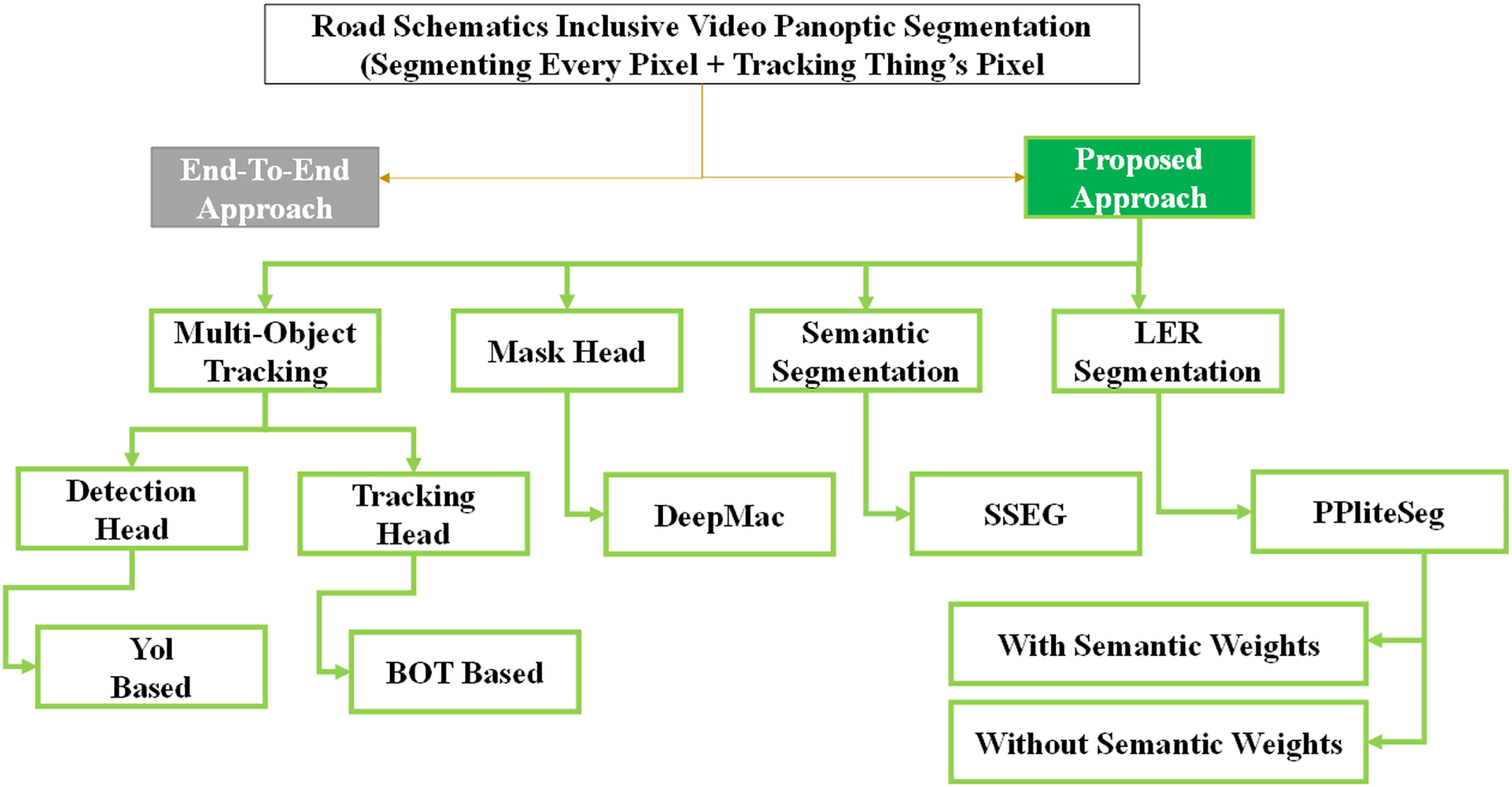
VPS task takes videos as input and returns class and tracking ID for every pixel of an image in the input video. Though all the pixels are assigned a class ID, a tracking ID, or object ID is assigned only for thing classes and not for stuff regions. The stuff segments are dealt with by the networks at the pixel level (Cheng et al., 2019; Li et al., 2022; Xiong et al., 2019). In this work, the lane regions are under the stuff regions but have three distinct patches, namely the ego-lane, left lane, and right lane. For all the other stuff regions, an encoder-decoder semantic segmentation branch is the choice to classify the pixels and discriminate segments with no assignment of an object ID. This heterogeneous nature of the output intuitively facilitates joint learning. Joint learning demands the feature extractor to strike a tradeoff between object-ness of region of interest (ROI) (things) and pixel classification (stuff). Jointly learning them in a unified setup necessitates the feature extractor to deal with the tradeoff between its orientation towards either objects of ROI (things) or pixel classification (stuff). Joint learning constrains the network to agree upon these two different representations. Joint learning of heterogeneous subtasks of VPS tends to degrade the single-task performances. Moreover, in literature, many networks (Weber et al., 2021; Xiong et al., 2019; Yang, Fan & Xu, 2019) initially performed image panoptic segmentation on a single frame of the video using the image panoptic segmentation branch of the network and then performed tracking on the instances obtained from them using the tracking branch. Many of these networks share features among the branches in a complex way. Many networks decouple the VPS task at the branch level, but the image panoptic segmentation and tracking are decoupled. The actual heterogeneous tasks, such as semantic segmentation and instance segmentation, are again learnt in joint learning. This work proposes to decouple the VPS task into (i) segmentation of stuff and (ii) tracking and segmentation of things. The subtasks of the VPS are realized by various state-of-the-art networks trained on task-specific datasets. This decoupling facilitates the separation of feature extractors for semantic segmentation and tracking, in turn, dealing with the heterogeneous subtasks separately. The decoupling takes advantage of the multiple task-specific datasets for training, thus enabling the network to have better generalization. The tasks, such as tracking and semantic segmentation, have larger task-specific datasets than VPS datasets and are tailored for the specific task, thus enabling better benchmarking. The decoupled setup gives the opportunity to incorporate lane semantics such as drivable area segmentation, road marking, lane classification, etc., into the VPS task, making it a complete scene understanding task. Figure 1 shows the proposed approaches utilizing various state-of-the-art networks for different tasks. The inherent merits of each of the methods are exploited to get the VPS inclusive of lane semantics.
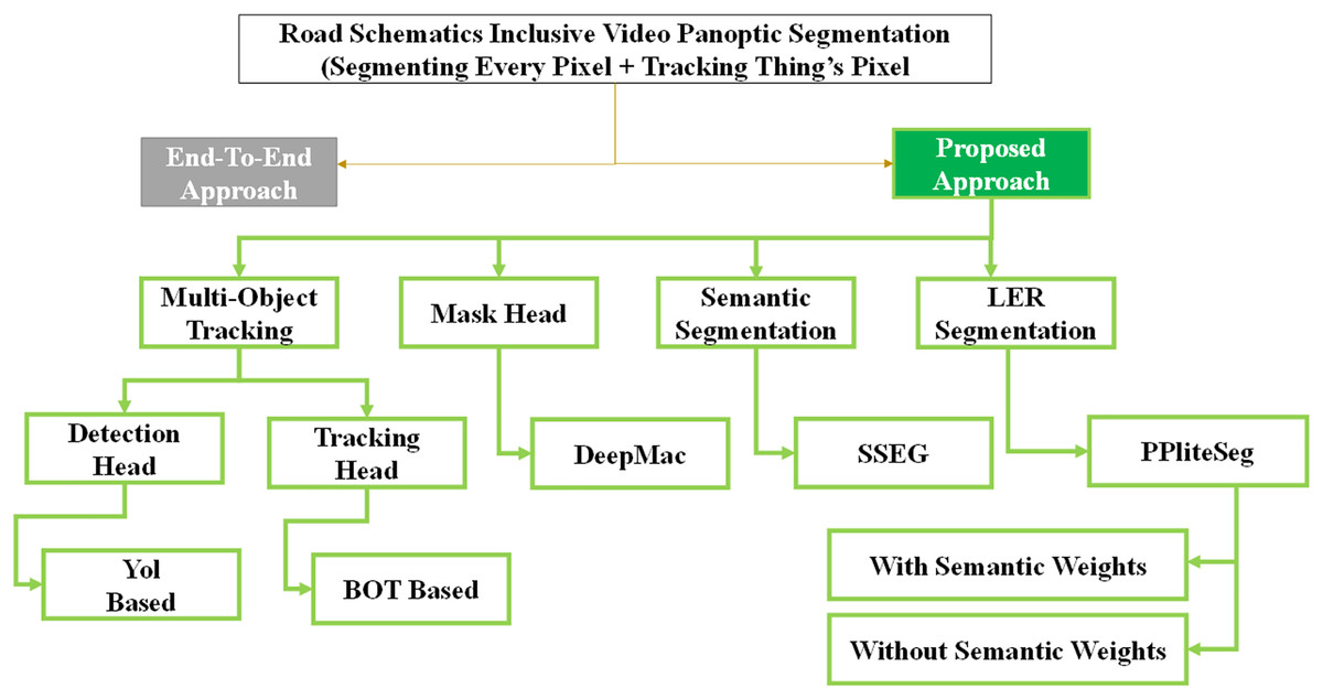
Figure 1: Proposed approach for fusing lane-semantics into VPS task.
All the deep learning network training and inferences are performed on a desktop PC with AMD Threadripper 1900x with 32 GB RAM and RTX 3090 GPU. The software suite comprises a Ubuntu 18.04 operating system with CUDA tools for GPU acceleration. Anaconda Python is used as the Python distribution with specific APIs such as Pytorch, Tensorflow, and Paddleseg used for the various tasks involved.
Decoupling things and stuff handling
The tracking of things is posed as a Multiple Object Tracking problem. The tracking of things is addressed using the multiple objects tracking (MOT) route. Tracking algorithms adopt many proven methods like the Kalman filter for trajectory prediction, Siamese networks for similarity learning, long short-term memory (LSTM) to estimate motion, IoU matching to match detections with tracks, attention mechanisms to find spatiotemporal pixel/feature interactions, ReID to improve object reidentification, etc. In the proposed approach, BoTSORT (Aharon, Orfaig & Bobrovsky, 2022) is adopted for the MOT task. The tracking of things is posed as a multiple-object tracking problem in the proposed approaches. Multiple object tracking has a vast literature, utilizing a variety of methods to solve it. Many tracking algorithms utilize many well-proven methods, like IoU matching to match detections with tracks, Kalman filter for trajectory prediction, attention mechanisms to find spatiotemporal pixel/feature interactions, Siamese networks for similarity learning, LSTMs to estimate motion, ReID to improve person reidentification, etc. In this work, two networks with two different tracking methods are utilized. For the MS approach, the architecture PCAN (Prototypical Cross Attention Network) is chosen to perform the Multiple Object Tracking and Segmentation (MOTS) task, and for the MIS approach, BoTSORT is chosen to perform the MOT task (Aharon, Orfaig & Bobrovsky, 2022).
Segmentation of detected and tracked bounding boxes at each frame is handled by DeepMac (Zhou, Wang & Krähenbühl, 2019). DeepMAC is a class-agnostic instance segmentation network built on CeterNet by introducing a mask head to generate instance masks (Zhu et al., 2018). A modified version of the deep hourglass network is used as the mask head. DeepMAC is popular for its characteristic of attaining strong mask generalization for unseen classes, which was trained on the COCO dataset.
Multiple object tracking using tracking-by-detection
BoTSORT is an example of a tracking-by-detection-based tracker based on ByteTrack (Zhang et al., 2022). It uses a modified Kalman filter to estimate the dimensions of the bounding box rather than the aspect ratio. Camera motion is compensated using an image registration technique, and fusion of the IoU-ReID cosine distance function is used to find the similarity between the detected boxes and predicted boxes. A ReID module with ResNet50 as the backbone is used for the reidentification of the object. Data association of detected boxes with lower scores caused by occlusion, motion blur, and changes in the size of the objects is handled by ByteTrack. The BoT-SORT network was originally trained on MOT16 (Milan et al., 2016) dataset, and the detection head YOLOV7 (Lin et al., 2014) was trained on COCO dataset (Birodkar et al., 2021), giving it the ability to track multiple classes.
Segmentation of stuff
DeepLab v3 + semantic segmentation network is utilized to segment the stuff regions. The network was trained on a large-scale augmented training dataset developed by synthesizing novel training samples using a video prediction-based methodology (Zhu et al., 2018). Additionally, augmentation was carried out from Cityscapes and KITTI datasets, thereby enabling high generalization capability. The segmentation of the LER and DAD lane features is carried out using the custom LER dataset and the original BDD Drivable area detection dataset, respectively.
All the methods for detection and segmentation are selected based on the criteria of real-time performance with a minimum of 60 FPS and 70% mAP. This is a reasonable selection criterion considering that the intended application is autonomous driving.
Merging things and stuffs
There are no conventional preprocessing methods applicable to the proposed work. General regions belonging to stuff classes and the road regions from the LER classes or DAD classes are combined with instance masks of thing classes associated with track IDs from tracking networks at the image level to generate VPS. The stuff segments are placed on a blank array, then the things masks are placed on top of it, overwriting pixels of stuff where they overlap.
The algorithm for merging things and stuff is as follows.
-
i.
Create an empty array of size M × N × 3, IVPS.
-
ii.
Obtain class agnostic instance segmentation inference IIS from DeepMac.
-
iii.
Assign the class ID and track ID from the Yolo-BOTSORT inference for every mask based on the order of the masks’ column indices in the image.
-
iv.
Identify overlapping pixels of two objects from the things class in the instance-segmented image.
-
v.
Address overlaps between two masks in an image by prioritizing the mask that carries the highest-class confidence as inferred by Yolo-BOTSORT.
-
vi.
Obtain Semantic Segmentation inference from SSEG ISS
-
vii.
For all stuff pixels from ISS, copy the pixels (i, j) from IVPS(i, j) = ISS(i, j)
-
viii.
For all things classes from IIS, copy the pixels (i, j) from IVPS(i, j) = IIS(i, j)
-
ix.
Convert COCO dataset format class IDs from YoloV5-BOTSORT to City-scapes convention, since YoloV5 is trained with the COCO dataset.
-
x.
Overlapping regions of things and stuff are addressed by prioritizing the things class from IIS, since classes and instances are extracted from IIS.
-
xi.
Replace pixels from road segments with LER segments.
-
xii.
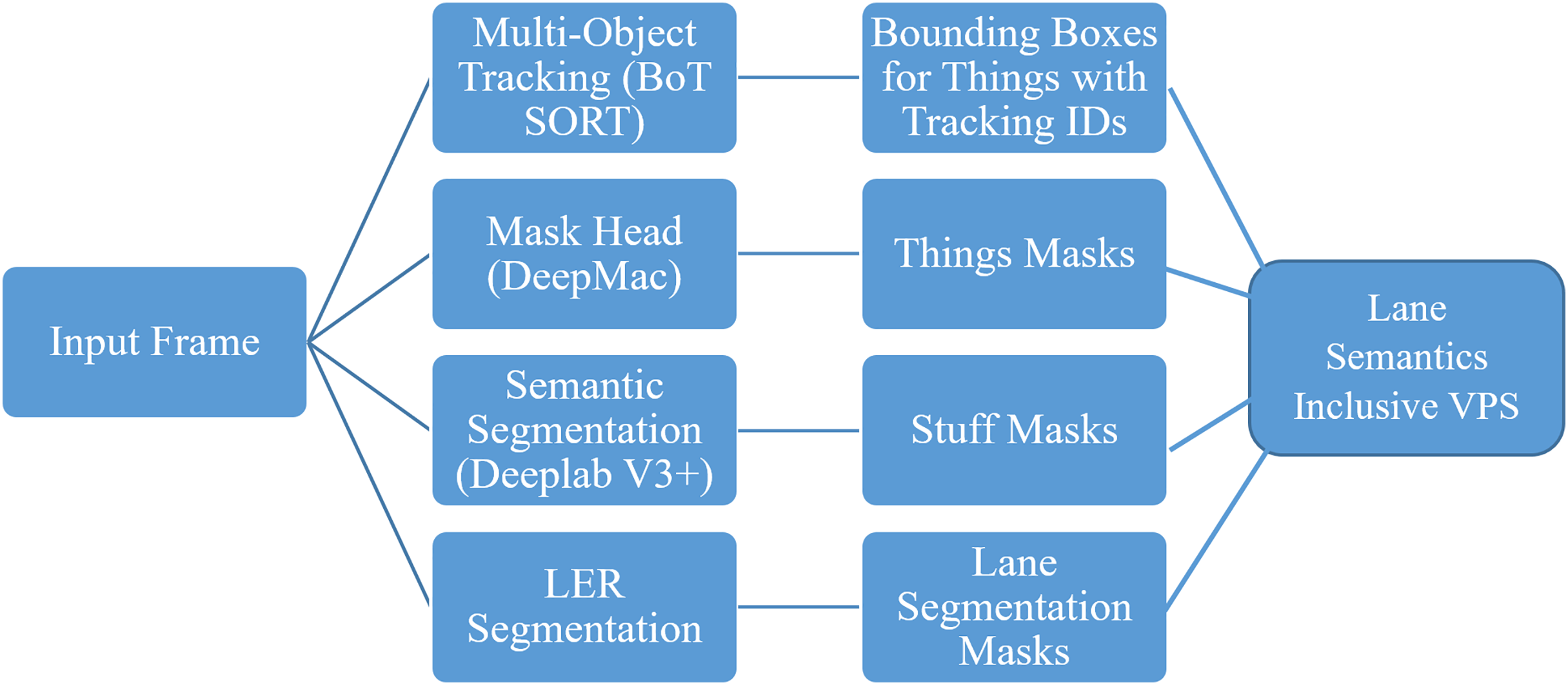
Handle non-overlapping regions between SSEG and LER segmentation results with eight connectivity evaluation. The process flow of the approach to obtain VPS output is given in Fig. 2.
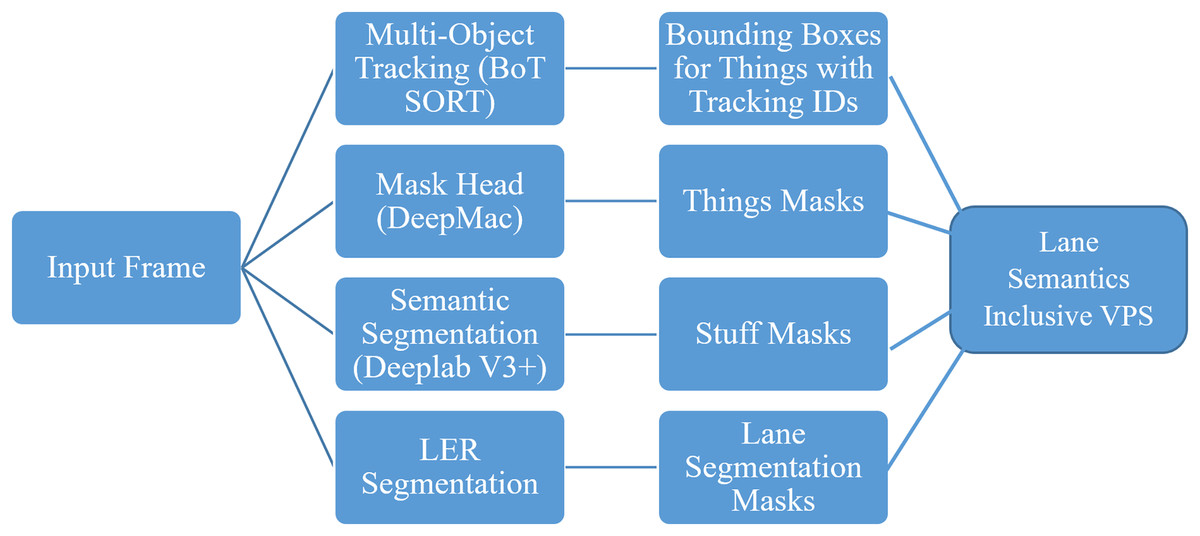
Figure 2: Proposed decoupled pipeline for lane-semantics inclusive VPS.
Any state-of-the-art tracking algorithm or semantic segmentation network can be incorporated as a sub-task to realize the VPS task in this manner. These network weights are as provided by the original works, and no fine-tuning is done.
LER segmentation
The LER segmentation is achieved through a structured approach in this work. The LER segmentation does not involve any data pre-processing. The raw RGB image from the camera can be fed to the semantic segmentation network. Multiple state-of-the-art deep learning methods for semantic segmentation were evaluated to understand the suitability of the method for LER segmentation. A custom criterion is used for choosing the right network based on the right balance between time performance and accuracy. The evaluation metric most used for semantic segmentation networks is mean average precision (mAP) and frames per second. Methods exhibiting an mAP greater than or equal to 70% and a minimum of 60 FPS inference speed on a GTX 1080Ti are set as a threshold for choosing the candidate methods for training on the LER dataset. The criteria are verified against benchmarks reported on the Cityscapes semantic segmentation dataset. By current standards of inference using hardware such as the NVIDIA Drive platform, a network of this level of competency can be considered as affordable for real-world implementation. All the initially chosen networks are trained with the settings reported by the authors of the work for a minimum of 50 epochs with the respective trained initial weights. The networks are verified for good performance based on the metric mean Intersection over Union (mIoU) on the validation dataset. A threshold of minimum mIoU of 50% is chosen to consider the networks as good-performing ones. The initial evaluation is performed on the DAD dataset from the original BDD100K dataset.
To demonstrate the methods’ capabilities to adapt to newer classes that are just in a different spatial location in the image (the left and right lanes) as compared to those in the DAD dataset (the adjacent lanes alone), the performance evaluation is performed on both datasets. The chosen networks are subject to training on both datasets using the same combinations of hyperparameters and loss functions. Training on both datasets presents an opportunity to evaluate the ego-lane-centric direction learning capability of the networks. The novelty in the proposed approach related to LER segmentation is the utilization of semantic weights in the loss functions during training. This is used primarily to address the direction-contextual misclassification, which may either be right lane classified as left or vice versa. All the shortlisted networks are trained for a minimum of 200 epochs with and without semantic weights, which allows us to establish the role of semantic weights in improving networks’ accuracy. All the numerical evaluations are reported based on the results obtained on the test set of the datasets.
Code and data availability
The code and dataset are available at GitHub: https://github.com/SubhasreePasupathi/LER_Segmentation.
(All the codes and datasets used in the research work presented in this article are linked in the above GitHub repository. Refer to the readme file. The LER dataset label created by this work were made available for public access (DOI: 10.5281/zenodo.17768440). The original drivable area detection annotations, which were modified to this LER segmentation, can be downloaded from https://bdd-data.berkeley.edu. (DOI: 10.1109/CVPR42600.2020.00271)).
LER dataset
Any deep learning method’s performance is thoroughly based on the quality and the quantity of the dataset. The LER segmentation dataset is prepared based on a semi-automated approach that modifies the BDD100K DAD dataset to decompose the adjacent lanes class into left and right lanes. As explained in the methodology section of the article, both datasets are utilized as part of the research work to understand the learning ability of newer classes.
BDD100K is a large-scale dataset comprising diverse driving videos and annotations for different tasks such as object detection, semantic segmentation, instance segmentation, DAD, lane marking, MOT, and MOTS. In this research work, the DAD annotations are modified to form a new dataset, which is termed the LER dataset. The main purpose of choosing the BDD100K dataset is its diversity in terms of scene types, weather conditions, and quantity. For any long-term autonomy to work satisfactorily, it is imperative for a machine learning model to be trained with a dataset with such diversity. The original dataset comprises 1,00,000 images for DAD, which is split into training (70,000), validation (10,000), and testing (20,000). Since the original DAD is modified into the LER dataset, the testing set usage is not applicable for the current research work; hence, the original training set is divided into 60,000 for the actual training set and 10,000 for the test set. To ensure a comparable basis, the same set is also used for training the DAD task as well as the LER segmentation tasks.
In the original DAD dataset from BDD100K, the drivable lanes are divided into two different categories, namely directly drivable area and alternatively drivable area. The directly drivable area is the region where the ego-vehicle is currently being driven on, while the alternate drivable area is a lane the ego-vehicle might drive on by performing lane changes. The two drivable areas are visually distinguishable, but the functionality of the lanes is different, demanding the algorithms to recognize vehicles on the respective lanes and understand the context of the transaction. The following plots present some of the vital statistics of the subset of the BDD100K used for both the DAD and LER segmentation tasks.
Though it might look like converting DAD annotations to LER segmentation can be automated, no hardcoded logic will be able to accomplish this. This is because the nature of lanes is geometrically diverse, so they cannot fit under any plausible assumption. Since the dataset comprises 80,000 images (including the original BDD100K’s train and validation set alone), the task of manually annotating is time-consuming. Hence, a hybrid strategy of annotating initially using a hardcoded logic that may assign the alternative lanes as either left or right lanes, which is expected to have segments that are misclassified. Careful manual scrutiny of all the automatically generated annotations is made, and the necessary corrections of the misclassified patches are carried out. The algorithm for the automated annotation attempt is presented below:
-
i.
Collect the individual regions’ pixel coordinates from the DAD dataset.
-
ii.
Verify the column coordinates to be greater than the centroid for the alternate regions’ pixel coordinates.
-
iii.
If the condition is satisfied, assign the right class label for the same.
-
iv.
If not, assign the left class label.
As it may be observed, the algorithm is rudimentary, which cannot handle cases such as lanes that are not observed from the center of the field of view, lanes that are curving either to the left or right, etc. All those cases are manually reannotated, and the entire annotations are verified for correctness. The verification process involved multiple people manually observing the RGB and label image pair (in color) placed adjacent to each other to avoid any fatigue-based misses. A few sample images illustrating the misclassified segments along with the manually corrected ones are presented in Fig. 3. It can be appreciated that the nature of these cases is so diverse that no hard-coded logic can classify the ego alternate lanes to LER lanes. Additionally, the originally annotated images had annotation errors, especially notable ones are for the images from night driving conditions. These errors are corrected both in the DAD and LER datasets to arrive at the final dataset. The second row in Fig. 3 is an example of such an error from the BDD100K annotators.
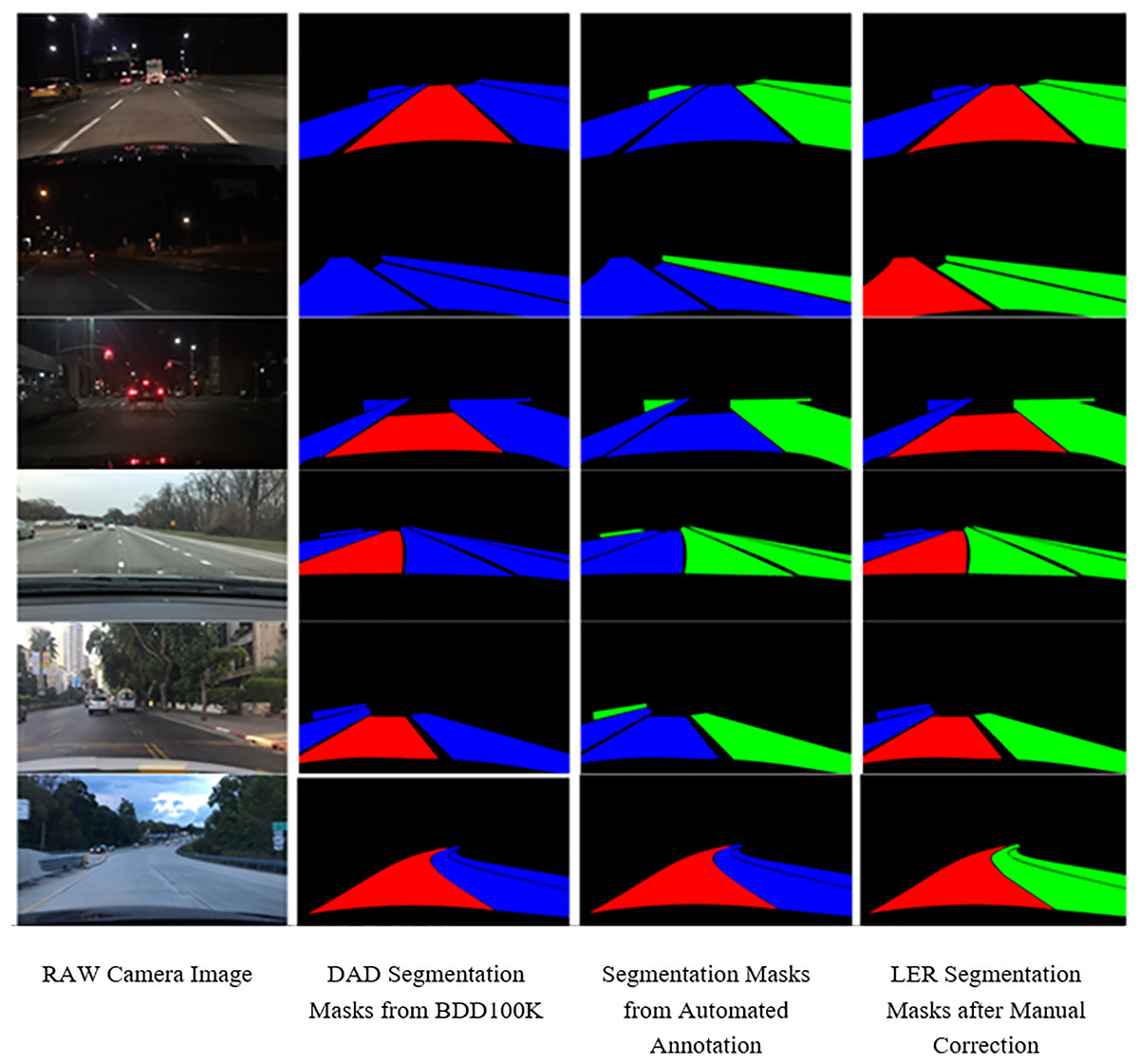
Figure 3: Sample images column (first column) RAW camera image (second column) DAD segmentation masks from BDD100K (third column) segmentation masks from automated annotation (fourth column) LER segmentation masks after manual correction.
Copyright: The Regents of the University of California.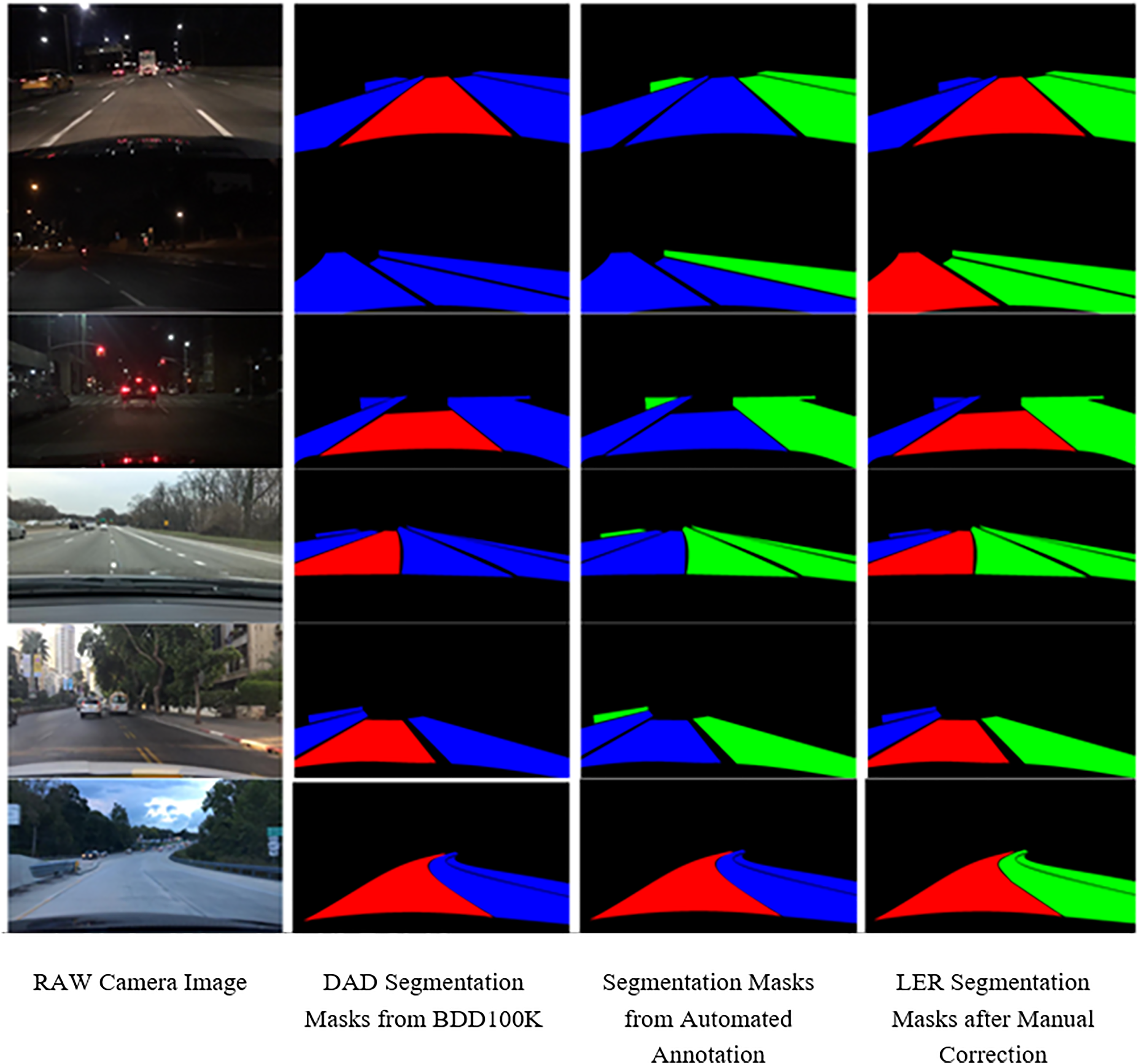
The number of iterations of training is chosen based on the batch size of each network, resulting in approximately 230 epochs. There was no early stopping strategy used; only the best weights based on reduction in validation loss were used. This is reasonable since learning rate decay is used, which could potentially result in finer convergence. All the weights are saved in the standard ‘.pdparams’ and ‘.pdopt’ files, followed by the Paddlepaddle API. All the metrics computed on the training dataset, such as loss, batch cost, etc, and metrics on the validation dataset, such as mIoU, Accuracy, and Kappa, are logged for every 10 iterations.
Based on the preliminary training, the PPLiteSeg family (Fan et al., 2021) is identified as a network of choice. The superior performance, mainly in the context of mIoU and the number of epochs required to achieve a larger mIoU, is the primary reason to select the network.
The model and training specifications of PPLiteSeg are as follows. The batch size is 16. The optimizer used is the ADAM optimizer with weight decay to 1e−4. The starting learning rate is set at 1e−5. The loss function used is Ohem cross-entropy loss. For transformation, step scaling is used with a minimum step scale factor of 0.125, a maximum scale factor of 1.5, and a step size of 0.125. The input crop size is 1,024 × 512. Transforms applied were random horizontal flipping, random distort, with brightness range as 0.5, contrast range as 0.5, and saturation range as 0.5. The backbones used are STDC1 and STDC2 (Ke et al., 2021). The different input scales taken for training are 0.5, 0.75, and 1.0.
Evaluation method and metrics
One of the fundamental issues in the LER segmentation is the nature of lanes, which are bland and textureless. The lane markings are the only texture-inducing feature in the images. This makes the problem of LER segmentation an ego-lane-centric relative direction learning problem from bland features. Due to this nature, the chances for misclassification are very high. Misclassifications such as ego classified as right and vice versa, left classified as ego and vice versa, and in some cases right as left and vice versa. These issues were encountered during the preliminary training with the DAD dataset, too. A novel approach of semantic weights during the training process is utilized to mitigate the issue. Semantic weights are weights that scale the loss for every pixel. Semantic weights are an array of scalar values of the same size as the ground truth label for semantic segmentation. The semantic weights are implemented during training as a scalar multiplication in an element-wise manner between the actual loss computed and the semantic weights array as follows: Final loss = loss × semantic weights.
A nonuniform semantic weighing strategy is conceived as per the following weight assignment. Such a strategy is reasonable since the very purpose of LER-like segmentation is to clearly distinguish the lanes, and misclassifications related to the lane classes are not permissible.
As presented in Table 1, three different semantic weights are evaluated to understand the role of the relative magnitudes of the semantic weights in mitigating the issue of misclassification. (0.25, 0.5, 1), (1, 2, 3) and (1, 4, 8) are the semantic weights chosen based on the severity of misclassification. It may be observed from Table 1 that the misclassification among the left and right classes is penalized more heavily than the other possibilities.
| Actual class | Predicted class | Error server key |
Semantic weights | ||
|---|---|---|---|---|---|
| Type 1 | Type 2 | Type 3 | |||
| Left | Ego | Medium | 0.5 | 2 | 4 |
| Right | Ego | 0.5 | 2 | 4 | |
| Ego | Left | 0.5 | 2 | 4 | |
| Ego | Right | 0.5 | 2 | 4 | |
| Right | Left | High | 1 | 3 | 8 |
| Left | Right | 1 | 3 | 8 | |
| Ego | Background | Low | 0.25 | 1 | 1 |
| Left | Back | 0.25 | 1 | 1 | |
| Right | Background | 0.25 | 1 | 1 | |
| Background | Ego | 0.25 | 1 | 1 | |
| Background | Left | 0.25 | 1 | 1 | |
| Background | Right | 0.25 | 1 | 1 | |
The evaluation method adopted in this work basically attempts to demonstrate the effectiveness of semantic weights by comparing the results of the model trained with a semantic weights-incorporated loss function against plain loss functions. Additionally, two different semantic weight combinations are also attempted to evaluate the role of the magnitude of the semantic weights in penalizing misclassifications. To understand the performance of the novel implementation of the semantic segmentation network for LER segmentation tasks applied with and without semantic weights, the following performance evaluation metrics are used. All the metrics are computed on a fixed test set in the LER segmentation dataset. The various notations used in the expressions are as follows:
n = number of classes
pij = number of pixels of class i predicted as class j
pii = number of correctly predicted pixels for class i (true positives)
ti = total number of pixels belonging to class i
p⋅j = total number of pixels predicted as class j
N = total number of pixels across all classes
Average precision
The average precision is computed from the precision-recall curve as follows:
where P(r) is the precision at the recall level. In the current case of semantic segmentation of LER classes, AP is computed for each class and averaged in order to perform per-class evaluation.
Average recall
The average recall is computed as follows:
F1-score
The article reports the average F1-score for the semantic segmentation, wherein the F1-score for every class is computed as follows:
The macro average reported in the next section is computed as follows:
Pixel accuracy
The pixel reported for the semantic segmentation is computed as follows:
Mean accuracy
The mean accuracy is computed as follows:
Mean IoU
The IoU is computed as follows:
From which the Mean IoU is computed as follows:
Weighted IoU
The weighted IoU is computed based on the weights, which are in turn based on the number of pixels per class.
Results
The experimental results obtained are shown in the form of performance evaluation metrics of LER segmentation for different configurations of the network, and the combinations of semantic weights are presented in Table 2. The metrics were obtained on the test set of the LER dataset comprising 10,000 examples. The average results are presented in Table 2. As mentioned earlier, combinations of three different scales and three different semantic weights are used. The scales are represented in Table 2 as Scale 0.5, Scale 0.75, and Scale 1.0. The semantic weights are represented as plain, 123, and 148, where plain refers to no semantic weights applied in the Ohem Cross Entropy Loss. The semantic weights (1, 2, 3) and semantic weights (1, 4, 8) are applied as per Table 1 to magnify the critical misclassification, ensuring adequate compensations during training.
| Metrics | STDC2 | ||||||||
|---|---|---|---|---|---|---|---|---|---|
| Scale 0.50_ plain | Scale 0.50_ 123 | Scale 0.50_ 148 | Scale 0.75_plain | Scale 0.75_ 123 | Scale 0.75_148 | Scale 1.0_ plain | Scale 1.0_ 123 | Scale 1.0_ 148 | |
| Average precision | 0.820334 | 0.854468 | 0.863136 | 0.859263 | 0.862385 | 0.84544 | 0.86485 | 0.864883 | 0.864728 |
| Average recall | 0.806891 | 0.827016 | 0.840857 | 0.839735 | 0.847915 | 0.829619 | 0.846085 | 0.842728 | 0.841155 |
| F1-score | 0.799862 | 0.827975 | 0.843199 | 0.839561 | 0.846305 | 0.828693 | 0.84641 | 0.845136 | 0.844008 |
| Pixel accuracy | 0.955257 | 0.958388 | 0.962449 | 0.960084 | 0.961796 | 0.960508 | 0.960837 | 0.962838 | 0.963156 |
| Mean accuracy | 0.88775 | 0.87612 | 0.893647 | 0.886484 | 0.893047 | 0.897226 | 0.888035 | 0.895173 | 0.895397 |
| Mean IoU | 0.830743 | 0.8301 | 0.850858 | 0.840422 | 0.846983 | 0.849827 | 0.842276 | 0.852325 | 0.853388 |
| Weighted IoU | 0.929499 | 0.929612 | 0.936999 | 0.933981 | 0.93607 | 0.93504 | 0.935182 | 0.937399 | 0.938063 |
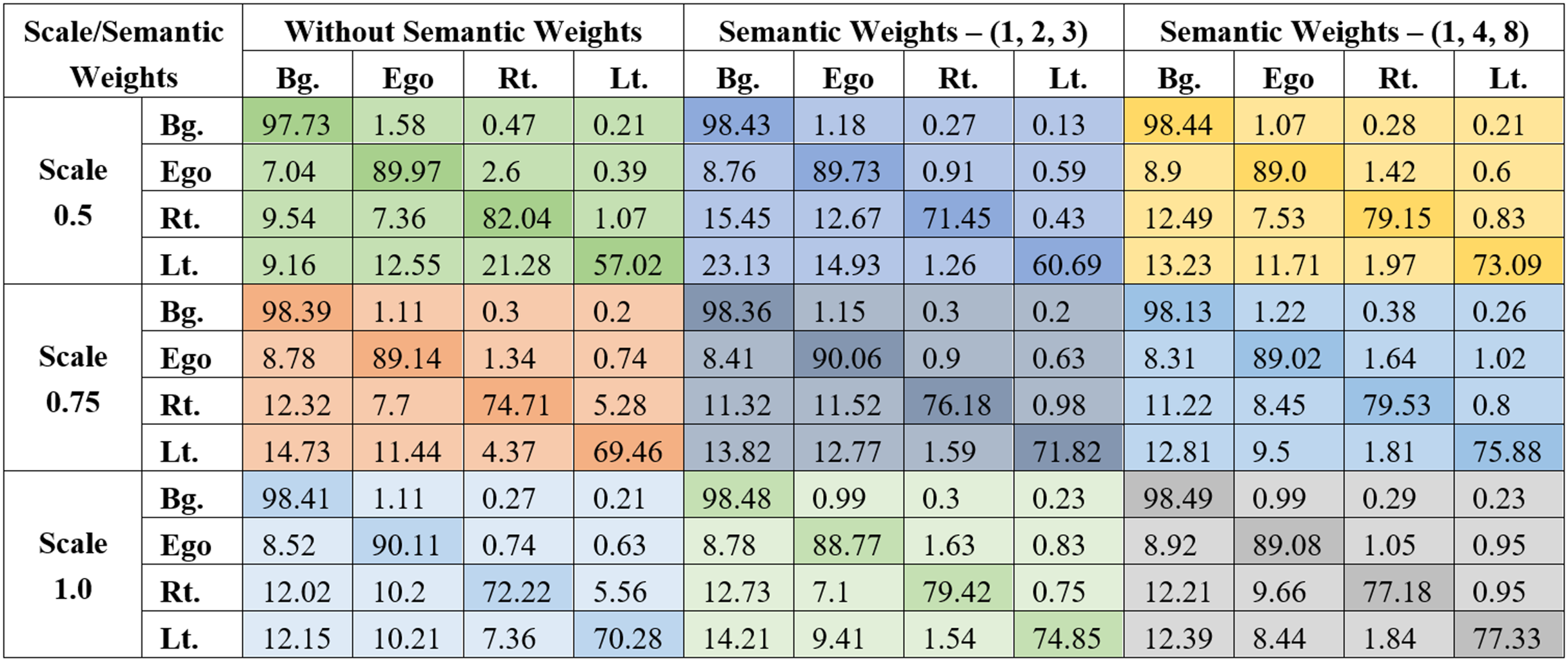
The evaluation parameters are derived from the confusion matrices corresponding to each combination shown in Fig. 4. In these matrices, a strong diagonal presence reflects accurate classifications, while the off-diagonal elements represent misclassifications between different classes. All combinations have been trained using the STDC2 backbone.
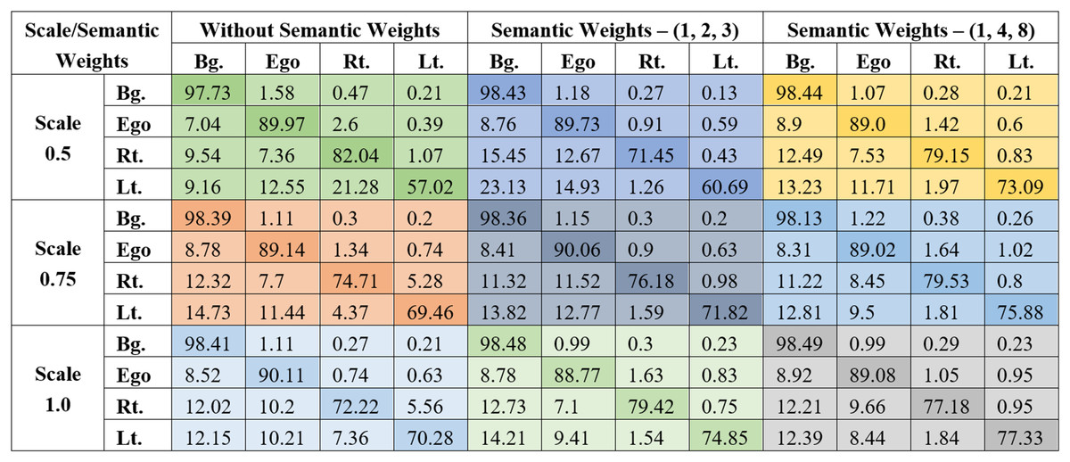
Figure 4: Confusion matrices are obtained for the entire test of the LER dataset.
In order to highlight the significance of the results, confidence intervals and values based on the Wilcoxon Single Rank Test are computed. The confidence intervals were obtained based on the bootstrapping method with 1,000 bootstrap samples on the test set. The resampled distribution of each metric allows for computing the 2.5th and 97.5th percentile (95% confidence interval, the most common interval for semantic segmentation on large datasets). The confidence intervals are rounded off to three decimal places for the sake of brevity in presentation, as observed in Table 3.
| Metrics | STDC2 | |||||||||||||||||
|---|---|---|---|---|---|---|---|---|---|---|---|---|---|---|---|---|---|---|
| Scale 0.50_ plain | Scale 0.50_ 123 | Scale 0.50_ 148 | Scale 0.75_plain | Scale 0.75_ 123 | Scale 0.75_148 | Scale 1.0_ plain | Scale 1.0_ 123 | Scale 1.0_ 148 | ||||||||||
| 95% confidence intervals | ||||||||||||||||||
| Lower | Upper | Lower | Upper | Lower | Upper | Lower | Upper | Lower | Upper | Lower | Upper | Lower | Upper | Lower | Upper | Lower | Upper | |
| Average precision | 0.814 | 0.826 | 0.849 | 0.860 | 0.858 | 0.868 | 0.855 | 0.864 | 0.858 | 0.867 | 0.841 | 0.850 | 0.860 | 0.870 | 0.861 | 0.869 | 0.861 | 0.868 |
| Average recall | 0.801 | 0.813 | 0.822 | 0.833 | 0.836 | 0.846 | 0.835 | 0.845 | 0.843 | 0.853 | 0.825 | 0.835 | 0.841 | 0.852 | 0.838 | 0.848 | 0.837 | 0.845 |
| F1-score | 0.794 | 0.806 | 0.822 | 0.834 | 0.838 | 0.849 | 0.835 | 0.844 | 0.842 | 0.851 | 0.824 | 0.834 | 0.842 | 0.851 | 0.841 | 0.850 | 0.840 | 0.849 |
| Pixel accuracy | 0.951 | 0.959 | 0.955 | 0.962 | 0.959 | 0.966 | 0.957 | 0.963 | 0.959 | 0.965 | 0.958 | 0.963 | 0.959 | 0.963 | 0.961 | 0.965 | 0.961 | 0.965 |
| Mean accuracy | 0.884 | 0.892 | 0.871 | 0.881 | 0.889 | 0.899 | 0.882 | 0.891 | 0.888 | 0.898 | 0.893 | 0.902 | 0.883 | 0.894 | 0.890 | 0.900 | 0.890 | 0.899 |
| Mean IoU | 0.827 | 0.835 | 0.827 | 0.834 | 0.847 | 0.855 | 0.836 | 0.845 | 0.842 | 0.852 | 0.845 | 0.855 | 0.837 | 0.848 | 0.847 | 0.857 | 0.848 | 0.858 |
| Weighted IoU | 0.926 | 0.933 | 0.926 | 0.933 | 0.934 | 0.941 | 0.931 | 0.938 | 0.933 | 0.940 | 0.932 | 0.939 | 0.931 | 0.939 | 0.934 | 0.941 | 0.934 | 0.941 |
P-values are obtained to demonstrate the role of the semantic weights. The p-values are obtained based on a paired-test (Wilcoxon signed-rank test) conducted between the plain version of the network and the semantic weights implemented versions for the corresponding scale. The p-values are computed based on the null-hypothesis that there is no difference between the performance metrics of the two algorithms. Hence, smaller p-values (<0.05) indicate that the results from the two algorithms are not similar and vice versa. This pair-wise comparison between the vanilla version and the semantically weighed versions demonstrates the effectiveness of the semantic weights for the LER segmentation tasks, which is pivotal to this work. The pairwise p-values are presented in Table 4.
| Metrics | Scale 0.50_ plain vs. Scale 0.50_123 |
Scale 0.50_ plain vs. Scale 0.50_148 | Scale 0.75_plain vs. Scale 0.75_123 | Scale 0.75_plain vs. Scale 0.75_148 | Scale 1.0_ plain vs. Scale 1.0_123 | Scale 1.0_ plain vs. Scale 1.0_148 |
|---|---|---|---|---|---|---|
| Average precision | 1.2e−04 | 6.2e−05 | 0.184 | 0.034 | 0.842 | 0.614 |
| Average recall | 3.4e−03 | 4.8e−03 | 0.021 | 0.072 | 0.056 | 0.043 |
| F1-score | 8.7e−04 | 9.1e−04 | 0.049 | 0.018 | 0.119 | 0.162 |
| Pixel accuracy | 1.1e−02 | 0.021 | 0.093 | 0.462 | 0.037 | 0.018 |
| Mean accuracy | 0.19 | 0.13 | 0.012 | 0.041 | 0.021 | 0.006 |
| Mean IoU | 0.71 | 0.047 | 0.067 | 0.087 | 0.081 | 0.039 |
| Weighted IoU | 0.62 | 0.082 | 0.241 | 0.291 | 0.266 | 0.071 |
The following observations are made concerning the impact of scale: an overall trend indicates that increasing the scale consistently enhances all evaluation metrics, with notable improvements in Average Precision and IoU metrics—both of which are particularly crucial in the context of LER segmentation for autonomous driving applications. Despite varying semantic weight combinations, a degree of confusion between the L and R classes persists. However, this confusion tends to diminish at higher scales. Utilizing full-scale input alongside elevated semantic weights equips the model with both enhanced spatial resolution and targeted learning capacity, enabling more effective differentiation between challenging classes, especially L and R.
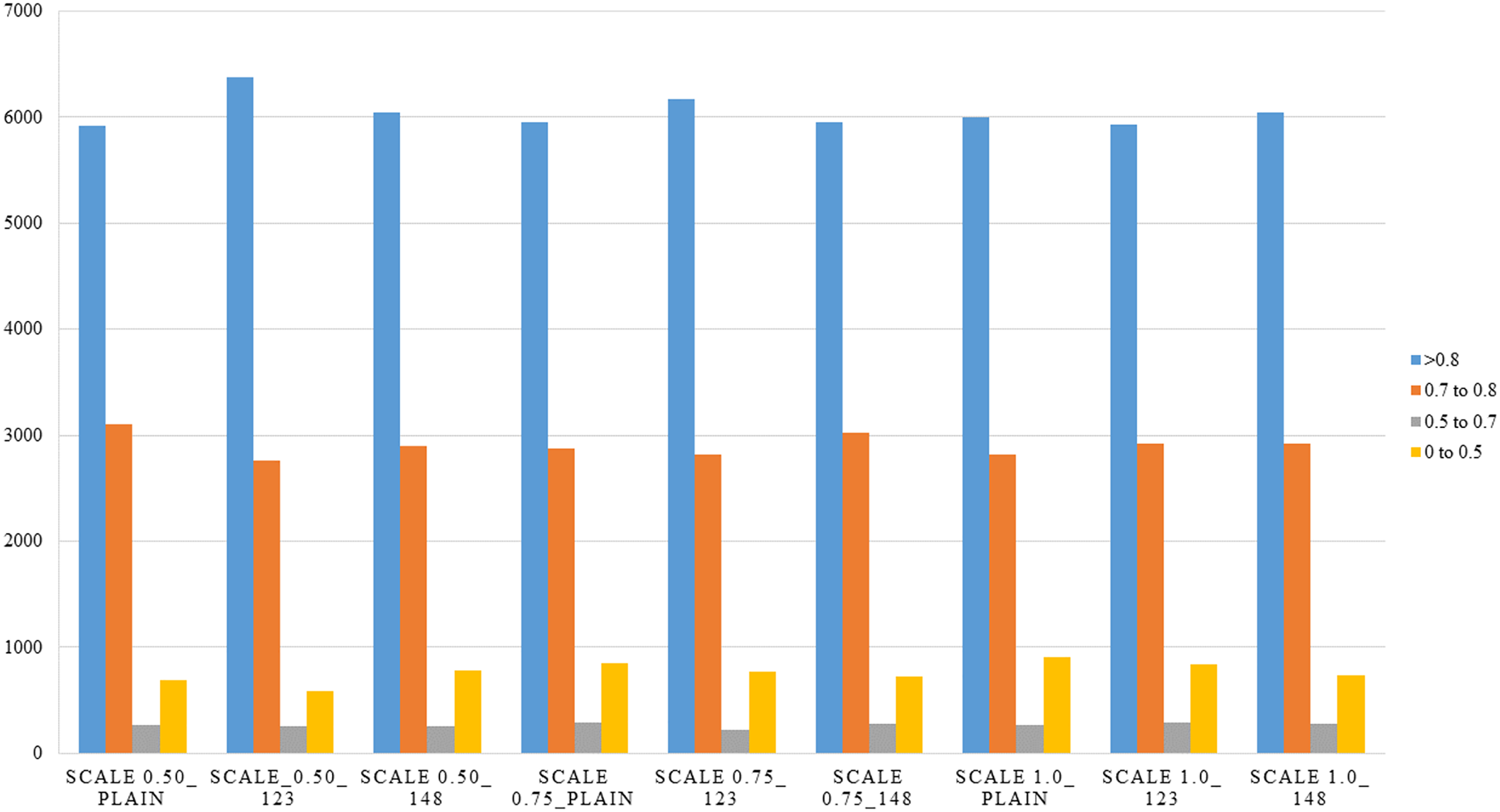
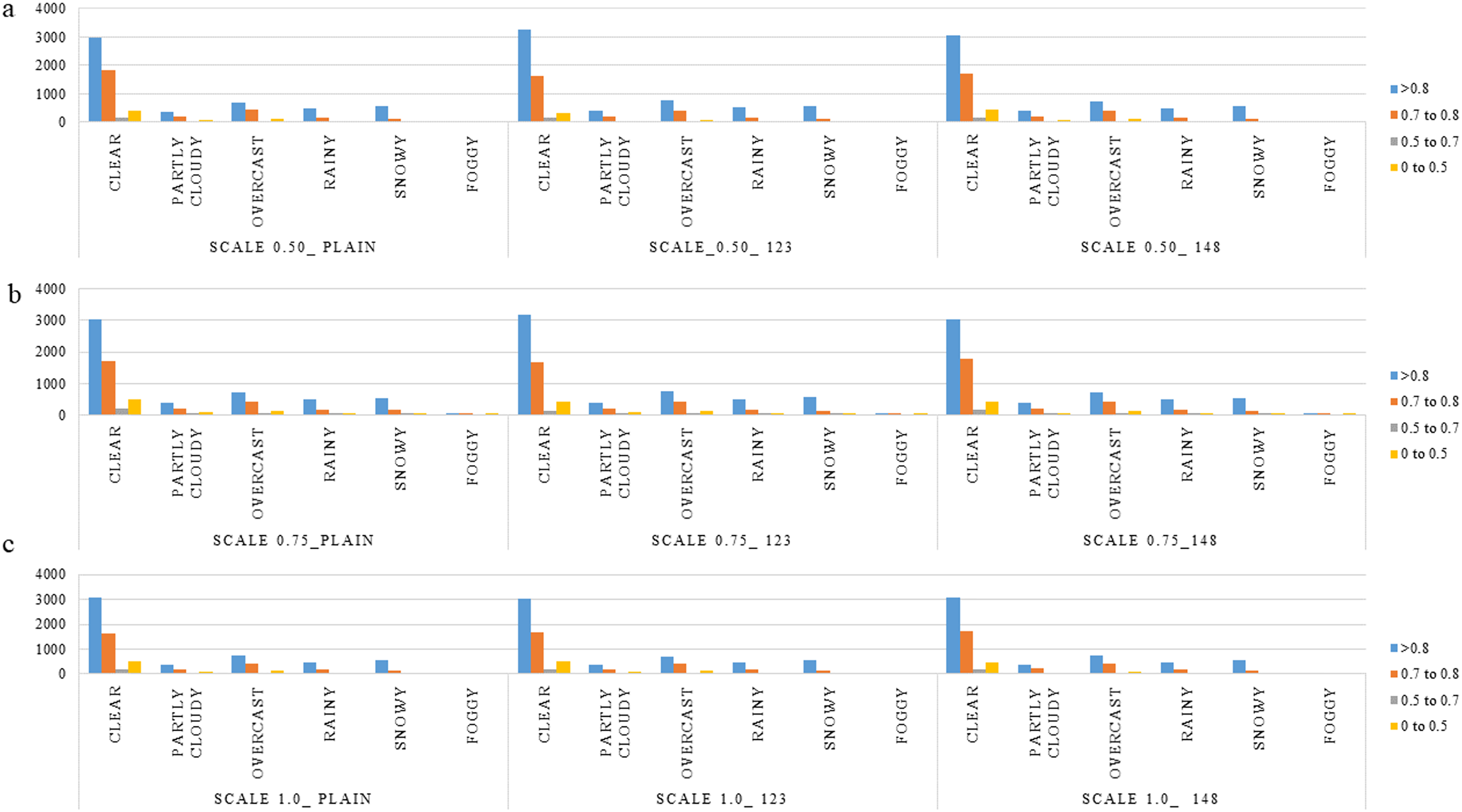
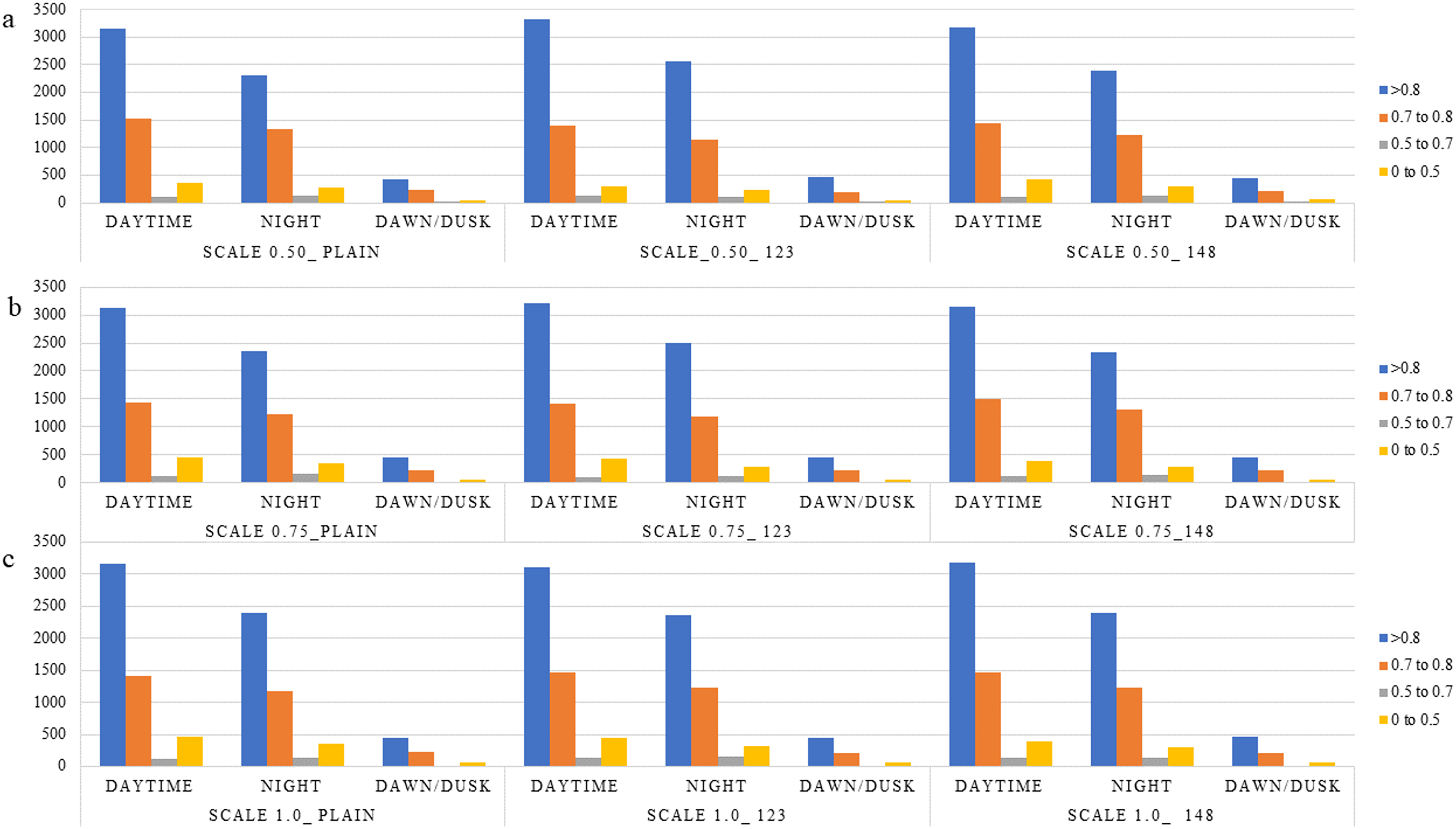
The observed behavior is consistent with expectations regarding the influence of the scale parameter in the PPLiteSeg-STDC2 network. Larger input scales inherently retain a greater degree of spatial detail, which plays a crucial role in enabling the model to capture and learn finer structural patterns within an image. This is particularly important in the context of LER (Left, Edge, Right) segmentation, where accurately delineating the often subtle boundaries between the L, E, and R classes is essential for robust autonomous driving systems. Among the tested configurations, the network demonstrates a clear advantage when operating at scale 1.0 compared to reduced scales such as 0.5 and 0.75. The higher scale facilitates richer spatial representation and more context-aware feature extraction, which collectively contribute to improved classification performance. However, the marginal improvement observed when transitioning from scale 0.75 to 1.0 suggests a point of diminishing returns. These are reinforced by the confidence intervals presented in Table 3. This indicates that while upscaling improves model perception to a certain extent, beyond a particular threshold, the performance gain becomes minimal, possibly due to the saturation of spatial information relative to the network’s capacity. Despite the semantic weight playing a significant role, the misclassification between L and R classes shall be attributed to poor learning cues in the RGB images, such as faint lane marking, poor illumination, wet/icy road conditions, occlusions, night conditions, ambiguity in visual cues due to road curvature, etc. Though the improved performance of semantically weighed cases over the vanilla cases forms the central novelty of this work, the persistent misclassification offers room for more improvement through strategies within the monocular perception framework, like increasing the dataset size, usage of attention-like mechanisms in the architecture, and a more balanced dataset, particularly in terms of the L-R classes instances. Detailed analysis of the performance in segmentation is made with respect to types of scenes, weather conditions, and time of day. This is expected to give a fair idea about the influence of various environmental aspects and the robustness of the algorithm. All the results are reported on the test, ignoring the images, which do not have any lane-related annotations, mostly a very close-up view of a vehicle or a wall in front of the ego vehicle. Figures 5–8 present the mIoU computed on all nine different variations considered. The consistent improvement in the number of examples returning mIoU greater than 0.8 by the semantic weighted cases in the difficult situations, such as nighttime, foggy/snowy/rainy weather, and also in scenes where the clarity in the lane boundary painting is seldom properly visible, such as residential/city streets (due to denser traffic conditions), shall be observed. These are also meant to be compared relative to the plain version of different scales against the semantically weighted cases of the implementation.
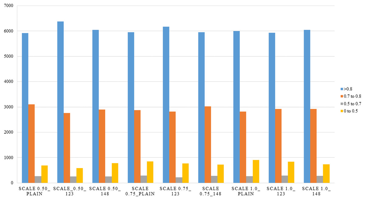
Figure 5: Overall distribution of various mean IoU ranges for the various semantic weights and scales considered.
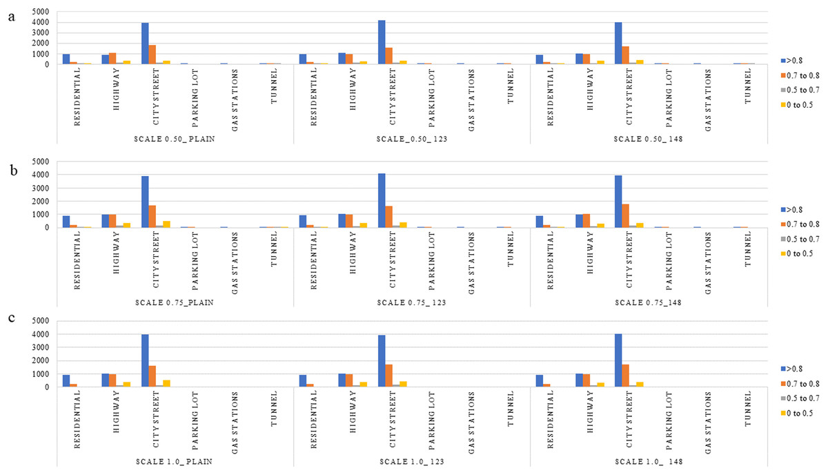
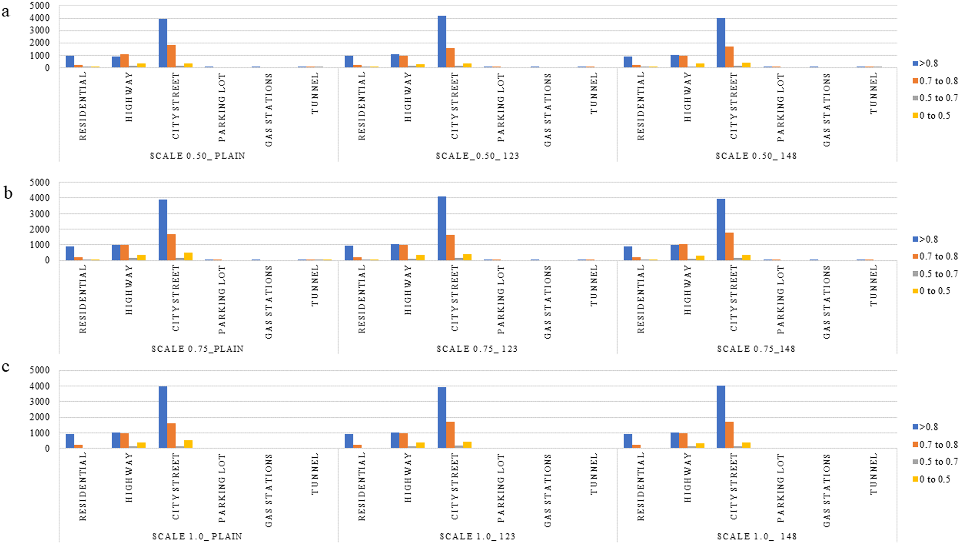
Figure 6: (A–C) Distribution of various mIoU ranges for the various semantic weights and scales considered in the context of scene type.
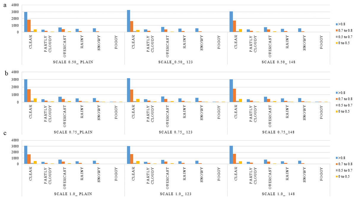
Figure 7: (A–C) Distribution of various mIoU ranges for the various semantic weights and scales considered in the context of weather.
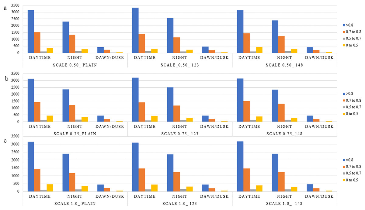
Figure 8: (A–C) Distribution of various mIoU ranges for the various semantic weights and scales considered in the context of time of day.
Furthermore, the positive impact of increased scale can be attributed to the nature of the objects being segmented. Lane markings, like most visual entities in a driving environment, are susceptible to variations in apparent size and shape due to changes in camera viewpoint and perspective distortion. These scale-induced variations are highly context-sensitive and can significantly influence the effectiveness of segmentation models. Consequently, using larger input resolutions allows the network to generalize better across diverse viewpoints by capturing lane boundaries more precisely. It is also worth noting that the LER classes in this dataset represent relatively large and geometrically simple regions compared to segmentation tasks involving densely cluttered indoor environments, where objects are small, numerous, and more intricate in form. This inherent difference in complexity makes LER segmentation less sensitive to fine-grained scaling variations, further explaining the observed performance saturation at higher scales.
In the context of semantic weighting, several important observations can be made. The vanilla configuration, which does not incorporate semantic weighting, serves as a baseline for performance comparison across all scales. Introducing semantic weights such as (1, 2, 3) yields modest improvements over the vanilla setup across almost all scales presented. This suggests that even a basic weighting strategy helps the model to better account for class imbalances.
Among the evaluated configurations, the semantic weight setting of (1, 4, 8) demonstrates the most significant overall improvement. It produces the most robust confusion matrices, effectively balancing true positive rates and reducing false positives across all classes. This weighting scheme assigns stronger penalties to the misclassification of underrepresented or more challenging classes, which encourages the model to focus on learning harder distinctions—particularly those between the L and R classes. The influence of semantic weighting is evident regardless of the specific weight values chosen. Both (1, 2, 3) and (1, 4, 8) configurations consistently outperform the baseline (unweighted) model, highlighting the general efficacy of incorporating class-based importance during training. These can be observed in the p-values presented in Table 4, especially for the metrics related to segmentation, where the lower p-values indicate a significant improvement in the performance. However, the (1, 4, 8) configuration consistently outperforms both the plain and mildly weighted variants, reinforcing the notion that applying larger penalties to challenging classes significantly reduces misclassification errors.
Moreover, the benefits of semantic weighting become even more pronounced at higher resolutions, such as scale 1.0. At this scale, the model can leverage detailed spatial features in conjunction with class importance, resulting in more accurate segmentation. This synergy allows for better recognition and separation of the most critical classes—specifically the L and R lane markings, which are vital for autonomous driving. While the (1, 2, 3) weights offer a balanced approach to learning across all classes and demonstrate improvements over the vanilla model, their advantages are more limited in scope. In contrast, the (1, 4, 8) configuration achieves superior performance in nearly all key metrics, including Pixel Accuracy, Mean Accuracy, Mean IoU, and Weighted IoU, across every scale tested. These results clearly illustrate that semantic weighting, particularly with higher class-specific penalties, is highly effective in guiding the model toward more accurate and meaningful segmentation, especially for difficult or critical classes.
These findings are consistent with the underlying hypothesis that the combination of Online Hard Example Mining (OHEM) loss and semantic weighting enhances the model’s ability to focus on more challenging and visually ambiguous samples. OHEM selectively prioritizes difficult examples during backpropagation, and when augmented with semantic weights, this effect is amplified. This dual strategy aids in better distinguishing underrepresented or visually complex classes—most notably the left (L) and right (R) lane segments, which are inherently difficult to classify due to their dependence on ego-lane-relative positioning.
Although the semantic weighting configuration of (1, 4, 8) consistently yields superior performance across metrics, some trade-offs are evident. At lower input scales, such as 0.5, this configuration shows marked gains in accuracy and recall; however, the aggressive weighting may lead to overfitting on noise or minor artifacts, particularly in regions with low spatial detail. In contrast, at higher input scales, such as 1.0, the combination of rich spatial information and targeted loss weighting results in a more balanced and robust model performance. The use of semantic weights in architectures that incorporate multi-scale receptive fields, like PPLiteSeg-STDC2, should be treated as a tunable hyperparameter. Optimal performance is achieved when the scale and weights are carefully calibrated to the task and dataset characteristics. In this study, the configuration of scale 1.0 with semantic weights (1, 4, 8) emerged as the most effective, offering improved classification precision and accuracy—especially for the L and R classes, which require spatial and directional context for accurate labelling.
It is also crucial to emphasize that the selection of semantic weight configurations should be contextually tailored to the specific requirements of the segmentation task. While the (1, 4, 8) weighting scheme has demonstrated strong performance in segmenting larger, well-structured regions such as the LER lane classes, it may not be as effective for tasks that involve finer-grained, highly detailed segmentation, where more subtle class distinctions are necessary. In such cases, a more nuanced or balanced weighting strategy may be required to avoid biasing the model toward dominant classes and to promote equitable learning across all categories.
The qualitative results illustrated in Fig. 9 further support these observations. When the same input images are subjected to segmentation under different scale and semantic weight configurations, noticeable variations in output quality are observed. These visual differences correspond closely with the trends highlighted in the quantitative metrics presented in Table 2. Specifically, images (b, e, h) and (f, g) serve as representative examples where segmentation performance varies in response to changes in scale and class weighting. These examples reinforce the conclusion that optimal segmentation performance is achieved through careful calibration of both input scale and semantic weighting—tailored to the characteristics of the target application.
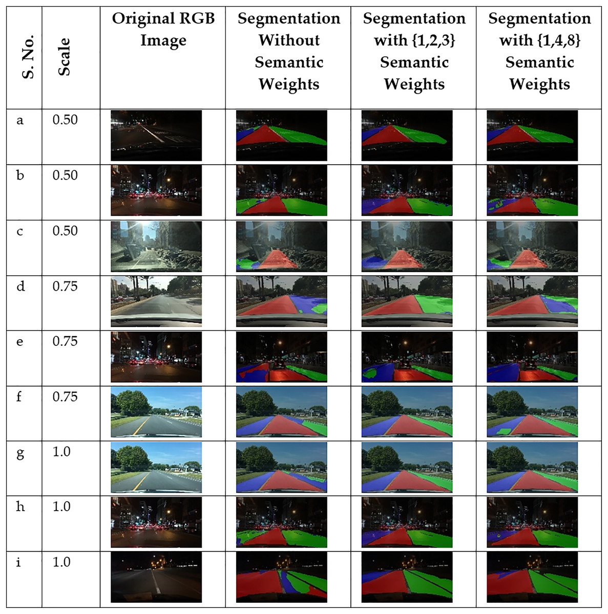
Figure 9: Results of LER segmentation overlays on RGB images.
Copyright: The Regents of the University of California.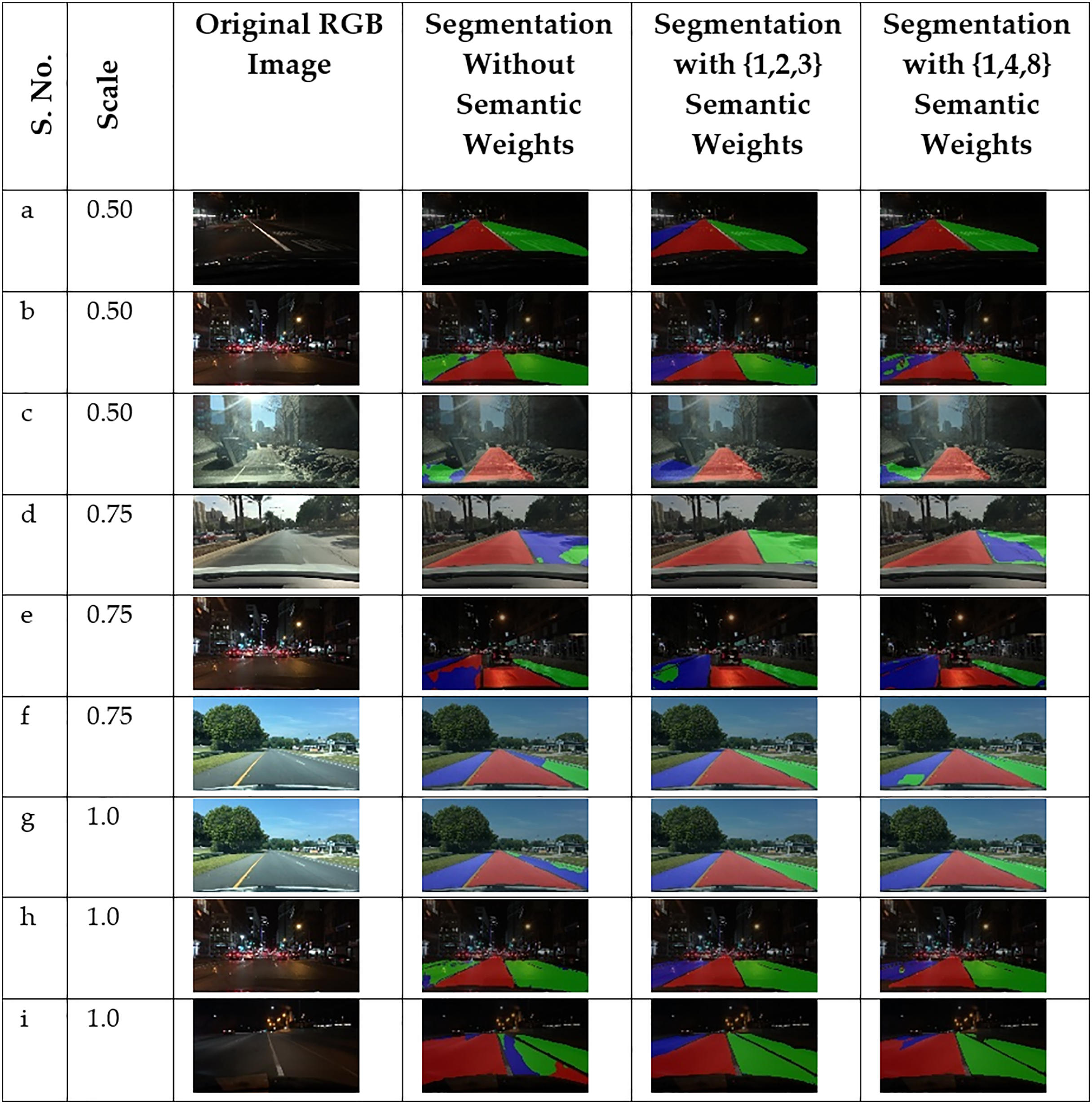
Another commonly observed issue, which is generalizable across various computer vision tasks, is the model’s reduced performance on images captured under nighttime conditions. This degradation aligns with broader trends in the field, where models tend to underperform in low-light environments compared to well-lit, daytime scenarios. The primary reason for this is the diminished availability of distinguishable visual features in nighttime imagery, which limits the model’s ability to effectively extract meaningful patterns and representations during training and inference.
Figure 10 presents sample visualizations demonstrating the complete process of embedding lane semantics into a generic Visual Perception System (VPS). These examples are extracted from a discrete set of frames within a video sequence and illustrate how lane-level segmentation is integrated across varying visual conditions. The degradation in segmentation quality under low-light conditions is evident in some of the night-time frames, further emphasizing the challenges posed by poor illumination in real-world driving environments.
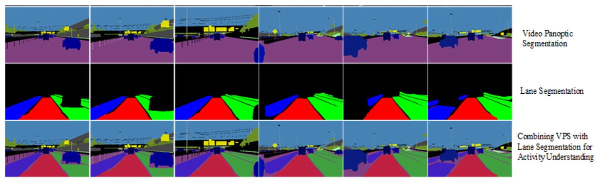
Figure 10: Results of lane-semantic inclusive VPS.
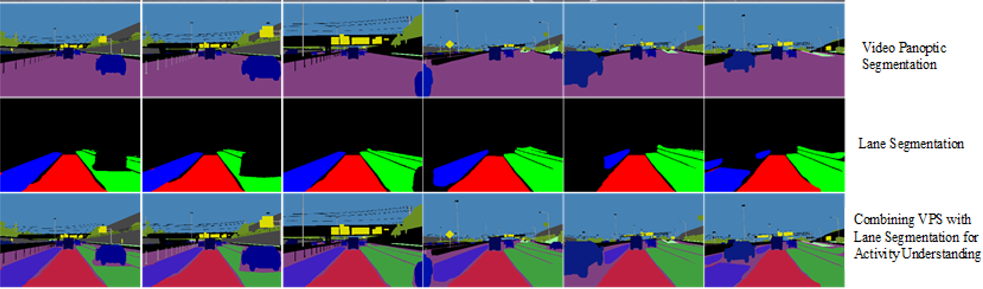
Discussion
The results of this study demonstrate the significant impact of semantic weighting and input scale on the performance of lane segmentation models, particularly in the context of autonomous driving. Our findings highlight the effectiveness of the PPLiteSeg-STDC2 network, which benefits from both larger input scales and the use of semantic weights, as these strategies allow the model to better distinguish challenging classes such as the left (L) and right (R) lanes. This observation aligns with previous studies, such as Zou et al. (2019), which showed the positive influence of larger input scales in improving the segmentation of complex lane structures, where finer details are crucial for accurate classification.
The introduction of semantic weights, particularly the configuration of (1, 4, 8), was found to significantly outperform the baseline (vanilla) model. This outcome supports findings from Badrinarayanan, Kendall & Cipolla (2017) and Li, Li & Zhuang (2020), where incorporating class-specific penalties led to a reduction in misclassification errors, especially for L and R classes, which must not be misclassified. Moreover, we observed diminishing returns with further increases in semantic weight, a trend consistent with studies in similar domains, such as Chen et al. (2018), where larger penalties did not correspond to proportional improvements, especially when model overfitting became a concern. Specifically, at lower scales, the (1, 4, 8) configuration showed strong gains, but at the 1.0 scale, the performance became more balanced and robust, reflecting the diminishing effect of higher weights at richer resolutions.
A key takeaway from our findings is the importance of tuning both semantic weights and input scales according to the task’s specific needs. While the (1, 4, 8) configuration was optimal for the broader, less intricate lane segmentation task, tasks requiring finer segmentation of smaller regions may benefit from a different set of weights. This aligns with previous literature, which suggested that optimal hyperparameter configurations are highly task dependent. Further, the performance at scale 1.0 with semantic weights (1, 4, 8) reflects the balance of spatial resolution and class emphasis. This has been shown to improve segmentation accuracy, especially for classes, as misclassifications could lead to undesirable outcomes in the application’s context, in other related work (Liu et al., 2018).
Another common challenge noted in our study, consistent with the findings (Wang, Ren & Qiu, 2018), is the poor performance of the model under night-time or low-light conditions. This issue, widespread across computer vision tasks, is primarily attributed to the scarcity of visual features under low illumination, which hampers the model’s ability to learn and generalize effectively. Previous research (Ren et al., 2019) also reported a similar degradation in segmentation accuracy under night-time conditions, suggesting that the lack of distinguishable features in images significantly impacts the model’s ability to perform robustly. Addressing this limitation remains an ongoing challenge in the field, and potential solutions, such as domain adaptation or low-light enhancement techniques (Li et al., 2021), could be explored in future work.
Conclusions
This work presents a novel approach to the Visual Panoptic Segmentation (VPS) task, addressing the lane class segmentation, which can be incorporated into the VPS. By leveraging state-of-the-art networks for tracking and segmentation of things and segmentation of stuffs, generalization capabilities are demonstrated with a higher level of lane semantics incorporated into the VPS task. This approach eliminates the need for joint learning and the labor-intensive task of annotating extensive VPS datasets, thus offering a more efficient solution and reducing dependency on specialized datasets. The proposed framework provides flexibility in choosing high-performance networks for individual tasks, improving the performance of each task independently. This flexibility is especially beneficial in enhancing scene understanding for autonomous driving applications, such as the incorporation of drivable area segmentation within the VPS. A key innovation of our approach is the introduction of semantic weights during training, which significantly improves the model’s ability to avoid misclassification—particularly critical in tasks where precision is paramount, such as lane marking segmentation and classification.
The results from our experiments clearly demonstrate the superior performance of networks trained with semantic weights, highlighting their effectiveness in reducing misclassification errors. Furthermore, our study confirms that combining larger input scales with semantic weighting enhances the accuracy of lane segmentation models for autonomous driving. However, challenges remain, particularly in handling lower scales and low-light conditions, which affect model robustness. Though the method of using semantic weights has proven to work well for the LER segmentation. The choice of the weights seems to be a heuristic and hence becomes a tunable parameter. This might prove to be a limitation. These findings suggest the importance of continuing to refine semantic weighting strategies and exploring solutions for nighttime segmentation. Future research should focus on advancing these strategies, potentially incorporating multi-modal data or leveraging advanced image enhancement techniques to improve performance under diverse environmental conditions.