
Steel surface defect detection based on multi-scale dynamic convolution and lightweight cross-stage fusion
- Published
- Accepted
- Received
- Academic Editor
- Consolato Sergi
- Subject Areas
- Artificial Intelligence, Computer Vision, Neural Networks
- Keywords
- Steel surface defect detection, Object detection, Multi-scale dynamic convolution, Feature extraction, Cross-stage fusion
- Copyright
- © 2026 Zhang et al.
- Licence
- This is an open access article distributed under the terms of the Creative Commons Attribution License, which permits unrestricted use, distribution, reproduction and adaptation in any medium and for any purpose provided that it is properly attributed. For attribution, the original author(s), title, publication source (PeerJ Computer Science) and either DOI or URL of the article must be cited.
- Cite this article
- 2026. Steel surface defect detection based on multi-scale dynamic convolution and lightweight cross-stage fusion. PeerJ Computer Science 12:e3485 https://doi.org/10.7717/peerj-cs.3485
Abstract
To address the primary challenges of inadequate multi-scale defect perception capabilities and limited computational resources on edge devices in steel surface defect detection scenarios, this article proposes a steel surface defect detection based on multi-scale dynamic convolution and lightweight cross-stage fusion (LightSDD). First, to adaptively enhance the feature representation ability of small targets, the multi-scale dynamic convolution kernel is fused with the channel attention mechanism, and a fine-grained feature fusion method based on C3k2 multi-scale dynamic convolution is proposed. Next, to reduce redundant parameters while retaining key positioning information, an interpolation alignment strategy is adopted for multi-resolution features, along with channel compression and cross-resolution feature concatenation, based on the replacement of the original you only look once version 11 (YOLOV11) detection head. This approach enables the design of a lightweight cross-stage detection head, LSCD. Later, comparative experiments on the NEU-DET and GC10-DET datasets demonstrate that LightSDD outperforms seven state-of-the-art methods. Finally, performance tests on edge devices indicate that LightSDD exhibits strong robustness and practicality. Code is available at: https://github.com/chaoszzz-zyx/LightSDD (DOI: 10.5281/zenodo.17012588).
Introduction
In automotive manufacturing, shipbuilding, aerospace, and precision machinery, steel plates with surface defects—such as pits, inclusions, indentations, or rough patches—compromise the material’s corrosion resistance, wear resistance, and fatigue strength, potentially leading to structural failure and posing significant safety risks. The current detection methods include manual inspection, machine learning (Malhotra, 2015), and deep learning (He et al., 2019), among others. The manual inspection method relies on visual inspection, which is difficult to meet the requirements of real-time online inspection on high-speed rolling lines. Detection methods based on machine learning, such as support vector machines and decision trees, are often limited by the design of artificial features and have relatively weak generalization capabilities.
Deep learning-based object detection algorithms are broadly categorized into two-stage and one-stage methods. The fundamental principle of the two-stage approach is to decompose the detection process into two sequential steps: first, generating region proposals, and then performing classification and boundary regression on these proposals. The representative models include regions with convolutional neural network (R-CNN) (Girshick et al., 2014), Fast R-CNN (Choi & Han, 2024), Faster R-CNN (Xu et al., 2022), Mask R-CNN (Wang, Li & Wan, 2022), Cascade R-CNN (Wang et al., 2024), etc. For example, Girshick et al. (2014) pioneered the application of CNNs in object detection by generating candidate regions through Selective Search and independently extracting CNN features, thereby laying the foundation for deep learning methods, albeit with low efficiency. Choi & Han (2024) used the Fast R-CNN to classify the surface condition of rails and predict internal rail defects. Fast R-CNN proposes sharing convolutional feature maps with the region of interest (ROI) pooling layer to achieve unified feature extraction for candidate regions, and integrating classification and regression into a single network for end-to-end training. However, the generation of candidate regions remains an independent and slow module, and the detection process has a speed bottleneck. Xu et al. (2022) proposed a steel surface defect detection model based on the improved Faster R-CNN. In this method, the ResNet50 is replaced with the RegNet. The transformer spatial attention mechanism is adopted to enable the network to more accurately focus on the target area. Moreover, through transfer learning, multi-scale training, and cosine annealing learning rate adjustment strategies, the detection accuracy is improved. Wang, Li & Wan (2022) proposed a new type of track surface defect detection network based on Mask R-CNN. This network introduces a dual fusion path to achieve deep integration of feature maps at each stage, and adopts a new evaluation metric, complete intersection over union (CIOU), which, to some extent, achieves a balance between accuracy and speed, but still lags behind other single-stage object detection models. Wang et al. (2024) developed a method based on the improved Cascade R-CNN. This approach utilizes residual network (ResNet) and path aggregation feature pyramid network (PAFPN) as the feature extraction network, replaces ROI pooling with ROI Align, and employs bicubic interpolation instead of bilinear interpolation, thereby addressing the issue of detecting metal surface defects in blurry backgrounds. Overall, the two-stage detection algorithm exhibits good detection accuracy; however, its complex cascading structure and excessive computational redundancy lead to low deployment efficiency.
End-to-end one-stage object detection combines object positioning and classification into a single-stage detection architecture. The core idea is to eliminate the time-consuming step of candidate region generation and directly predict the class probabilities and bounding box coordinates of all objects in the input image through dense sampling or preset anchor points at once. Typical methods include single-shot detector (SSD) (Liu & Gao, 2021), the You Only Look Once (YOLO) series (Xie, Sun & Ma, 2024; Huang, Zhu & Huo, 2024; Lu et al., 2024; Ma et al., 2025; Zhao et al., 2024; Luo et al., 2025; Xie, Ma & Sun, 2025), RetinaNet (Akhyar et al., 2019), MirageNet (Fu et al., 2025), and MobileNet (Fu et al., 2024), etc. Liu & Gao (2021) optimize the ResNet50 backbone network by applying knowledge distillation techniques, employs a feature fusion strategy to enhance the detection capability for small-sized defects, and utilizes a channel attention mechanism to reduce computational resource consumption. Xie, Sun & Ma (2024) design a lightweight multi-scale feature fusion module called C2f_LMSMC, which integrates the EGAM attention mechanism and stacked convolution operations to facilitate feature interaction across different dimensions, thereby effectively improving the recognition accuracy of small defects. Huang, Zhu & Huo (2024) proposed the SSA-YOLO model, which integrated the Swin Transformer and the Adaptive Spatial Feature Fusion technology into YOLOv5. This model significantly improves the detection of the most difficult crack defects on the NEU-DET dataset. In response to the problem of insufficient robustness in existing methods for complex defect shapes, Lu et al. (2024) proposed the improved YOLOv8 network, WSS-YOLO. This method introduces the WIoU loss function and the C2f-DSC dynamic snake convolution module, enabling the model to adaptively adjust its receptive field and provide a new technical approach for real-time defect detection in industrial sites. Ma et al. (2025) proposed ELA-YOLO, which introduced a linear attention mechanism into the network. This mechanism helps control computational complexity while enhancing the model’s representational ability, enabling the precise identification of multi-scale surface defects under limited computing resources. In response to the problem that steel surface defects in complex industrial environments are easily interfered with by light, texture, and noise, and are difficult to detect in real time and accurately, Zhao et al. (2024) proposed a lightweight network MSAF-YOLOv8n based on YOLOv8n. This method enhances the model’s feature fusion ability by introducing the multi-scale adaptive fusion module MS-AFB and the dynamic coordinate attention-enhanced Dynamic Coordinate Attention Ghostconv Space Pooling Pyramid-fast Cross-stage Partial Convolutional (DCA-GSPPFCSPC) structure. Regarding the issue of tiny surface defects on steel bridge welds, Luo et al. (2025) proposed a lightweight network called SFW-YOLO based on YOLOv8s. This method captures fine-grained features through the introduction of the high-resolution P2 layer and constructs the DyHead dynamic detection head to enhance multi-scale attention. It optimizes detection accuracy in the presence of multi-scale defects and complex backgrounds, while also improving the ability to identify small-sized defects. Xie, Ma & Sun (2025) made contributions to resolving the trade-off issue between lightweight and multi-scale feature fusion in existing steel surface defect detection networks by introducing the lightweight multi-scale module LighterMSMC, the re-parameterized feature fusion pyramid DE-FPN, and the group convolution Efficient Head. To address the issues of tiny defects on steel surfaces and the imbalance of defect categories, Akhyar et al. (2019) proposed an upgraded RetinaNet defect detection module. Its feature pyramid network and anchor point strategy enhance the accuracy, but at a higher cost. Fu et al. (2025) achieved a significant reduction in computational complexity while maintaining high accuracy through dynamic sparse convolution technology and a hierarchical feature reuse mechanism. This method employs hardware-friendly sparse operators and neural architecture search for edge devices to achieve a substantial reduction in Floating Point Operations (FLOPs). Later, Fu et al. (2024) proposed an improved method, where the proposed frequency recalibration module combined frequency domain analysis with channel attention for the first time; the designed cascaded dilated convolution pyramid maintained the receptive field coverage of multi-scale lesions while reducing FLOPs. Zhao et al. (2024) propose a lightweight MSAF-YOLOv8n algorithm. By introducing a multi-scale adaptive fusion module and reconstructing the detection head, the method significantly reduces model parameters and computational load while achieving high-precision, real-time detection of steel surface defects in complex backgrounds. Yang & Liu (2024) design cross-stage partial FasterNet blocks to enhance multi-scale feature extraction and reduce computational overhead. They construct an adaptive fusion spatial pyramid pooling module to expand the receptive field and improve the decoupled detection head, thereby balancing classification and regression tasks. These contributions ultimately form CAT-YOLO, a high-precision lightweight model for real-time steel defect detection. Liu et al. (2025) address the challenges of unstructured and multi-scale characteristics in steel surface defects by developing GC-Net based on YOLOv8. The framework incorporates a global attention module to enhance modeling capability for unstructured defects, and designs a cascaded fusion network to handle multi-scale defect problems. This effectively improves the model’s ability to capture global information and fuse multi-scale features. One-stage detection algorithms simplify the training process, offer fast detection speed, and are easy to deploy, making them a commonly adopted solution for steel defect detection. However, they still suffer from issues such as potentially missing small targets and having relatively low positioning accuracy.
Overall, the detection of surface defects in steel still faces two main challenges: (1) Static calculation models are difficult to adapt to different complexity scenarios. In simple scenarios, there is computational redundancy, while in complex scenarios, the detection capability is insufficient. (2) The contradiction between shallow features, which are rich in detail but weak in semantic abstraction, and deep features, which are semantically rich but suffer from relatively low positioning accuracy, limits the detection precision for subtle defects on steel surfaces. Existing studies predominantly focus on either feature extraction or lightweight optimization, yet fail to simultaneously address the dual requirements of multi-scale dynamic perception and computational constraints on edge devices. To bridge this gap, this article proposes the LightSDD algorithm, which aims to achieve synergistic optimization of detection accuracy and real-time performance through a dynamic kernel adaptation mechanism and a lightweight cross-stage fusion architecture.
To address the limitations of existing research in multi-scale dynamic perception and efficient edge inference, the main contributions of this article are as follows:
-
(1)
We presented LightSDD, a lightweight surface defect detection algorithm designed for deployment on edge devices, which enhances the detection accuracy and recall of multi-scale fine defects on steel surfaces. This method provides a novel solution for real-time, high-precision detection in resource-constrained industrial edge computing environments.
-
(2)
A fine-grained feature fusion method based on C3k2 multi-scale dynamic convolution was proposed. This method dynamically generates multi-scale convolution kernel weights through the C3k2_PKI dynamic convolution module combined with the channel attention mechanism, enabling adaptive enhancement of features for small targets and complex-shaped defects.
-
(3)
A lightweight cross-stage detection head, LSCD, was designed. LSCD optimizes inference efficiency through a dynamic parameter regulation mechanism and maintains positioning accuracy by combining channel compression and cross-resolution fusion with spatial attention, resulting in a 6.20% reduction in parameters.
-
(4)
Experimental results on the NEU-DET and GC10-DET datasets show that the proposed LightSDD has achieved excellent performance in detecting several fine surface defects of steel, such as patches, waist folding, and silk spots.
The remainder is as follows. ‘Methods’ provides a detailed description of the algorithm proposed in this article. ‘Performance Test Results and Analysis’ presents ablation studies, comparative experimental results and analysis, along with performance tests on edge devices. ‘Discussion’ is the discussion section. ‘Conclusion’ is the summary section.
Methods
Overview
This section proposes steel surface defect detection based on multi-scale dynamic convolution and lightweight cross-stage fusion (LightSDD). Figure 1 illustrates the LightSDD network architecture. Firstly, the C3k2_PKI (Khanam & Hussain, 2024), which is built upon dynamic multi-scale perception, is meticulously designed to construct a multi-level feature pyramid network. Shallow high-resolution features (1/8 scale) are adept at retaining detailed textures. Middle-level features (1/16 scale) strike a balance between semantics and positioning accuracy. Deep low-resolution features (1/32 scale) focus on capturing global context. The module effectively facilitates adaptive matching of cross-scale receptive fields by integrating multi-scale convolutional kernels (Qi & Jing, 2022) (varying from 3 × 3 to 11 × 11) with a dynamic weight fusion mechanism. This, in turn, enhances the model’s generalization capabilities in addressing defects of diverse dimensions. Subsequently, the YOLOv11 detection head undergoes substitution with the LSCD head. This head innovatively adopts channel compression (Cheng et al., 2021) and cross-stage fusion (Wang et al., 2024) strategies. These strategies reduce parameters and elevate positioning accuracy, catering to the stringent robustness demands inherent in industrial quality inspection scenarios. Finally, these two components are integrated into the YOLOv11 framework to form the end-to-end LightSDD architecture, achieving an optimal balance between multi-granularity feature representation and computational efficiency. The pseudocode of the LightSDD is presented in Algorithm 1.
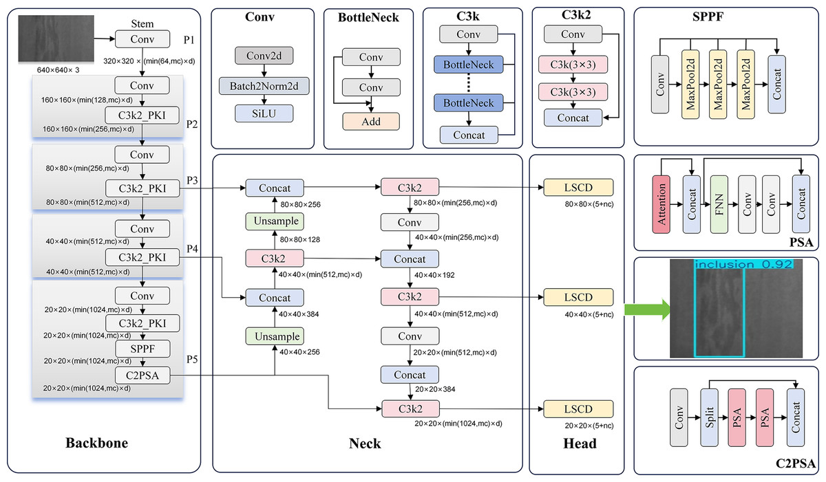
Figure 1: LightSDD network architecture.
The end-to-end structure of the LightSDD, which consists of the backbone network, the C3k2_PKI dynamic convolution module, and the LSCD lightweight detection head. The input image undergoes multi-scale feature extraction through the backbone and is then passed to the C3k2_PKI module for dynamic weight fusion, enhancing multi-scale defect perception capability. Subsequently, the LSCD detection head performs cross-stage feature alignment, channel compression, and fusion, ultimately outputting defect classification and localization results.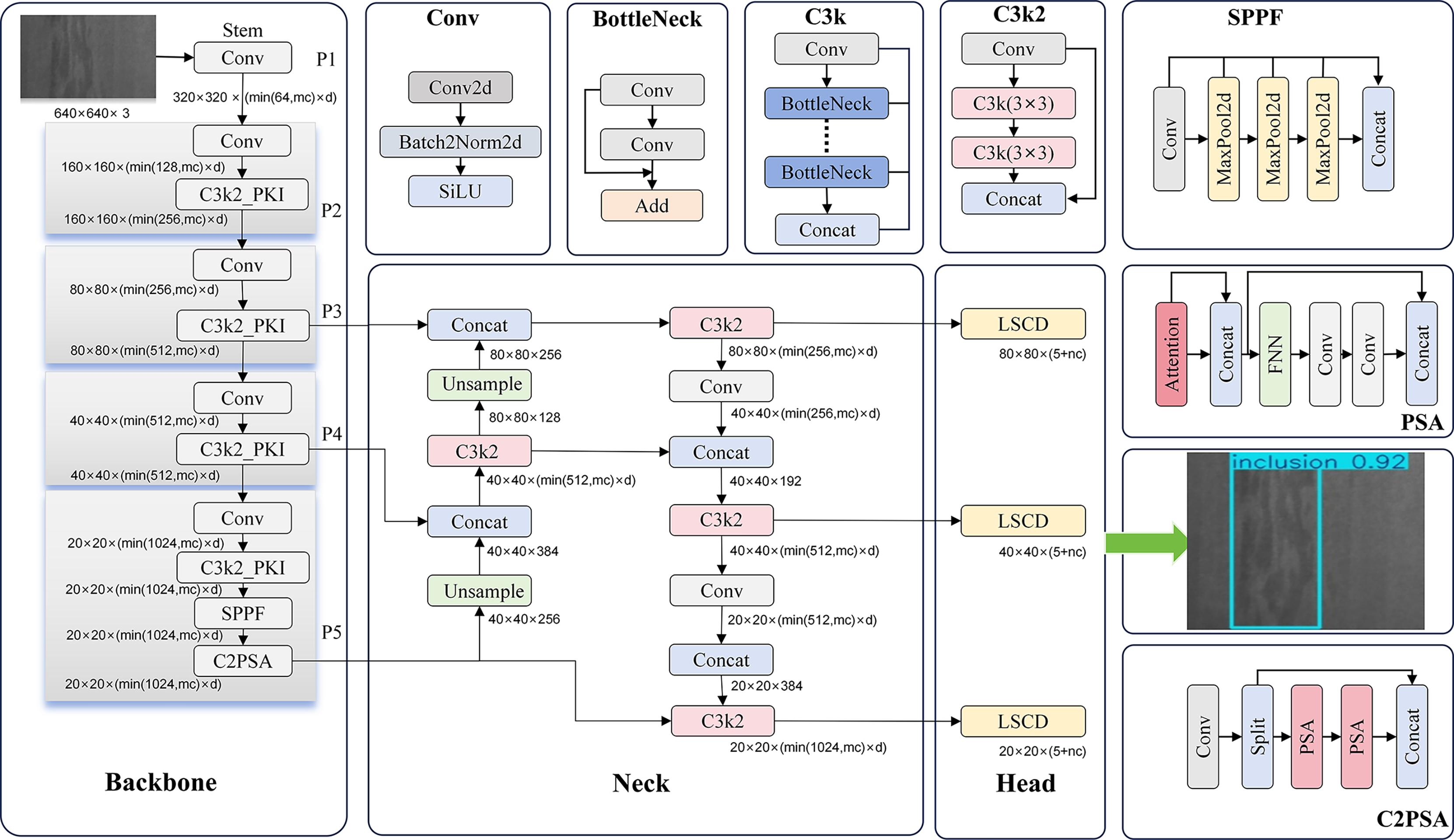
| Input:NEU-DET steel defect images |
| Output:Defect detection results (bounding box, class, confidence) |
| 1 # ------------------- Backbone feature extraction ------------------------------- |
| 2 # extract multi-scale features (P3: , P4: , P5: ) |
| 3 , , = LightSDD_Backbone(x) |
| 4 # ------------ Dynamic convolution optimization module(C3k2_PKI) -------------------- |
| 5 for s in [P3, P4, P5]: |
| 6 # multi-scale dynamic convolution kernel parallel feature extraction (Eq. (1)) |
| 7 = Conv( , kernal = k in [3, 5, 7, 9, 11], stride = 1, padding = k/2) |
| 8 # generate dynamic weights (calculation of in Eq. (4)) |
| 9 = SE_Block(GAP( )) |
| 10 # weighted fusion (Eq. (5)) |
| 11 = Sum( * ) |
| 12 # ------------------- Lightweight cross-stage detection head (LSCD) -------------------- |
| 13 # cross-resolution alignment & channel compression (Eq. (11)) |
| 14 = Bilinear_Interpolate( , size= ) |
| 15 = Bilinear_Interpolate( , size= ) |
| 16 = ( , ) |
| 17 = ( , ) |
| 18 # cross-stage feature concatenation & interaction (Eqs. (12), (13)) |
| 19 = Concat( , , ) # cross-stage feature concatenation |
| 20 = Light_Transformer( , heads = 4) # lightweight transformer for long-range dependencies |
| 21 # group convolution & dynamic channel recalibration (Eqs. (14), (15)) |
| 22 Ffused = ( , groups = 8) # group convolution |
| 23 = SE_Block( ) # dynamic channel recalibration |
| 24 # ------------------- Dynamic parameter adjustment (Edge Optimization)------------------- |
| 25 if edge_inference: |
| 26 # dynamic kernel downgrade (Eq. (10)) |
| 27 if latency > threshold: replace_kernel(11 × 11→7 × 7) |
| 28 # channel pruning (Eqs. (17), (18)) |
| 29 prune_channels(gradient < μ) # remove low-gradient channels |
| 30 # output detection results |
| 31 bbox_pred, cls_pred = Detection_Layer( ) |
| 32 return bbox_pred, cls_pred |
In Algorithm 1, Step 3 involves the backbone feature extraction stage. Here, the input is an industrial quality inspection image ( ). The backbone network extracts multi-scale features , and . In this context, H and W represent the height and width of the original image, and C denotes the feature dimension. , and correspond to shallow high-resolution, middle mid-resolution, and deep low-resolution features, respectively.
Steps 5–11 form the dynamic convolution optimization module. To perform parallel multi-scale kernel extraction on the features, (s ∈ {P3, P4, P5}) from the previous layer, 3 × 3, 5 × 5, 7 × 7, 9 × 9, and 11 × 11 convolution kernels are applied to generate multi-branch features . Subsequently, the squeeze-and-excitation (SE) module produces branch weights, = [ , , , , ], and a weighted summation is performed to achieve dynamic weight fusion, updating the features of the current scale.
Steps 14–17 describe the lightweight cross-stage detection head. First, and are upsampled via bilinear interpolation to align their resolutions of , yielding and . Subsequently, A 1 × 1 convolution is then used to compress the channels of the upsampled features, unifying them to 256 dimensions, resulting in and .
Steps 19–23 focus on feature fusion and enhancement. Initially, the , and are concatenated to generate fused features ( ). Subsequently, a lightweight transformer is employed to model long-range dependencies, thereby producing enhanced features ( ). The process utilizes group convolution ( ) to compress through channel grouping. Finally, dynamic channel recalibration is performed using an SE module, resulting in the final features ( ).
Steps 25–29 address dynamic parameter adjustment. Specifically, if the model operates on edge devices and the average forward inference latency exceeds the predefined threshold, the 11 × 11 kernel is downgraded to a 7 × 7 kernel. Additionally, low-sensitivity channels are pruned based on gradient sensitivity analysis (Wang et al., 2018) to minimize computational overhead.
Steps 31–32 outline the model output stage. In this stage, the detection layer predicts the final feature ( ) to generate bounding box predictions (bbox_pred) and class predictions (cls_pred).
C3k2 poly kernel inceptional design
1) Fine-grained feature fusion via multi-scale dynamic convolution. The C3k2 poly kernel inceptional (C3k2_PKI) incorporates the idea of multi-scale convolutional kernels, performing fine-grained convolution operations on different scales of the input image to extract rich feature representations. Given an input feature map, (s {P3, P4, P5}), the module initially applies parallel multi-scale convolutions, as shown in Eq. (1).
(1) where, denotes a convolutional kernel, where each convolutional branch captures both local structural and global semantic information at its corresponding scale.
After obtaining multi-scale features, the method designs a dynamic weight computation mechanism to avoid information redundancy caused by simple concatenation or summation operations. It introduces a lightweight attention module (Wu et al., 2025) to generate adaptive weights. First, global average pooling (GAP) (Jin et al., 2022) aggregates the output of each scale branch, as shown in Eq. (2).
(2) where, and represent the height and width of the feature maps at different levels.
Next, a series of fully connected layers (Basha et al., 2020) and nonlinear activation functions (Hsiao et al., 2019) transform these statistics to generate corresponding weight vectors, where denotes the ReLU activation function, as shown in Eq. (3).
(3)
Subsequently, the softmax function normalizes the weights of each branch to ensure learnable and dynamically adjusted contribution ratios across multi-scale features, as shown in Eq. (4).
(4) where, are fully connected layer weights of the SE module, denotes the bias of the channel attention intermediate layer, and corresponds to the bias of the channel attention output layer, satisfying .
Finally, the method performs weighted summation on multi-scale features according to their corresponding weights, producing refined fused features, as formulated in Eq. (5).
(5) This method enables cross-resolution feature interaction (Lu et al., 2025) and enhances small-object sensitivity, effectively allowing the model to learn objects at various scales.
2) Dynamic parameter control mechanism. First, the input feature analysis performs global average pooling on the multi-scale feature maps (P3, P4, P5) output by the backbone, generating channel descriptor vectors as shown in Eq. (6), where denotes the number of channels.
(6)
The scale-specific descriptor vectors are subsequently concatenated to form a unified multi-scale feature representation, as formulated in Eq. (7).
(7)
This vector is fed into a two-layer fully connected network multilayer perceptron (MLP, with hidden layer dimension ), outputting a score vector Sk = [ ], representing the saliency scores for small, medium, and large targets, respectively. As shown in Eq. (8):
(8) where, denotes the weight matrix of the MLP hidden layer, represents the weight matrix of the MLP output layer, is the bias term of the global feature hidden layer, and is the bias term of the importance score output layer.
Finally, the scores undergo normalization via the softmax function to constrain their distribution, as shown in Eq. (9):
(9) where, , , represent the importance weights for small, medium, and large targets, satisfying .
The parameter dynamic adjustment adaptively selects convolution kernel sizes and computational intensity based on the importance weights and the real-time workload. If the inference latency exceeds a threshold, the 11 × 11 kernel is automatically replaced with a 7 × 7 kernel, as shown in Eq. (10):
(10) The structure of the C3k2_PKI is illustrated in Fig. 2.

Figure 2: Structure of C3k2_PKI.
This module employs multi-branch parallel convolutions to extract multi-scale features. Each branch is followed by an SE attention mechanism that generates dynamic weights, which are then used for weighted fusion to produce enhanced features.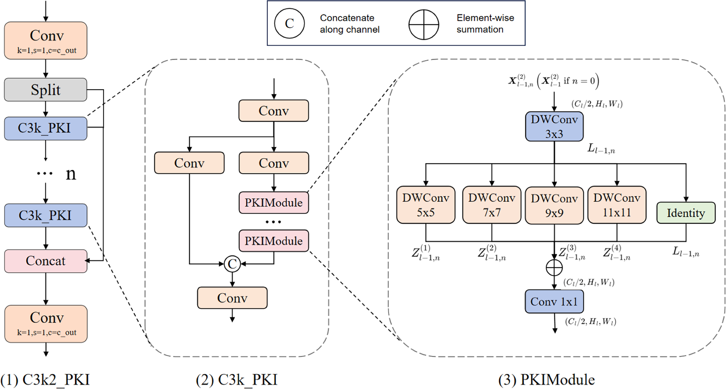
Lightweight shared convolutional detection head design
1) Cross-stage feature fusion. First, the feature maps P3 (1/8 scale), P4 (1/16 scale), and P5 (1/32 scale) are extracted from the backbone, with channel numbers C3 = 256, C4 = 512, and C5 = 1,024, respectively.
Then, bilinear interpolation is applied to P4 and P5 to upscale their resolution to match P3 (1/8 scale). A 1 × 1 convolution is used to compress the channels of P4 and P5 to 256, aligning them with P3, as shown in Eq. (11).
(11)
Finally, the aligned feature maps are output as , and .
The bidirectional feature interaction consists of a bottom-up path and a top-down path, which model cross-stage dependencies through a lightweight attention mechanism (Xu et al., 2025). In the bottom-up path, the P3 features are concatenated with the compressed P4 and P5 features to generate a global context vector, as shown in Eq. (12).
(12)
Long-range dependencies are modeled using a lightweight transformer encoder (four attention heads, hidden layer dimension of 128), as shown in Eq. (13).
(13)
The top-down path splits Ftrans into three components, which are then element-wise added to the original P3, P4, and P5 features, respectively, for information feedback, as formulated in Eq. (14).
(14) The channel compression and enhancement strategy retains key information by reducing redundant channels. Dimensionality reduction is performed via group convolution, where the concatenated features ∈ are compressed to 128 channels using group convolution (groups = 8), as formulated in Eq. (15).
(15)
The process employs dynamic channel recalibration through a lightweight Squeeze-and-Excitation (SE) module to adaptively adjust channel-wise weights, as formulated in Eq. (16).
(16)
2) Parameters optimization. For each output channel of each convolutional layer in the detection head, calculate the mean of the absolute values of the weight gradients, as shown in Eq. (17).
(17) Here, C represents the number of channels in the current layer, and denotes the weight gradient of the C-th channel. Channels with gradient sensitivity below the mean μ are pruned, retaining only the important ones.
Finally, channels in the LSCD detection head with gradient magnitudes below the mean are sparsified. The retention rate r is computed as shown in Eq. (18).
(18)
The structure of the used LSCD is illustrated in Fig. 3.
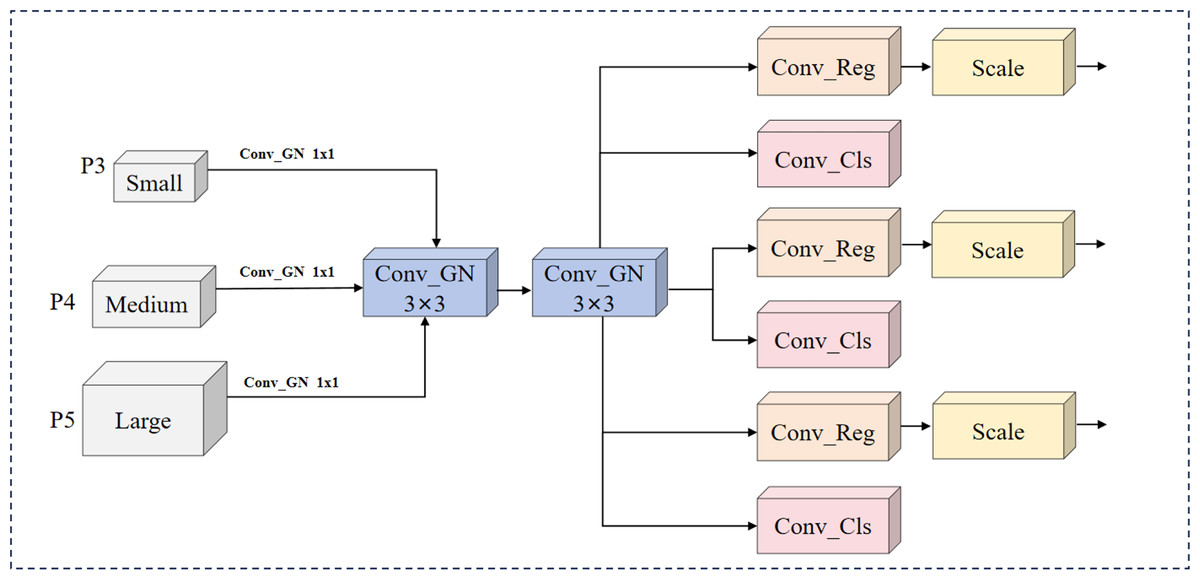
Figure 3: LSCD structure.
The LSCD head receives multi-scale features from C3k2_PKI. It first performs bilinear upsampling and channel compression on P4 and P5 to align their resolutions with P3. Subsequently, it concatenates the features and uses a lightweight Transformer to model long-range dependencies. The features then undergo group convolution and SE channel recalibration to enhance feature representation. Finally, the head outputs fused features for classification and regression.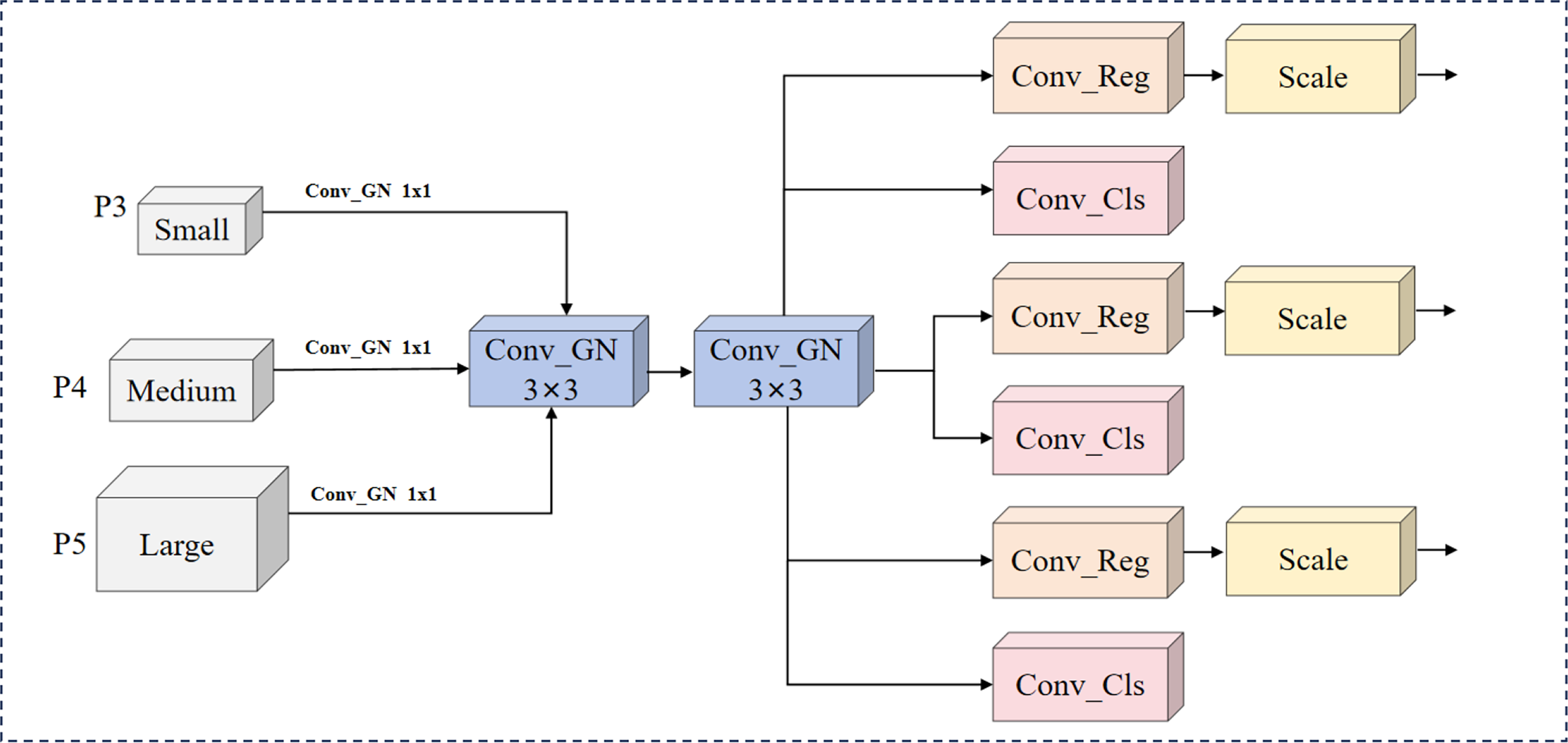
Performance test results and analysis
Experimental setup, dataset, and evaluation metrics
This study conducts experiments on the Windows 11 operating system, utilizing Python 3.10.16 and PyTorch 2.5.1 as the deep learning framework and PyCharm as the development environment. The hardware consists of an Intel Core i5-13500H CPU and an RTX 4050 GPU with 6 GB of VRAM, utilizing CUDA 12.4 for GPU acceleration. The hyperparameter configuration for training the LightSDD model is shown in Table 1.
| Hyperparameters | Settings |
|---|---|
| Image size | 640 × 640 |
| Epochs | 300 |
| Batch size | 8 |
| Mosaic | 1.0 |
| Close mosaic | 0 |
| Workers | 4 |
| Optimizer | SGD |
| Learning rate | 0.01 |
| Momentum | 0.937 |
| Weight decay | 0.0005 |
This article adopts the NEU-DET and GC10-DET datasets for testing. The NEU-DET steel defect dataset consists of six types of defects: crazing, inclusion, patches, pitted surface, rolled-in scale, and scratches, with 300 images per category, totaling 1,800 images. The GC10-DET steel surface defect dataset includes ten types of defects: punching, welding line, crescent gap, water spot, oil spot, silk spot, inclusion, rolled pit, crease, and waist folding. NEU-DET can be downloaded at http://faculty.neu.edu.cn/songkechen/zh_CN/zdylm/263270/list. GC10-DET can be downloaded at https://github.com/lvxiaoming2019/GC10-DET-Metallic-Surface-Defect-Datasets. During the experiment, a five-fold cross-validation is employed to establish training sets, test sets, and validation sets for both the NEU-DET and GC10-DET datasets, ensuring rigorous and objective verification results.
This article employs Precision, Recall, mean Average Precision (mAP), Parameters, and Floating Point Operations (FLOPs) as metrics to evaluate model performance. Specifically, mAP50 denotes the mean average Precision calculated at an Intersection over Union (IoU) threshold of 0.5, while mAP50~95 represents the average of multiple mAP values obtained at IoU thresholds ranging from 0.5 to 0.95. Parameters refer to the total count of learnable parameters that require optimization during model training. In contrast, FLOPs quantify the computational complexity of the model by measuring the total number of floating-point operations required for a single forward propagation.
Ablation study
To evaluate the performance of different modules in LightSDD, YOLOv11 is used as the baseline (denoted as S0), and an ablation study is conducted on the NEU-DET dataset using the configuration specified in Table 1. The performance metrics of the ablation experiments are summarized in Table 2.
| Algorithm | C3k2_PKI | LSCD | mAP50 (%) | mAP50~95 (%) | Parameters (M) | Significance (mAP50) | Significance (mAP95) |
|---|---|---|---|---|---|---|---|
| S0 | × | × | 78.00 ± 1.00 | 44.70 ± 1.10 | 2.58 | (Baseline) | (Baseline) |
| S1 | √ | × | 78.29 ± 0.98 | 44.35 ± 1.69 | 2.58 | p = 0.144 | p = 0.625 |
| S2 | × | √ | 78.62 ± 1.40 | 45.97 ± 1.10 | 2.42 | p = 0.159 | p = 0.043 |
| S3 (LightSDD) | √ | √ | 76.81 ± 1.25 | 44.86 ± 0.33 | 2.42 | p = 0.048 | p = 0.709 |
From the observations in Table 2:
-
(1)
The C3k2_PKI module adaptively integrates features across multiple scales, enhancing the model’s perception capability for micro-defects and complex backgrounds. As a result, S1 improves mAP50 by 0.29%. However, due to the increased computational cost from using larger convolutional kernels, mAP50~95 experiences a slight decrease of 0.35%.
-
(2)
S2 reduces parameters by 6.20%, demonstrating that the lightweight cross-stage detection head (LSCD) effectively reduces redundant parameters through channel compression and group convolution, while preserving detailed information in cross-resolution features. This optimization improves detection accuracy.
-
(3)
S3 (LightSDD) achieves more robust feature representation through collaborative optimization while maintaining parameters at 2.42M. Although mAP50 shows a slight decline (78.00% → 76.81%) due to the reallocation of computational resources, LightSDD achieves the highest mAP50 of 44.86%, marking a 0.16% improvement over the baseline S0, and demonstrates strong performance in key defect categories.
-
(4)
The change in mAP50 of LightSDD is statistically significant, indicating a systematic shift in model behavior under relaxed thresholds. However, the change in mAP50-95 does not reach statistical significance, which may be attributed to interaction effects between modules.
Therefore, we evaluate alternative design schemes to determine the contributions of model components. This article conducts experimental comparisons of different attention mechanisms in LSCD.
As shown in Table 3, the SE attention mechanism employed in LSCD consistently delivers leading performance across core detection metrics. Its mAP50-95 reaches 44.86%, outperforming GlobalPool (43.33%), ChannelMax (44.27%), and StaticSpatial (42.96%), while demonstrating optimal stability with a standard deviation of ±0.33%. In terms of comprehensive evaluation metrics, LSCD achieves the highest F1-score (71.55%), reflecting the best balance between precision and recall. Although ChannelMax exhibits a slightly higher recall rate (73.32%) compared to LSCD (72.70%), LSCD validates the effectiveness of its structural design through superior overall accuracy and stability.
| Attention mechanism | mAP50 (%) | mAP50~95 (%) | Precision (%) | Recall (%) | F1-score |
|---|---|---|---|---|---|
| Baseline (SE) | 76.81 ± 1.25 | 44.86 ± 0.33 | 70.18 ± 0.90 | 72.70 ± 1.32 | 71.55 ± 1.09 |
| GlobalPool | 76.73 ± 1.16 | 43.33 ± 1.68 | 71.35 ± 3.14 | 72.43 ± 1.78 | 70.88 ± 1.66 |
| ChannelMax | 76.55 ± 1.33 | 44.27 ± 1.10 | 69.86 ± 2.90 | 73.32 ± 1.50 | 70.92 ± 0.95 |
| StaticSpatial | 75.90 ± 0.95 | 42.96 ± 0.65 | 71.42 ± 1.44 | 71.24 ± 1.43 | 71.10 ± 1.21 |
As shown in Table 4, in terms of detection accuracy, although the large-kernel version achieves a slightly higher mAP50 (77.41%), LightSDD reaches the highest value of 44.86% on the stricter mAP50-95 metric, with the smallest standard deviation (±0.33%), demonstrating superior detection stability. Regarding computational efficiency, LightSDD maintains a relatively low parameter count (2.42M) and computational cost (6.90G FLOPs) while achieving an optimal balance between accuracy and efficiency. Although the small-kernel version has the lowest computational cost, its lower mAP50-95 (43.74%) indicates that excessive lightweighting may compromise model performance.
| Model version | Kernel size | FLOPs/G | Parameters/M | mAP50 (%) | mAP50~95 (%) | FPS |
|---|---|---|---|---|---|---|
| Baseline (LightSDD) | [3, 5, 7, 9, 11] | 6.90 | 2.42 | 76.81 ± 1.25 | 44.86 ± 0.33 | 126.46 ± 4.43 |
| Small Kernel | [3, 3, 5, 5, 7] | 6.50 | 2.37 | 76.15 ± 0.62 | 43.74 ± 0.43 | 113.41 ± 1.61 |
| Middle Kernel | [5, 7, 9, 11, 13] | 7.40 | 2.47 | 77.23 ± 1.54 | 44.67 ± 0.89 | 95.66 ± 1.07 |
| Large Kernel | [7, 9, 11, 13, 15] | 7.90 | 2.52 | 77.41 ± 1.23 | 44.19 ± 0.86 | 87.85 ± 1.43 |
Additionally, to visually observe the performance changes and states of the model during training and validation, loss curves (Fig. 4) and mAP curves (Fig. 5) are plotted. As shown in Fig. 4, LightSDD (i.e., S3) demonstrates significantly faster loss reduction than S0, indicating a more rapid convergence. The loss curve of LightSDD also exhibits smoother fluctuations, indicating enhanced model stability and reduced risk of overfitting. As shown in Fig. 5, the mAP curve shows that S3 achieves metric improvements more quickly than S0, and the overall curve is smoother, reflecting enhanced model stability.
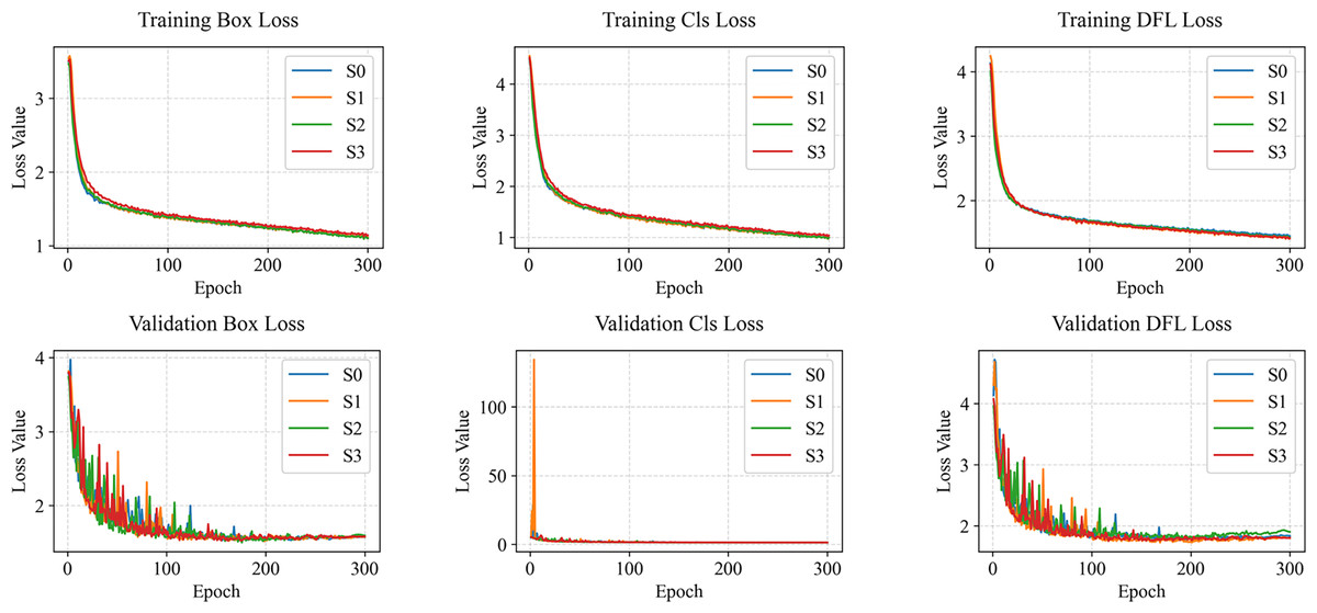
Figure 4: Loss curve comparison on NEU-DET.
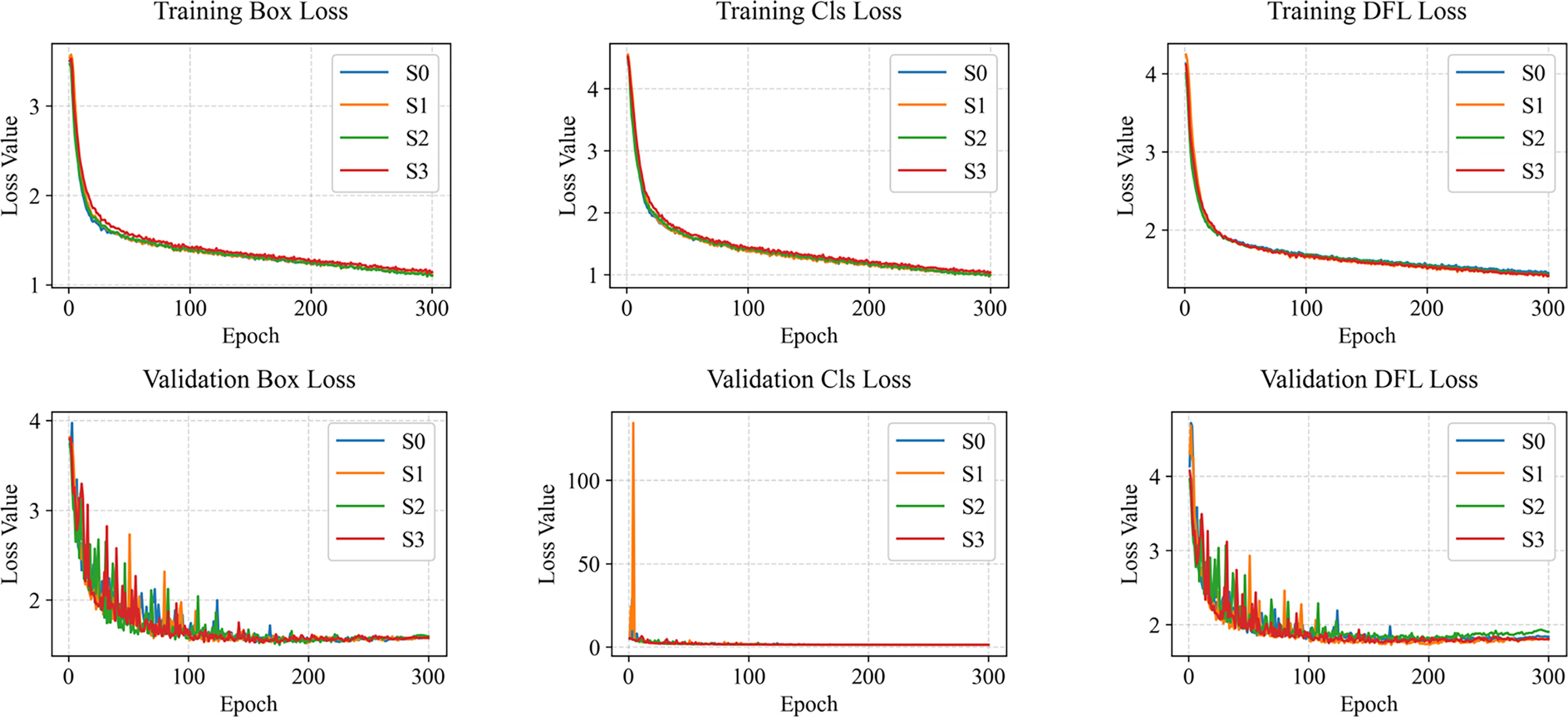
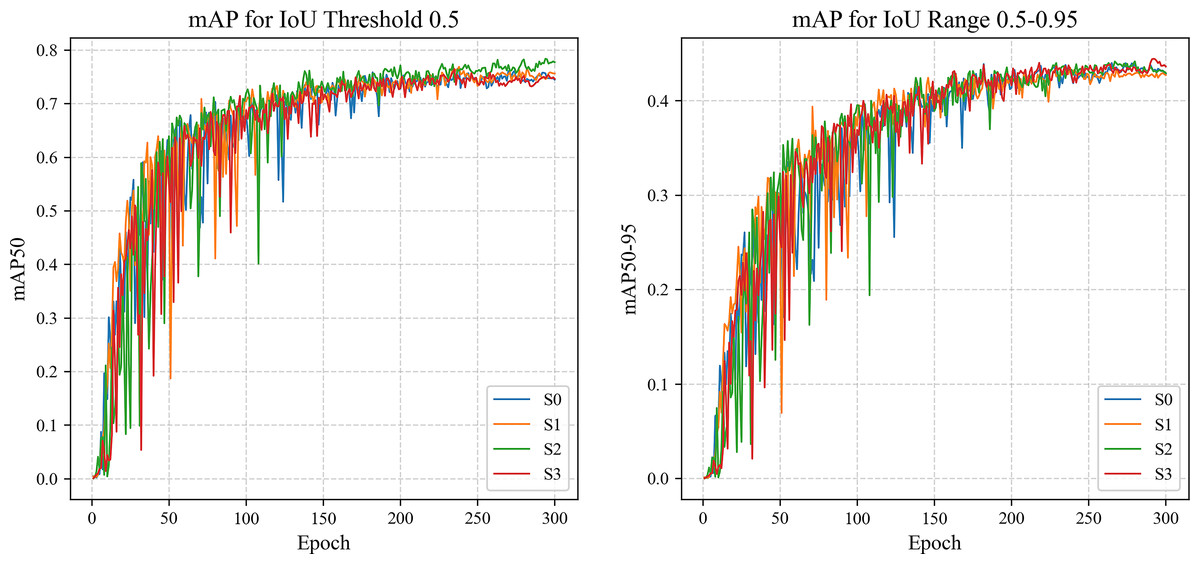
Figure 5: The mAP curve comparison on NEU-DET.
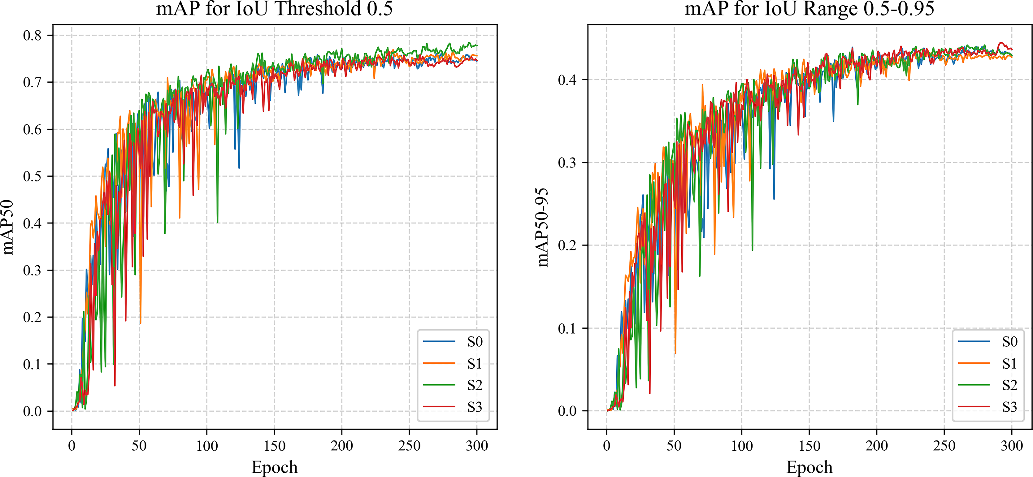
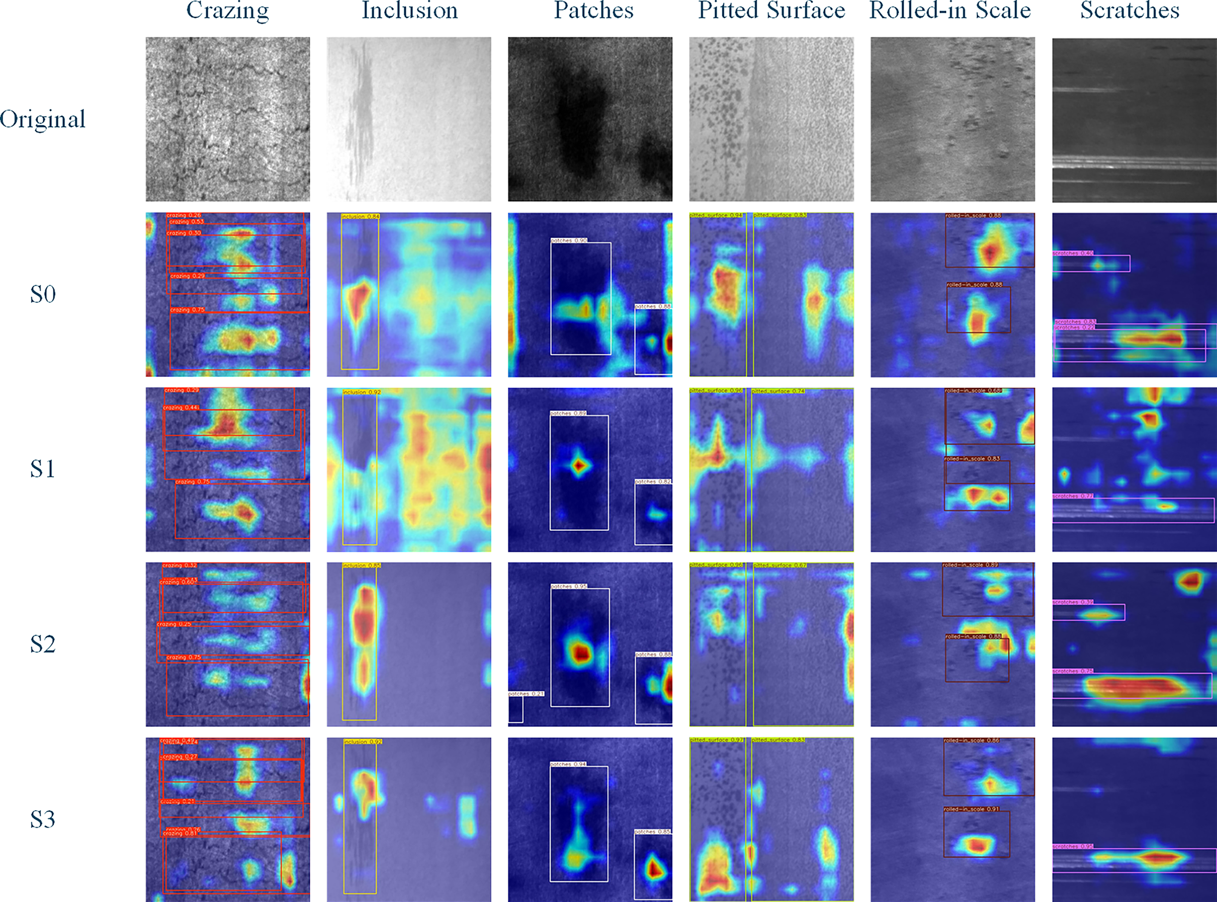
Finally, we observe the Grad-CAM heatmaps of six types of defects in the NEU-DET dataset, as shown in Fig. 6. Figure 6 indicates that LightSDD provides more comprehensive and accurate identification of key defect features.
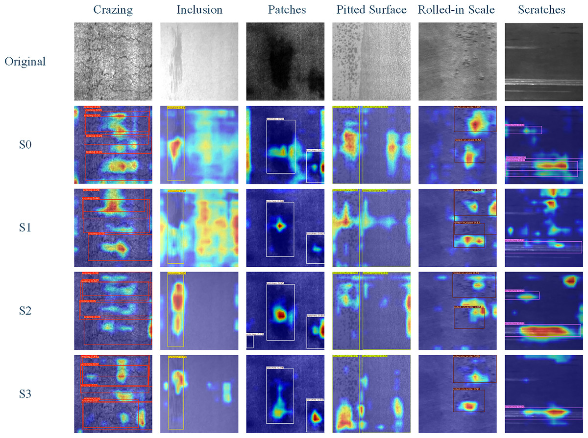
Figure 6: Grad-CAM feature response visualization of different modules on NEU-DET.
In conclusion, both C3k2_PKI and LSCD have played positive roles. The feature fusion strategy of LightSDD, which combines C3k2_PKI and LSCD, has a synergistic effect and possesses the comprehensive detection capability for targets of different scales.
Performance comparison
Seven object detection models, namely YOLOv3-tiny, YOLOv5n, YOLOv6n, YOLOv8n, YOLOv9t, YOLOv10n and YOLOv11, are selected as comparative methods. A five-fold cross-validation experiment is conducted to validate the advantages of the improved model proposed in this article. The test results on both the NEU-DET and GC10-DET datasets are presented in Table 5.
| Dataset | Algorithm | mAP50 (%) | mAP50~95 (%) | Precision (%) | Recall (%) | Parameters/M | FLOPs/G |
|---|---|---|---|---|---|---|---|
| NEU-DET | YOLOv3-tiny | 66.13 ± 1.02 | 30.74 ± 1.14 | 63.82 ± 1.98 | 64.42 ± 2.46 | 9.52 | 14.30 |
| YOLOv5n | 75.42 ± 1.29 | 41.97 ± 1.13 | 72.17 ± 1.86 | 69.99 ± 2.34 | 2.18 | 5.80 | |
| YOLOv6n | 76.83 ± 0.85 | 43.42 ± 0.85 | 70.92 ± 3.00 | 72.23 ± 1.92 | 4.16 | 11.50 | |
| YOLOv8n | 76.45 ± 1.50 | 44.20 ± 0.90 | 71.19 ± 2.68 | 72.66 ± 1.71 | 2.69 | 6.80 | |
| YOLOv9t | 77.48 ± 0.48 | 44.46 ± 1.60 | 71.27 ± 2.79 | 72.34 ± 1.60 | 1.73 | 7.40 | |
| YOLOv10n | 76.64 ± 0.74 | 42.28 ± 0.70 | 72.61 ± 2.82 | 67.71 ± 2.42 | 2.27 | 6.50 | |
| YOLOv11 | 78.00 ± 1.00 | 44.70 ± 1.10 | 74.80 ± 2.20 | 72.20 ± 2.20 | 2.58 | 6.30 | |
| LightSDD | 76.81 ± 1.25 | 44.86 ± 0.33 | 70.18 ± 0.90 | 72.70 ± 1.32 | 2.42 | 6.90 | |
| GC10-DET | YOLOv3-tiny | 58.39 ± 2.90 | 28.03 ± 1.06 | 61.73 ± 5.21 | 57.46 ± 4.26 | 9.52 | 14.30 |
| YOLOv5n | 64.27 ± 1.96 | 33.36 ± 0.98 | 65.70 ± 4.95 | 61.75 ± 2.28 | 2.18 | 5.80 | |
| YOLOv6n | 60.83 ± 6.21 | 30.49 ± 2.52 | 62.12 ± 4.52 | 59.50 ± 6.21 | 4.16 | 11.50 | |
| YOLOv8n | 64.18 ± 1.68 | 32.46 ± 0.84 | 65.25 ± 4.42 | 61.60 ± 3.23 | 2.69 | 6.80 | |
| YOLOv9t | 65.56 ± 0.39 | 33.35 ± 0.69 | 66.98 ± 2.32 | 63.13 ± 0.31 | 1.73 | 7.40 | |
| YOLOv10n | 62.93 ± 0.51 | 32.08 ± 1.14 | 68.19 ± 6.42 | 59.67 ± 2.43 | 2.27 | 6.50 | |
| YOLOv11 | 64.49 ± 2.53 | 33.19 ± 1.96 | 68.38 ± 4.05 | 62.56 ± 2.97 | 2.58 | 6.30 | |
| LightSDD | 64.92 ± 1.88 | 33.39 ± 0.81 | 66.89 ± 4.20 | 63.58 ± 2.31 | 2.42 | 6.90 |
As shown in Table 5, LightSDD achieves the highest mAP50~95 of 44.86% on the NEU-DET dataset among all compared models. With only 2.42M parameters, it reduces the parameter count by 41.80% compared to YOLOv6n (4.16M), which has the closest detection accuracy. Its computational cost (FLOPs = 6.90G) is also 40.00% lower than that of YOLOv6n (11.50G), demonstrating that the lightweight design significantly optimizes resource usage while maintaining competitive accuracy. Compared to YOLOv11, LightSDD improves mAP50~95 by 0.16% (44.70% → 44.86%), although mAP50 decreases by 1.19% (78.00% → 76.81%). This indicates that the model offers stronger robustness under stricter IoU thresholds, while the slight drop in mAP50 may result from reduced classification confidence due to lightweight compression.
Meanwhile, LightSDD demonstrates comprehensive performance advantages on the GC10-DET dataset, achieving the highest mAP50 (64.92%) and mAP50~95 (33.39%), as well as the best Recall (63.58%). Although its Precision (66.89%) is slightly lower than the top-performing YOLOv11 (68.38%), it still surpasses all other compared methods. More importantly, LightSDD shows the lowest standard deviation in both mAP50~95 and Recall, highlighting its superior stability and robustness. In terms of model efficiency, LightSDD maintains the lowest number of parameters (2.42M) and a relatively low computational cost (FLOPs = 6.90 G), further confirming its high computational efficiency.
Additionally, experiments repeatedly conducted on both the NEU-DET and GC10-DET datasets not only validate the stability and generalization capability of LightSDD across different defect distributions and complex scenarios, but also demonstrate that its performance improvement does not merely represent minor enhancements to YOLO-based baseline models. Instead, it reflects a systematic breakthrough in multi-scale feature modeling and lightweight optimization. By consistently achieving higher mAP50–95 and recall rates across diverse data characteristics, LightSDD proves its robustness and scalability, providing transferable technical references for industrial defect detection research under computational constraints. We also document the training durations from five-fold cross-validation experiments in Table 6 to facilitate the reproduction of our work by other researchers.
| Dataset | Algorithm | Fold0 | Fold1 | Fold2 | Fold3 | Fold4 | Average |
|---|---|---|---|---|---|---|---|
| NEU-DET | YOLOv3-tiny | 6,971.45 | 7,493.00 | 7,461.08 | 7,499.74 | 7,465.20 | 7,378.09 |
| YOLOv5n | 5,764.92 | 5,733.52 | 5,757.32 | 5,754.16 | 5,725.61 | 5,747.11 | |
| YOLOv6n | 5,454.67 | 5,456.54 | 5,417.8 | 5,399.56 | 5,473.55 | 5,440.42 | |
| YOLOv8n | 5,888.91 | 5,920.26 | 5,882.08 | 5,841.42 | 5,885.97 | 5,883.73 | |
| YOLOv9t | 8,229.87 | 9,968.86 | 7,625.21 | 8,137.96 | 7,978.56 | 8,388.09 | |
| YOLOv10n | 6,841.56 | 5,862.23 | 6,522.06 | 6,275.72 | 6,173.47 | 6,335.01 | |
| YOLOv11 (S0) | 6,438.31 | 6,425.62 | 6,456.93 | 6,422.37 | 6,463.28 | 6,441.30 | |
| S1 | 12,344.00 | 12,362.40 | 12,415.00 | 12,352.50 | 12,335.60 | 12,361.90 | |
| S2 | 5,932.84 | 6,004.59 | 5,955.66 | 6,059.29 | 6,009.08 | 5,992.29 | |
| LightSDD | 12,179.40 | 12,127.40 | 11,903.90 | 11,968.70 | 12,014.50 | 12,038.78 | |
| GC10-DET | YOLOv3-tiny | 6,540.65 | 7,951.13 | 7,868.44 | 7,439.26 | 7,721.78 | 7,504.25 |
| YOLOv5n | 7,159.08 | 7,037.18 | 7,250.41 | 7,196.69 | 7,294.73 | 7,187.62 | |
| YOLOv6n | 6,837.28 | 7,351.63 | 7,629.50 | 6,920.58 | 10,165.80 | 7,780.96 | |
| YOLOv8n | 4,731.14 | 7,460.40 | 7,389.63 | 7,403.11 | 7,461.65 | 6,889.19 | |
| YOLOv9t | 11,378.60 | 11,527.70 | 11,210.30 | 11,172.90 | 11,039.10 | 11,265.72 | |
| YOLOv10n | 10,264.40 | 9,789.40 | 10,232.50 | 10,200.30 | 10,548.80 | 10,207.08 | |
| YOLOv11 | 6,485.93 | 7,673.41 | 7,745.76 | 7,713.25 | 7,712.11 | 7,466.09 | |
| LightSDD | 14,125.50 | 13,598.80 | 14,210.50 | 13,022.10 | 14,082.40 | 13,807.86 |
In summary, LightSDD achieves an effective balance between accuracy and efficiency in steel surface defect detection tasks, offering leading comprehensive accuracy, high stability, and notable lightweight characteristics.
Performance testing on edge devices
To evaluate the performance of the proposed LightSDD on edge devices, this section deploys LightSDD to the mobile terminal Samsung Galaxy S23 Ultra using the NCNN framework. The basic configuration of Samsung Galaxy S23 Ultra is as follows: Snapdragon 8 Gen 2 processor, 8GB RAM, 256GB ROM, and Android 16.0 operating system. First, the model weights trained under the PyTorch framework are converted into a format compatible with the NCNN framework. Subsequently, inference code is developed in C++ based on the NCNN inference framework. Finally, the APK file is built and generated using Android Studio. The development tools used during the deployment process are listed in Table 7.
| Development tool | Description |
|---|---|
| NCNN | A deep learning model deployment framework optimized for mobile and embedded devices |
| Cmake | A cross-platform compilation tool used to install and compile third-party libraries |
| JNI | Java Native Interface for integrating C++ code into Java programs |
| Vulkan | A deep learning computing acceleration library suitable for the NCNN framework |
After installing the LightSDD package compiled by Android Studio on the Samsung Galaxy S23 Ultra, 30 image samples were randomly selected from the NEU-DET test set for verification, with five samples per category. The test results are shown in Table 8, and the detection effects are illustrated in Fig. 7. As shown in Table 8, LightSDD exhibits excellent inference efficiency across various input resolutions, achieving near real-time detection performance that meets the stringent speed requirements of industrial production lines. Furthermore, the model’s memory usage during operation remains consistently below 5MB, indicating that its lightweight design effectively controls memory overhead, aligning well with the resource-constrained nature of edge devices. From the detection examples shown in Fig. 7, it can be shown that the model accurately identifies and locates all six types of defects in the NEU-DET dataset. These results demonstrate superior detection effectiveness, indicating that the model possesses strong robustness and practical applicability.
| Input resolution | FPS | Avg inference time/ms | Memory usage/MB |
|---|---|---|---|
| 640 640 | 30~35 | 16.02 | 4.96 |
| 480 | 34~39 | 15.20 | 4.59 |
| 320 | 35~43 | 13.05 | 4.24 |
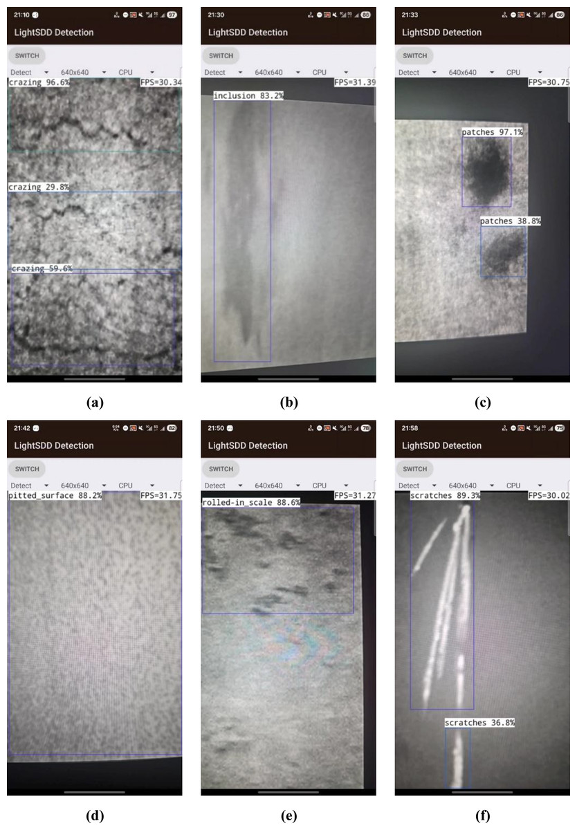
Figure 7: Detection examples on edge devices using the NEU-DET dataset.
(A) Crazing category, (B) Inclusion category, (C) Patches category, (D) Pitted Surface category, (E) Rolled-in Scale category, (F) Scratches category.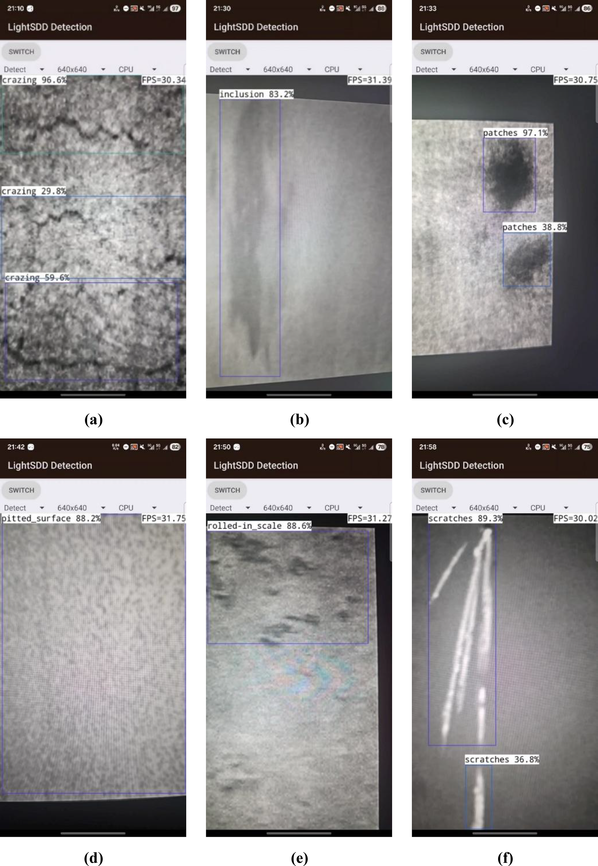
Discussion
The core innovation of LightSDD lies in its synergistic optimization of multi-scale dynamic perception and lightweight cross-stage fusion. The proposed C3k2_PKI module enhances feature representation capability for tiny and multi-scale defects through multi-scale dynamic convolutional kernels and attention weighting, increasing the recall rate to 72.70%. The LSCD detection head effectively maintains and improves key positioning accuracy while reducing parameters via channel compression, cross-resolution feature alignment and concatenation, and group convolution. Furthermore, a dynamic parameter control mechanism ensures the model’s efficient inference potential on edge devices. This co-design enables LightSDD to achieve an optimal balance among detection accuracy, recall rate, and model lightweighting.
Although LightSDD demonstrates certain advantages across both datasets, it still exhibits some limitations. We analyze the failure cases illustrated in Fig. 8, where Figs. 8A and 8B are the detection images of crack categories, Figs. 8C and 8D are the detection images of plaque categories, and Figs. 8E and 8F are the detection images of scratch categories. Observing Fig. 8, it reveals that channel compression in LSCD weakens the discriminability of fine-grained textures, leading to the misclassification of crack fracture patterns as discrete patches (Figs. 8A, 8B). Both patches and inclusions initially exhibit clustered point-wise distributions, but the group convolution operation blurs the local features of small-sized targets. Combined with interference from background oxide scale textures, this results in category confusion for the model (Figs. 8C and 8D). In the detection of scratch-type defects, the fluctuation in accuracy essentially stems from the interaction between the lightweight architecture and the multi-scale nature of defect characteristics. Scratches are typically slender and exhibit low contrast, making them susceptible to interference from the background. Moreover, channel compression partially reduces the model’s sensitivity to subtle textures. Meanwhile, the architectural design intentionally prioritizes a high-recall strategy. The use of large convolutional kernels (C3k2_PKI) benefits the detection of long-range continuous targets, such as scratches, but at the cost of reduced local boundary accuracy. This results in an 8.60% decrease in accuracy for defects sensitive to positioning, such as pitting, while scratches, which rely more on continuity features, experience only a 2.90% decrease (Figs. 8E and 8F). The increase in FLOPs of LightSDD is primarily attributed to the multi-scale dynamic convolution design in the C3k2_PKI (Yang et al., 2020). This design enhances the model’s perception of subtle defects through the parallel deployment of multi-scale convolutional kernels (Yang & Liu, 2022), especially under complex backgrounds, boosting the recall rate to 72.70%. Although the multi-scale dynamic convolution increases computational cost, the model maintains its feasibility on edge devices through parameter compression and dynamic inference optimization.
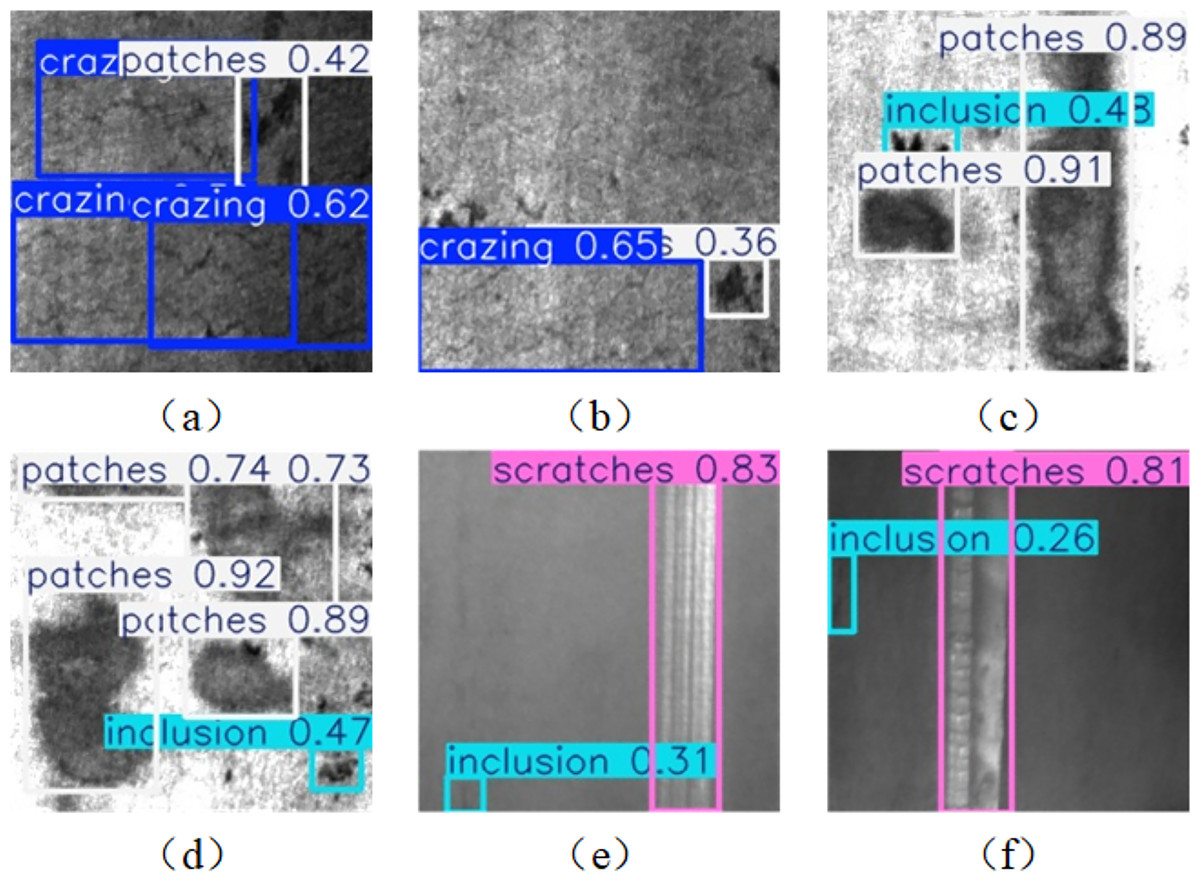
Figure 8: Failure case examples.
(A) and (B) show detection images of crack category, (C) and (D) display detection images of patch category, (E) and (F) exhibit detection images of scratch category.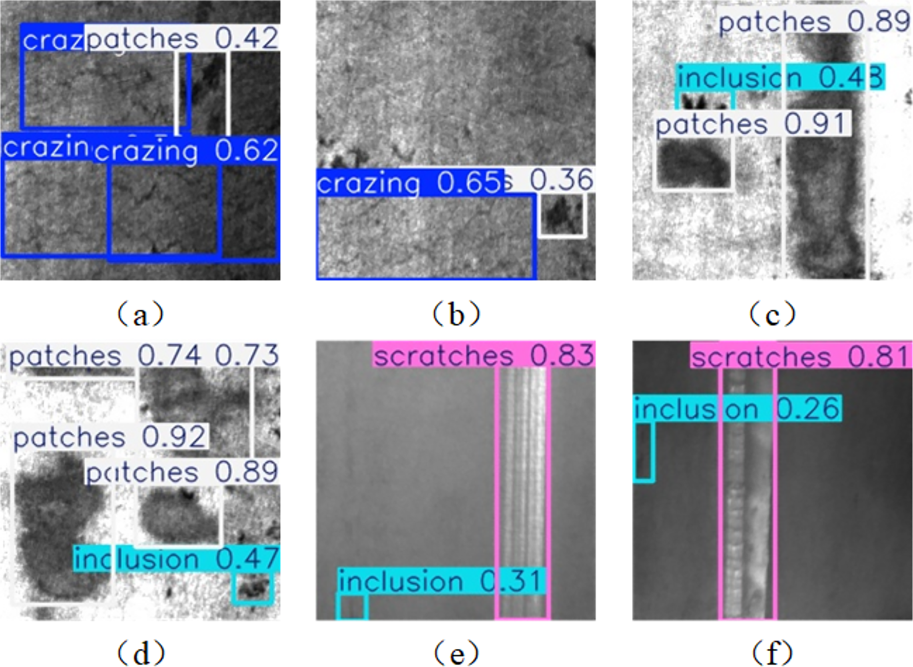
Future research can deepen exploration from two dimensions: First, to address the decline in texture discrimination caused by lightweight compression, a module integrating asymmetric convolution and multi-scale gradient feature extraction can be designed. This would enhance the local contrast response to shallow defects and improve detection sensitivity for low-contrast defects such as pitting and faint scratches. Second, introducing auxiliary sensing data such as thermal imaging or laser scanning can be considered to establish a multimodal fusion-based false detection correction mechanism. This would help resolve morphological confusion between fractured scratches and inclusions. Furthermore, counterfactual explanations and prototype-based explainable methods (Xu & Yang, 2025) can be designed, which would help enhance the transparency of the model and promote human-machine collaboration in industrial quality inspection.
Conclusion
LightSDD proposed in this article effectively addresses the challenge of balancing multi-scale object detection accuracy with real-time performance on edge devices in industrial scenarios through a dynamic convolution optimization module (C3k2_PKI) and a lightweight cross-stage detection head (LSCD). Experimental results on the NEU-DET dataset show that LightSDD achieves a mAP50~95 of 44.86%, outperforming the baseline YOLOv11 by 0.16% and reducing parameters by 6.20%. On the GC10-DET dataset, it achieves a mAP50~95 of 33.39%, outperforming the baseline YOLOv11 by 0.20%, with a parameter reduction of 6.20%. The C3k2_PKI module adaptively enhances the feature representation capability for small objects by multi-scale dynamic convolutional kernels (ranging from 3 × 3 to 11 × 11). Meanwhile, through channel compression (256→128) and cross-stage feature fusion, the LSCD detection head reduces computational costs while maintaining positioning accuracy for complex defects such as pitted surfaces.