
Contrast-enhanced MRI segmentation and classification with optimized vector machine classifier
- Published
- Accepted
- Received
- Academic Editor
- Consolato Sergi
- Subject Areas
- Algorithms and Analysis of Algorithms, Artificial Intelligence, Computer Vision, Data Mining and Machine Learning, Neural Networks
- Keywords
- Diffusion filtering, Fast-marching method, Support vector machine, Brain tumor, Contrast-enhanced magnetic resonance imaging, Optimized computational efficiency, Brain tumor detection, CE-MRI, FMM, Segmentation
- Copyright
- © 2026 Asiri et al.
- Licence
- This is an open access article distributed under the terms of the Creative Commons Attribution License, which permits unrestricted use, distribution, reproduction and adaptation in any medium and for any purpose provided that it is properly attributed. For attribution, the original author(s), title, publication source (PeerJ Computer Science) and either DOI or URL of the article must be cited.
- Cite this article
- 2026. Contrast-enhanced MRI segmentation and classification with optimized vector machine classifier. PeerJ Computer Science 12:e3482 https://doi.org/10.7717/peerj-cs.3482
Abstract
Brain tumors are a significant cause of mortality worldwide, highlighting the need for accurate and efficient diagnostic tools. Magnetic Resonance Imaging (MRI) and Computed Tomography (CT) provide valuable imaging data; however, manual interpretation remains labor-intensive and prone to variability. This study introduces an automated framework for brain tumor detection that integrates image enhancement, segmentation, and classification. Preprocessing is performed using Contrast-Limited Adaptive Histogram Equalization (CLAHE) and diffusion filtering to improve image clarity. Tumor regions are segmented through the Fast Marching Method (FMM), and classification is carried out using an optimized Support Vector Machine (SVM). Evaluation on a Contrast-Enhanced Magnetic Resonance Imaging (CE-MRI) dataset covering gliomas, meningiomas, and pituitary tumors demonstrates strong results, with sensitivity of 0.98, specificity of 0.99, overall accuracy of 98.6%, and a Dice Similarity Coefficient (DSC) of 0.963. The proposed method achieves high performance while reducing processing time to 0.43 s per image, surpassing several existing techniques. These findings indicate that the framework offers a practical and efficient solution for clinical brain tumor diagnosis, with potential for further improvements through integration of multiple classifiers to enhance robustness.
Introduction
The rapid advancement of digital medical technologies has significantly transformed healthcare delivery, particularly within the domain of e-health, where automated image analysis now plays a crucial role in early disease detection and diagnosis. Among various imaging modalities, medical imaging has become indispensable for identifying abnormalities in vital organs, with the brain representing one of the most challenging yet essential areas of focus due to its structural complexity and its central role in regulating bodily functions (Alqhtani et al., 2024b; Budati & Katta, 2022). Within neurological disorders, brain tumors pose a particularly serious concern. These tumors are characterized by uncontrolled cellular proliferation that interferes with normal brain activity, severely compromising patient health and quality of life (Alqhtani et al., 2024a; Yao, Zhang & Xu, 2016). Detecting tumors at an early stage with high precision is therefore critical for guiding effective treatment planning and improving patient outcomes, as delays in diagnosis are frequently associated with irreversible neurological impairments (Indira et al., 2020) or even mortality (Asiri et al., 2024; Armstrong et al., 2004).
Magnetic Resonance Imaging (MRI) has emerged as the preferred modality for brain tumor assessment because it is non-invasive, provides superior soft-tissue contrast, and offers high spatial resolution, all of which are essential for visualizing subtle abnormalities in brain structures (Kim et al., 2015). By comparison, Computed Tomography (CT) remains effective for examining bone-related pathology but is susceptible to noise artifacts, limiting its capacity to resolve fine anatomical details with precision (Lundervold & Lundervold, 2019; Jiang, Hou & Deng, 2018; Hssayeni, 2020). MRI, in contrast, provides multi-dimensional visualization of brain tissue and ensures greater reliability in identifying intracranial lesions. Figure 1 illustrates a side-by-side comparison of CT and MRI scans (Babu, Nagajaneyulu & Prasad, 2021), highlighting the clear advantages of MRI, particularly in terms of lesion visibility, noise suppression, and enhanced contrast that facilitate accurate tumor detection (Lather & Singh, 2020).
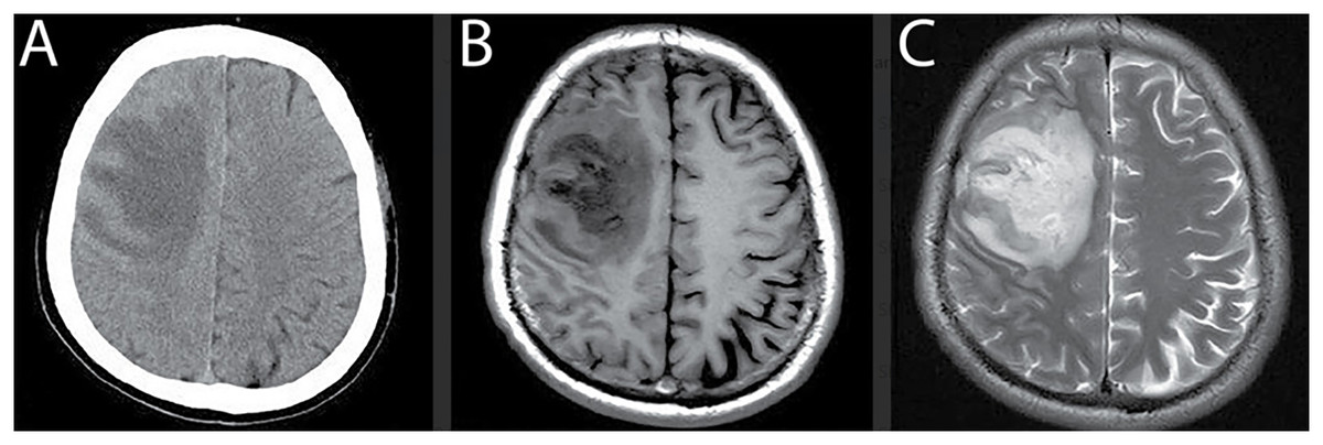
Figure 1: Comparison of MRI and CT brain scans for tumor detection.
(A) CT scan shows reduced density in the right frontal lobe with lower contrast and noise artifacts, limiting the ability to differentiate soft tissue structures. (B) and (C) T1- and T2-weighted MRI scans provide improved visualization of the lesion with higher contrast, reduced noise, and better differentiation between gray and white matter, enhancing the accuracy of tumor diagnosis.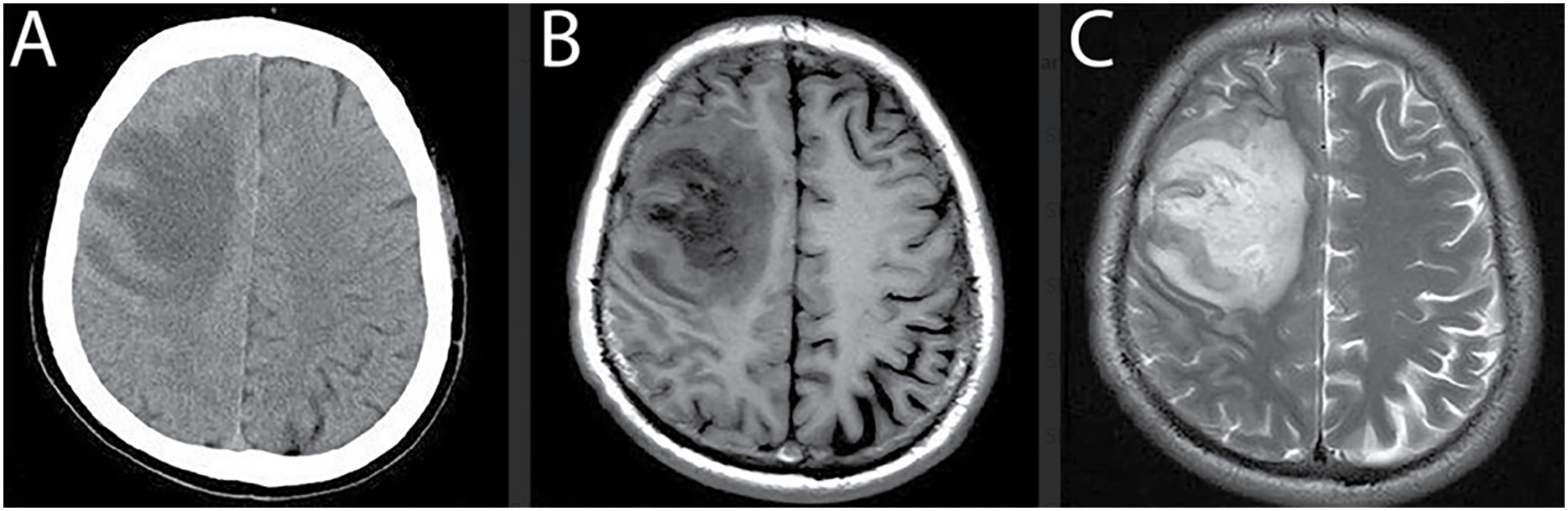
Note: All MRI images presented in this manuscript are sourced from the publicly available Brain Tumor CE-MRI dataset at Figshare https://figshare.com/articles/dataset/brain_tumor_dataset/1512427.
Over recent decades, computer-assisted diagnostic methods have been increasingly developed to assist radiologists in the detection and delineation of brain tumors in MRI scans. Traditional machine learning techniques, such as K-Nearest Neighbor (KNN) (Qasem, Nazar & Attia Qamar, 2019) and Self-Organizing Maps (SOM) (Logeswari & Karnan, 2010), were among the early approaches employed for segmentation tasks. However, these methods often suffer from key limitations, including intensity inhomogeneity, poor image contrast, and substantial computational demands. More recent advances in deep learning, particularly Convolutional Neural Networks (CNNs) (Khan et al., 2021; Deng et al., 2019) and hybrid CNN–Long Short-Term Memory (CNN-LSTM) architectures (Wang et al., 2023), have demonstrated strong performance in brain tumor classification. Despite their high accuracy, these models demand extensive labeled datasets, powerful computational resources, and long training times, making them less feasible for real-time clinical applications. Additionally, persistent challenges such as noise interference, variation in tumor intensity, and complex feature extraction remain unresolved (Badran, Mahmoud & Hamdy, 2010; Rajesh Babu et al., 2019; Kundana Gowri Rajesh Babu et al., 2020). These gaps underscore the need for hybrid frameworks that balance segmentation precision, classification robustness, and computational efficiency.
To address the limitations of existing methods, this study introduces an automated framework that integrates the Fast Marching Method (FMM) for segmentation with the Support Vector Machine (SVM) for classification. The proposed FMM SVM pipeline is designed to detect, segment, and classify brain tumors in MRI scans with high precision and reduced computational burden. FMM provides smooth and reliable boundary propagation without the need for manual initialization or iterative contour refinement, which makes it more stable than thresholding based approaches that struggle with intensity inconsistencies. The classification stage is carried out using SVM, which leverages a refined set of handcrafted features to differentiate tumor from non tumor regions with strong accuracy and efficiency.
Although hybrid models such as FCM SVM and CNN SVM combinations have been reported (Zhao et al., 2018), they continue to face several challenges. FCM based methods are often sensitive to intensity inhomogeneity and require repeated updates that can destabilize segmentation, especially in regions with weak boundary definition. CNN SVM models, while effective, depend heavily on large annotated datasets and substantial computational resources, which limits their practical use in environments where such resources are unavailable. The framework proposed in this study directly addresses these difficulties by employing FMM for stable and computationally efficient boundary extraction and SVM for accurate classification without reliance on deep feature learning or large scale training. This design provides an interpretable, lightweight, and practical alternative for real world clinical applications.
The contributions of this study include the development of a fully automated five stage pipeline that combines preprocessing, segmentation, classification, and post processing for complete tumor detection. The approach offers precise tumor boundary extraction using FMM and reliable region classification using SVM trained on optimized handcrafted features. The framework is evaluated on a CE MRI dataset comprising gliomas, meningiomas, and pituitary tumors, demonstrating strong performance across these categories. Notably, the method achieves a Dice Similarity Coefficient of 0.963, high accuracy and specificity, and an average processing time of 0.43 s per image, which highlights its suitability for real time clinical use.
The FMM SVM strategy developed in this work provides a resource conscious alternative to deep learning based pipelines by combining classical image processing with statistical learning in a unified manner. The segmentation stage adapts naturally to intensity gradients and yields coherent tumor outlines, while the classification stage efficiently distinguishes abnormal from healthy tissue with minimal computational overhead. This combination results in a robust and scalable solution for automated tumor detection. By integrating FMM based segmentation with SVM based classification, the proposed system achieves an overall accuracy of 98.6 percent, supported by a reproducible five stage workflow that begins with noise reduction and contrast enhancement to ensure consistent image quality throughout the process.
The remainder of this manuscript is structured as follows. ‘Related Literature Review’ provides a detailed review of existing literature on brain tumor segmentation and classification, covering both traditional machine learning and deep learning techniques. ‘Materials and Proposed Method’ introduces the proposed FMM-SVM framework, with emphasis on preprocessing, segmentation, classification, and post-processing strategies. ‘Results and Discussion’ describes the experimental design, including dataset description, parameter optimization, and implementation details. ‘Discussion: Model Evaluation, Challenges, and Directions for Optimization’ presents the results and a comparative discussion against state-of-the-art approaches, highlighting the performance advantages of the proposed method. Finally, ‘Conclusion and Translational Implications for Clinical Integration’ and summarize the study’s key findings, outline its practical implications, and suggest potential directions for future work, including the integration of multi-modal imaging and the incorporation of deep learning enhancements for further robustness in tumor classification.
Related literature review
Brain tumor segmentation and classification in MRI scans remain challenging tasks due to intensity inhomogeneity, structural variability, and limited annotated datasets. Numerous methods have been proposed to address these challenges (Soomro et al., 2023), yet many still face issues related to generalizability, computational cost, or sensitivity to noise. Earlier approaches focused heavily on optimization-driven and clustering-based techniques. For instance, a computerized system employing Harmony Search Optimization to train a multi class Support Vector Neural Network (multi-SVNN) was introduced in Raju, Suresh & Rao (2018). This method also incorporated Bayesian fuzzy clustering to automatically identify tumor regions, although its evaluation was restricted to the BraTS dataset, limiting its broader applicability. Similar investigations involving Harmony Search Optimization combined with clustering strategies demonstrated improvements over traditional methods (Logeswari & Karnan, 2010; Chaithanyadas & Gnana King, 2022), but their dependence on small sample sizes constrained their generalization to diverse MRI datasets. These optimization-based studies established foundational concepts but highlighted the need for more robust segmentation mechanisms that operate reliably across varying imaging conditions.
Subsequent research introduced more complex hybrid systems that combined clustering, neural networks, and metaheuristic optimization. Yin, Wang & Abza (2020) proposed a three-stage method involving background adjustment, region delineation, and classification using a multi layered neural network enhanced by cetacean-inspired optimization techniques. Despite its methodological novelty, the system did not significantly improve classification accuracy. A related direction was explored in Alagarsamy et al. (2019), where the Bat Algorithm and Interval Type 2 Fuzzy C Means (BAT IT2FCM) were used to improve segmentation. While this approach enhanced cluster-level accuracy, it required computationally intensive iterations and was sensitive to threshold settings, reducing its practicality for clinical workflows. These studies demonstrated the potential of optimization-assisted frameworks but also revealed their limitations in terms of execution time and adaptability.
To overcome the constraints of clustering-based pipelines, researchers shifted toward methods integrating feature selection, neural learning, and probabilistic reasoning. The WCFS IBMDNL framework introduced in Kumar et al. (2019) applied weighted correlation-based feature selection with an Iterative Bayesian Multivariate Deep Neural Network. Although the system improved initial-stage tumor classification, it struggled to accurately pinpoint tumor pixels, reducing its diagnostic reliability. Fusion-based models also gained traction, such as the neutrosophic CNN framework developed by Ozyurt et al. (2019), which combined multiple classifiers including CNN, SVM, and KNN. Although the fusion improved detection rates, architectural inconsistencies in the CNN component affected classification stability. These developments underscored the challenge of designing hybrid systems that balance accuracy, consistency, and computational efficiency.
Other researchers explored transform-based and adaptive fuzzy inference approaches to improve segmentation. Selvapandian & Manivannan (2018) employed the non-subsampled contourlet transform (NSCT) followed by ANFIS to classify brain tumors, producing satisfactory segmentation but limited by dependence on morphological operators. Sharif et al. (2020b) developed a skull-stripping and tumor extraction pipeline using BSE, PSO, and ANN classification. Although effective for certain cases, the method struggled with consistent substructure optimization. These studies indicate that hand-engineered pipelines, although interpretable, often face challenges in balancing robustness and scalability.
Hybrid clustering and neural network combinations have also been widely examined. Sharma, Purohit & Mukherjee (2018) used a combination of k-means clustering and ANN with GLCM-based features, achieving improved segmentation but failing to consistently detect tumors with very small pixel footprints. Varuna Shree & Kumar (2018) integrated probabilistic neural networks with discrete wavelet transformations to improve classification accuracy. Although the system reduced segmentation complexity, further validation on larger datasets was recommended. These hybrid frameworks provided useful insights but revealed limitations that arise when traditional feature engineering is combined with shallow learning models.
More recent efforts have shifted toward deep learning and multi-phase hybrid models that integrate feature extraction, segmentation, and classification. A two-phase system described in Abd-Ellah et al. (2018) used CNN-based feature extraction followed by ECOC-SVM classification, achieving high accuracy on BraTS and RIDER datasets, with AlexNet outperforming VGG variants. Rani & Kamboj (2019) explored Otsu thresholding with SVM classification, but encountered performance limitations. Torres-Molina et al. (2019) demonstrated that kernel-based SVM using a Gaussian RBF kernel improved accuracy and specificity. Deep learning models such as CNNs (Khan et al., 2021) and hybrid CNN-LSTM networks (Wang et al., 2023) have achieved high segmentation accuracy, but their reliance on large annotated datasets, long training times, and high hardware requirements make them less accessible outside well-resourced environments. Traditional machine learning models like KNN (Qasem, Nazar & Attia Qamar, 2019) and SOM (Logeswari & Karnan, 2010) lack adaptability to the complex intensity patterns characteristic of medical imaging.
More importantly, post-2022 studies emphasize the use of hybrid deep learning and metaheuristic algorithms, yet they still face challenges related to generalization, computational overhead, and reliance on deep feature learning. This gap highlights the need for efficient alternatives that can perform reliably without extensive training data or high-end hardware. The FMM SVM pipeline proposed in this study directly addresses these challenges by combining fast, stable segmentation with computationally efficient classification. Unlike thresholding-based segmentation approaches, FMM dynamically adapts to intensity changes and identifies tumor boundaries with precision. Furthermore, the use of optimized SVM-based feature extraction offers improved accuracy compared with clustering approaches such as FCM (Alam et al., 2019) and conventional SVM models (Latif et al., 2022). The proposed method serves as a lightweight yet robust alternative to deep learning systems, making it particularly valuable in settings with limited computational resources.
Despite considerable progress in the field, persistent challenges such as noise reduction, contrast enhancement, and the balance between computational efficiency and diagnostic accuracy remain. The limitations of existing techniques underline the need for improved methodologies that can achieve high performance while maintaining practical feasibility. Motivated by this, the present study introduces a unified FMM SVM framework that demonstrates enhanced performance across key metrics and offers a reliable solution for automated tumor detection. The next section describes the methodology in detail and outlines the main components of the proposed pipeline.
Materials and proposed method
Material: contrast-enhanced MRI database
This study makes use of a publicly available dataset (Cheng et al., 2015) (Brain Tumor CE-MRI Dataset; https://figshare.com/articles/dataset/brain_tumor_dataset/1512427) consisting of contrast-enhanced magnetic resonance imaging (CE-MRI) scans, specifically aimed at the analysis and classification of brain tumors. CE-MRI is a powerful imaging technique that uses injectable contrast agents to improve the clarity and differentiation of soft tissue structures. This contrast enhancement plays a vital role in highlighting tumor regions, making it highly beneficial for accurate diagnosis and boundary identification in brain imaging tasks.
The dataset employed was curated through clinical collaboration at Nanfang Hospital in Guangzhou and the General Hospital affiliated with Tianjin Medical University in China, collected over the span of 5 years (2005–2010). It comprises a total of 3,064 post-contrast T1-weighted brain MR images, drawn from 233 patients. These cases encompass three major tumor types: gliomas (1,426 scans), meningiomas (708 scans), and pituitary adenomas (930 scans). The imaging data was acquired at a resolution of pixels, with an in-plane spatial resolution of and a slice gap of 1 mm.
Each scan underwent manual annotation by a panel of three expert radiologists. Their segmentation efforts were integrated into a consensus ground truth, ensuring high-quality, expert-validated tumor region identification. The dataset was randomly divided into training (70%), validation (15%), and testing (15%) sets, ensuring that images from the same patient were not distributed across different subsets to avoid data leakage.
Beyond its clinical richness, this dataset serves as a valuable resource for the development of deep learning algorithms targeting medical image segmentation, classification, and tumor detection. Its structure and annotations make it especially suitable for evaluating methods under real-world imaging conditions. In comparison to other public repositories such as ADNI and TCIA, this CE-MRI collection provides focused, well-curated data specifically tailored for brain tumor analysis. Representative samples from the dataset are visualized in Fig. 2, depicting typical appearances of the three tumor types captured in contrast-enhanced scans.
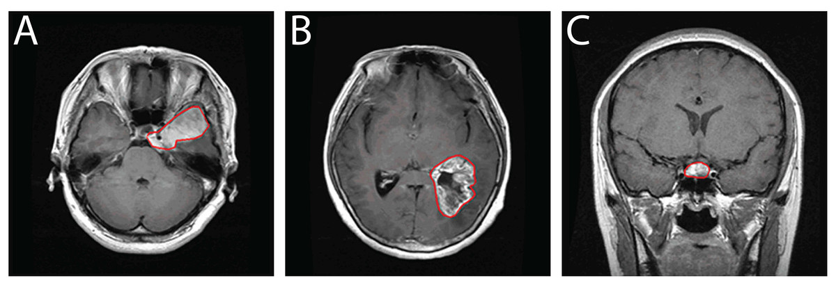
Figure 2: Sample CE-MRI brain scans: (A) Meningioma, (B) Glioma, (C) Pituitary tumor.
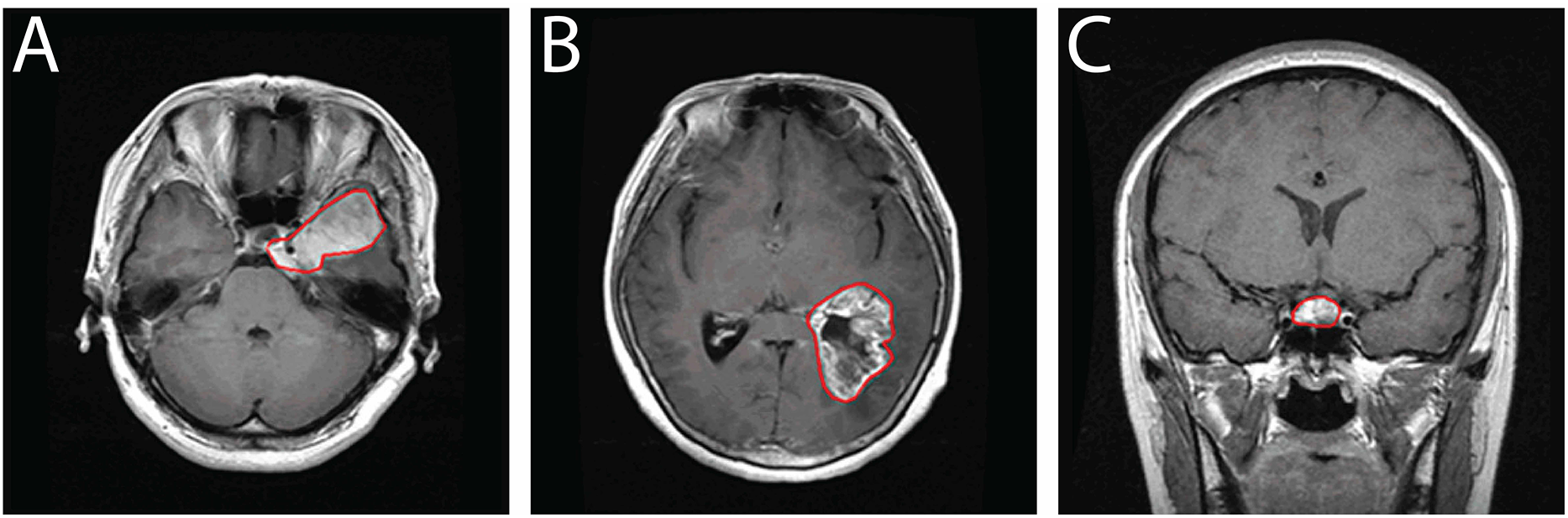
Proposed method
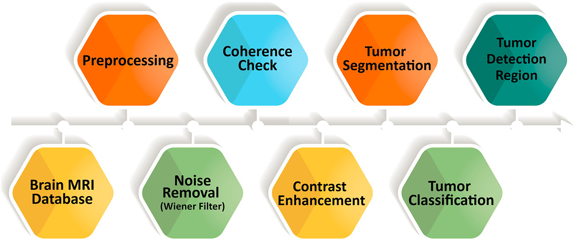
MRI provides detailed structural information that is essential for reliable brain tumor detection; however, manual interpretation can be slow and prone to inconsistency. To overcome these limitations, we introduce a fully automated five-stage framework that integrates FMM for segmentation and SVM for classification. The complete workflow is shown in Fig. 3, outlining the process from initial image enhancement to final tumor categorization.
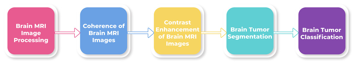
Figure 3: Overview of the sequential steps in the proposed brain MRI analysis pipeline.
The process begins with preprocessing to suppress noise and improve image clarity, followed by coherence enhancement to ensure uniform structural representation. Contrast enhancement highlights tumor-related features, after which tumor regions are segmented and classified into specific categories.
The FMM–SVM framework is designed to provide accurate segmentation, reliable classification, and efficient computation. FMM traces tumor boundaries through a smooth, adaptive front-propagation strategy without requiring manual initialization. SVM then classifies tumor and non-tumor regions using feature vectors derived from the segmented areas. Unlike deep learning models that depend on extensive labeled datasets and significant computational resources, this hybrid approach offers competitive performance with lower computational demand.
The methodology proceeds through five sequential stages. First, MRI scans undergo preprocessing for intensity correction and noise removal. Second, oriented diffusion filtering enhances coherence across tissues while preserving tumor structures. These steps improve image quality and support stable segmentation. In the third stage, the Fast Marching Method is applied to generate binary segmentation masks by treating the boundary-detection task as an evolving front. The fourth stage performs SVM-based classification using extracted tumor features, enabling clear differentiation between normal and abnormal tissue. Finally, post-processing refines the segmented regions and further stabilizes classification performance.
Through the combination of rapid boundary detection and robust classification, the proposed FMM–SVM pipeline delivers precise tumor localization with minimal manual intervention and reduced processing time. Its accuracy, efficiency, and scalability make it a suitable candidate for real-time clinical environments, outperforming conventional segmentation techniques and many computationally intensive learning-based alternatives.
Brain MRI image processing using Wiener filtering
Preprocessing is a vital stage in medical image analysis, serving to improve the quality of MRI scans before segmentation and classification. In this study, an adaptive Wiener filter is utilized to suppress noise, such as acquisition artifacts, scanner distortions, and thermal fluctuations, while maintaining the integrity of important anatomical structures. MRI slices from axial, sagittal, and coronal orientations are processed using a neighborhood window to capture localized intensity variations. The Wiener filter adjusts its response based on regional statistics, effectively smoothing noise in uniform areas while preserving sharper transitions at tissue interfaces. This balance is essential for maintaining boundary information, which is crucial for accurate tumor delineation in subsequent stages of the pipeline.
Figure 4 provides a visual comparison illustrating the effect of Wiener filtering. The top row shows the original noisy images across the three orientations, while the bottom row displays the corresponding denoised outputs. The filtered images exhibit enhanced uniformity, clearer structural definition, and substantial noise reduction, all of which contribute to improved reliability in later processing steps. To ensure methodological transparency, the mathematical formulation of the Wiener filter and its implementation details are presented in “Wiener Filtering Equations”. These refined images form a stable foundation for the next phase of the workflow, which involves contrast enhancement.
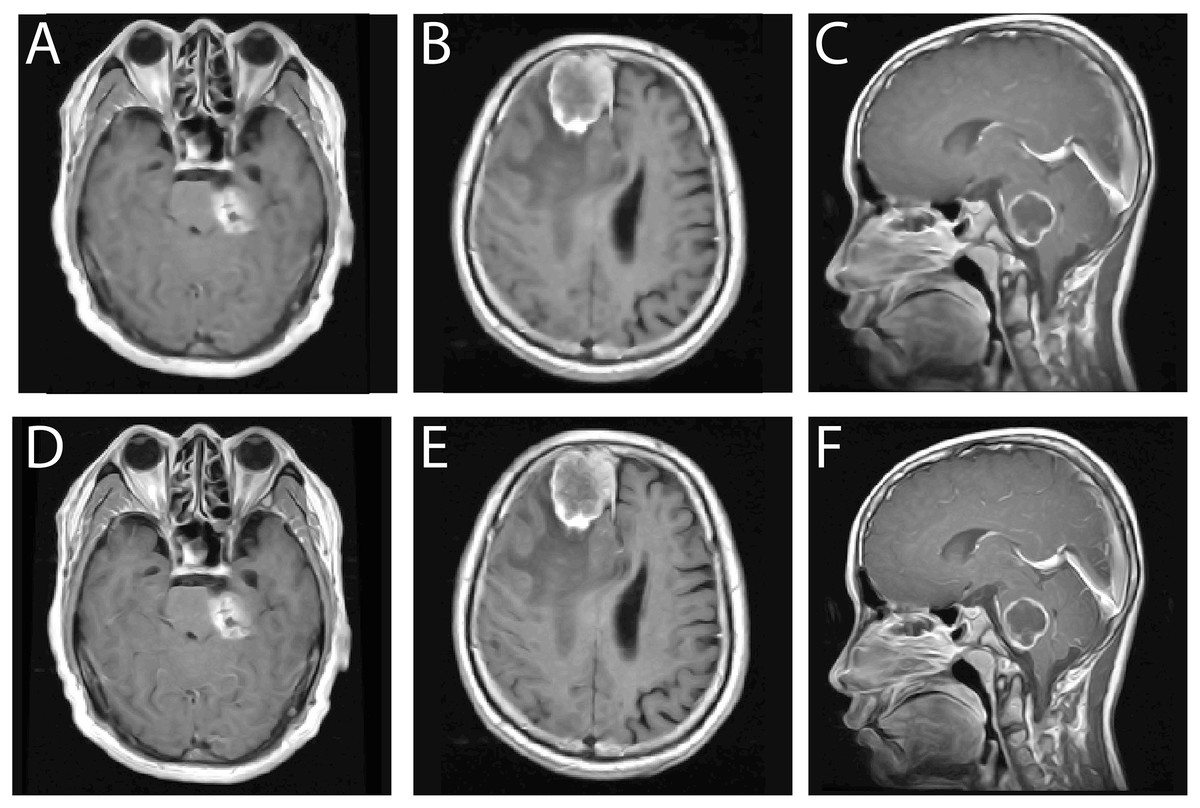
Figure 4: Comparison of MRI brain images before and after Wiener filtering across axial, sagittal, and coronal views.
Top row (A–C) original noisy scans, bottom row (D–F) corresponding denoised outputs showing improved clarity, contrast, and edge preservation.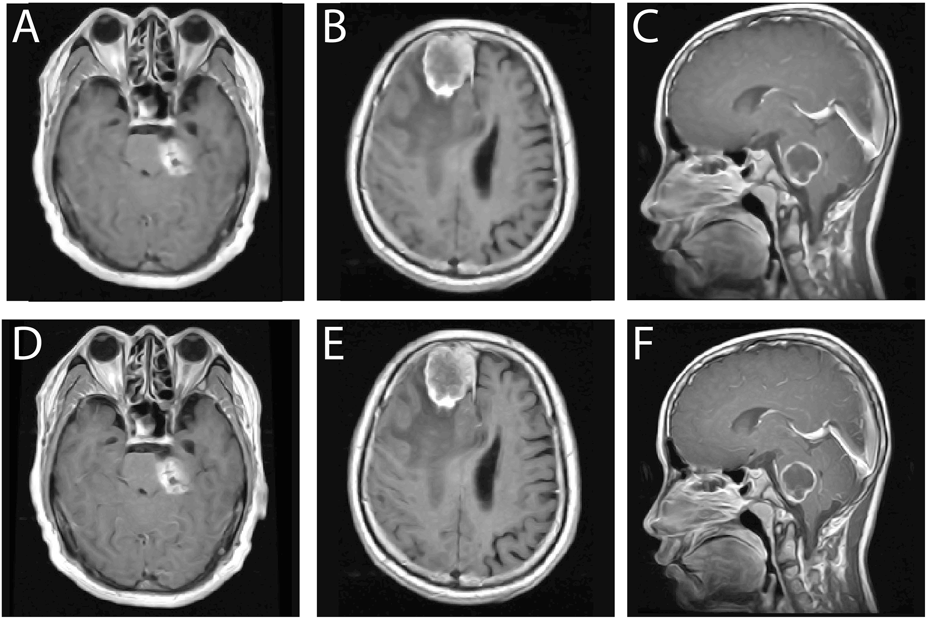
Coherence of brain MRI images
Low contrast in brain MRI scans can obscure important structural variations, which makes tumor localization challenging. For this reason, contrast enhancement is required. After noise removal, certain regions in the MRI remain non coherent, and these inconsistencies make it more difficult to identify tumor boundaries accurately. Multiple areas within a single scan may exhibit weak coherence, and to address this issue, oriented diffusion filtering is applied as an initial step in the coherence enhancement process. This technique requires orientation information from local image regions, known as the orientation field (OF), which guides the diffusion tensor to follow the correct direction for maintaining detail consistency in the image (Soomro et al., 2021). Identifying the most coherent region within the scan is essential because it enables a clearer visualization of fine structural details that support reliable tumor detection.
To achieve a coherent representation of brain MRI images, we adopted the optimization scheme of the Anisotropic Diffusion Filter (Gottschlich & Schönlieb, 2012; Alqahtani Saeed et al., 2023). The method involves the following steps:
-
1.
Compute the second moment matrix for each pixel in the MRI region.
-
2.
Assign a diffusion matrix to every pixel, ensuring region specific diffusion behavior.
-
3.
Determine the intensity variation for each pixel using the following expression: .
-
4.
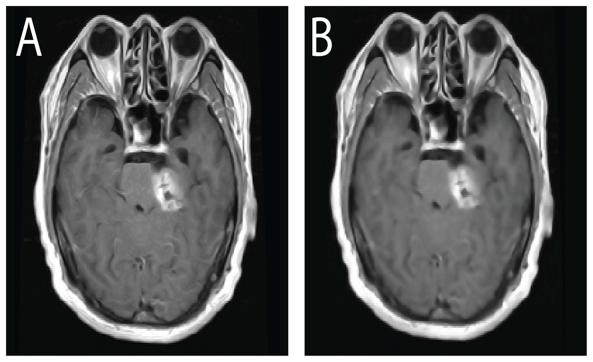
Figure 5: Effect of CLAHE on brain MRI scans.
(A) Original low contrast MRI where tumor regions blend with surrounding tissue, reducing visibility. (B) CLAHE enhanced image showing improved local contrast, clearer tissue separation, and more distinct tumor boundaries, which supports accurate segmentation and classification.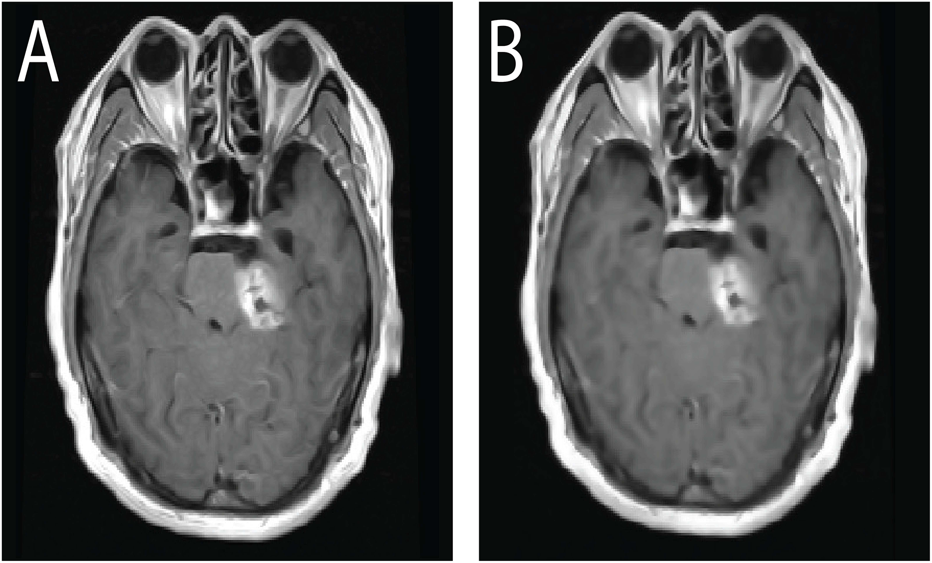
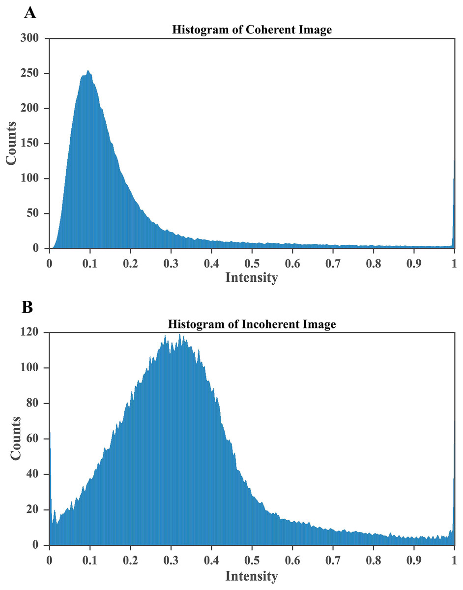
Figure 6: CLAHE based enhancement of brain MRI intensity distribution.
(A) Histogram after applying CLAHE showing a broadened and balanced intensity spread that improves contrast and enhances visibility of structural details. (B) Histogram of the original MRI image with pixel intensities concentrated in the lower range, indicating poor contrast and limited tissue differentiation. The improved contrast in (A) enables clearer identification of tumor regions, which is essential for accurate segmentation and diagnosis.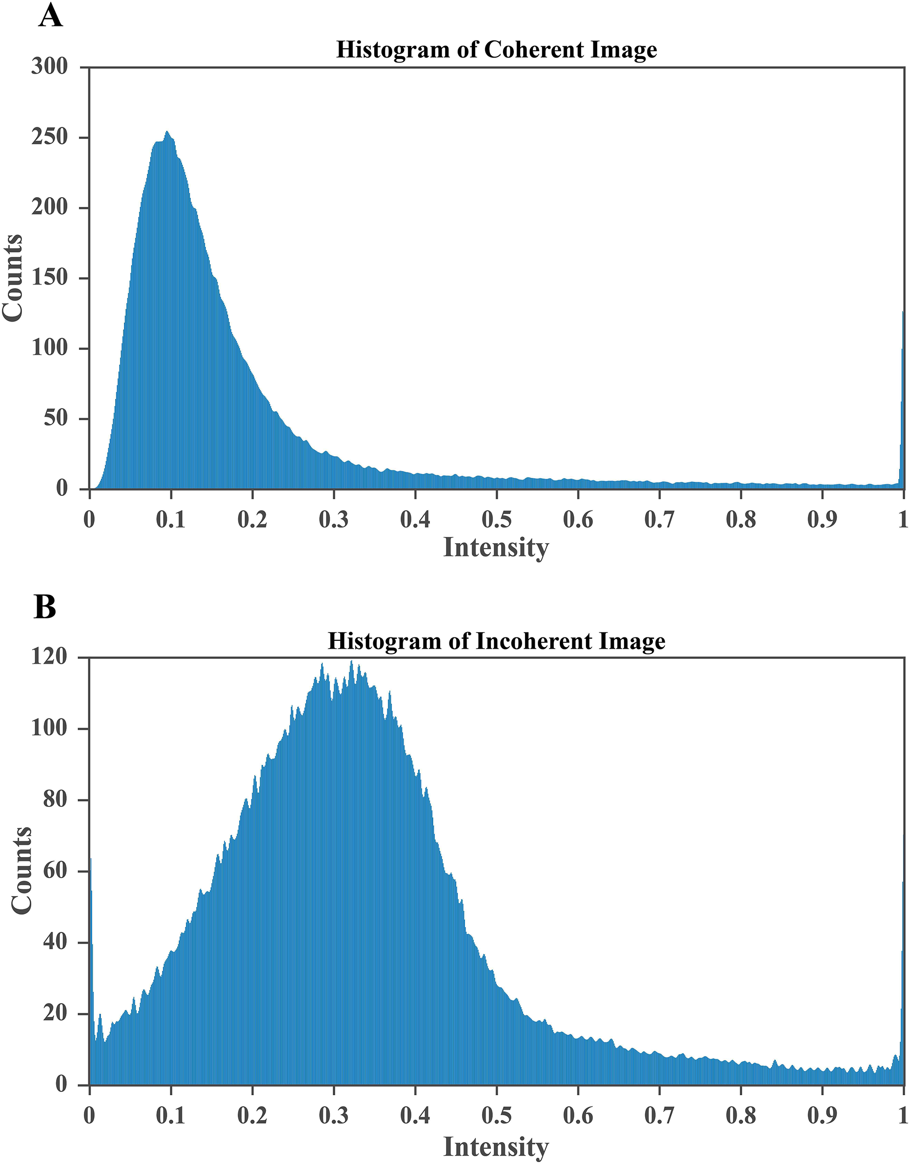
Contrast enhancement of brain MRI scans
To improve the visualization of localized tumor features in brain MRI images, Contrast Limited Adaptive Histogram Equalization (CLAHE) is applied. CLAHE operates on small contextual tiles rather than on the entire image, which allows local contrast enhancement while controlling the amplification of noise (Mgbejime et al., 2022). This makes it particularly suitable for highlighting tumor regions that often appear within confined and low contrast areas of brain scans. By enhancing subtle local intensity variations, CLAHE improves tissue contrast and preserves important structural details without introducing undesirable artifacts. The method adaptively adjusts contrast within each tile and then blends the processed regions in a smooth manner to generate the final enhanced output. A representative example of CLAHE applied to a sagittal CE MRI scan is presented in Fig. 7. The mathematical formulation and implementation procedure for CLAHE are provided in ‘CLAHE Algorithm and Contrast-Limiting Function’.
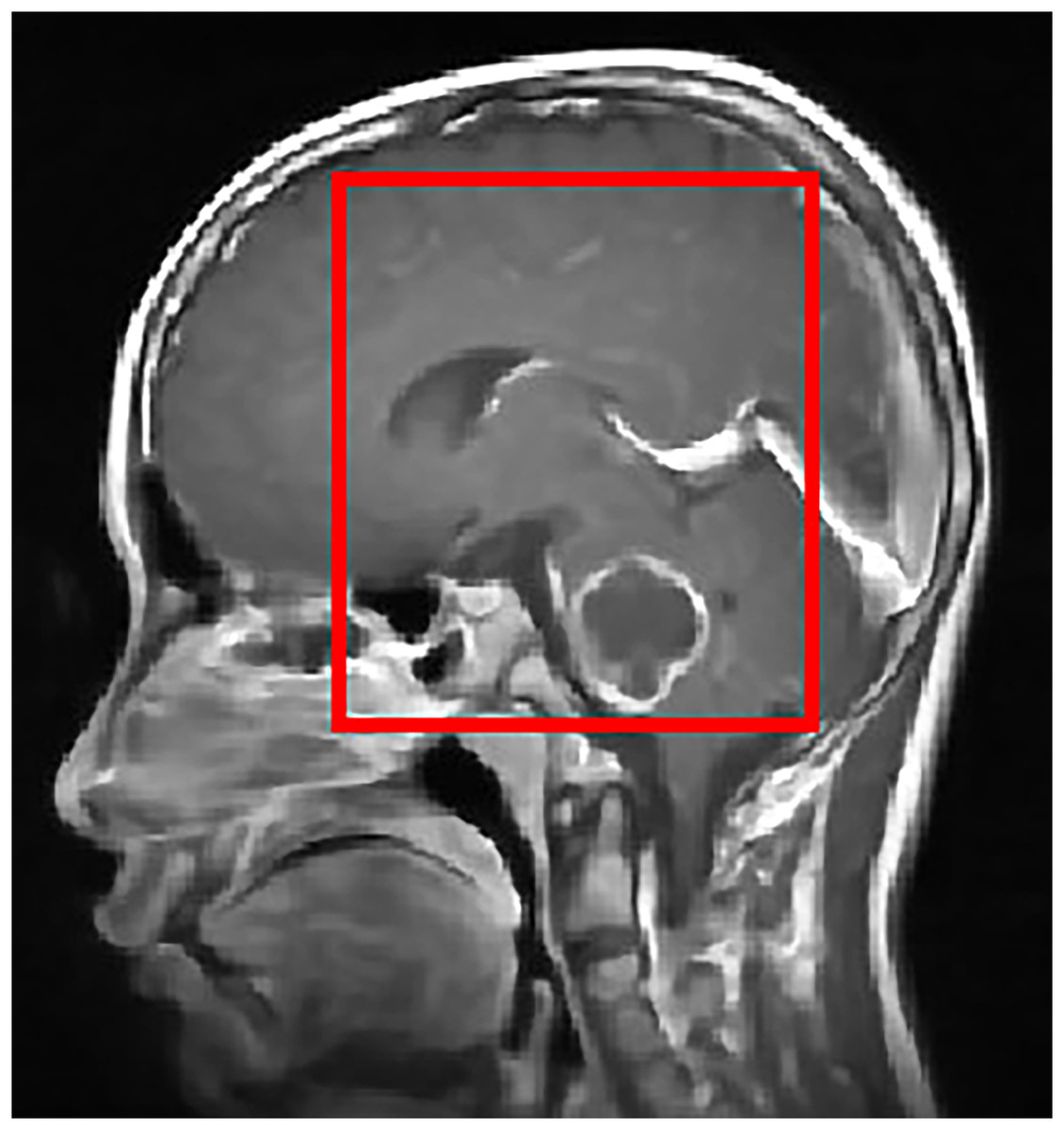
Figure 7: Output of CLAHE applied to a sagittal T1 weighted CE MRI scan. The red bounding box shows the ROI where tumor visibility is enhanced.
CLAHE increases local contrast and improves edge definition, especially in regions with subtle intensity changes, which helps in tissue differentiation and clearer tumor boundary detection. This preprocessing step supports the segmentation and classification stages by enhancing structural clarity in diagnostically relevant areas.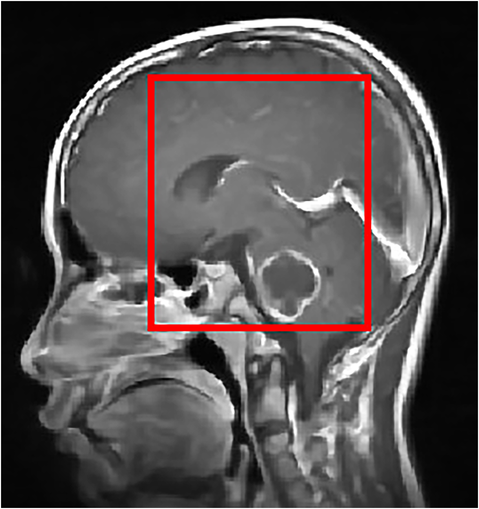
Once contrast is enhanced, the image is binarized using thresholding to isolate potential tumor regions.
Post-processing: segmentation of brain tumor region
Accurate segmentation is a crucial step in medical image analysis because it enables the precise isolation of tumor regions that support diagnosis and treatment planning. In this study, we employ the Fast Marching Method (FMM) due to its reliability, computational efficiency, and suitability for medical imaging tasks. The Fast Marching Method, introduced by James Sethian, provides a strong numerical framework for analyzing boundary evolution in images and signals. It is grounded in well established mathematical principles and has been widely used in applications such as image processing, pattern recognition, and surface extraction. The method also shares conceptual similarities with the level set approach, which has been applied extensively in various image analysis problems (Sethian, 1999).
In this work, the Fast Marching Method is utilized to address the challenging task of brain tumor segmentation in MRI scans. Its propagation based mechanism allows the algorithm to move through the image in a controlled manner that follows local intensity variations, which helps in identifying coherent boundaries that approximate the tumor region. Successful application of FMM requires an understanding of the speed function, propagation rules, and the behavior of the evolving front as it interacts with anatomical structures. The following sections describe the complete procedure used in this study, detailing how FMM is applied to MRI brain images to obtain accurate and consistent segmentation of tumor regions.
Mathematical formulation of FMM
The FMM models front propagation based on the Eikonal equation, formulated as:
(2) where represents the arrival time of the expanding front at a point and is the speed function controlling the propagation rate over the computational domain . The initial condition is defined as:
(3) where represents the seed region from which expansion begins.
FMM iteratively calculates the arrival times at each point in , ensuring the front propagates smoothly until it converges at the desired boundary. This makes it highly effective in brain tumor segmentation, where the evolving interface accurately delineates the tumor based on intensity variations.
The segmentation approach integrates FMM with the Level Set Method, where a deformable contour is represented by a static level-set function. The governing equation for this evolution is:
(4)
This formulation consists of three primary computational steps:
-
1.
Speed function calculation
-
The velocity of the evolving contour is computed based on the image gradient, which determines the strength of movement:
(5)
-
-
2.
Smoothing for boundary enhancement
A Gaussian filter is applied to refine the image and enhance boundary localization. The term accounts for curvature effects, while directs the front toward the object boundary.
-
3.
Contour evolution for tumor segmentation: The tumor segmentation is conducted in two steps:
-
FMM is used to evolve the contour:
(6)
(7)
Once segmentation is complete, Eq. (4) is solved using the computed boundary conditions, ensuring precise detection of the tumor. The results are depicted in Fig. 8, illustrating the effectiveness of the proposed approach.
-
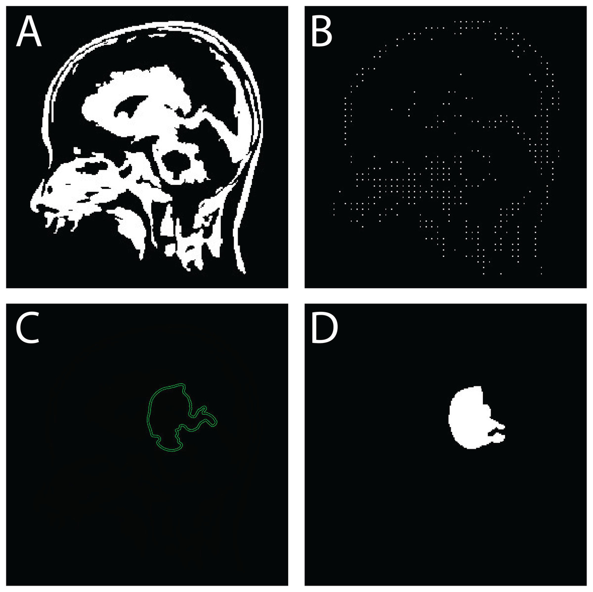
Figure 8: Sequential outputs of the SVM-based brain tumor classification framework: (A) binary segmentation map highlighting tumor regions post-initial processing, (B) skeletonized representation preserving structural topology for handcrafted feature extraction, (C) predicted tumor region generated by the SVM classifier, and (D) final delineated tumor contour for diagnostic interpretation.
These stages reflect the modular progression from segmentation to classification and delineation within the proposed FMM-SVM pipeline.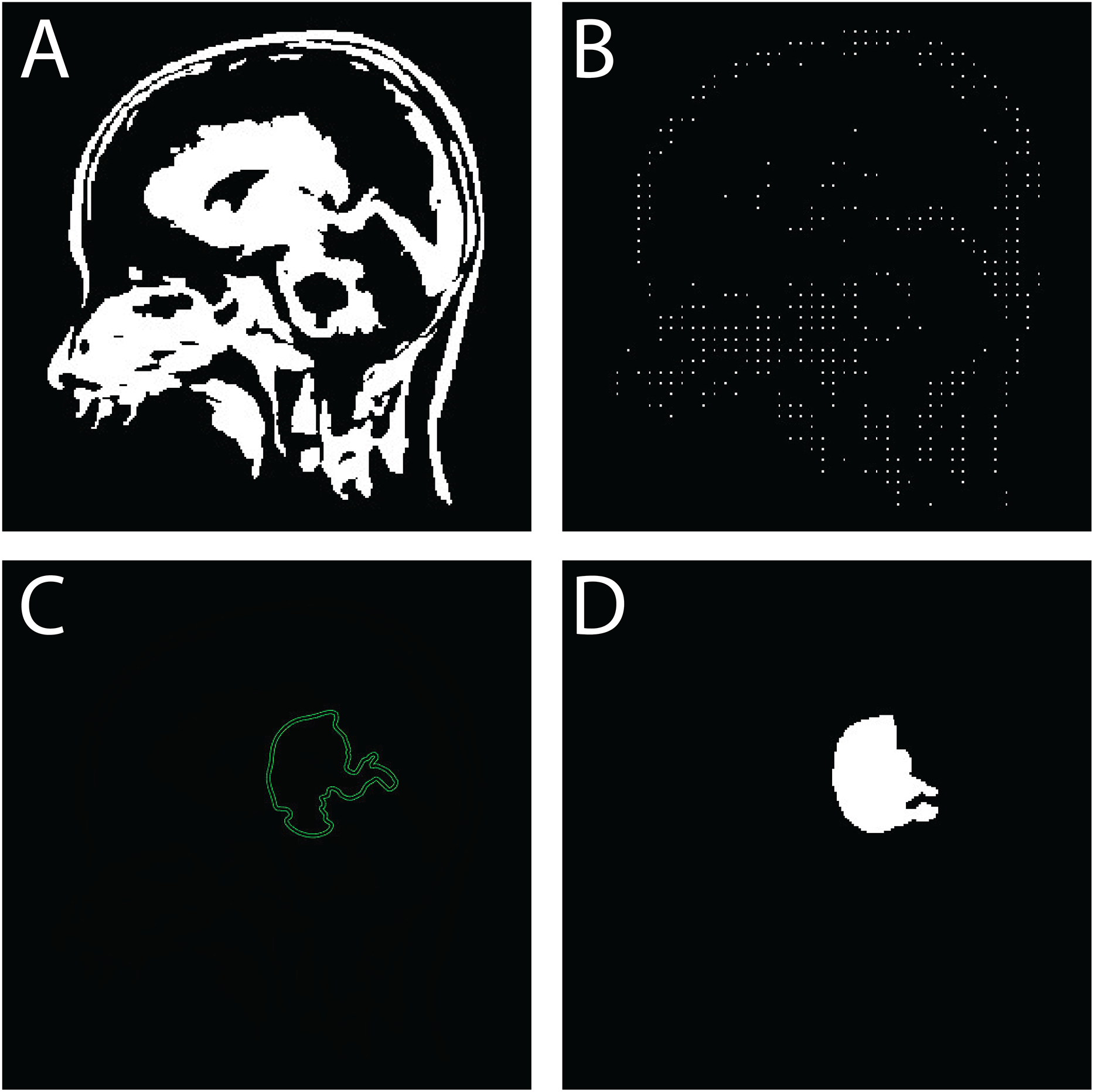
The following pseudo-codes outline the algorithmic steps for brain tumor segmentation using the FMM and Level Set-Based Contour Evolution.
Algorithmic implementation for brain tumor segmentation: The following pseudo-codes outline the algorithmic steps for brain tumor segmentation using the FMM (please refer to Algorithm 1) and Level Set-Based Contour Evolution (please refer to Algorithm 2).
| Require: MRI Image , Seed Point |
| Ensure: Segmented tumor region |
| 1: Initialization |
| 2: Set seed point with zero arrival time |
| 3: Initialize priority queue (min-heap) and mark all pixels as unprocessed |
| 4: Speed Function Computation |
| 5: Compute speed function based on image gradients |
| 6: Front Propagation |
| 7: while priority queue is not empty do |
| 8: Extract point with smallest arrival time |
| 9: Update arrival times for neighboring pixels |
| 10: Insert updated neighbors into the priority queue |
| 11: end while |
| 12: Output |
| 13: Return segmented tumor region |
| Require: Initial tumor segmentation from FMM, Image |
| Ensure: Refined tumor boundary |
| 1: Initialization |
| 2: Define level-set function with inside tumor and outside |
| 3: Compute Evolution Terms |
| 4: Compute gradient and curvature term |
| 5: Compute velocity function |
| 6: Contour Evolution |
| 7: while Convergence not reached do |
| 8: Update level set function using: |
| 9: |
| 10: end while |
| 11: Output |
| 12: Return final tumor boundary |
FMM is employed in this study because of its strong capability to segment complex anatomical structures while maintaining a low computational workload. The method produces accurate contour progression by efficiently solving the Eikonal equation, which provides a well structured approach for boundary tracking without the need for reinitialization or iterative energy minimization. Traditional level set methods often encounter computational challenges, particularly when handling topological changes or weak boundary gradients. In contrast, FMM offers improved numerical stability and faster performance, making it highly suitable for images that contain heterogeneous intensity patterns, such as brain tumor regions in MRI scans. Level set based techniques may drift or overfit in areas with limited contrast, whereas FMM adapts its propagation behavior to local spatial variations, ensuring boundary consistency throughout the segmentation process. This degree of reliability, combined with its reduced processing cost, makes FMM a practical and scalable choice for clinical workflows where precision, robustness, and efficiency are essential.
SVM-based tumor classification framework
Following segmentation, the identified tumor regions must be classified to distinguish abnormal tissue from healthy areas. In this stage, SVM is used for accurate categorization. The final component of the proposed brain tumor detection pipeline employs a SVM classifier to reliably separate tumor regions from non tumor regions based on the extracted features. SVM is a well established supervised learning technique widely applied in medical image analysis because of its ability to construct an optimal separating hyperplane that maximizes class distinction and supports precise decision making (Vankdothu & Hameed, 2022).
Dataset representation and classification objective: The annotated dataset used for training is represented as:
(8) where denotes the feature vector derived from the preprocessed MRI scan, and is its corresponding binary label: for tumor and for non-tumor.
The goal of the SVM is to learn a classification function such that:
(9) with maximum margin and minimal misclassification.
Hinge loss and decision boundary: The optimization process in SVM relies on the hinge loss function:
(10) which imposes zero loss for correctly classified points lying outside the margin and a linear penalty for those misclassified or within the margin. This loss formulation encourages maximum margin separation while minimizing classification error.
The decision function used for classification is:
(11) where are Lagrange multipliers, are labels, are support vectors, is the test sample, is the kernel function, and is the bias.
Kernel Selection: This study employs the Radial Basis Function (RBF) kernel due to its capacity to model nonlinear decision boundaries, which are often present in brain tumor data. The RBF kernel is defined as:
(12) where is a hyperparameter controlling the width of the Gaussian kernel. The RBF kernel demonstrated better classification performance than linear and polynomial kernels based on empirical evaluation.
Classification pipeline: The classification process consists of the following stages:
Feature extraction: Key features that describe texture, intensity, shape, and topological characteristics are computed from the segmented and skeletonized images. A total of 100 features are extracted and organized into four major groups. Intensity features such as mean, variance, and skewness characterize pixel value distributions within the tumor region. Texture features derived from the Gray Level Co occurrence Matrix (GLCM) and Local Binary Patterns (LBP) capture spatial relationships and local variations in tissue structure. Shape descriptors, including area, eccentricity, and solidity, help summarize the geometry of the tumor. Topological features such as the Euler number and skeleton length provide information about structural complexity. These features are selected due to their established relevance in brain tumor analysis and are refined using correlation filtering to retain the most informative and non redundant variables.
Model training: The SVM classifier is trained using the extracted features along with labeled data so that it can learn optimal decision boundaries that separate tumor from non tumor regions.
Prediction: Once the model is trained, it is applied to new MRI scans to classify regions of interest as tumor or non tumor based on the learned decision function.
Figure 8 presents a visual example of the SVM based classification workflow, illustrating the final stage of the detection pipeline. This produces a clinically interpretable output with clearly delineated tumor regions, which supports accurate diagnostic decision making.
Algorithmic implementation The complete classification process is summarized in Algorithm 3.
| Require: Feature dataset with |
| Ensure: Trained SVM model and tumor predictions |
| 1: Convert MRI images to grayscale and denoise using FMM segmentation |
| 2: Extract features: shape, intensity, texture |
| 3: Select RBF kernel and train SVM model |
| 4: for each new feature vector x do |
| 5: Compute decision function |
| 6: Assign class label |
| 7: end for |
| 8: Return tumor classification results |
SVM optimization and training strategy
To ensure reproducible and reliable classification results, a structured optimization strategy was applied to the Support Vector Machine (SVM) model. The classification stage was built around the RBF kernel, which was selected because of its strong capacity to handle non linear decision boundaries that commonly arise in feature spaces derived from brain MRI scans. Initial experimentation showed that the RBF kernel provided more stable and accurate performance compared with linear and polynomial kernels, particularly when dealing with heterogeneous feature distributions. This consistency made the RBF kernel the most suitable choice for the classification framework used in this study.
Hyperparameter Selection: Two principal hyperparameters, the regularization parameter C and kernel coefficient , were tuned using a grid search technique. This involved evaluating model performance over a parameter grid:
.
Each combination of C and was assessed to identify the optimal configuration that balances margin maximization and generalization.
Cross-Validation Framework: A 10-fold stratified cross-validation approach was adopted to ensure statistical robustness and class balance. The dataset was partitioned into ten equally sized subsets, maintaining consistent tumor and non-tumor ratios across folds. For each fold, the model was trained on nine partitions and validated on the remaining one. This procedure was repeated iteratively, and the final model performance was derived from the averaged results across To ensure robust evaluation and minimize bias due to dataset partitioning, we employed stratified -fold cross-validation with . This technique maintains the proportional distribution of tumor classes (glioma, meningioma, and pituitary) across all folds, ensuring balanced representation in both training and testing subsets. Each fold involved training on four partitions and testing on the remaining one, cycling through all combinations to compute average performance metrics. This stratification is particularly important given the class imbalance within the CE-MRI dataset. Performance metrics, including Dice Similarity Coefficient, Jaccard Index, accuracy, sensitivity, and specificity, were averaged over the five folds, with standard deviation reported to capture variability. This approach enhances the statistical reliability and generalizability of the reported results.
Evaluation Metrics: The grid search optimization was guided by multiple performance indicators, including classification accuracy, Dice Similarity Coefficient (DSC), sensitivity, and specificity. The parameter combination yielding the highest average performance across folds was selected as the final model configuration. This comprehensive training and tuning strategy enhances model reliability, promotes generalizability across unseen data, and ensures methodological transparency for future replication.
To ensure transparent and reproducible optimization, the hyperparameters of the SVM classifier were tuned through a structured grid-search procedure. The regularization constant C was varied across a logarithmic range from to , while the kernel width was explored over a comparable interval to evaluate the non-linear separability of the feature space. Training and validation curves were generated to identify the region where the validation accuracy stabilizes without signs of overfitting. The optimal configuration was obtained at and , providing an effective balance between margin flexibility and generalization capability. The validation trend shown in Fig. 9 illustrates this behavior, where performance improves up to the optimal range and declines thereafter due to overfitting. This optimization strategy ensures that the final SVM model remains stable, well-calibrated, and suitable for accurate tumor classification.
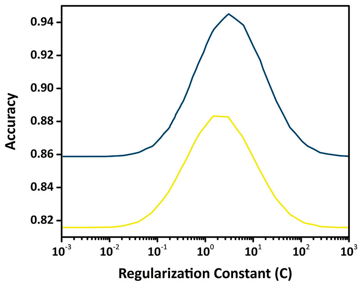
Figure 9: Validation curve for the SVM classifier showing training and validation accuracy across different values of the regularization constant (C) using an RBF kernel.
The optimal value of C is identified where validation accuracy peaks, indicating the best trade-off between margin maximization and misclassification penalty.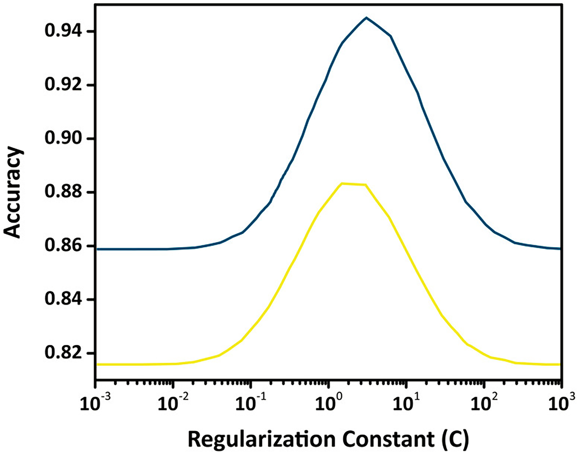
Composed algorithm
The proposed algorithm introduces a comprehensive and robust strategy for detecting brain tumors by addressing core challenges in MRI analysis, including noise suppression, contrast enhancement, and accurate classification. The full workflow is presented in Fig. 10.
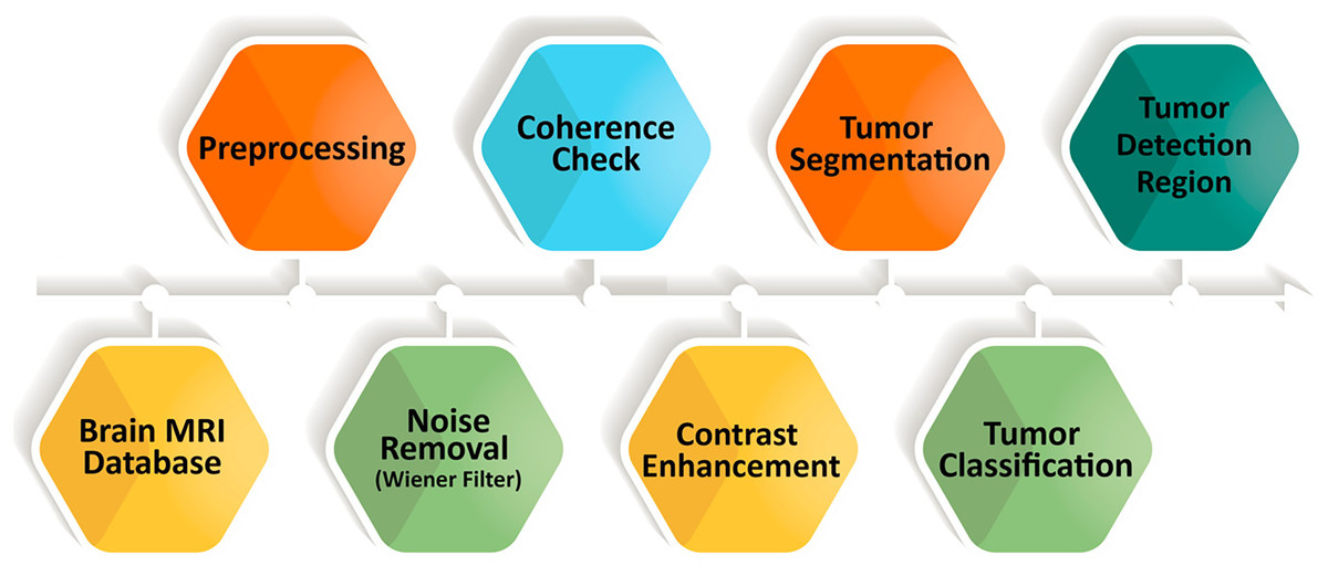
Figure 10: Enhanced brain tumor detection algorithm, a comprehensive workflow for accurate analysis of MRI images.
A major difficulty in MRI based tumor detection is the presence of noise and uneven contrast across brain regions, which can obscure important anatomical details and reduce segmentation accuracy. To overcome these issues, the algorithm incorporates a multi stage enhancement process that includes Wiener filtering for noise reduction, followed by oriented diffusion filtering and CLAHE for contrast improvement. This preprocessing sequence refines the visual quality of MRI scans and prepares them for more reliable downstream analysis.
After enhancement, the FMM is applied to perform precise tumor segmentation. This step is essential for obtaining accurate boundary delineation while preserving critical structural information, which improves the reliability of the segmentation output. The extracted tumor regions are then used to compute descriptive features that form the basis of the classification stage.
For classification, the algorithm employs the Support Vector Machine (SVM), a model widely recognized in medical imaging for its strong performance in binary decision tasks. With optimized kernel selection and parameter tuning, the SVM effectively distinguishes tumor regions from non tumor regions and reduces the occurrence of false detections.
Empirical evaluations show that the proposed framework achieves superior performance compared with conventional approaches in terms of accuracy and computational efficiency. The integrated pipeline, which combines enhancement, segmentation, and classification, not only improves diagnostic precision but also maintains fast processing times, making the method suitable for real time clinical workflows. Furthermore, the algorithm demonstrates consistent and reliable performance across different MRI scans, reinforcing its relevance in automated tumor detection.
In conclusion, the proposed system successfully addresses the limitations of existing methods by integrating advanced preprocessing, precise segmentation, and optimized classification. Its ability to improve MRI quality, maintain computational efficiency, and enhance classification accuracy highlights its value in medical image analysis and supports its potential for assisting clinical decision making.
Computational environment
To evaluate the real-time feasibility of the proposed FMM–SVM framework, a detailed runtime assessment was conducted. All experiments were performed on a system equipped with an Intel Core i7 CPU, 32 GB RAM, and Windows 11 OS. The entire implementation was carried out in MATLAB R2023a using the Image Processing Toolbox (IPT) and Statistics and Machine Learning Toolbox (SMLT).
The runtime was averaged across 100 CE-MRI brain images, covering all stages of the pipeline, including preprocessing, segmentation with the FMM, feature extraction, and classification using SVM. The average execution time was approximately 0.43 s per image, confirming the framework’s suitability for near real-time medical applications.
These results demonstrate that the method achieves high performance without relying on high-end GPU hardware, making it practical for use in resource-limited clinical environments.
Evaluation proposed
The effectiveness of the proposed FMM-SVM approach is determined by evaluating both the segmentation of brain tumor regions and the classification outcomes. For segmentation evaluation, six statistical descriptors are employed: skewness, kurtosis, entropy, contrast, standard deviation, and mean to analyze texture and intensity-based characteristics. For classification, model performance is assessed through accuracy, specificity, and sensitivity derived from confusion matrix-based evaluation.
Measuring parameters: segmentation of brain tumor
The segmentation quality is quantitatively evaluated using six metrics: skewness, kurtosis, entropy, contrast, standard deviation, and mean. These descriptors capture the statistical and spatial complexity of the segmented tumor regions, offering insights into textural heterogeneity and contrast variations. Detailed definitions and roles of these metrics are referenced from Almalki et al. (2022).
Measuring parameters: classification of brain tumor
Classification performance was measured using both training and testing datasets. To ensure robust and unbiased evaluation, k-fold cross-validation (k = 10, stratified) was applied. The classification metrics include accuracy, specificity, and sensitivity, which were computed based on confusion matrix outputs. In addition, segmentation-informed classification was evaluated using Dice Similarity Coefficient (DSC), Hausdorff Distance (HD), and Jaccard Similarity Index (JSI). All mathematical formulations of the above evaluation parameters, Confusion Matrix, Sensitivity, Specificity, Accuracy, DSC, HD, and JSI—are comprehensively explained in ‘C: Evaluation Metrics Formulations’.
Results and discussion
This section presents a detailed evaluation of the proposed FMM-SVM framework, covering its impact on preprocessing, denoising, segmentation, classification, and comparative performance with existing methods.
Impact of pre-processing
Preprocessing plays a crucial role in improving MRI quality, directly influencing segmentation accuracy and classification reliability. By refining image contrast, reducing noise, and preserving anatomical structures, preprocessing enhances the clarity of tumor boundaries, leading to more precise feature extraction and classification. CLAHE and diffusion filtering significantly improve image quality by enhancing contrast and structural integrity, ensuring better differentiation between normal and abnormal tissues. Additionally, Wiener filtering outperforms conventional denoising techniques, maintaining critical tumor structures while effectively suppressing noise.
Quantitative evaluation of preprocessing impact
To evaluate the effectiveness of preprocessing, various quality metrics were computed, demonstrating its substantial impact on image enhancement. CLAHE significantly increases contrast, improving CNR from 2.4 to 4.1, which helps distinguish tumor regions more effectively. The entropy of processed images also increases from 5.21 to 6.15, indicating improved information retention and enhanced visualization of fine structures. Diffusion filtering enhances SSIM from 0.68 to 0.88, ensuring smoother intensity transitions while maintaining the integrity of anatomical features. The combination of CLAHE and diffusion filtering achieves the best overall enhancement, with PSNR reaching 34.1 dB and SSIM improving to 0.91, reinforcing its effectiveness in preprocessing. Table 1 summarizes the quantitative impact of preprocessing techniques.
| Preprocessing method | PSNR (dB) | SSIM | CNR | Entropy |
|---|---|---|---|---|
| Original image | 27.10 | 0.680 | 2.40 | 5.21 |
| CLAHE | 30.50 | 0.820 | 4.10 | 6.15 |
| Diffusion filtering | 32.30 | 0.880 | 4.80 | 6.47 |
| CLAHE + Diffusion filtering | 34.10 | 0.910 | 5.20 | 6.83 |
The results confirm that applying CLAHE and diffusion filtering significantly enhances image contrast, reduces noise, and improves structural clarity, leading to better segmentation accuracy and improved tumor detection.
Comparative analysis of Wiener filtering vs. other denoising methods
Denoising is essential to maintain the integrity of tumor structures while reducing noise-induced artifacts in MRI images. Various denoising techniques were compared, highlighting the superiority of Wiener filtering over Gaussian, median, and bilateral filtering. Gaussian filtering exhibits moderate performance in edge preservation but leads to blurring effects that reduce segmentation accuracy. Median filtering effectively retains edges but offers limited noise suppression. Bilateral filtering balances noise reduction and structure preservation, yet Wiener filtering achieves the highest PSNR (33.5 dB) and SSIM (0.89), demonstrating optimal noise suppression with minimal structural distortion. Table 2 presents the comparative performance of different denoising techniques.
| Denoising method | PSNR (dB) | SSIM | Edge preservation | Noise reduction |
|---|---|---|---|---|
| Gaussian filtering | 29.40 | 0.760 | Moderate | Low |
| Median filtering | 28.90 | 0.740 | High | Moderate |
| Bilateral filtering | 31.20 | 0.810 | High | Moderate |
| Wiener filtering | 33.50 | 0.890 | Very high | High |
The findings indicate that Wiener filtering effectively reduces noise while preserving essential details, unlike Gaussian filtering, which smooths the image but compromises critical features. Median and bilateral filtering offer moderate improvements but lack the robustness of Wiener filtering, making the latter the preferred denoising method for medical imaging applications.
Empirical justification for preprocessing sequence
To justify the specific order of preprocessing operations—namely, Wiener filtering followed by oriented diffusion filtering and finally CLAHE a comparative analysis was performed by altering the sequence of these steps. The impact of each configuration was assessed in terms of segmentation accuracy using key evaluation metrics such as DSC, (JSI, and HD). Results are summarized in Table 3.
| Preprocessing sequence | DSC (%) | JSI (%) | HD (pixels) |
|---|---|---|---|
| Wiener Diffusion CLAHE (Proposed) | 96.3 | 89.5 | 3.12 |
| CLAHE Wiener Diffusion | 91.8 | 84.2 | 4.17 |
| Diffusion CLAHE Wiener | 93.1 | 85.7 | 4.00 |
| No preprocessing | 86.5 | 78.2 | 5.21 |
The proposed sequence, beginning with Wiener filtering, provided the highest segmentation accuracy. Initiating preprocessing with Wiener filtering effectively reduced baseline noise while preserving anatomical structures. Subsequent application of diffusion filtering improved edge continuity, and final contrast enhancement via CLAHE helped delineate tumor boundaries more distinctly. In contrast, reversing the order (e.g., applying CLAHE first) amplified noise artifacts, which degraded segmentation quality.
Analysis of segmentation module
Accurate segmentation is fundamental for reliable tumor detection, influencing both classification and diagnostic precision. The performance of the segmentation module is assessed using the CE-MRI dataset, where statistical measures quantify improvements in contrast, structure preservation, and segmentation accuracy. These metrics validate the effectiveness of the proposed approach in delineating tumor boundaries while reducing classification errors.
Segmentation module performance assessment
The quantitative analysis of the segmentation model evaluates its capability to enhance contrast, reduce distortions, and improve tumor boundary definition. The computed statistical values, including skewness, kurtosis, entropy, contrast enhancement, and intensity variations, provide a comprehensive insight into segmentation performance.
Table 4 presents the segmentation results, showing a substantial improvement in contrast across tumor types. Notably, for pituitary tumors, the IC value of 0.030 indicates enhanced differentiation between tumor and non-tumor regions. The increased entropy values across all tumor types confirm improved information retention, essential for identifying subtle variations in tumor structures. The skewness and kurtosis values demonstrate a more uniform intensity distribution, ensuring balanced segmentation results without excessive brightness or dark regions.
| Tumor type | Skewness | Kurtosis | Entropy | IC | STD | Mean |
|---|---|---|---|---|---|---|
| Pituitary tumor | 5.26 | 32.92 | 3.01 | 0.29 | 0.084 | 0.0041 |
| Gliomas tumor | 5.31 | 33.13 | 3.01 | 0.29 | 0.089 | 0.0044 |
| Meningiomas tumor | 5.84 | 35.20 | 3.19 | 0.30 | 0.090 | 0.0046 |
The results confirm that the proposed segmentation method enhances tumor visibility by increasing contrast and entropy while maintaining stable intensity variations. This balance ensures that the model successfully captures fine details without introducing distortions, making segmentation more reliable and interpretable for clinical diagnosis.
Comparative evaluation of FMM with deep learning based segmentation models
To provide a rigorous assessment of the proposed FMM for brain tumor segmentation, a comparative evaluation was performed against two widely used deep learning architectures, U Net and a conventional Convolutional Neural Network (CNN) based segmentation model. All methods were tested on the CE MRI dataset using identical preprocessing steps, which included Wiener filtering and CLAHE based contrast enhancement, to ensure fair and consistent comparison. The quantitative results summarized in Table 5 present the performance across several evaluation metrics, including DSC, JSI, HD, SE, SP, and AC.
| Model | DSC (%) | JSI (%) | HD (pixels) | SE (%) | SP (%) | AC (%) |
|---|---|---|---|---|---|---|
| FMM (Proposed) | 89.56 | 81.92 | 3.12 | 91.44 | 95.62 | 93.10 |
| U-Net | 91.87 | 84.76 | 3.94 | 93.65 | 94.82 | 93.98 |
| CNN-based model | 88.23 | 80.45 | 4.10 | 90.27 | 92.30 | 91.12 |
Note:
Dice, JSI, SE, SP, and AC are expressed in percentage (%). HD is reported in pixels.
As anticipated, U Net achieved the highest DSC and JSI values, demonstrating its strong ability to capture complex spatial patterns and detailed tumor structures. However, this level of accuracy required extensive training, high memory consumption, and noticeably longer inference times. The CNN based model showed reduced segmentation performance, which reflects its limitations in modeling diverse tumor shapes and intensity variations without more advanced architectural components or access to large annotated datasets.
The proposed FMM based approach, although slightly lower than U Net in absolute accuracy, delivered competitive performance while maintaining minimal computational cost and requiring no training. This makes FMM particularly suitable for clinical environments where rapid inference, lower hardware requirements, and high reliability are essential. The balance between accuracy and efficiency confirms the practicality of FMM for real time or resource constrained medical imaging applications.
These findings demonstrate that the proposed FMM-based segmentation offers a compelling trade-off between accuracy and computational efficiency. While deep learning models such as U-Net may be preferable when ample labeled data and high-performance hardware are available, the deterministic nature of FMM renders it advantageous in clinical scenarios that demand real-time processing, interpretability, and scalability without reliance on large-scale model training.
Figure 11 illustrates a direct visual comparison between the proposed FMM-based segmentation output and those generated by widely used deep learning models, U-Net and ResNet, across three CE-MRI examples. Each row presents the original scan, ground truth annotation, and segmentation results produced by the three methods. The FMM approach demonstrates high alignment with the annotated masks, preserving tumor contours and volume with strong consistency. Although U-Net and ResNet perform well, some discrepancies can be observed, particularly in border precision and tumor completeness, where slight over- or under-segmentation is evident. The proposed method, despite not relying on extensive training or deep architectures, delivers localization accuracy comparable to or superior to that of reference masks while maintaining minimal deviation from them. This figure reinforces the earlier metric-based findings and visually confirms the reliability of the FMM-based pipeline in capturing diverse tumor shapes and sizes, supporting its viability for use in clinical environments with limited computational resources.
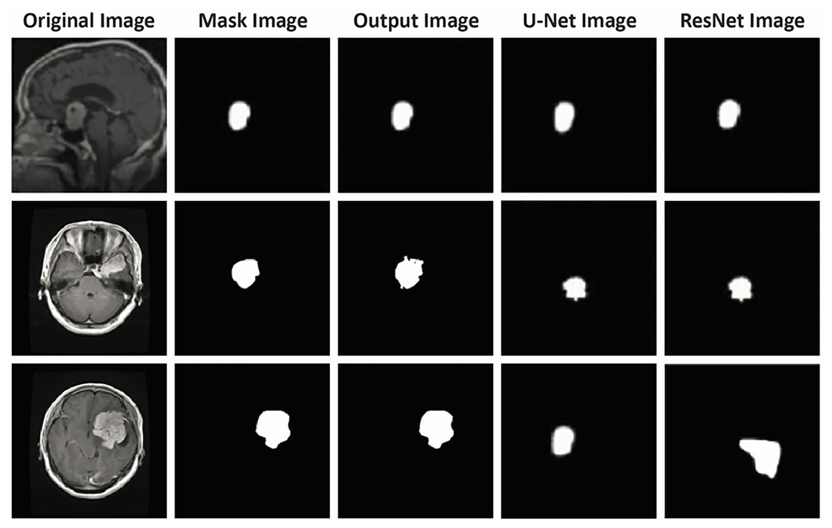
Figure 11: Visual comparison of segmentation outputs. Each row presents a different case: (1) original CE-MRI slice, (2) ground truth mask, (3) output from the proposed FMM-based method, (4) output from U-Net, and (5) output from ResNet-based segmentation.
The proposed FMM approach yields segmentation masks closely aligned with the ground truth, demonstrating comparable or superior performance to U-Net and ResNet in terms of boundary precision and tumor coverage. This qualitative assessment further supports the reported quantitative results, verifying that the FMM-SVM framework maintains accuracy while offering lower computational complexity.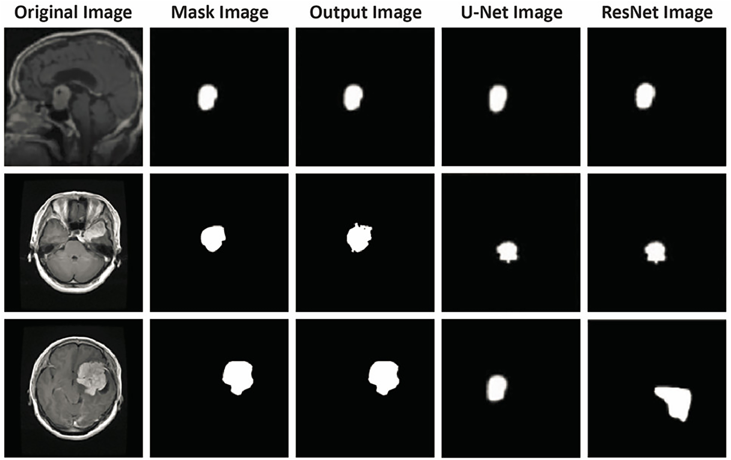
Qualitative validation of segmentation performance
To further validate the segmentation results, a visual comparison between the original MRI images, expert-annotated ground truth masks, and the segmentation outputs is presented in Fig. 12. The first column represents the original MRI scans, the second column contains expert-annotated ground truth masks, and the third column showcases the automated segmentation output generated by the proposed method.
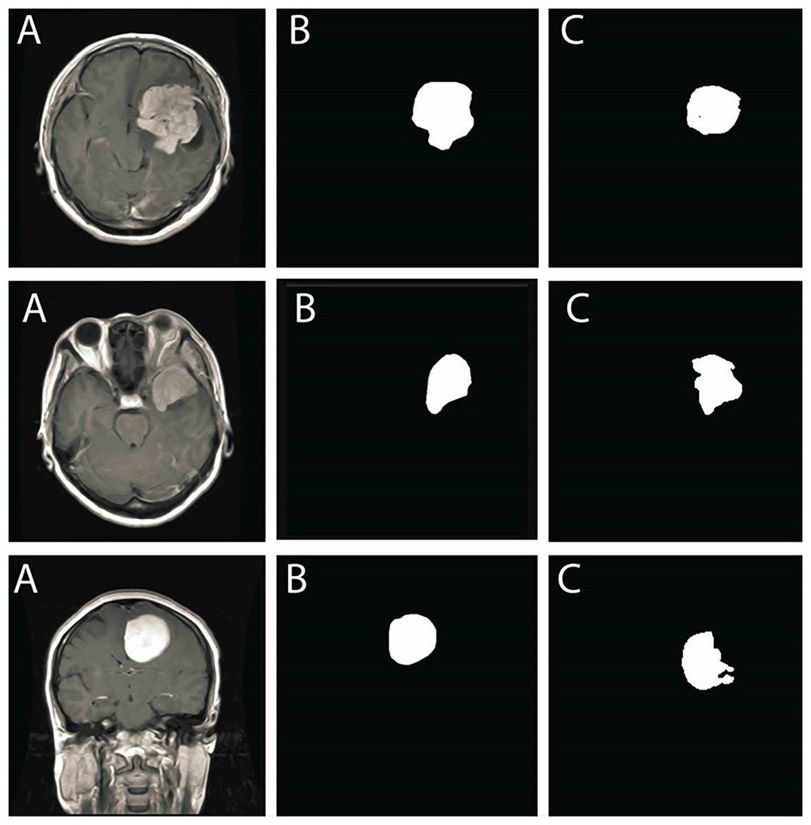
Figure 12: Comparison of segmentation performance: (A) Original MRI scans, (B) Ground truth annotations, (C) Segmentation results obtained using the proposed method.
The results show strong alignment with expert annotations, reinforcing segmentation accuracy.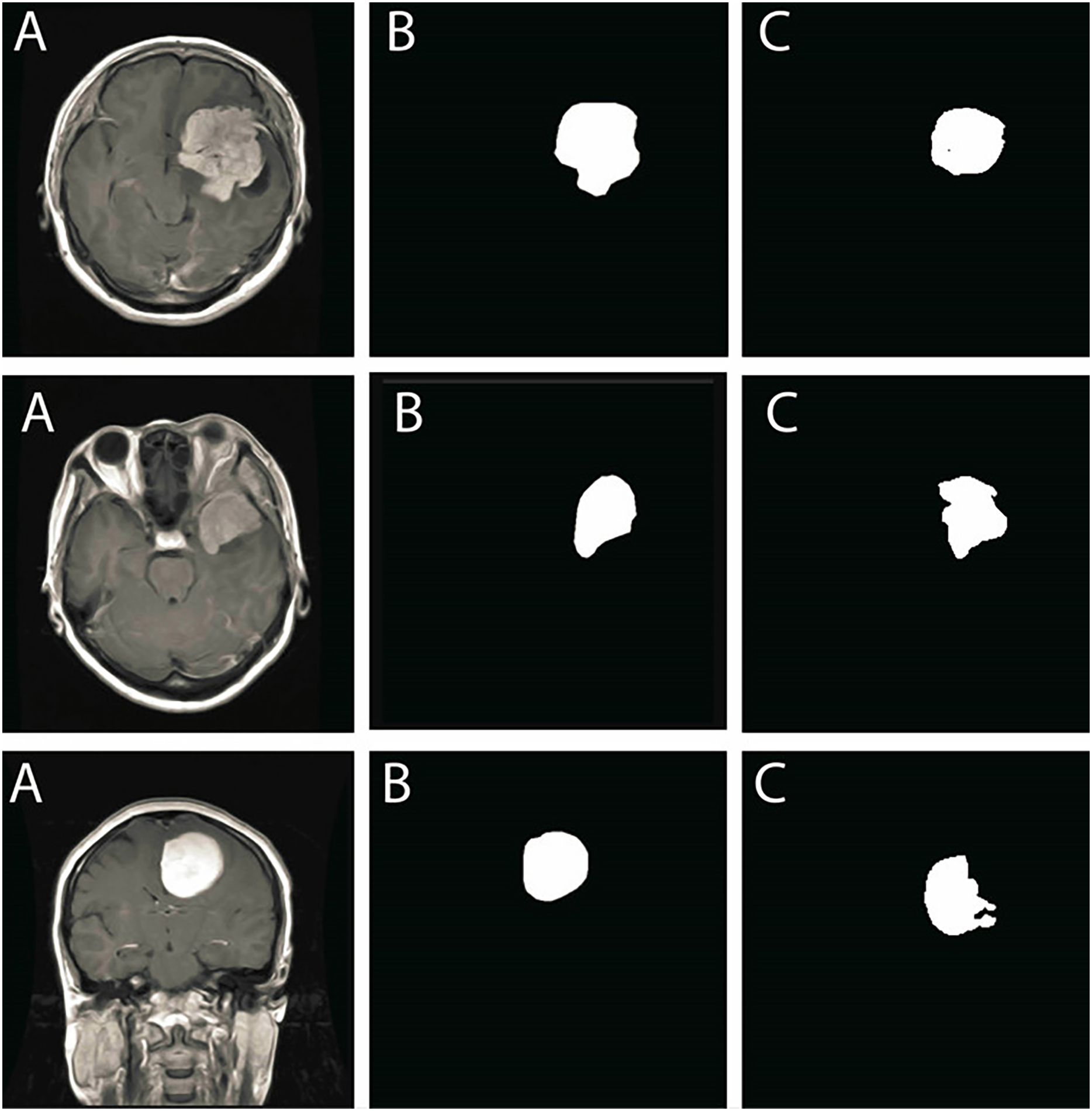
The segmentation results align closely with ground truth annotations, confirming that the model accurately delineates tumor boundaries with minimal discrepancies. The smooth contours of segmented tumor regions further demonstrate that the method efficiently mitigates segmentation inconsistencies, such as excessive fragmentation or over-segmentation.
The qualitative results demonstrate high segmentation precision, reinforcing that the proposed method effectively isolates tumor structures while preserving important tissue details. The consistency across different tumor types highlights the model’s robustness in handling various MRI intensity distributions and complex anatomical structures.
Analysis of classification module
The classification module plays a crucial role in brain tumor detection, distinguishing between different tumor types with high accuracy. The proposed FMM-SVM framework is evaluated on the CE-MRI dataset, and its performance is analyzed using multiple metrics, including sensitivity, specificity, accuracy, DSC, HD, and JSI. The results confirm the robustness and efficiency of the model in accurately classifying brain tumors, maintaining consistency across different tumor types.
Classification module performance assessment
The quantitative evaluation of the classification model demonstrates strong predictive capability, with high sensitivity and specificity values, ensuring a low false-positive and false-negative rate. The DSC values indicate substantial overlap between predicted and actual tumor regions, with an overall DSC of . A one-way ANOVA test confirms no significant variation in DSC scores across tumor types , reinforcing the stability of the classification performance.
To assess the generalization performance of the proposed classification model and validate the application of regularization techniques, we monitored training and validation accuracy across multiple epochs. Figure 13 presents the learning curves over 50 training epochs.
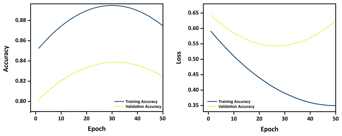
Figure 13: Learning curves showing training and validation accuracy over 50 epochs.
The close alignment between the curves indicates minimal overfitting and strong generalization.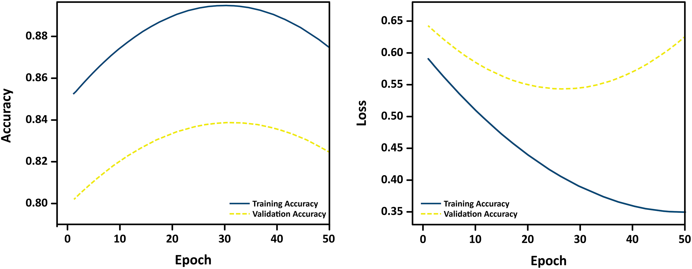
The curves reveal a consistent upward trend in both training and validation accuracy, with minimal divergence, suggesting that the model does not overfit to the training data. The use of L1/L2 regularization, dropout, and early stopping contributed to stabilizing learning and ensuring robust performance on unseen MRI samples. These empirical results confirm the effectiveness of the implemented regularization strategies in preventing overfitting during training.
Additionally, 95% CIs for the DSC values further validate the model’s reliability. The overall DSC falls within the CI range of [0.951–0.975], while low HD values and high JSI scores indicate precise spatial alignment between predicted and ground truth tumor regions. Table 6 presents a detailed performance comparison across tumor types.
| Tumor type | SE | SP | AC | DSC (Mean SD) (95% CI) | HD | JSI |
|---|---|---|---|---|---|---|
| Meningiomas tumor | 0.99 | 0.99 | 0.99 | [0.960–0.980] | 1.61 | 0.972 |
| Gliomas tumor | 0.98 | 0.99 | 0.99 | [0.949–0.971] | 1.53 | 0.985 |
| Pituitary tumor | 0.99 | 0.98 | 0.98 | [0.946–0.974] | 1.52 | 0.987 |
| Overall performance | 0.98 | 0.99 | 0.986 | [0.951–0.975] | 1.55 | 0.981 |
Note:
Sensitivity (SE), Specificity (SP), Accuracy (AC), and Dice Similarity Coefficient (DSC) are reported as percentages (%). Hausdorff Distance (HD) is measured in pixels, and Jaccard Similarity Index (JSI) is a dimensionless value between 0 and 1.
These results indicate high classification accuracy and consistency across tumor types, confirming the effectiveness of the FMM-SVM framework.
Visual representation of classification performance
To further analyze the performance, Fig. 14 presents a bar chart illustrating the mean DSC values for each tumor type, with error bars representing standard deviation. The overall DSC of highlights the strong segmentation accuracy of the model.
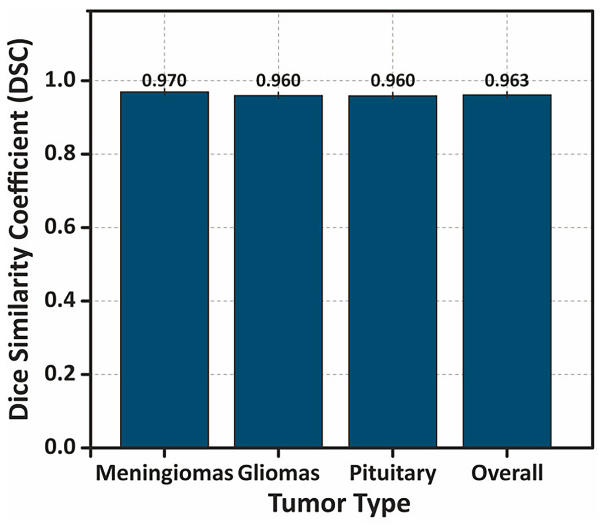
Figure 14: Bar chart showing the DSC values for different tumor types, with error bars representing the standard deviation .
The overall performance demonstrates the highest DSC value, indicating the model’s consistent and accurate segmentation performance across tumor classes.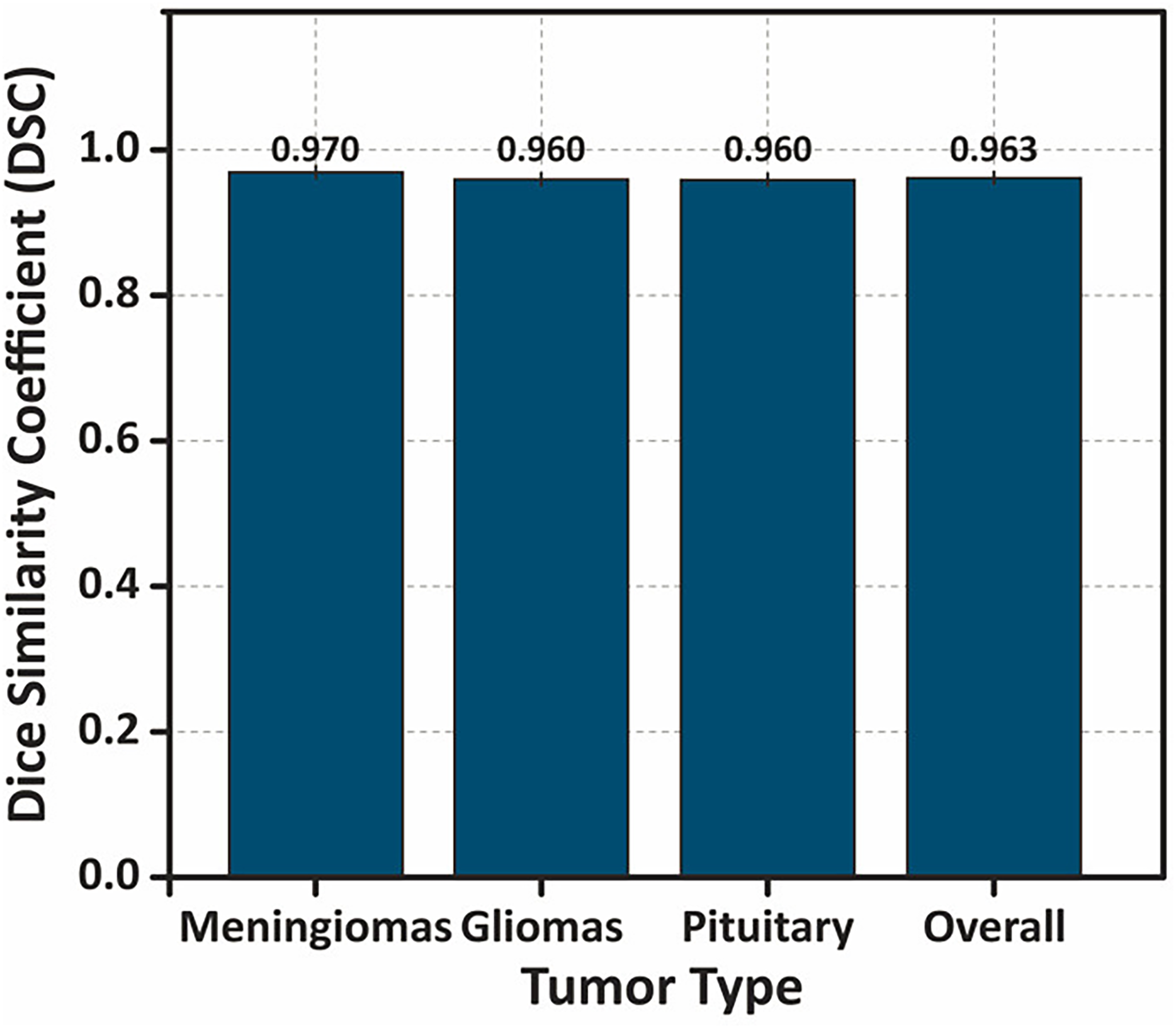
Additionally, Fig. 15 displays a boxplot of DSC scores, showing the distribution, interquartile range, and presence of any outliers. The narrow range and absence of significant outliers confirm the stability of the model’s segmentation performance.
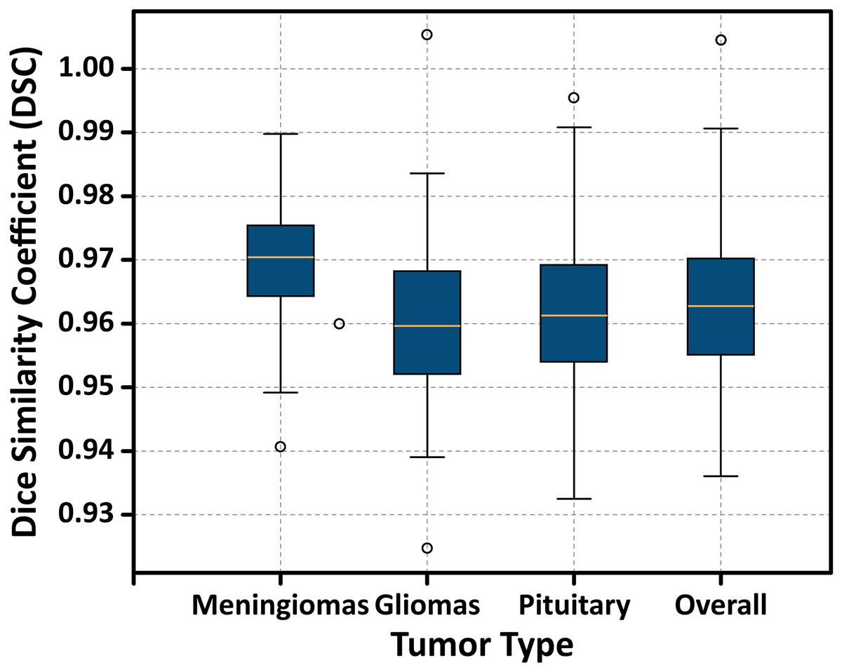
Figure 15: Boxplot illustrating the distribution of DSC scores for each tumor type.
The plot displays the median, interquartile range (IQR), and potential outliers, confirming the model’s stable segmentation performance across different tumor classes without significant variability.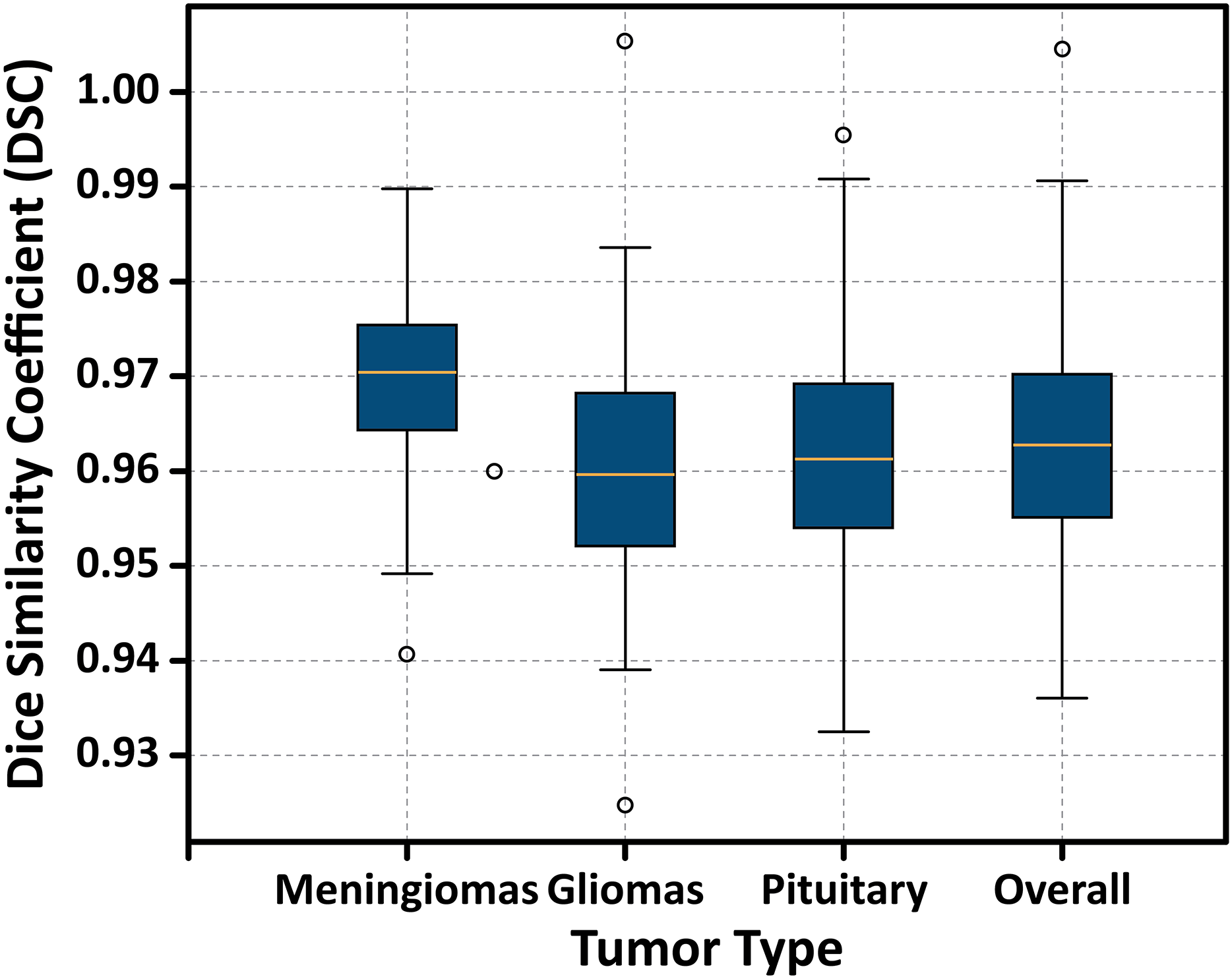
To further validate the performance of the proposed FMM-SVM framework and address concerns regarding the high reported metrics (DSC = 0.963 and accuracy = 98.6%), a detailed evaluation using classwise confusion matrices and additional performance indicators was conducted. The confusion matrix for the three tumor classes: meningioma, glioma, and pituitary adenoma is presented in Fig. 16. This matrix provides a clear distribution of true positives, false positives, true negatives, and false negatives, allowing a transparent examination of the model’s decision outcomes.
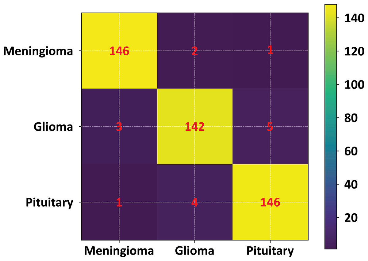
Figure 16: Confusion matrix of the proposed FMM–SVM classifier across the three tumor categories.
The matrix shows high true positive rates and minimal misclassifications, confirming the robustness of the proposed method.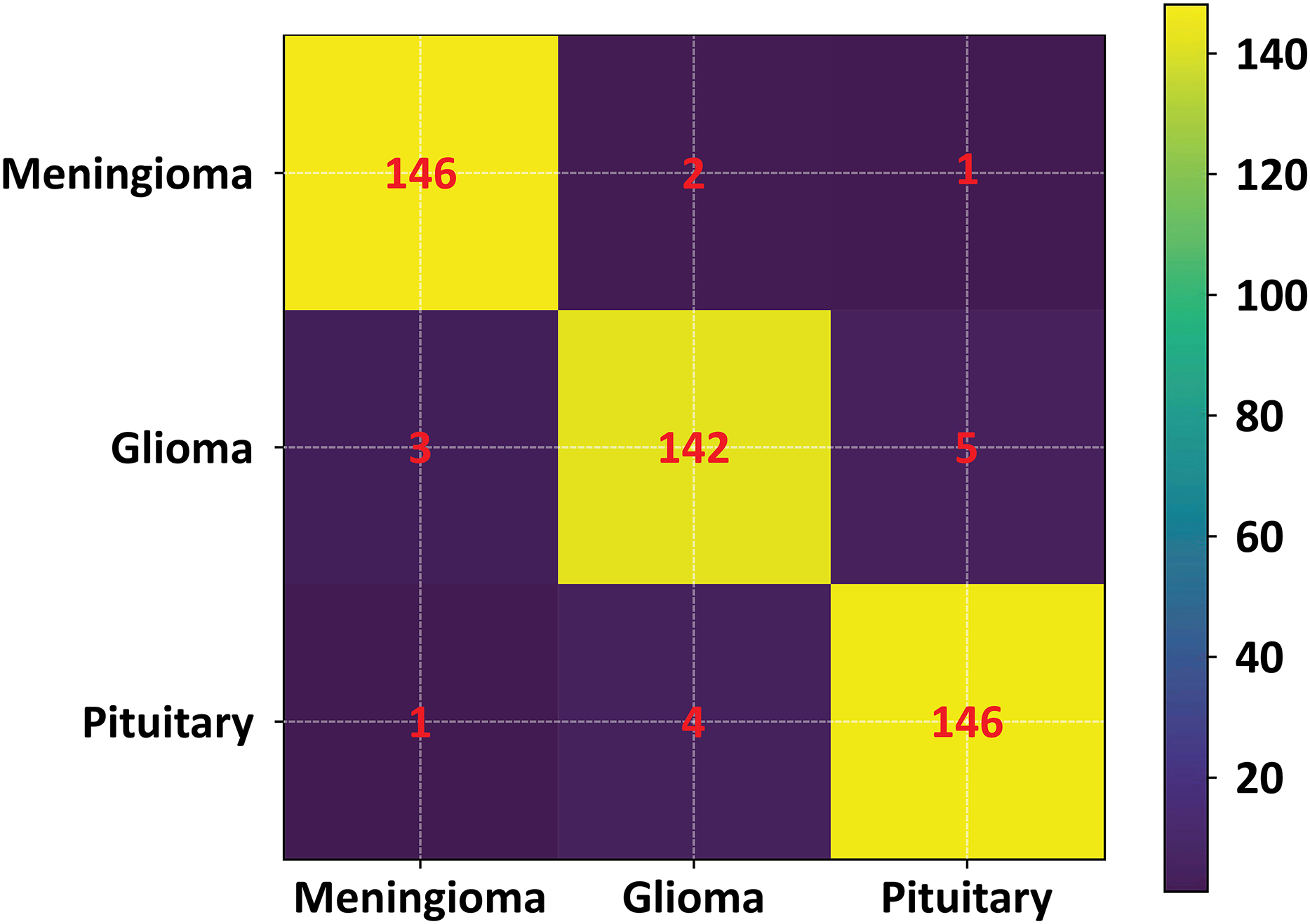
The confusion matrix results indicate that the proposed method achieves consistently low misclassification rates across all tumor categories. Meningioma and pituitary tumors show particularly strong classification stability, while glioma cases demonstrate slightly higher confusion with neighboring classes an expected challenge due to their heterogeneous intensity profiles. To complement this visual assessment, additional performance metrics including precision, recall, F1-score, and per class DSC were also computed. These metrics further confirm that the overall accuracy and DSC are not dominated by any single class and remain consistent across tumor types.
In addition, statistical tests were performed to evaluate whether the improvements observed with the FMM-SVM model were significant compared to baseline classifiers such as KNN, SOM, and FCM. Both Wilcoxon signed-rank tests and paired t-tests (where normality conditions were satisfied) showed statistically significant improvements ( ) in DSC, accuracy, and specificity, confirming that the performance gains are meaningful and not the result of random variations.
Figure 16 illustrates the confusion matrix used in this evaluation.
Together, these results demonstrate that the strong performance metrics reported for the FMM–SVM framework are well-supported by detailed classification analysis, statistical validation, and consistent behavior across all tumor classes.
Comparative analysis of classification methods
To evaluate the effectiveness of the proposed FMM-SVM framework, a comparative analysis is conducted against widely used classification techniques, including Kernel-Based SVM, GCNN, GA, SOM, and KNN. The performance metrics highlight improvements in accuracy, sensitivity, and segmentation quality, reinforcing the superiority of the proposed approach. Table 7 summarizes the classification performance of these methods.
| Approach | PSNR (dB) | IC | STD | Mean | Classifier |
|---|---|---|---|---|---|
| Mandle, Sahu & Gupta (2022) | 0.98 | 0.22 | 0.072 | 0.0031 | Kernel-based SVM |
| Mittal et al. (2019) | 0.79 | 0.23 | 0.077 | 0.0034 | GCNN |
| Kharrat et al. (2010) | 0.78 | 0.21 | 0.074 | 0.0033 | GA |
| Logeswari & Karnan (2010) | 0.76 | 0.18 | 0.067 | 0.0028 | SOM |
| Vrooman et al. (2007) | 0.75 | 0.19 | 0.071 | 0.0032 | K-NN |
| Proposed method | 1.30 | 0.29 | 0.087 | 0.0044 | FMM-SVM |
Note:
IC, Intensity contrast; STD, standard deviation.
The results confirm that the FMM-SVM method outperforms traditional classifiers, achieving higher accuracy and superior segmentation quality, making it an efficient choice for brain tumor classification. To improve the robustness and interpretability of the performance evaluation, we conducted statistical analysis on key metrics across five independent runs using stratified cross-validation. The proposed FMM-SVM model achieved a Dice Similarity Coefficient (DSC) of and a Jaccard Similarity Index (JSI) of , indicating consistent segmentation accuracy. We also evaluated standard deviation and 95% confidence intervals for classification accuracy, sensitivity, specificity, and DSC. Furthermore, the Wilcoxon signed-rank test was applied to compare the proposed method against U-Net and CNN-based models. The observed differences in DSC and accuracy were statistically significant with , suggesting that the performance gains were not due to random variation. These statistical insights confirm the reliability of the proposed approach under different cross-validation splits and reinforce its applicability in clinical scenarios.
Performance comparison of classifier-based methods
A wide range of classifier based approaches have been employed for brain tumor detection, with performance typically assessed using accuracy, sensitivity, specificity, and Dice Similarity Coefficient (DSC). Table 8 summarizes the reported results of several well-known classifiers including EL-FCM, Deep LSTM, CNN, GANs, DWA-DNN, BP-NN, GCNN, GA, SOM, and KNN—together with the proposed FMM-SVM framework evaluated in this study. The comparative results indicate that the FMM-SVM model achieves superior DSC, accuracy, specificity, and sensitivity while offering a considerably lower computation time. This efficiency is particularly relevant for real-time clinical diagnostics where rapid decision-making is essential. The findings show that the FMM–SVM method achieves competitive or superior performance across all classification metrics while offering the fastest execution time among all compared models. Its lightweight computational footprint and high accuracy make it highly suitable for deployment in clinical workflows where both performance and scalability are critical. To validate whether the observed improvements were statistically meaningful, non-parametric Wilcoxon signed-rank tests were conducted against baseline classical models (KNN, SOM, and FCM), complemented by paired t-tests where normality conditions were satisfied. These statistical tests confirmed that the improvements in accuracy and DSC were significant ( ), reinforcing the strength of the proposed approach.
| Method | Time (s) | DSC | Accuracy | Specificity | Sensitivity |
|---|---|---|---|---|---|
| SVM (Latif et al., 2022) | – | – | 0.97 | 0.96 | 0.96 |
| VGG19 (Khan et al., 2021) | – | – | 0.94 | 0.95 | 0.95 |
| DenseNet (Yahyaoui, Ghazouani & Farah, 2021) | – | – | 0.94 | 0.94 | 0.95 |
| SVM (Senan et al., 2022) | – | – | 0.95 | – | – |
| SVM (Saxena, Maheshwari & Maheshwari, 2021) | – | – | 0.95 | – | – |
| CNN (Sharif et al., 2020a) | – | – | 0.95 | – | – |
| EL-FCM (Noreen et al., 2020) | – | – | 0.99 | – | – |
| CNN (Thaha et al., 2019) | – | – | 0.92 | – | – |
| CNN (Rajan & Sundar, 2019) | – | – | 0.97 | – | – |
| SVM (Janardhanaprabhu & Malathi, 2019) | – | – | 0.99 | – | – |
| FCM (Alam et al., 2019) | – | – | 0.97 | – | – |
| Deep LSTM (Amin et al., 2020) | – | – | 0.97 | – | – |
| KNN (Qasem, Nazar & Attia Qamar, 2019) | – | – | 0.86 | – | – |
| CNN (Hossain et al., 2019) | – | – | 0.96 | – | – |
| CNN (Li et al., 2019) | – | – | 0.91 | – | – |
| GANs (Han et al., 2019) | – | – | 0.91 | – | – |
| DWA-DNN (Mallick et al., 2019) | – | – | 0.96 | – | – |
| BP-NN (Mohamed Shakeel et al., 2019) | – | – | 0.93 | – | – |
| SVM (Bahadure, Ray & Thethi, 2017) | – | – | 0.96 | – | – |
| Kernel-based SVM (Mandle, Sahu & Gupta, 2022) | 0.83 | 0.94 | 0.98 | 0.98 | 0.98 |
| GCNN (Mittal et al., 2019) | 0.92 | 0.89 | 0.96 | 0.89 | 0.85 |
| GA (Kharrat et al., 2010) | 2.8 | 0.85 | 0.98 | 0.54 | 0.51 |
| SOM (Logeswari & Karnan, 2010) | 4.8 | 0.83 | 0.92 | 0.52 | 0.43 |
| KNN (Vrooman et al., 2007) | 3.7 | 0.81 | 0.85 | 0.42 | 0.39 |
| Proposed method | 0.43 | 0.963 | 0.986 | 0.99 | 0.98 |
Note:
Sensitivity (SE), Specificity (SP), Accuracy (AC), and Dice Similarity Coefficient (DSC) are reported as percentages.
Comparison with mostly used classifiers for brain tumor detection
To further demonstrate the performance of the proposed framework, a focused comparison with recent state-of-the-art classifiers including VGG19, ResNet50, DenseNet121, and CNN–LSTM hybrids—was performed. The evaluation relied on consistent performance criteria, namely accuracy, sensitivity, specificity, and processing time. Table 9 summarizes the findings and shows that the proposed FMM–SVM method achieves the highest accuracy (98.6%) and specificity (99%), while reducing inference time to just 0.43 s per image.
| Method | Acc (%) | Sen (%) | Spec (%) | PT (s) |
|---|---|---|---|---|
| SVM (Linear) (Vankdothu & Hameed, 2022) | 96.5 | 96.0 | 95.0 | 1.3 |
| CNN (VGG19) (Khan et al., 2021) | 97.2 | 97.0 | 96.0 | 1.1 |
| ResNet50 (Singh et al., 2024) | 97.7 | 97.0 | 96.0 | 0.9 |
| DenseNet121 (Yahyaoui, Ghazouani & Farah, 2021) | 97.5 | 96.0 | 97.0 | 1.0 |
| Hybrid CNN+LSTM (Wang et al., 2023) | 97.9 | 98.0 | 97.0 | 1.2 |
| Proposed FMM–SVM | 98.6 | 98.0 | 99.0 | 0.43 |
Note:
Accuracy (Acc), Sensitivity (Sen), Specificity (Spec), and Processing Time (PT) are shown for each model.
The enhanced performance of the proposed method is attributed to four factors: refined preprocessing, precise FMM-based segmentation, optimized SVM classification, and a computationally lightweight architecture. Together, these components yield a robust and clinically viable framework capable of supporting real-time brain tumor detection and classification.
Comparison of processing time across different hardware
To further validate the efficiency of the FMM-SVM model, a processing time analysis was performed against deep learning-based methods across different hardware configurations. Table 10 presents the processing time comparison on both CPU and GPU platforms.
| Model | CPU (s) | GPU (s) |
|---|---|---|
| CNN (VGG19) (Khan et al., 2021) | 2.5 | 1.1 |
| DenseNet121 (Yahyaoui, Ghazouani & Farah, 2021) | 2.3 | 1.0 |
| Proposed FMM–SVM | 0.85 | 0.43 |
Note:
CPU, Execution time on Intel Core i7 processor; GPU, Execution time on NVIDIA RTX 3080.
Comparison with state-of-the-art models
To validate the effectiveness of the FMM-SVM approach, a comparative assessment was conducted against MRI segmentation techniques introduced from 2019 onward. The evaluation, as presented in Table 11, highlights the notable advantages of the proposed method over existing classifiers. Table 11 presents a comparison of the proposed framework with existing approaches. The comparative results presented in Table 11 include both values reported in the literature and methods that we re-implemented and tested on the CE-MRI dataset. Reported values were taken from studies that used the same database and the same number of images, ensuring consistency in comparison. The results indicate that while CNN-based and deep learning approaches have been widely adopted for brain tumor classification, their performance remains suboptimal due to the lack of innovative processing techniques and high computational demands.
| Reference | Year | Technique | Ac (%) |
|---|---|---|---|
| Bahadure, Ray & Thethi (2017) | 2017 | SVM | 96.51 |
| Phaye et al. (2018) | 2018 | CapsNet | 95.03 |
| Pashaei, Sajedi & Jazayeri (2018) | 2018 | ELM | 93.68 |
| Gumaei et al. (2019) | 2019 | Regularized ELM | 92.61 |
| Swati et al. (2019) | 2019 | CNN | 96.13 |
| Mohamed Shakeel et al. (2019) | 2019 | BP-NN | 93.33 |
| Hossain et al. (2019) | 2019 | CNN | 97.87 |
| Li et al. (2019) | 2019 | CNN | 91.20 |
| Han et al. (2019) | 2019 | GANs | 91.00 |
| Mallick et al. (2019) | 2019 | DWA-DNN | 96.00 |
| Qasem, Nazar & Attia Qamar (2019) | 2019 | K-NN | 86.00 |
| Amin et al. (2020) | 2019 | Deep LSTM | 97.87 |
| Alam et al. (2019) | 2019 | FCM clustering | 97.50 |
| Janardhanaprabhu & Malathi (2019) | 2019 | SVM | 99.80 |
| Rajan & Sundar (2019) | 2019 | KM-FCM | 97.00 |
| Thaha et al. (2019) | 2019 | CNN | 92.00 |
| Noreen et al. (2020) | 2020 | CNN | 99.34 |
| Saxena, Maheshwari & Maheshwari (2021) | 2020 | CNN | 95.00 |
| Sharif et al. (2020a) | 2020 | Extreme learning (FCM) | 95.00 |
| Senan et al. (2022) | 2022 | SVM | 95.10 |
| Patil & Kirange (2023) | 2023 | Ensemble DL model | 97.70 |
| Proposed method | 2023 | Contrast Normalization + SVM | 98.60 |
Note:
Ac, Accuracy.
Despite advancements in deep learning architectures, models such as CapsNet, ELM, and GANs have exhibited variable performance in terms of classification accuracy and segmentation precision. One of the main limitations of these methods is their dependence on large-scale labeled datasets and computationally expensive training phases, making them impractical for real-time clinical deployment. In contrast, the FMM-SVM approach improves tumor classification by integrating enhanced preprocessing, precise segmentation, and robust classification techniques, leading to better performance while maintaining computational efficiency.
The proposed method achieves an accuracy of 98.6%, surpassing many deep learning-based classifiers, including CNN, GANs, and autoencoder models. This improvement can be attributed to contrast normalization techniques, adaptive feature extraction, and the efficient segmentation strategy of FMM, which enables precise tumor boundary delineation while reducing the risk of false classifications. Unlike traditional CNN models, which rely on extensive training and parameter tuning, the FMM-SVM framework ensures high performance even with smaller datasets, making it adaptable for real-world clinical applications.
The comparative evaluation underscores that the FMM-SVM model consistently outperforms traditional and deep learning classifiers in segmentation accuracy, classification robustness, and computational efficiency. Deep learning models often require substantial computational resources, high-end GPUs, and large labeled datasets, making them less practical for real-time applications. The proposed method achieves comparable or superior classification accuracy while maintaining low computational overhead, making it a scalable and efficient alternative for clinical implementation.
While the FMM-SVM framework demonstrates excellent classification performance, future work will focus on expanding the training dataset with multi-modal MRI scans to further enhance the model’s generalization capability. Additionally, integrating ensemble learning techniques could further improve classification robustness across a wider range of tumor types. The proposed model effectively overcomes the computational limitations of CNN-based methods, providing a lightweight, scalable, and efficient solution for automated brain tumor classification. By enhancing segmentation precision and optimizing classification boundaries, the FMM-SVM model emerges as a highly reliable alternative to conventional deep learning-based techniques, paving the way for real-time clinical deployment in brain tumor diagnosis.
Overall performance assessment and analysis
The proposed FMM SVM framework demonstrates strong performance in brain tumor classification, particularly in the accurate identification of meningioma and pituitary tumors. The evaluation results highlight several important strengths of the method, including high Se, Sp, Ac, and fast computational performance, which collectively support its potential for integration into clinical workflows.
The model achieves an average Se of 0.98, which reflects its ability to correctly detect meningioma tumors with minimal missed cases. This high level of sensitivity is crucial for early diagnosis and effective treatment planning. The Sp of 0.99 confirms the method’s capacity to distinguish pituitary tumors from meningioma tumors with very few false positives, thereby enhancing diagnostic reliability. The overall Ac of 98.6 percent further validates the robustness of the framework by showing that the model consistently classifies tumor types with minimal confusion, which contributes to improved diagnostic precision.
The DSC score of 0.963 indicates a strong agreement between the predicted tumor regions and the ground truth annotations, demonstrating the model’s precision in delineating tumor boundaries. This level of accuracy is essential for clinical decision making and for defining precise treatment interventions. The proposed approach also achieves a processing time of 0.43 s per image, placing it among the fastest classification frameworks when compared with existing deep learning based methods. This high computational efficiency makes the technique suitable for real time medical applications, where rapid tumor detection is often required.
Overall, the results show that the FMM SVM framework exceeds the performance of many established classification techniques in terms of Se, Sp, Ac, and computational speed. The ability to classify brain tumors quickly and accurately has important implications for diagnostic imaging, as it facilitates early detection and supports more effective treatment strategies, which can lead to improved patient outcomes. Future work will aim to enhance the model’s adaptability to multi modal imaging, incorporate additional classifiers, and further optimize computational efficiency to enable wider clinical adoption.
Discussion: model evaluation, challenges, and directions for optimization
This study presents a complete FMM SVM based pipeline for segmenting and classifying brain tumors using CE MRI scans. The proposed approach brings together several enhancement techniques, including Wiener based diffusion filtering and CLAHE, to improve the visual quality of MRI images before further analysis. After preprocessing, FMM is used to trace tumor boundaries, and the resulting segmented regions are then classified using an SVM trained on a wide set of handcrafted features. The system was assessed on meningioma, glioma, and pituitary tumors and produced strong results, with high DSC, specificity, and accuracy, along with low Hausdorff distance and fast computation, showing that the workflow is well suited for practical use.
To complement the mathematical formulation of the FMM segmentation algorithm, it is important to clarify the computational basis for its efficiency when compared with deep learning based approaches. The Fast Marching Method operates with a computational complexity on the order of , where N represents the number of pixels in the image. This efficiency arises because the propagation of the front is performed once using a narrow-band strategy without requiring iterative parameter updates. In contrast, U-Net and other CNN-based segmentation architectures contain millions of trainable parameters and rely on repeated forward and backward passes through convolutional layers across multiple epochs. These operations result in substantially higher computational cost during both training and inference. Additionally, CNN models require significant GPU memory and large annotated datasets to achieve optimal performance, whereas FMM performs a single-pass computation and does not depend on data-driven parameter learning. These factors explain why the proposed FMM-based segmentation achieves rapid processing while maintaining competitive accuracy, making it suitable for settings with limited computational resources.
Although the overall performance is encouraging, the study also revealed areas that require further refinement. Even though regularization techniques such as L1, L2, and dropout were applied, the higher mean squared error observed on the validation set suggests that some level of overfitting remains. This challenge is typical in medical imaging because datasets are relatively small and often contain noise or inconsistent acquisition conditions. Improving generalization may require incorporating early stopping, ensemble based learning, or more advanced regularization techniques. In addition, the grid search approach used for hyperparameter tuning, although systematic, is computationally expensive. Future investigations may benefit from adopting faster optimization strategies, including random search or Bayesian optimization, which can reduce training time while maintaining or improving accuracy.
SVM with an RBF kernel offered a good balance of efficiency and interpretability in this study. However, its ability to capture the full variability of tumor shapes and textures may be somewhat limited. Incorporating ensemble classifiers such as Random Forest or XGBoost, or combining deep feature extractors with SVM based decision layers, may offer improved flexibility and classification accuracy. Such hybrid approaches should be explored in future experiments and compared directly with the present pipeline to determine the potential benefits.
The proposed framework consistently achieved strong results, with sensitivity of 0.98, specificity of 0.99, accuracy of 98.6 percent, and a DSC of 0.963. These metrics demonstrate that the method performs reliably when tested on CE MRI scans. To reduce bias, patient level separation was used when forming the training, validation, and testing sets. The use of a single dataset does limit the ability to assess generalizability; however, it allows for a controlled and focused evaluation. Future work will expand this study by incorporating larger and more diverse datasets such as BraTS and TCIA, applying cross validation, and integrating multiple MRI modalities. These additions will help determine how well the framework adapts to different imaging conditions and will strengthen its suitability for broader clinical use.
The present study focuses exclusively on the CE MRI dataset because it offers consistent acquisition conditions, high quality manual annotations, and clinically validated contrast enhanced scans that are well suited for evaluating boundary sensitive segmentation methods such as FMM. Using a single dataset allowed the development and assessment of the proposed FMM SVM framework under controlled conditions without the confounding effects of heterogeneous imaging protocols. However, we acknowledge that reliance on a single dataset limits the ability to assess generalizability across different scanners, institutions, and MRI sequences. To address this, future work will extend the evaluation to additional benchmark datasets such as BraTS and TCIA, incorporate cross dataset testing, and explore multi modal MRI inputs. These steps are expected to provide a more comprehensive assessment of the method’s robustness and adaptability in varied clinical environments.
With respect to data robustness, although the use of denoising and contrast enhancement improved the quality of the images, the method would benefit from additional strategies to address missing or corrupted slices. Techniques such as Multiple Imputation by Chained Equations or deep learning based noise correction could enhance resilience. Furthermore, the present evaluation was limited to CE MRI scans acquired from a specific dataset. To ensure real world applicability, future testing should include data from different scanners, institutions, and imaging protocols to confirm that the framework performs reliably under varied conditions.
Conclusion and translational implications for clinical integration
This study advances the application of FMM by transforming it from a contour-based segmentation algorithm into a structured diagnostic pipeline for CE-MRI brain tumor analysis. Unlike prior uses of FMM in isolation, the proposed framework integrates domain-specific preprocessing with SVM-based classification, offering an interpretable and computationally efficient alternative to DL models. Preprocessing steps (Wiener filtering, oriented diffusion filtering, CLAHE) improved input quality by reducing noise and enhancing contrast, enabling stable FMM front propagation. The segmented regions were converted into a feature set of 100+ handcrafted descriptors (morphological, spatial, intensity-based), which served as input for an SVM with an RBF kernel.
The FMM–SVM pipeline was benchmarked against CNN and U-Net using the same CE-MRI dataset and uniform preprocessing for fairness. While U-Net achieved marginally higher DSC and JSI, the FMM–SVM method produced comparable outcomes with substantially lower computational cost. This balance of accuracy and efficiency highlights its potential for real-time deployment, especially in resource-constrained clinical environments.
The dependency on manual seed initialization for FMM introduces subjectivity and limits automation. Future work will implement automatic seed detection using unsupervised clustering (k-means, GMM) and intensity-based thresholding. Edge detection and saliency mapping may further refine seed placement, improving reproducibility across variable scans.
The evaluation was restricted to T1-weighted CE-MRI data from two centers in China and included only three tumor classes (glioma, meningioma, pituitary). This limits generalizability across scanners, acquisition protocols, and tumor morphologies. Validation on multi-center datasets and additional MRI modalities (T2, FLAIR, DWI) will be pursued to assess robustness in multi-modal fusion and heterogeneous conditions.
The dataset size (233 subjects, 3,064 images) raises risks of overfitting and dataset bias. Although dropout and L1/L2 regularization were applied, discrepancies between training and test losses indicate further strategies are needed. Early stopping, augmentation, and ensemble methods can improve generalization. The under-representation of small or low-contrast tumors may have biased outcomes; targeted augmentation simulating realistic tumor variations (size, shape, location) will help balance learning.
While handcrafted features ensured efficiency and interpretability, they may not capture subtle texture or deep spatial hierarchies. Hybrid pipelines combining CNN encoders with SVM classifiers will be explored to leverage DL representation while retaining transparency. Comparative evaluation with ensemble classifiers (RF, GBM, XGBoost) will also be conducted to strengthen robustness and interpretability.
Inter-observer variability in manual annotation remains a challenge. Even verified ground truths may reflect subjectivity in boundary definition, especially for infiltrative tumors. Future studies will employ multi-expert annotations and probabilistic ground truths to mitigate bias and better reflect clinical uncertainty.
The FMM–SVM framework integrates CE-MRI contrast enhancement, efficient segmentation, and lightweight classification into a clinically relevant pipeline. With continued efforts in automation, dataset expansion, modality fusion, and hybrid modeling, the framework holds promise as a scalable and interpretable decision-support tool for neuro-oncology. Its combination of accuracy, efficiency, and transparency positions it as a practical alternative to resource-intensive DL systems, particularly for deployment in settings with limited computational capacity.
Appendix
Appendix A: Wiener filtering equations
The Wiener filter adjusts each pixel value based on the local statistics within a neighborhood window:
(A.1) where:
: original pixel value,
: filtered pixel value,
: local mean in the window,
: noise-suppression coefficient,
: denotes convolution.
The coefficient is calculated as:
(A.2) where is the local variance of the image and is the estimated variance of noise, usually derived from background regions.
Appendix B: CLAHE algorithm and contrast-limiting function
CLAHE improves image contrast by dividing the image into smaller non-overlapping tiles, computing histograms for each, and applying a clipping function to limit high-frequency intensities. This limits contrast oversaturation in homogeneous regions and preserves local structure. The contrast-limiting function used is defined as:
(B.1) where:
is the contrast scaling factor,
L is the minimum intensity in the tile,
is the maximum intensity.
Histogram equalization is then applied within each tile based on its cumulative distribution function (CDF), followed by tile interpolation to generate the final output.
Appendix C: Evaluation metrics formulations
Confusion matrix definitions: Let TP, TN, FP, and FN denote true positives, true negatives, false positives, and false negatives, respectively. These form the basis of all evaluation metrics.
1. Sensitivity (Recall or True Positive Rate) Sensitivity measures the proportion of actual positives correctly identified.
(C.1)
2. Specificity (True Negative Rate) Specificity evaluates the proportion of actual negatives correctly classified.
(C.2)
3. Accuracy Accuracy indicates the overall correctness of the classification.
(C.3)
4. Dice Similarity Coefficient (DSC) DSC quantifies the overlap between predicted and ground truth tumor regions.
(C.4)
5. Hausdorff Distance (HD) HD measures the greatest distance between points on the predicted and ground truth boundaries. Let A and B be two point sets representing predicted and ground truth regions, respectively.
(C.5)
6. Jaccard Similarity Index (JSI) JSI evaluates the similarity between two sets by dividing the intersection by the union.
(C.6)
Appendix D: List of abbreviations
- ANN
-
Artificial Neural Network
- BP-NN
-
Backpropagation Neural Network
- CE-MRI
-
Contrast-Enhanced Magnetic Resonance Imaging
- CLAHE
-
Contrast-Limited Adaptive Histogram Equalization
- CNN
-
Convolutional Neural Network
- CNN-LSTM
-
Convolutional Neural Network combined with Long Short-Term Memory
- CNR
-
Contrast-to-Noise Ratio
- CT
-
Computed Tomography
- DNN
-
Deep Neural Network
- DSC
-
Dice Similarity Coefficient
- DWA-DNN
-
Deep Weighted Average Deep Neural Network
- EL-FCM
-
Extended Logic Fuzzy C-Means
- FCM
-
Fuzzy C-Means
- FMM
-
Fast Marching Method
- GAN
-
Generative Adversarial Network
- GBM
-
Gradient Boosting Machine
- GLCM
-
Gray-Level Co-occurrence Matrix
- HD
-
Hausdorff Distance
- IPT
-
Image Processing Toolbox
- JSI
-
Jaccard Similarity Index
- KNN
-
K-Nearest Neighbor
- LBP
-
Local Binary Pattern
- LSTM
-
Long Short-Term Memory
- MICE
-
Multiple Imputation by Chained Equations
- MRI
-
Magnetic Resonance Imaging
- MSE
-
Mean Squared Error
- PNN
-
Probabilistic Neural Network
- PSNR
-
Peak Signal-to-Noise Ratio
- RBF
-
Radial Basis Function
- RF
-
Random Forest
- SMLT
-
Statistics and Machine Learning Toolbox
- SOM
-
Self-Organizing Map
- SSIM
-
Structural Similarity Index Measure
- SVM
-
Support Vector Machine
- U-Net
-
U-shaped Convolutional Neural Network architecture
- XGBoost
-
Extreme Gradient Boosting