
Multi-step-ahead forecasting of bike-sharing demand using multilayer perceptron model with additional timestamp features
- Published
- Accepted
- Received
- Academic Editor
- Ana Maguitman
- Subject Areas
- Algorithms and Analysis of Algorithms, Artificial Intelligence, Data Mining and Machine Learning, Data Science, Neural Networks
- Keywords
- Bike sharing, Artificial neural network, Forecasting, Machine learning, Timestamps
- Copyright
- © 2026 Alfian et al.
- Licence
- This is an open access article distributed under the terms of the Creative Commons Attribution License, which permits unrestricted use, distribution, reproduction and adaptation in any medium and for any purpose provided that it is properly attributed. For attribution, the original author(s), title, publication source (PeerJ Computer Science) and either DOI or URL of the article must be cited.
- Cite this article
- 2026. Multi-step-ahead forecasting of bike-sharing demand using multilayer perceptron model with additional timestamp features. PeerJ Computer Science 12:e3472 https://doi.org/10.7717/peerj-cs.3472
Abstract
Bike sharing is increasingly gaining popularity as an affordable and environmentally friendly mode of transportation in urban areas. However, the nature of bike sharing, where users can pick up and return bikes at different stations, often results in an uneven distribution of bikes across stations. Consequently, accurately predicting the future number of rented bikes at each station becomes crucial for bike-sharing operators to optimize the bike inventory at each location. This study introduces a multi-step-ahead forecasting model that employs machine learning methods to predict the hourly demand for rented bikes. We utilize information on rented bikes from the preceding day to forecast the forthcoming counts of rented bikes for the next 1, 3, 6, 12, and 24 h. Additional features extracted from timestamps are incorporated to enhance the accuracy of the model. We compare the proposed model, based on multilayer perceptron (MLP), with various machine learning prediction algorithms, including Support Vector Regression (SVR), K-Nearest Neighbor (KNN), Decision Tree (DT), Adaptive Boosting (AdaBoost), Random Forest (RF), and Linear Regression (LR). Applying the proposed MLP model to the Seoul bike-sharing dataset demonstrates a positive outcome, indicating a reduction in prediction error compared to other forecasting models. The proposed model achieves the highest R2 (coefficient of determination) values when compared to other models, with values of 0.973, 0.882, 0.82, 0.807, and 0.79 for prediction horizons of 1, 3, 6, 12, and 24 h, respectively. By obtaining future values for predicted rented bikes, the trained model is anticipated to assist in optimizing the number of available bikes for bike-sharing companies.
Introduction
Bike sharing is an innovative urban transportation system that provides a convenient and sustainable mode of travel for individuals within cities. This model allows users to rent bicycles for short-term use, typically from strategically located docking stations, and then return them at different stations across the city (DeMaio, 2009; Fishman, Washington & Haworth, 2013; Liu et al., 2019; Ploeger & Oldenziel, 2020). The primary benefit of bike sharing lies in its contribution to addressing various urban challenges. Firstly, it offers a cost-effective and eco-friendly alternative to traditional modes of transportation, promoting environmental sustainability (Bullock, Brereton & Bailey, 2017; Chen et al., 2022; Yu et al., 2018). Secondly, bike sharing facilitates the reduction of traffic congestion (Huang & Xu, 2023; Wang & Zhou, 2017) and air pollution by encouraging the use of bicycles for short-distance commutes (Huang, Zhang & Xu, 2022; Otero, Nieuwenhuijsen & Rojas-Rueda, 2018). Additionally, it enhances the overall mobility of urban residents, providing a flexible and efficient means of transportation for short trips (Cai, Ong & Meng, 2023; Caulfield et al., 2017). Moreover, bike sharing promotes a healthier lifestyle by encouraging physical activity and exercise, contributing to the well-being of individuals, and fostering a more active and vibrant urban community (Clockston & Rojas-Rueda, 2021; Nieuwenhuijsen & Rojas-Rueda, 2020).
Predicting bike-sharing demand is of paramount importance as it facilitates the efficient management and optimization of urban mobility systems (Maleki Vishkaei et al., 2020). Accurate forecasts enable service providers to anticipate user demand, strategically allocate resources, and prevent issues such as bike shortages or surpluses at specific locations (Liu & Dong, 2023; Zhang et al., 2023; Zhou et al., 2022). This proactive approach enhances the overall functionality and user satisfaction of bike-sharing systems. An effective solution lies in leveraging artificial intelligence (AI), particularly through the application of machine learning and deep learning as prediction models. Previous studies have evidenced the successful implementation of these prediction models across diverse domains, including healthcare (Allgaier et al., 2023; Coelho et al., 2023; Neto et al., 2024), inventory management (Alfian et al., 2023, 2020; Demizu, Fukazawa & Morita, 2023), smart agriculture (Dash et al., 2022; Ribeiro Junior et al., 2022; Tace et al., 2022), manufacturing (Ahmad & Rahimi, 2022; Li, Huang & Ning, 2023; Wang et al., 2024b), etc.
By harnessing sophisticated artificial intelligence, machine learning, and deep learning models, extensive datasets, including historical usage patterns, weather conditions, and temporal factors, can be analyzed to identify intricate relationships and provide accurate predictions. This data-driven AI approach, utilizing machine learning and deep learning models for bike-sharing demand prediction, is pivotal in enhancing the overall quality of bike-sharing services. Past studies have demonstrated the application of prediction models to estimate the current usage of rented bikes (Boonjubut & Hasegawa, 2022; Gao & Chen, 2022; Harikrishnakumar & Nannapaneni, 2023; Li et al., 2023; Lv et al., 2021; Mehdizadeh Dastjerdi & Morency, 2022; Peláez-Rodríguez et al., 2024; Sathishkumar, Park & Cho, 2020a, 2020b; Sathishkumar & Cho, 2020a, 2020b; Xu, Ji & Liu, 2018; Xu et al., 2020; Yang et al., 2020). Furthermore, researchers have incorporated multi-step forecasting models not only to gauge the existing demand for rented bikes but also to anticipate their future utilization, providing valuable insights into the evolving patterns of bike-sharing systems (Gammelli et al., 2022; Gao & Lee, 2019; Hua et al., 2020; Leem et al., 2023; Luo et al., 2021; Ma et al., 2022; Zhou et al., 2021). These forecasting techniques contribute significantly to operational efficiency, aiding in the proactive management and strategic planning of bike-sharing services. Additionally, they play a pivotal role in enhancing user experience and overall system sustainability.
The focus of past studies has predominantly been on estimating the current usage of rented bikes, with a limited emphasis on multi-step-ahead forecasting. This gap in research highlights the need for improvement in predicting the future demand for bike-sharing, which is crucial for ensuring the efficient management of bike-sharing services. Previous studies have shown significant improvements in bike-sharing demand prediction by incorporating machine learning approaches. However, there remains a need for comparative analysis with other machine learning models to determine the most effective multi-step ahead forecasting methods. Therefore, this study introduces a novel multi-step-ahead forecasting technique utilizing a multilayer perceptron (MLP) to predict future bike-sharing demand, aiming to evaluate its performance against alternative machine learning approaches. Additionally, the incorporation of timestamp features is anticipated to enhance the accuracy of the multi-step-ahead forecasting model.
Literature review
In recent years, extensive research has been conducted in bike-sharing systems, with a particular focus on enhancing operational efficiency through the prediction of bike-sharing demand. Researchers have explored various forecasting models, leveraging diverse datasets and advanced methodologies for bike-sharing demand prediction in urban environments. The research in the bike-sharing demand prediction can be categorized into two distinct yet interconnected domains: one focusing on predicting the current bike-sharing demand to facilitate real-time operational decisions, and the other delving into forecasting future demand patterns (multi-step-ahead forecasting) to enhance strategic planning and system optimization.
Numerous studies have explored the prediction of current bike-sharing demand, examining various methodologies and approaches to enhance the real-time understanding of user needs and operational dynamics in the context of bike-sharing systems. Previous study focuses on developing a dynamic demand forecasting model for station-free bike sharing in China using long short-term memory neural networks (LSTM NNs). The developed LSTM NNs demonstrate superior prediction accuracy compared to conventional statistical models and advanced machine learning methods, offering valuable insights for rebalancing sharing bikes within the system (Xu, Ji & Liu, 2018). Xu et al. (2020) proposed a hybrid edge-computing-based machine learning model, combining a self-organizing mapping network with a regression tree. The proposed method demonstrated higher accuracy in predicting number of bikes compared to previous approaches, as evidenced by experiments using real data from the Washington and London bike-sharing systems. Lv et al. (2021) proposed three-layer ensemble learning model (SAP-SF) integrates features such as subway station-related site categories, bike-sharing site mobility patterns, and various environmental factors, outperforming benchmark models and providing valuable insights for system administrators to enhance service levels and rebalance bike-sharing systems around subway stations. Boonjubut & Hasegawa (2022) evaluated forecasting algorithms using historical, weather, and holiday data from three databases. The study proposed various artificial intelligence techniques to accurately predict bike-sharing demand, providing valuable insights for operators to plan and manage the rebalancing process effectively.
The prediction of current bike-sharing demand in the context of Seoul City has been a subject of considerable research, with studies delving into diverse methodologies to improve the accuracy and efficiency of forecasting models in addressing the unique challenges of the city’s bike-sharing system. Sathishkumar, Park & Cho (2020a) focuses on predicting hourly rental bike demand in urban cities to ensure a stable supply, employing a data mining technique that considers weather information, date details, and the number of bikes rented. Five statistical regression models, including Linear Regression and Gradient Boosting Machine, were trained and evaluated, with the latter achieving the highest values of 0.96 in the training set and 0.92 in the test set when using all predictors. Furthermore, another study revealed that Temperature and Hour of the day as the most influential variables in hourly rental bike demand prediction (Sathishkumar & Cho, 2020a). Sathishkumar, Park & Cho (2020b) demonstrated the effectiveness of Random Forest for accurately predicting trip duration in the context of bike-sharing systems. The result achieves an impressive 93% variance explanation in the testing set and 98% ( ) in the training set. Finally, previous study reveals the influence of different characteristics varies with seasons, suggesting the need to consider seasonal changes for improved bike sharing demand predictions, as demonstrated by Random Forest (RF) models trained on both yearly and season-wise data (Sathishkumar & Cho, 2020b).
Furthermore, many research endeavors have been dedicated to predicting the current bike-sharing demand through the application of both machine learning and deep learning techniques, reflecting a concerted effort to employ advanced methodologies for real-time insights into the dynamics of bike-sharing systems. Peláez-Rodríguez et al. (2024) evaluate the performance of various Machine Learning and Deep Learning approaches for forecasting bike-sharing demand in Madrid and Barcelona, Spain, as well as cable car demand in Madrid. Gao & Chen (2022) utilized four machine learning models—linear regression, k-nearest neighbors, random forest, and support vector machine. The random forest model stands out as the most effective performer, achieving an of 0.93, with weather, pollution, and COVID-19 outbreak features recognized as the key predictors for precise demand forecasting. Another study reported the bike demand in Montreal and demonstrated that deep learning models, particularly the hybrid Convolutional Neural Network-Long Short Term Memory (CNN-LSTM), outperform the benchmark ARIMA model, with additional variables improving overall prediction accuracy and providing valuable insights for bike-sharing operational management (Mehdizadeh Dastjerdi & Morency, 2022). Li et al. (2023) demonstrated irregular convolutional Long-Short Term Memory model (IrConv+LSTM) outperforms benchmark models in various cities and during peak periods, emphasizing the importance of considering spatial variations in built environment characteristics and travel behavior for improved short-term demand prediction in urban bike-sharing systems. Yang et al. (2020) focused on enhancing short-term demand prediction in bike-sharing schemes by incorporating novel time-lagged graph-based variables extracted from real-world bike usage datasets. Results demonstrated that these graph attributes are more influential in demand prediction than traditional meteorological information, with LSTM proving particularly effective in handling the sequences of time-lagged graph variables for more accurate forecasting in urban areas. Finally, Harikrishnakumar & Nannapaneni (2023) emphasize the role of quantum computing algorithms for computational speedup compared to classical algorithms. The study illustrates the construction of Quantum Bayesian Networks (QBN) and provides a solution framework for two case studies, comparing the performance of quantum and classical solutions using IBM-Qiskit and Netica computing platforms.
Another approach used to forecast the future number of rented bikes in bike sharing is known as multi-step-ahead forecasting. Multi-step-ahead forecasting is crucial in the context of bike-sharing demand as it enables system operators and planners to anticipate future demand patterns over an extended time horizon. By predicting demand not just for the immediate future but for several steps ahead, bike-sharing systems can better adapt to changing conditions and optimize their operations. This is particularly important in urban environments where demand fluctuates throughout the day, week, or even seasonally. Numerous research studies have focused on multi-step-ahead forecasting for bike-sharing demand, employing various methodologies to anticipate usage patterns and trends. Gao & Lee (2019) proposed a moment-based model and a hybrid approach that combines a fuzzy C-means (FCM)-based genetic algorithm (GA) with a backpropagation network (BPN). The FCM-based GA pre-classifies historical rental records, and the results are utilized by a BPN predictor to forecast demand at future moments, demonstrating effectiveness and efficiency in a real-life case study. Gammelli et al. (2022) introduced a variational Poisson recurrent neural network model (VP-RNN) for forecasting future pickup and return rates. Leem et al. (2023) proposed an online learning-based two-stage forecasting model designed for low-computing environments with insufficient data, aiming for robust and fast multi-step-ahead prediction of bike-sharing demand in Seoul. The model, applied to the Seoul Bike-sharing Demand dataset, utilizes random forest, extreme gradient boosting, and Cubist methods in the first stage, followed by the Ranger package trained with external factors in the second stage, demonstrating superiority over 23 other machine and deep learning models.
Previous methods utilizing machine learning and deep learning techniques for multi-step-ahead forecasting in bike sharing demand have been introduced and demonstrated notable outcomes. Ma et al. (2022) introduced a Spatial-Temporal Graph Attentional Long Short-Term Memory (STGA-LSTM) neural network framework for predicting short-term bike-sharing demand at a station level, utilizing multi-source datasets including historical bike-sharing trip data, weather data, user information, and land-use data. Hua et al. (2020) employed RF for real-time predictions of passenger departure, arrival, and bike count in these stations. The results show a positive correlation between bike count and usage, with RF providing accurate predictions that outperform benchmark methods, offering insights for dockless bike-sharing (DBS) companies to dynamically rebalance bikes from oversupply to demand regions more effectively. Zhou et al. (2021) introduced a deep neural network model, ST-HAttn, with spatiotemporal hierarchical attention mechanisms for Multi-step Station-Level Crowd Flow Prediction (Ms-SLCFP). The model employs attention mechanisms at both station and regional levels, explicitly modeling pairwise correlations of station-region to address challenges posed by complicated spatiotemporal correlations and fluctuations in crowd flow, demonstrating superior performance over state-of-the-art methods on real-world datasets. Luo et al. (2021) presented the LSGC-LSTM model, a novel approach for predicting pickup and return demands in docked bike-sharing systems using multi-source data. This method integrates Local Spectral Graph Convolution (LSGC) and LSTM networks to capture both spatial and temporal dependencies in bike-sharing demand. The LSGC-LSTM model outperforms six baseline models in terms of prediction accuracy and efficiency. Finally, Zhou et al. (2019) proposed an encoder-decoder neural network that integrates convolutional layers with LSTM units to capture spatial and temporal dynamics. To enhance multi-step forecasting, they incorporated a multi-level attention mechanism—global and temporal—to account for representative demand patterns and dynamic correlations over time. Experimental results demonstrated that the proposed method outperformed baseline models across most evaluation metrics on two real-world datasets. The summarized studies are outlined in Table 1. Upon analyzing these various approaches, it becomes evident that they collectively concentrate on forecasting the current and future demand for bicycles, taking into account factors such as weather conditions, time, and seasons. Predicting current conditions alone has limitations because it does not provide insights into what may happen in the future. Multi-step-ahead forecasting allows us to estimate future trends, potential challenges, and opportunities, enabling better preparation, resource allocation, and decision-making. Consequently, the development of a dedicated multi-step-ahead forecasting model becomes imperative for predicting the future demand for bike sharing. In line with this, we introduce a novel contribution by proposing a multilayer perceptron model integrated with timestamp features to enhance the accuracy of multi-step-ahead forecasting bike demand.
| Authors | Purpose | Input features | Method | Dataset | Result |
|---|---|---|---|---|---|
| Xu, Ji & Liu (2018) | Predicting bike sharing trip | Trip, weather, air quality, land use | LSTM | Nanjing city | MAPE up to 12.542 |
| Xu et al. (2020) | Predicting bike sharing demand | Weather, date time information, and the number of bikes rented | Self-organizing mapping network with a regression tree (SOM-RT) | Washington shared bike dataset | MAE = 14.651, RMSE = 6.564 |
| Lv et al. (2021) | Predicting bike sharing demand | Weather, Air quality, POI, Subway station related site category, Site mobility pattern, Bike trip | SAP-SF | Beijing | RMSE = 10.9171, = 0.6882 |
| Boonjubut & Hasegawa (2022) | Predicting current rented bike | Weather, date time information, and the number of bikes rented, seasonality | Gated recurrent units (GRU) | Citi bike in Jersey city | = 0.82, RMSE = 15.44, MAE = 13.45 |
| Sathishkumar, Park & Cho (2020a) | Predicting current rented bike | Weather, date time information, and the number of bikes rented | Gradient boosting machine | Seoul bike 2018 | = 0.92, RMSE = 172.73, MAE = 109.78 |
| Sathishkumar & Cho (2020a) | Predicting current rented bike | Weather, date time information, and the number of bikes rented | CUBIST | Seoul bike 2018 and capital bikeshare | Seoul bike dataset. = 0.95, RMSE = 139.64, MAE = 78.45, |
| Capital bikeshare dataset. = 0.89, RMSE = 58.83, MAE = 38.47 | |||||
| Sathishkumar, Park & Cho (2020b) | Predicting current rented bike | Reservation data, weather | Random Forest | Seoul bike 2018 | RMSE = 6.25, = 0.93, MAE = 2.92 |
| Sathishkumar & Cho (2020b) | Predicting current rented bike | Weather, date time information, and the number of bikes rented, seasonality | Random Forest | Seoul bike 2018 | = 0.97, RMSE = 91.85, MAE = 60.03 |
| Peláez-Rodríguez et al. (2024) | Predicting bike sharing demand | Weather, date time information, and rental demand | Machine learning and deep learning | Spain | Up to = 0.85, RMSE = 1,441, MAPE = 25.04, MAE = 1,037.89 |
| Gao & Chen (2022) | Predicting bike sharing demand | Weather, air pollution, traffic accidents, Covid-19 outbreak, social and economic factors, and seasonality | Random forest | Seoul bike sharing | RMSE = 399.21, MAE = 264.40 |
| Mehdizadeh Dastjerdi & Morency (2022) | Predicting bike sharing demand | Trip, date time information, weather | LSTM | Montreal BIXI bike-sharing system | Up to MAE = 3.08, RMSE = 4.74 |
| (Li et al., 2023) | Predicting bike sharing demand | Bike trip records | Irregular convolutional Long-Short Term Memory model (IrConv + LSTM) | Singapore, Chicago, Washington, New York, London | London dataset. MAPE = 0.5523, MAE = 3.5785, RMSE = 6.2960 |
| Yang et al. (2020) | Predicting bike sharing demand | Weather, date time information, graph feature, and rental demand | LSTM | New York, Chicago | New York dataset. RMSE = 8.114, MAPE = 26.2 Chicago dataset. RMSE = 5.268, MAPE = 27.9 |
| Harikrishnakumar & Nannapaneni (2023) | Predicting bike sharing demand | Bike trip transaction | Quantum Bayesian Network | New York City | Up to RMSPE = 0.7 |
| Gao & Lee (2019) | Multistep ahead prediction for bike sharing demand in the next 2-h later | Weather, date time information, and rental demand | Back propagation network (BPN) |
Washington D.C., USA | RMSE 33.7, MAE 15.5 |
| Gammelli et al. (2022) | Multistep ahead prediction for station-level pickups and returns demand in the next 1-day later | Weather, date time information, and the number of bikes rented | MOVP-RNN | New York Citi bike | Pickup demand. RMSE = 3.04, MAE = 2.09, = 0.92 |
| Return demand. RMSE = 4.94, MAE = 3.43, = 0.79 | |||||
| Leem et al. (2023) | Multistep-ahead prediction for bike sharing demand in the next 1 h to 1 day later | Weather, date time information, and the number of bikes rented | Ensemble learning, Random Forest | Seoul bike 2018 | RMSE = 310.85, MAE = 213.32 |
| Ma et al. (2022) | Multistep ahead prediction for bike sharing demand in the next 15-min, 30-min, 45-min, and 60-min later | Historical bike-sharing trip, weather, users’ personal information, and land-use data | STGA-LSTM | Nanjing public bicycle company | PH 60 min for rental demand. RMSE = 0.8979, MAE = 0.5418 |
| PH 60 min for return demand. RMSE = 0.8998, MAE = 0.5440 | |||||
| Hua et al. (2020) | Multistep ahead prediction for bike sharing demand in the next 15-min, 30-min, 45-min, and 60-min later | Reservation/journey data | Random Forest | Mobike in Nanjing | PH 60 min for departure forecasting. |
| MAE = 1.758, RMSE = 3.358 | |||||
| Zhou et al. (2021) | Multistep ahead prediction for bike sharing demand up to 6-step output | Trip data | ST-HAttn | MTASubway, CitiBike, NYCTaxi | MTASubway dataset. RMSE = 495.6 |
| CitiBike dataset. RMSE = 1.878 | |||||
| NYCTaxi dataset. RMSE = 9.637 | |||||
| Luo et al. (2021) | Multistep ahead prediction for the pickup/return demands in the next 5-min, 10-min, 15-min, 20 min |
Trip data | LSGC-LSTM | Zhejiang in China | Pickup demand. For PH 20 min. RMSE = 0.786, MAE = 0.467 |
| Return demand. For PH 20 min. RMSE = 0.779, MAE = 0.460 | |||||
| Zhou et al. (2019) | Multistep ahead prediction for citywide passenger demands | Taxi and bike trips | Multi-level attention based encoder-decoder framework (MultiAttConvLSTM) | New York city | The proposed method outperformed others in terms of RMSE, MAE, and MAPE across both datasets, except for the MAPE score on the Taxi dataset. |
Note:
RMSE, Root Mean Squared Error; MAE, Mean Absolute Error; , Coefficient of Determination; MAPE, Mean Absolute Percentage Error; RMSPE, Root Mean Square Percentage Error; Multistep ahead prediction, forecasting multiple future points in a time series beyond the next one; PH, Prediction Horizon.
We chose a MLP because it has consistently delivered strong results in regression and forecasting when enriched with carefully engineered temporal inputs. While recurrent architectures like LSTM and gated recurrent unit (GRU) are designed to capture sequence dependencies, they often require much larger datasets and extensive hyperparameter tuning to outperform simpler feed-forward networks in practice (Lazcano, Jaramillo-Morán & Sandubete, 2024; Wang et al., 2024a). We anticipate that by directly encoding time-related features into our MLP, it will effectively capture temporal patterns without relying on recurrent connections. Furthermore, we expect MLPs to deliver faster training, reduced computational demands, and enhanced transparency compared to recurrent neural network (RNN)-based models, making them ideal for deployment in resource-constrained environments.
Materials and Methods
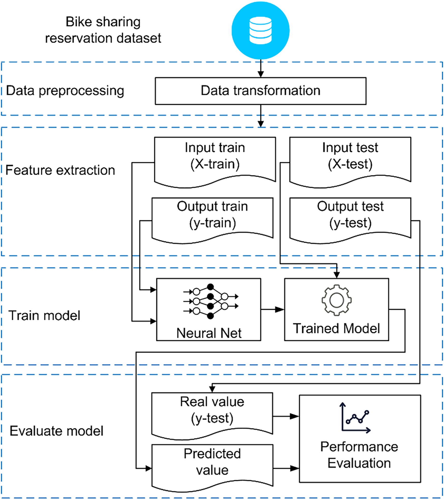
The model depicted in Fig. 1 utilizes data related to bike-sharing demand, including factors such as start-end times, departure-destination stations, and rental durations. After collecting the data, we applied a preprocessing step to remove inconsistent entries and handle missing values using mean or median imputation, depending on the data distribution. These methods were chosen because they are effective at preserving the overall structure of the data without adding complexity. Median imputation is suitable for skewed data or outliers, while mean imputation fits normally distributed data. Since the amount of missing data in our dataset was small, these simple methods were considered appropriate. As noted by Acuña & Rodriguez (2004) the difference in performance between mean and median imputation is generally minimal, especially when the effects of outliers balance out. The feature extraction technique is employed to transform time series data into an input matrix X and an output vector y. The neural network model utilizes the training data to discern patterns from a set of paired inputs and corresponding desired outputs. After the learning process is concluded, the trained model is employed to forecast the future number of rented bikes, which is then compared with actual values (ground truth) to assess the model’s performance. For model evaluation, a hold-out method is utilized, allocating the first 75% of the dataset for training and the remaining portion for testing.
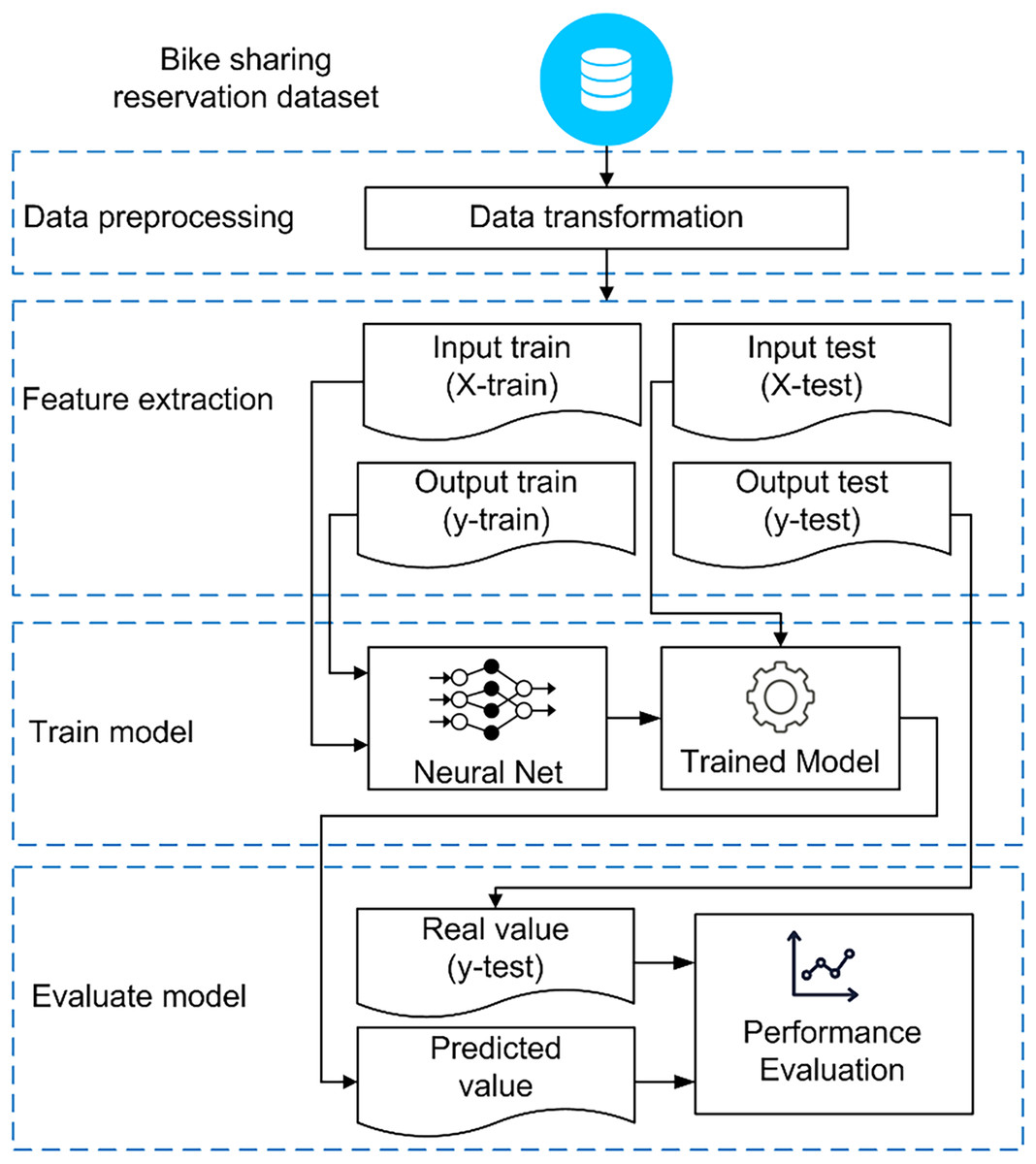
Figure 1: An overall framework for developing and assessing forecasting models.
Data preparation
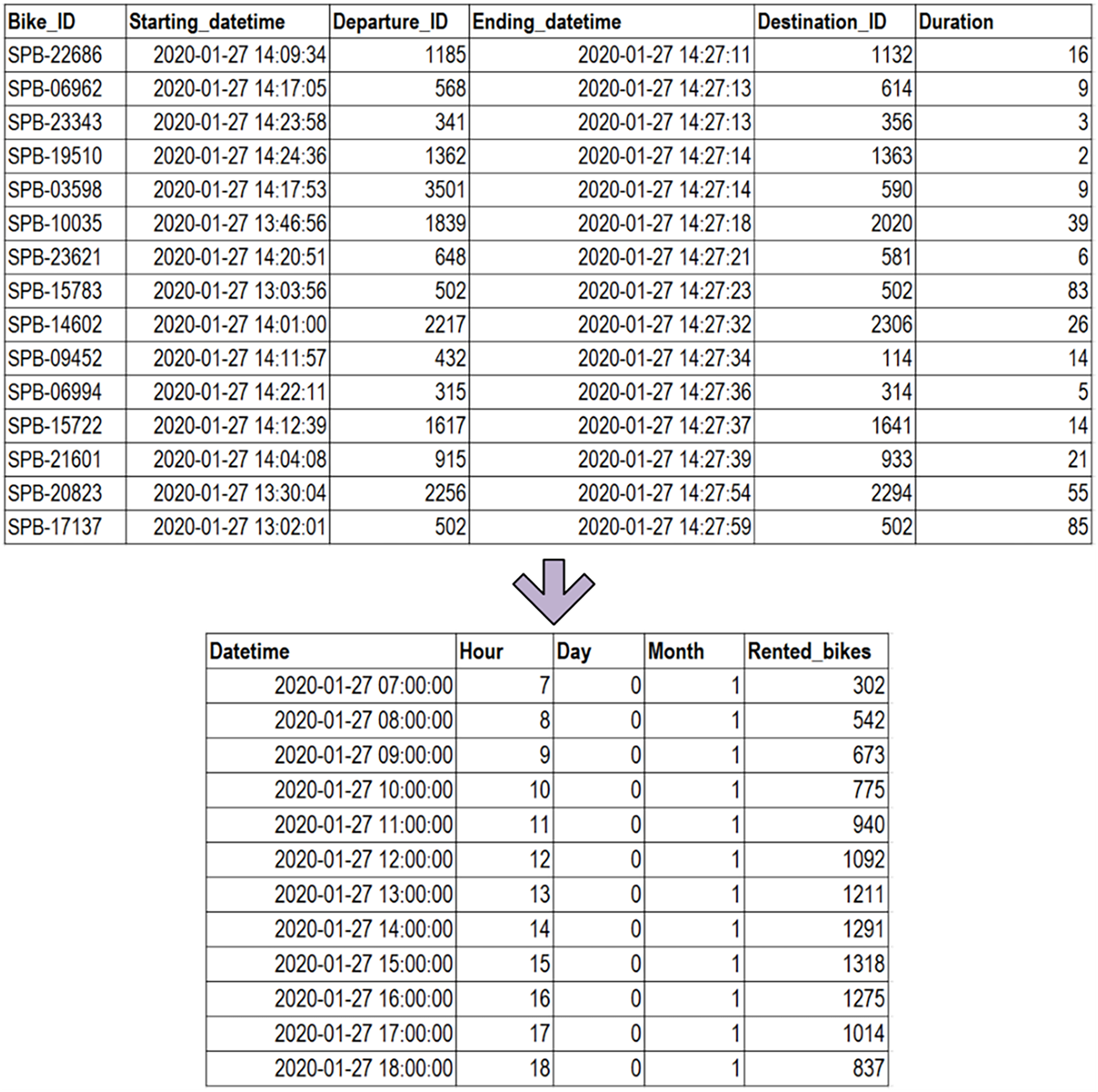
To assess the effectiveness of the prediction models, we gathered data on bike-sharing reservations in Korea. This reservation data spans from January 2020 to December 2020, encompassing a one-year period, and was obtained from Seoul Public Data (Seoul Bike Sharing, 2020). The original reservation data, as illustrated in Fig. 2, contains various columns including bike ID, starting datetime, departure ID, ending datetime, destination ID, and duration (in minutes). To construct the dataset for hourly bike demand, the reservation data needed to be reformatted, counting the total number of rented bikes for each hour. Subsequently, timestamp information was utilized to extract details such as the hour, day, and month. The resulting dataset for this study includes information on the hour, day, month, and the number of rented bikes. Table 2 provides a breakdown of the dataset description in this research.
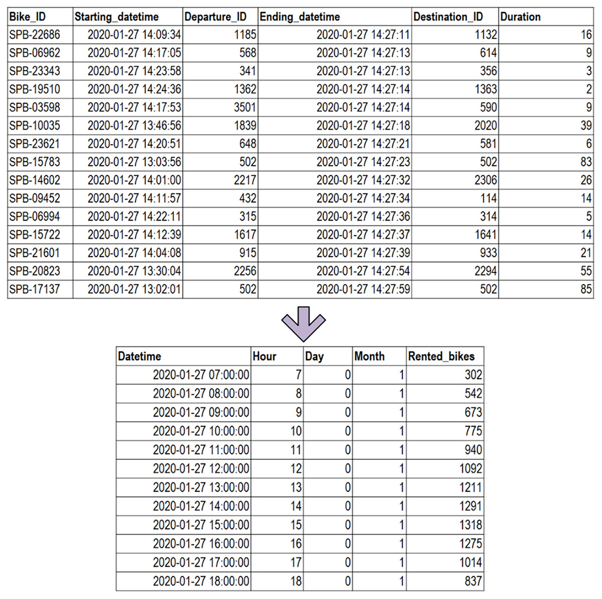
Figure 2: Transformation from reservation data to the ultimate dataset.
| No | Attribute | Type | Range | Description |
|---|---|---|---|---|
| 1 | Hour | Numeric | 0, 1, 2, …, 23 | The extracted hour is derived from the starting date. |
| 2 | Day | Numeric | 0, 1, 2, …, 6 | The extracted day corresponds to the reservation date, following a numerical representation where 0 represents Monday, 1 represents Tuesday, and so forth, with 6 representing Sunday. |
| 3 | Month | Numeric | 1, 2, 3, …, 12 | The extracted month corresponds to the starting date and is represented numerically, where 1 denotes January, and 12 represents December. |
| 4 | Rented_bikes | Numeric | 0, 1, 2, …, 10,286 | The total count of rented bikes. |
The next step is Exploratory Data Analysis (EDA), a crucial phase aimed at gaining insights into the characteristics and patterns present in the bike-sharing demand dataset. EDA involves a comprehensive examination of the data through statistical summaries, visualizations, and graphical representations. This process helps uncover trends, distributions, and patterns within the dataset. Identifying such patterns is instrumental in informing subsequent steps of the modeling process, guiding feature selection, and enhancing the overall interpretability of the model.
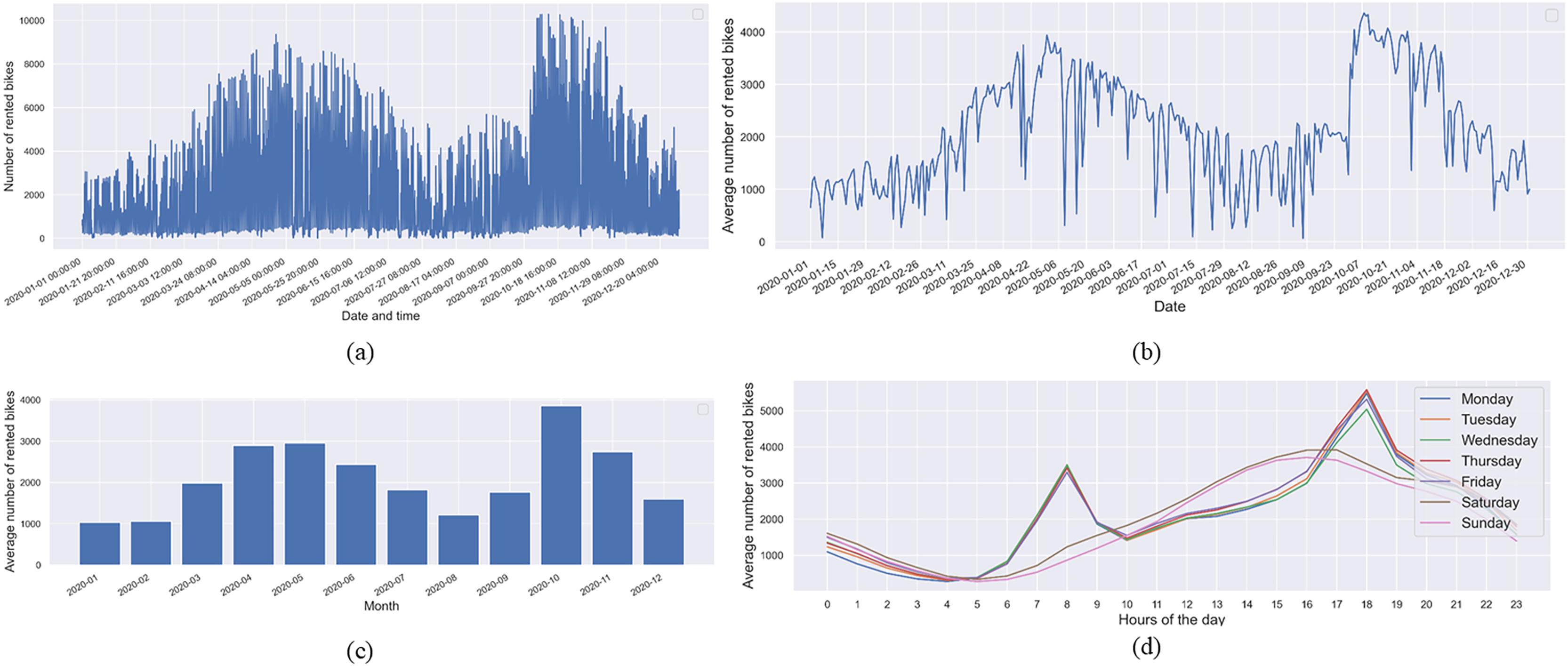
Figure 3 illustrates the count of rented bikes, depicting the average count across days, months, and hours throughout the week. The visualizations reveal a discernible temporal pattern in the rented bike numbers, highlighting the significance of these temporal dependencies for more accurate rented bike predictions. Specifically, Fig. 3A showcases the overall rented bike count, while Fig. 3B presents the daily average, revealing notable variability in bike counts at different hours and days. Figure 3C underscores that the average number of rented bikes is considerably lower during the winter months (January, February, and December) in South Korea. Conversely, peak bike rentals occur during the spring months (April, May, and June) and fall months (October and November). Furthermore, Fig. 3D displays the average rented bikes categorized by day of the week. It is evident from Fig. 3D that the average trip duration on weekdays peaks during the morning hours (7 to 9 AM) and evening hours (5 to 7 PM). On weekends, a different trend emerges, with the majority of rented bikes starting in the afternoon, specifically between 1 and 8 PM. This temporal analysis provides valuable insights into the dynamics of bike-sharing demand, laying the foundation for a more nuanced understanding of how time-related factors influence bike rental patterns. These findings are essential for refining predictive models and optimizing resource allocation in bike-sharing systems.
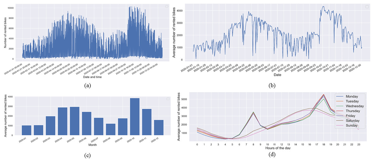
Figure 3: (A) The hourly count of rented bikes, (B) the average rented bikes by date, (C) the average rented bikes by month, and (D) the average rented bikes by hour of the day throughout weekdays.
The temporal analysis depicted in Fig. 3 not only uncovers seasonal variations in bike rental patterns but also offers implications for operational considerations in bike-sharing systems. The observed peaks in bike rentals during specific hours and seasons suggest a need for dynamic resource management. For instance, during high-demand periods such as the morning and evening rush hours on weekdays, bike-sharing systems may benefit from strategically redistributing bikes to meet increased demand in specific locations. Moreover, demand notably rises during the spring and summer months, reflecting more favorable weather and increased recreational usage. Furthermore, the comprehensive exploration of temporal dependencies in bike-sharing demand, as illustrated in Fig. 3, not only aids in predicting rented bike counts more accurately but also provides actionable insights for the strategic management and optimization of bike-sharing systems. The integration of these findings into operational practices can enhance user experiences, increase system efficiency, and contribute to the sustainable growth of bike-sharing initiatives.
Feature extraction
In the feature extraction phase, the time series dataset undergoes transformation into a collection of paired inputs (X) and corresponding desired outputs (y). The prediction process utilizes the “direct method,” which involves independently forecasting each horizon without reliance on other predictions (Ben Taieb et al., 2012; Bontempi, Ben Taieb & Le Borgne, 2013). The direct strategy autonomously learns each horizon (denoted as ) and models the corresponding function, denoted as
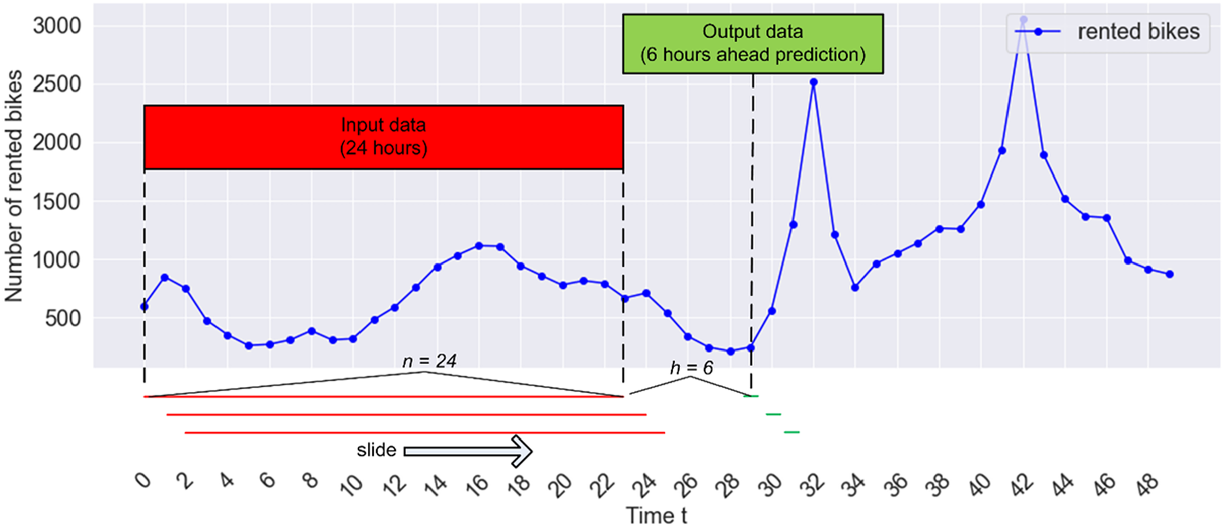
(1) with and and provides a multi-step prediction by combining the forecasts for each horizon ( ). To implement this direct strategy, the sliding window approach can be employed to segment the time series dataset, as illustrated in Fig. 4. In this scenario, input data is generated by assembling windows with a size of n = 24 for learning, aiming to predict the count of rented bikes for the subsequent h = 6. Given that the count of rented bikes was recorded every hour in our study, this prediction model utilizes the last 24 h of historical data (as features) to forecast the count of rented bikes for the next 6 h. In Fig. 4, the windows (indicated by red lines) are gathered and presented as an input matrix X, while the following 6 h of values (depicted by green lines) serve as an output vector y. The pairs of inputs and outputs are derived by shifting the window one-time step ahead on each iteration. Two parameters need consideration in this context: the window size, n, and the prediction step ahead, h. Subsequently, the collection of paired inputs and desired outputs is divided into a training set and a testing set.
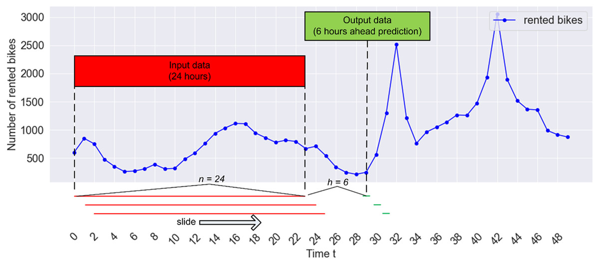
Figure 4: The sliding window technique for predicting hourly bike sharing demand.
By adhering to this process, a series of paired inputs and corresponding desired outputs can be generated, allowing the supervised learning model to glean insights from these input-output pairs. Here, C denotes the collection of rented bike counts, and signifies a specific count of rented bikes within the set, where C and i = 1, 2…, N. The parameter N represents the total number of data entries. Ultimately, with the given previous values (or window size) and the forecasting horizon, , the input matrix can be formulated by constructing a matrix of input data
(2) and the output vector
(3)
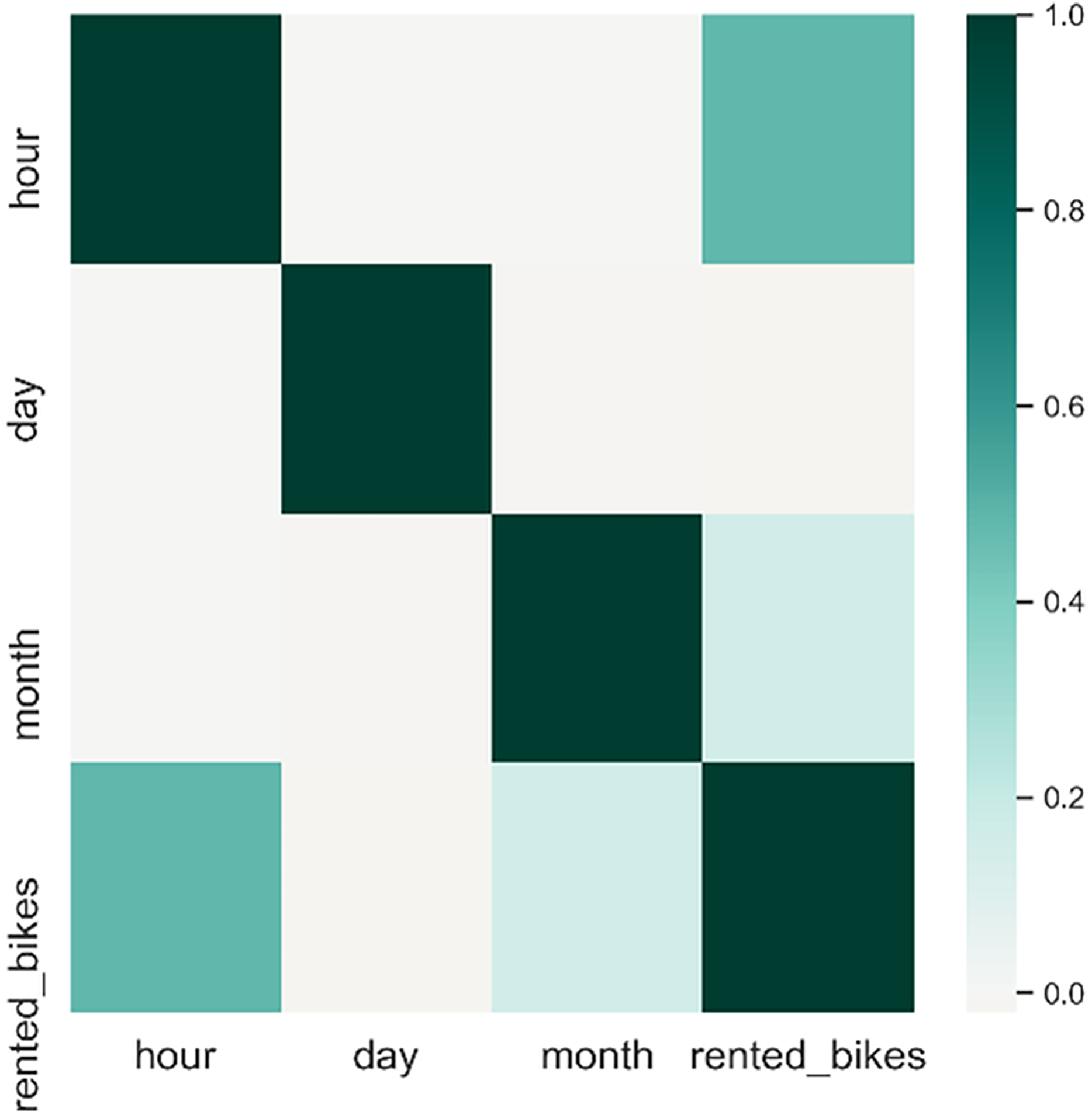
Figure 3 indicates a notable correlation between timestamps information and the count of rented bikes. Additionally, we assess the relationship between timestamp attributes and the count of rented bikes. To investigate this association, we utilized Pearson’s correlation coefficient, which ranges from −1 to +1. A negative or positive value denotes a negative or positive correlation, and a higher absolute value signifies a more robust correlation. Attributes demonstrating a substantial correlation with the output class can be utilized as input features to improve the accuracy of the prediction model. Figure 5 demonstrates that the hour of the day, day of the week, and month of the year exhibit a positive correlation with the output.
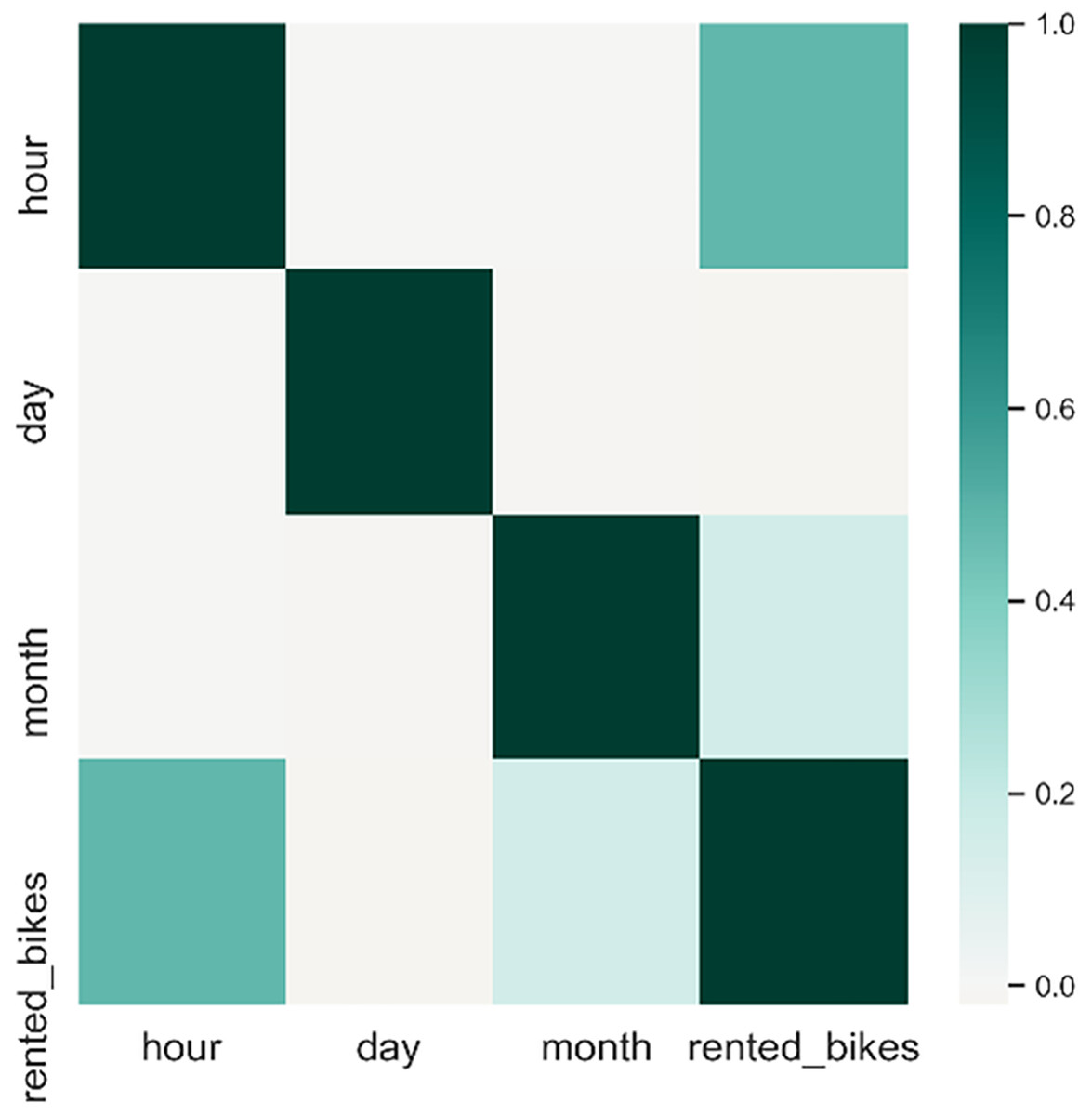
Figure 5: Pairwise correlation of all columns.
Lastly, we introduce timestamp attributes as supplementary features for the n previous values generated through the sliding window approach, encompassing elements such as the hour of the day, day of the week, and month of the year. The n previous values from the hour of the day (t), day of the week (d), and month of the year (m) are integrated with the n previous values of the counted rented bikes (c). Ultimately, given the n previous values or window size, the forecasting horizon (h), and the total data entries (N), the updated input matrix X can be formulated by creating a input matrix as can be seen in Formula (4).
(4)
Proposed MLP model
In this study, a MLP model was employed for the prediction of bike sharing demand. The MLP belongs to the category of feedforward Artificial Neural Networks (ANNs), characterized by one input layer, one or more hidden layers, and one output layer. To train the MLP, a backpropagation algorithm was utilized (Han, Kamber & Pei, 2012; Rumelhart, Hinton & Williams, 1986). Our network is fully connected, meaning each unit receives connections from all units in the preceding layer. Consequently, each unit possesses its own bias, and there exists a weight for every pair of units in two consecutive layers. The net input was computed by multiplying each input by its corresponding weight and then summing the results. Each unit in the hidden layer received a net input, which was subsequently subjected to an activation function. Therefore, with input units are denoted as , output unit as y, units in the lth hidden layer represented as , and as the activation function, the network computation can be expressed as follows.
(5)
(6)
(7)
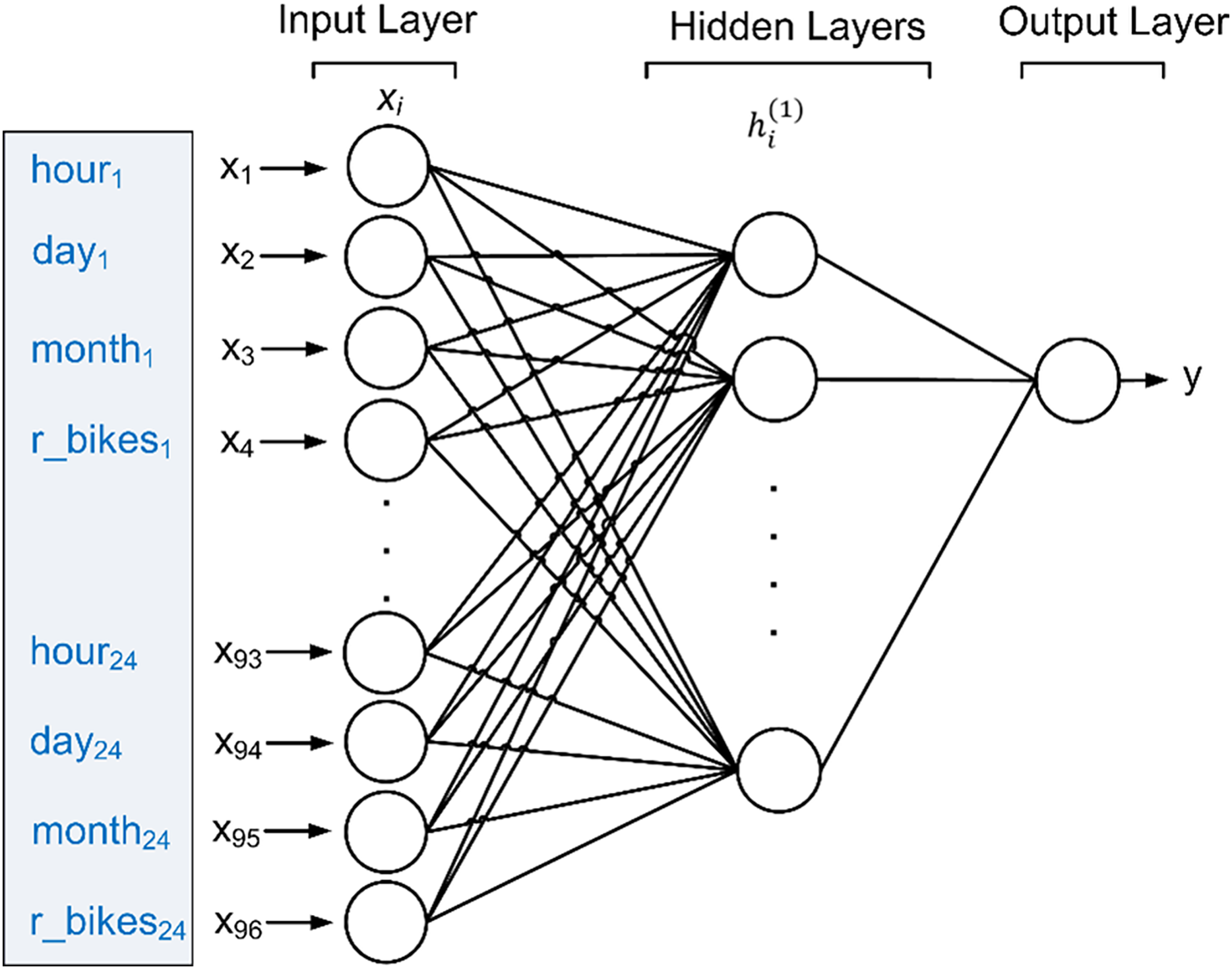
The backpropagation technique involves assessing the predicted outcome against the target value and adjusting the weights for each training tuple to minimize the mean squared error between the predicted and target values. This iterative process is repeated multiple times to achieve optimal weights, thereby enabling optimal predictions for the test data. Figure 6 depicts the suggested MLP model for forecasting the count of rented bikes, using inputs comprising the rented bikes’ history over the last 24 h, along with attributes such as the time of day, day of the week, and month of the year.
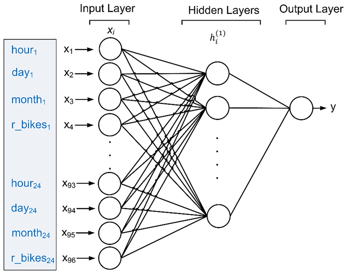
Figure 6: Proposed MLP to predict future bike sharing demand.
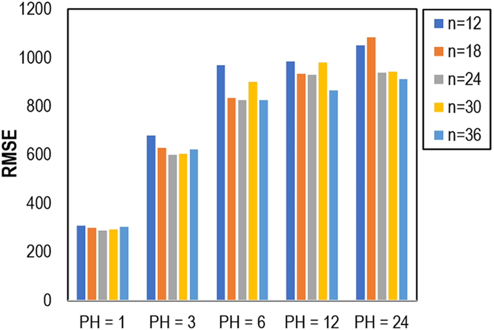
The selection of the number of lags or window size in a forecasting model is crucial as it directly impacts the prediction error. The appropriate choice of lags or window size ensures capturing relevant historical information, enhancing the model’s ability to make accurate predictions. Therefore, in this investigation, we explore the most effective window size for the proposed MLP model. Initially, we partitioned the training data (0.75 of the dataset) into an additional training set and a validation set (0.25). The MLP model underwent evaluation using various window sizes, including 12, 18, 24, 30, and 36, alongside different prediction horizons (PH) such as 1, 3, 6, 12, and 24. The outcomes of the experiment, as depicted in Fig. 7, revealed that a window size of 24 was optimal in the validation set, demonstrating lower errors for PH = 1, PH = 3, and PH = 6. Interestingly, our findings indicated that a higher window size, specifically n = 36, exhibited the lowest Root Mean Square Error (RMSE) for PH = 12 and PH = 24.
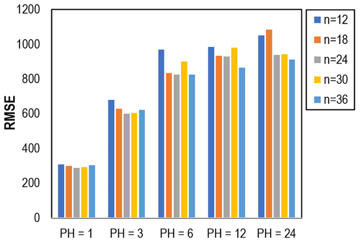
Figure 7: Impact of window size on RMSE.
Choosing the appropriate window size or number of lags in forecasting is a critical decision that significantly influences the accuracy and effectiveness of predictive models. A window size that is too small may result in overlooking important patterns and trends in the historical data, leading to an oversimplified model that fails to capture the complexity of the underlying patterns. On the other hand, an excessively large window size may introduce unnecessary noise and irrelevant information, hindering the model’s ability to discern relevant signals for prediction. Striking the right balance is essential, as an optimal window size ensures that the model leverages sufficient historical context without being overwhelmed by excessive data, ultimately contributing to more accurate and reliable forecasting results. Hence, a window size of 24 was chosen in our study as the input features for our proposed machine learning models.
The model evaluation employed the holdout method, dividing the dataset into two segments: the initial 75% for training and the remainder for testing. The forecasting models were implemented using Python V3.7.3, Scipy V1.3.2, and Scikit-learn V0.22.1 (Pedregosa et al., 2012), with optimized hyperparameters as can be seen in Table 3. Performance metrics, including RMSE, Mean Absolute Error (MAE), and Coefficient of Determination ( ), were utilized to assess the forecasting models. RMSE measures the average magnitude of differences between predicted and actual values (number of rented bikes), offering a comprehensive evaluation of prediction accuracy. MAE quantifies the average absolute differences between the predicted and actual number of bikes, providing a straightforward representation of prediction errors. Lastly, measures the proportion of variance in the dependent variable predictable from the independent variable, indicating the goodness-of-fit of the regression model.
| Regression model | Hyperparameters |
|---|---|
| MLP | 1 hidden layer with 100 nodes, 1 ouput layer with 1 node, activation function = ReLU, iteration = 1,000, weight optimization = Adam, learning rate = 0.001, batch size = 200 |
| SVR | Kernel = rbf, C = 200, epsilon = 0.2 |
| KNN | Neighbors = 5, distance metric = minkowski |
| DT | Split = mean squared error, max features = n features |
| AdaBoost | Model = Decision tree with max depth 3, number of trees = 50 |
| RF | Number of trees =100, split = mean squared error, max features = n features, bootstrap = true |
| Linear regression | Function = minimize sum squares between targets and predicted values. |
Results and discussions
Performance comparison of prediction models
The proposed MLP model was tested on the Seoul bike-sharing dataset and exhibited favorable outcomes in reducing prediction errors compared to alternative forecasting models. This research involved a comparative analysis between the proposed model and various machine learning-based prediction algorithms, including Support Vector Regression (SVR), K-Nearest Neighbour (KNN), Decision Tree (DT), Adaptive Boosting (AdaBoost), Random Forest (RF), and Linear Regression (LR). The effectiveness of each model was assessed based on lower RMSE and MAE, along with higher values in the testing sets. The predictive input features comprised the past 24 h of rented bikes to predict the next 1, 3, 6, 12, and 24 h of bike rentals. The study demonstrated that utilizing the preceding 24 h of rented bikes as input features could minimize prediction errors on the validation sets. Additionally, the proposed MLP model incorporated timestamp features (hour, day, month) as supplementary attributes, distinguishing it from other models that solely relied on the last 24 h of rented bikes for input.
Table 4 displays the average values of RMSE, MAE, and from various forecasting models aimed at predicting the demand for bike sharing (rented bikes) across different prediction horizons (PHs). The proposed MLP model demonstrated superior performance, exhibiting the lowest RMSE and MAE, as well as the highest in the testing sets compared to alternative prediction models. Specifically, the RMSE values for the proposed MLP model were 344.020, 719.812, 889.602, 920.725, and 959.997 for prediction horizons of 1, 3, 6, 12, and 24 h, respectively. Furthermore, the proposed model achieved the highest (coefficient of determination) in comparison to other models, with values of 0.973, 0.882, 0.820, 0.807, and 0.790 for PHs of 1, 3, 6, 12, and 24 h, respectively. Conversely, both Decision Tree (DT) and AdaBoost exhibited the poorest performance across all prediction horizons compared to other models. Ultimately, the findings indicated that as the prediction horizon (PH) increased, the majority of prediction models produced higher RMSE and MAE but with lower values in the testing sets.
| Model | Metrics | Prediction horizon (hours) | ||||
|---|---|---|---|---|---|---|
| 1 | 3 | 6 | 12 | 24 | ||
| SVR | RMSE | 761.924 | 948.984 | 1,037.865 | 1,111.213 | 1,067.647 |
| MAE | 458.083 | 586.341 | 649.425 | 683.296 | 674.036 | |
| 0.868 | 0.795 | 0.755 | 0.718 | 0.740 | ||
| KNN | RMSE | 679.845 | 882.159 | 999.193 | 1,050.716 | 1,186.786 |
| MAE | 452.871 | 568.127 | 632.139 | 689.973 | 786.465 | |
| 0.895 | 0.823 | 0.772 | 0.748 | 0.679 | ||
| DT | RMSE | 734.790 | 1,366.935 | 1,464.577 | 1,545.951 | 1,743.966 |
| MAE | 433.896 | 854.435 | 936.453 | 1,003.858 | 1,134.365 | |
| 0.877 | 0.574 | 0.511 | 0.455 | 0.306 | ||
| AdaBoost | RMSE | 841.109 | 1,320.566 | 1,451.032 | 1,499.690 | 1,472.425 |
| MAE | 641.504 | 1,072.684 | 1,161.608 | 1,177.256 | 1,095.239 | |
| 0.839 | 0.603 | 0.520 | 0.487 | 0.505 | ||
| RF | RMSE | 589.265 | 885.354 | 988.737 | 1,042.337 | 1,101.105 |
| MAE | 338.448 | 565.023 | 649.076 | 659.640 | 732.462 | |
| 0.921 | 0.821 | 0.777 | 0.752 | 0.723 | ||
| Linear regression | RMSE | 644.146 | 995.561 | 1,068.954 | 1,057.534 | 1,042.927 |
| MAE | 444.050 | 675.501 | 708.471 | 687.286 | 681.945 | |
| 0.906 | 0.774 | 0.740 | 0.745 | 0.752 | ||
| Proposed MLP | RMSE | 344.020 | 719.812 | 889.602 | 920.725 | 959.997 |
| MAE | 220.210 | 485.487 | 616.320 | 624.551 | 633.722 | |
| 0.973 | 0.882 | 0.820 | 0.807 | 0.790 | ||
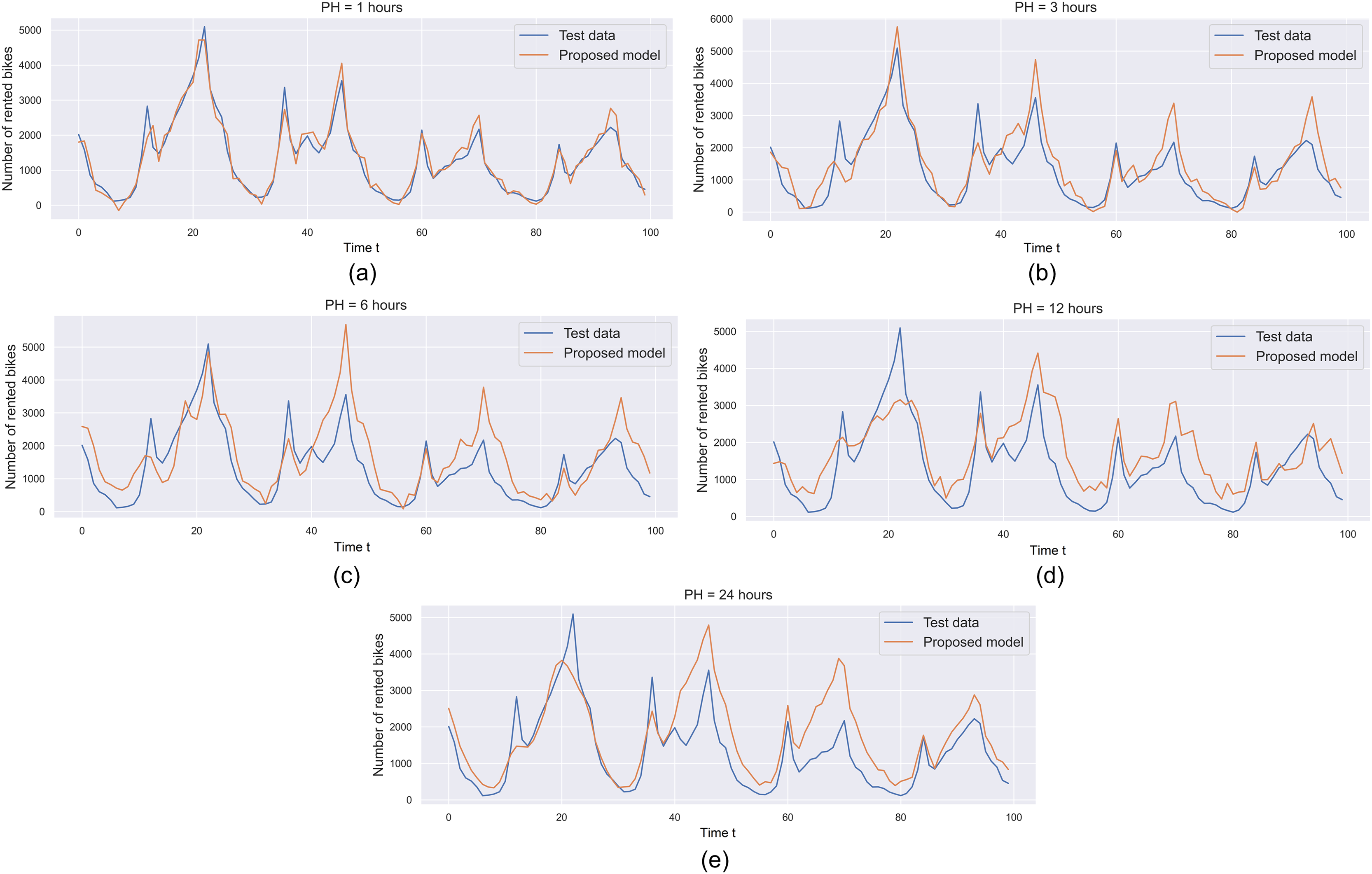
To assess the effectiveness of the suggested MLP-based prediction model, graphical representations of the prediction outputs and original values from the testing sets can be examined. As illustrated in Fig. 8, the predicted values from the proposed MLP model are visually compared with the original hourly rented bikes in the testing sets. For this graphical comparison, we opted to analyze the initial 100 points from both the testing sets and the prediction output. The findings indicate that the prediction output from the proposed MLP model closely aligns with the testing sets or original data, particularly evident with a prediction horizon (PH) of 1 h (Fig. 8A). The model’s prediction output for a PH of 1 h exhibits the lowest error when contrasted with the models for PHs of 3, 6, and 24 h. Additionally, as the prediction horizon increases, the forecasting model experiences higher prediction errors. Specifically, for a PH of 24 h (Fig. 8E), the model generates a higher error (i.e., the disparity between predicted and original values) compared to the models for PHs of 12 (Fig. 8D), 6 h (Fig. 8C) and 3 h (Fig. 8B). Based on this preliminary experiment, it can be inferred that the proposed MLP model shows great promise and could be effectively applied for predicting hourly demand in real-world bike-sharing scenarios.
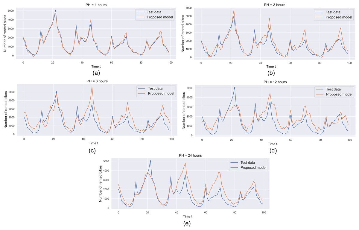
Figure 8: Predicting bike rentals with varying prediction horizon: (A) 1 h, (B) 3 h, (C) 6 h, (D) 12 h and (E) 24 h.
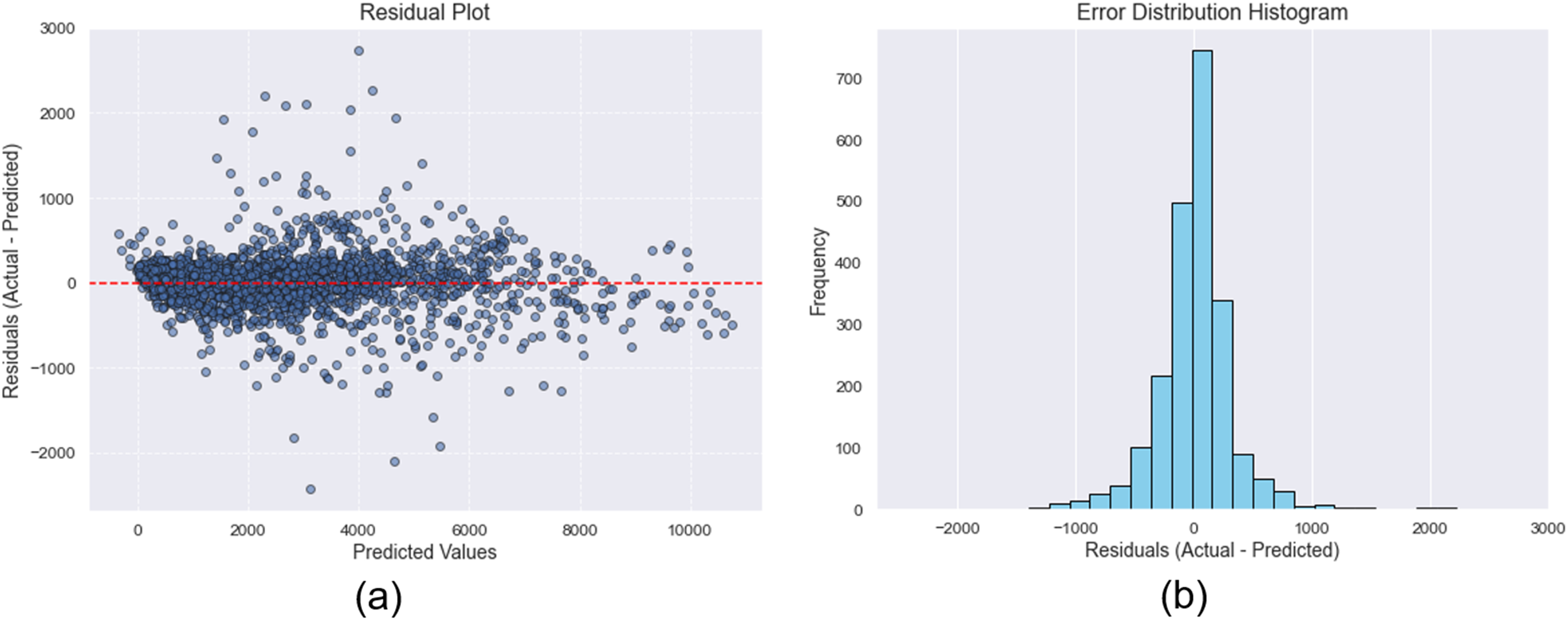
To further evaluate the predictive accuracy of the proposed model for PH = 1, a comprehensive residual analysis was conducted. The residual plot, presented in Fig. 9A, illustrates the relationship between residuals and predicted values, showing no discernible patterns or signs of heteroscedasticity. This indicates that the errors are randomly distributed, which is a desirable property in a well-performing predictive model. Additionally, the histogram of residuals in Fig. 9B reveals an approximately symmetric distribution with a slight positive skew. The descriptive statistics of the residuals are as follows: the mean residual is 11.990, indicating a negligible overall prediction bias; the standard deviation is 343.810, reflecting a moderate level of dispersion in the errors; the skewness is 0.400, suggesting mild asymmetry toward higher residual values; and the kurtosis is 10.100, indicating heavier tails than a normal distribution, which may reflect the presence of a small number of relatively large prediction errors. These results support the robustness of the model’s predictive performance and offer valuable insights into the distribution and behavior of its residuals.

Figure 9: (A) Plot of the residual errors, and (B) the histogram of the error distribution.
To determine whether the proposed MLP model provides a statistically significant improvement in performance over the baseline models, a paired t-test was carried out based on the RMSE values. As shown in Table 5, the results indicate that the proposed MLP model significantly outperforms all competing models. Specifically, the differences between the MLP and each of the baseline models—including SVR (p = 0.0153), KNN (p = 0.0092), DT (p = 0.0007), AdaBoost (p = 0.00001), RF (p = 0.0036), and LR (p = 0.0090)—are statistically significant at the 0.050 level. These findings confirm that the MLP model consistently delivers superior predictive performance, providing more accurate forecasts across all time horizons compared to the other machine learning models evaluated in this study.
| Comparison | t-statistic | p-value | Significant (p < 0.05) |
|---|---|---|---|
| Proposed MLP vs. AdaBoost | 27.93 | 0.00001 | Yes |
| Proposed MLP vs. Decision tree | 9.50 | 0.00069 | Yes |
| Proposed MLP vs. Random forest | 6.14 | 0.00358 | Yes |
| Proposed MLP vs. Linear regression | 4.75 | 0.00900 | Yes |
| Proposed MLP vs. KNN | 4.72 | 0.00917 | Yes |
| Proposed MLP vs. SVR | 4.07 | 0.01528 | Yes |
Furthermore, the proposed MLP model was evaluated against two classical statistical forecasting methods—ARIMA and Exponential Smoothing—over a 24-h prediction horizon, as can be seen in Table 6. The results demonstrate that the MLP model significantly outperforms both traditional approaches across all evaluated metrics. Specifically, the MLP achieved a RMSE of 959.997, a MAE of 633.722, and a coefficient of determination (R2) of 0.790. In comparison, the ARIMA model recorded an RMSE of 4,760.520, MAE of 3,908.360, and R2 of 0.520, while the Exponential Smoothing model achieved an RMSE of 1,571.560, MAE of 1,318.520, and R2 of 0.740.
| Model | Metrics | Prediction horizon (hours) |
|---|---|---|
| 24 | ||
| ARIMA | RMSE | 4,760.52 |
| MAE | 3,908.36 | |
| 0.52 | ||
| Exponential smoothing | RMSE | 1,571.56 |
| MAE | 1,318.52 | |
| 0.74 | ||
| Proposed MLP | RMSE | 959.997 |
| MAE | 633.722 | |
| 0.79 |
These findings indicate that the MLP model provides more accurate and reliable forecasts than the ARIMA and Exponential Smoothing models. The superior performance of the MLP can be attributed to its ability to capture complex nonlinear patterns in the data, which traditional linear models may fail to address effectively.
The impact of additional timestamp features on prediction error
Our proposed MLP-based model incorporates the previous 24 h of extracted features from timestamps as supplementary input, distinguishing it from other prediction models that rely solely on the past 24 h of rented bikes as attributes. Consequently, it is essential to investigate the impact of these additional timestamp features on the prediction error of other models. Table 7 displays the RMSE of the prediction models in the testing sets with various feature types for different prediction horizons (PHs). The outcomes reveal that the combination of the last 24 h of rented bikes and timestamp features as attributes led to lower RMSE for all PHs compared to prediction models using only previous values of rented bikes as features—except for DT (6, 12, and 24 h PHs), AdaBoost (1 and 24 h PHs), and RF (6, 12, and 24 h PHs). In the context of short-term forecasting (i.e., 1 h), the combination of rented bikes and timestamp features produced lower RMSE compared to models with rented bike attributes, except for AdaBoost. Notably, in our experimental findings, the inclusion of additional timestamp features diminished the performance of DT, AdaBoost, and RF, resulting in higher RMSE for longer-term forecasting (i.e., 24-h PH) when compared to models without timestamp features.
| Model | Feature type | RMSE | |||||
|---|---|---|---|---|---|---|---|
| Rented bikes | Timestamp | PH = 1 | PH = 3 | PH = 6 | PH = 12 | PH = 24 | |
| SVR | √ | 761.924 | 948.984 | 1,037.865 | 1,111.213 | 1,067.647 | |
| √ | √ | 674.245 | 895.855 | 987.232 | 1,054.353 | 1,006.652 | |
| KNN | √ | 679.845 | 882.159 | 999.193 | 1,050.716 | 1,186.786 | |
| √ | √ | 679.833 | 882.149 | 999.191 | 1,050.715 | 1,186.783 | |
| DT | √ | 734.79 | 1,366.935 | 1,464.577 | 1,545.951 | 1,743.966 | |
| √ | √ | 703.003 | 1,081.738 | 1,837.316 | 1,933.816 | 1,842.09 | |
| AdaBoost | √ | 841.109 | 1,320.566 | 1,451.032 | 1,499.69 | 1,472.425 | |
| √ | √ | 852.424 | 1,145.117 | 1,294.727 | 1,248.043 | 1,490.268 | |
| RF | √ | 589.265 | 885.354 | 988.737 | 1,042.337 | 1,101.105 | |
| √ | √ | 473.434 | 810.525 | 1217.227 | 1,338.149 | 1,124.303 | |
| Linear regression | √ | 644.146 | 995.561 | 1,068.954 | 1,057.534 | 1,042.927 | |
| √ | √ | 536.581 | 854.243 | 943.054 | 1,006.063 | 1,005.493 | |
| Proposed MLP | √ | 347.675 | 775.01 | 938.638 | 944.089 | 964.776 | |
| √ | √ | 344.02 | 719.812 | 889.602 | 920.725 | 959.997 | |
As depicted in Table 7, the results indicate a notable enhancement in performance by incorporating additional timestamp features, particularly for SVR and Linear Regression. The average reduction in RMSE for these models is 92.738 and 61.859, respectively, when compared to models without timestamp features. However, the impact of additional timestamp features is less favorable for the DT-based algorithms, resulting in an average RMSE increase of 108.349 compared to the non-timestamp DT model. Lastly, the proposed MLP, when augmented with extra timestamp features, has significantly lowered the RMSE by 3.655, 55.198, 49.036, 23.364, and 4.779 for prediction horizons of 1, 3, 6, 12, and 24 h, respectively, in contrast to the MLP model without timestamp features.
Comparison with previous study and other deep learning models
A prior investigation successfully demonstrated the prediction of bike-sharing demand using various models and feature types. To enhance the accuracy of hourly bike-sharing demand predictions, a Gradient Boosting Machine model was proposed in a previous study, incorporating weather and date information as input features (Sathishkumar, Park & Cho, 2020a). This model utilized the Seoul bike-sharing 2018 dataset, obtained from a Korean bike-sharing company’s reservation data spanning December 2017 to November 2018. Features in the dataset included the number of rented bikes, weather conditions, and date information for each hour.
For our experiment, we additionally employed the publicly available Seoul bike-sharing 2018 dataset from the aforementioned study and conducted machine learning-based forecasting. The input features for our proposed MLP model consisted of the last 24 h of rented bikes and timestamp information (hour, day, month). In contrast, other prediction models utilized only the last 24 h of rented bikes as input. Table 8 illustrates the averages of RMSE, MAE, and from forecasting models, focusing on predicting bike-sharing demand (rented bikes) for a prediction horizon of 1 h on the Seoul bike-sharing 2018 dataset. Notably, our proposed MLP model exhibited superior performance, yielding the lowest RMSE and MAE, as well as the highest in the testing sets when compared to alternative prediction models, including SVR, KNN, DT, AdaBoost, RF, and Linear Regression.
| Model | PH = 1 h | ||
|---|---|---|---|
| RMSE | MAE | R2 | |
| SVR | 153.146 | 98.992 | 0.939 |
| KNN | 243.977 | 158.204 | 0.845 |
| DT | 237.624 | 143.622 | 0.853 |
| AdaBoost | 256.455 | 205.907 | 0.828 |
| RF | 147.372 | 94.163 | 0.943 |
| Linear regression | 225.851 | 158.142 | 0.867 |
| Proposed MLP | 135.453 | 91.522 | 0.952 |
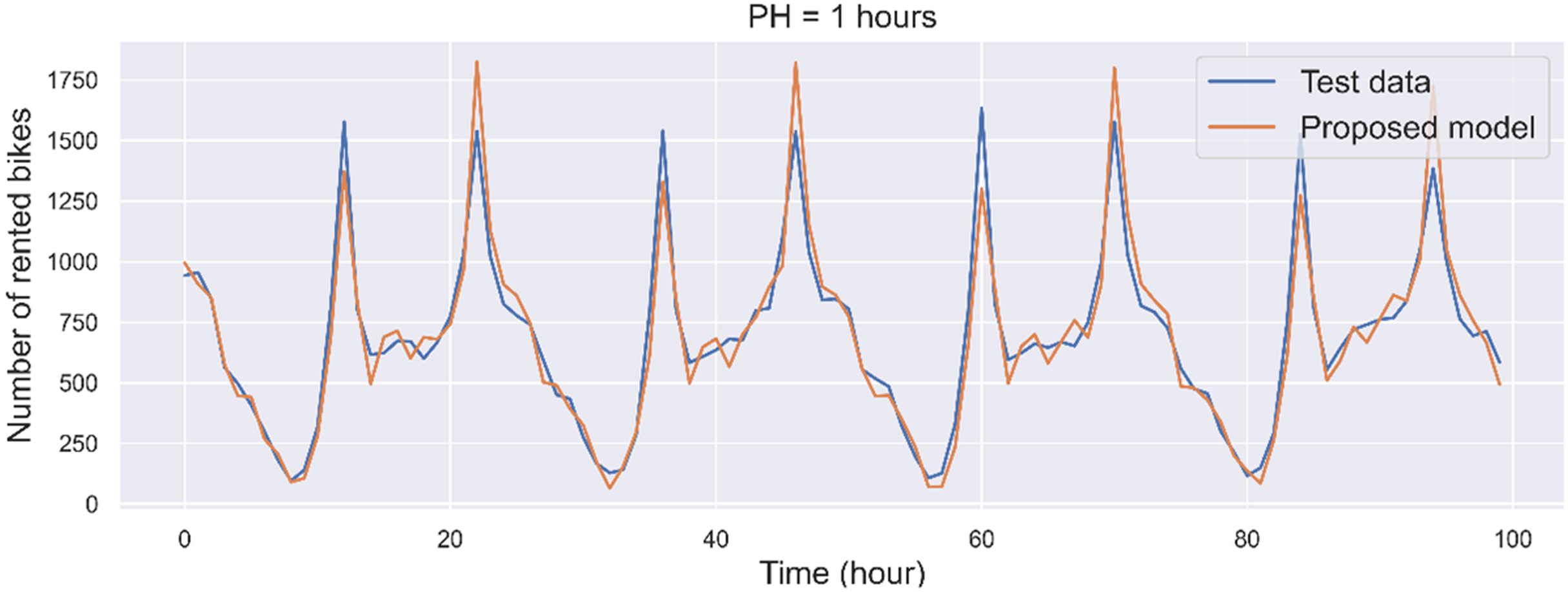
Figure 10 depicts the forecasted results produced by the proposed MLP model for a prediction horizon (PH) of 1 h. The graphical comparison includes the initial 100 points from both the testing sets and the prediction output. In terms of short-term prediction, the findings indicate that the proposed MLP model, leveraging the information from the past 24 h of rented bikes and timestamp data, can accurately predict the number of rented bikes for the following hour. The corresponding performance metrics for the proposed model are an RMSE of 135.453, an MAE of 91.522, and an value of 0.952.
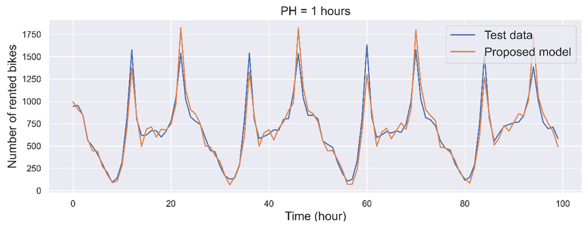
Figure 10: Forecasting of rented bikes with prediction horizon 1 h from another dataset.
We conducted a comparative analysis with a prior study on a bike-sharing demand prediction model utilizing a Gradient Boosting model (Sathishkumar, Park & Cho, 2020a). The Gradient Boosting model yielded RMSE, MAE, and values of 174.680, 109.890, and 0.920 in the testing sets, respectively. The results suggested that incorporating weather information enhanced the prediction accuracy of the models, with temperature and hour being identified as the most influential variables for hourly rented bike predictions. Unlike their approach of using current weather and date information as input features and rented bikes in each hour as the output value, our strategy involved using the previous values of rented bikes and timestamp information as input features to predict the next hour(s) of rented bikes. The RMSE, MAE, and values generated by our proposed MLP model in the testing sets are 135.453, 91.522, and 0.952, respectively. Our experiment demonstrated that by leveraging the last 24 h of rented bikes and timestamp information, the prediction of the next hour’s rented bikes can be more accurate compared to the previous study.
In our study, we exclusively utilized the most recent data on rented bikes and timestamp information as input features for machine learning models. In a real-world scenario, incorporating other inputs such as current weather conditions might be challenging, as this information must be sourced from external databases. Therefore, the objective of our work is to achieve accurate prediction outputs from models using readily available features (from bike-sharing reservation data), such as the last known information of rented bikes and timestamp information, aiming to enhance the rebalancing system for bike-sharing companies.
In addition, we compared the proposed model with approaches employed in previous studies (Boonjubut & Hasegawa, 2022; Gammelli et al., 2022; Mehdizadeh Dastjerdi & Morency, 2022; Yang et al., 2020) that utilized RNN, LSTM, and GRU. Table 9 summarizes the performance across different prediction horizons (1, 3, 6, 12, and 24 h), where the number of rented bikes in the previous hour was used as the primary input for future demand forecasting. The results clearly indicate that the proposed MLP consistently achieves lower RMSE values and higher R2 scores compared to the deep learning models.
| Model | Metrics | Prediction horizon (Hours) | ||||
|---|---|---|---|---|---|---|
| 1 | 3 | 6 | 12 | 24 | ||
| LSTM | RMSE | 585.146 | 995.501 | 1,072.019 | 1,170.162 | 968.125 |
| R2 | 0.922 | 0.774 | 0.738 | 0.688 | 0.786 | |
| GRU | RMSE | 394.343 | 955.413 | 1,209.051 | 1,023.806 | 984.149 |
| R2 | 0.965 | 0.792 | 0.667 | 0.761 | 0.779 | |
| RNN | RMSE | 425.899 | 873.487 | 951.088 | 1,009.451 | 969.495 |
| R2 | 0.959 | 0.826 | 0.794 | 0.768 | 0.785 | |
| Proposed MLP | RMSE | 344.020 | 719.812 | 889.602 | 920.725 | 959.997 |
| R2 | 0.973 | 0.882 | 0.820 | 0.807 | 0.790 | |
The superior performance of the MLP can be attributed to the integration of temporal attributes in addition to lagged demand values. By incorporating features such as hour of the day, day of the week, and month of the year through a sliding window approach, the model effectively captures daily commuting cycles, weekly usage patterns, and seasonal variations. These findings demonstrate that with well-designed feature engineering, a relatively simple MLP can outperform more complex recurrent architectures. While LSTM and GRU are effective in modeling sequential dependencies, their performance may be limited when temporal context is not explicitly represented. By combining lag sequences with timestamp-based features, the proposed MLP achieves a strong balance between simplicity and predictive accuracy, highlighting its practical applicability for both short-term operational decisions and long-term strategic planning in bike-sharing systems.
Conclusions and future works
In this study, we introduced a forecasting model based on a MLP designed to predict the upcoming hour(s) of bike-sharing demand. We employed a direct strategy to transform time-series data into a set of paired inputs and corresponding desired outputs. The dataset was compiled from customer reservation data in 2020 from a bike-sharing company in Seoul, Korea. To enhance prediction accuracy, we utilized the last 24 h’ data on rented bikes and timestamp information as input features for the proposed MLP. Our MLP model demonstrated superior performance, yielding the lowest RMSE and MAE, and the highest compared to alternative prediction models. The results indicated that accurately predicting the next hour of rented bikes is achievable by leveraging the last 24 h’ data on rented bikes and timestamp information, with RMSE, MAE, and values of 344.020, 220.210, and 0.973, respectively. Furthermore, a comparison with a previous study, using a publicly available dataset, showcased improved prediction accuracy in our model.
This study was based on data from a single bike-sharing company in Seoul, limiting the generalizability of the model’s performance. Investigating various multi-step forecasting strategies and using a broader set of evaluation metrics could offer a more comprehensive performance assessment. Additionally, exploring alternative imputation methods may improve accuracy, especially with more complex or incomplete data. Incorporating multi-task learning to jointly predict related outcomes could enhance generalizability. Lastly, evaluating model performance across different temporal segments and applying cross-validation would strengthen robustness and highlight time-specific trends.