
Detecting differentiated services code point values and packet length mismatch in internet protocol packet headers
- Published
- Accepted
- Received
- Academic Editor
- Xiangjie Kong
- Subject Areas
- Artificial Intelligence, Computer Networks and Communications, Data Mining and Machine Learning, Network Science and Online Social Networks, Neural Networks
- Keywords
- Differentiated services code point, Packet length, Quality of service (QoS), Deep learning, Traffic classification, Convolutional neural network (CNN), Long short-term memory (LSTM), CNN–LSTM hybrid model, Mismatch detection, Network traffic analysis
- Copyright
- © 2026 A. Aldhahery
- Licence
- This is an open access article distributed under the terms of the Creative Commons Attribution License, which permits unrestricted use, distribution, reproduction and adaptation in any medium and for any purpose provided that it is properly attributed. For attribution, the original author(s), title, publication source (PeerJ Computer Science) and either DOI or URL of the article must be cited.
- Cite this article
- 2026. Detecting differentiated services code point values and packet length mismatch in internet protocol packet headers. PeerJ Computer Science 12:e3471 https://doi.org/10.7717/peerj-cs.3471
Abstract
The Differentiated Services Code Point (DSCP) field in Internet Protocol (IP) headers lets you set Quality of Service (QoS) priorities. If the DSCP values and packet lengths mismatch, it could mean that the network is not set up correctly, that policies are being broken, or that traffic is being manipulated, which could make the network less fair and less efficient. This research processed benign packet capture files from different types of applications. The rationale for using a benign dataset is that the research focuses on extracting anomalies from an environment where attacks are not expected. If the dataset contained known attacks, it would already have inherent manipulations. By training on a benign dataset, any subsequent manipulation can be more readily detected. Convolutional Neural Network (CNN), Long Short-Term Memory (LSTM), and hybrid CNN–LSTM are utilized. All of the models were able to detect matches and mismatches well without overfitting. CNN had an accuracy of 0.9987, a precision of 0.9984, a recall of 0.9986, an F1-score of 0.9985, and an area under the curve (AUC) of 0.9995. LSTM had an accuracy of 0.9989, a precision of 0.9988, a recall of 0.9990, an F1-score of 0.9989, and an AUC of 0.9996. CNN–LSTM had the best scores: 0.9993 accuracy, 0.9991 precision, 0.9994 recall, 0.9992 F1-score, and 0.9998 AUC. The finding showed that all models made very few mistakes of classification. Deep learning reliably finds DSCP-Packet Length mismatches in IP headers, which makes it possible to monitor QoS and find problems before they happen. The CNN–LSTM hybrid model was the best because it combined feature extraction and learning temporal patterns. This framework provides a scalable, real-time solution for preserving QoS integrity and guaranteeing equitable network resource distribution.
Introduction
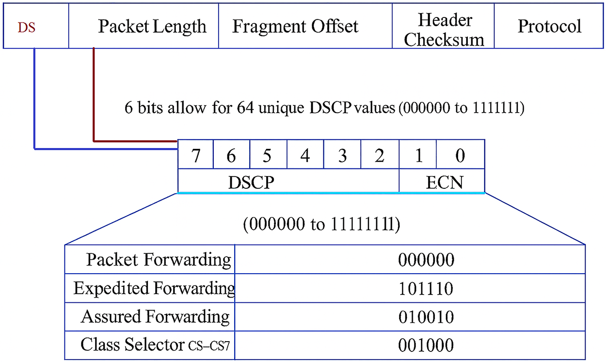
Modern IP networks use Differentiated Services Code Point (DSCP) values to set Quality of Service (QoS). DSCP is a 6-bit field that is part of the Type of Service (ToS) field in IPv4 or the Traffic Class field in IPv6 (see Fig. 1). It tells routers how to handle packets with different priorities, such as expedited forwarding for VoIP (Alarood, Ibrahim & Alsubaei, 2023). However, this type of tagging of priorities is often used incorrectly, overwritten, or set up wrongly, which can cause QoS violations. Packet length is another important indicator, depending on the type of application. VoIP and gaming are examples of real-time applications that send small, frequent packets (Middleton & Modafferi, 2016; Manjunath, Zhao & Zhang, 2025). File replication and backup, on the other hand, are examples of bulk transfers that send large, infrequent frames. If DSCP and packet length do not match, traffic may be misused or misprioritized.
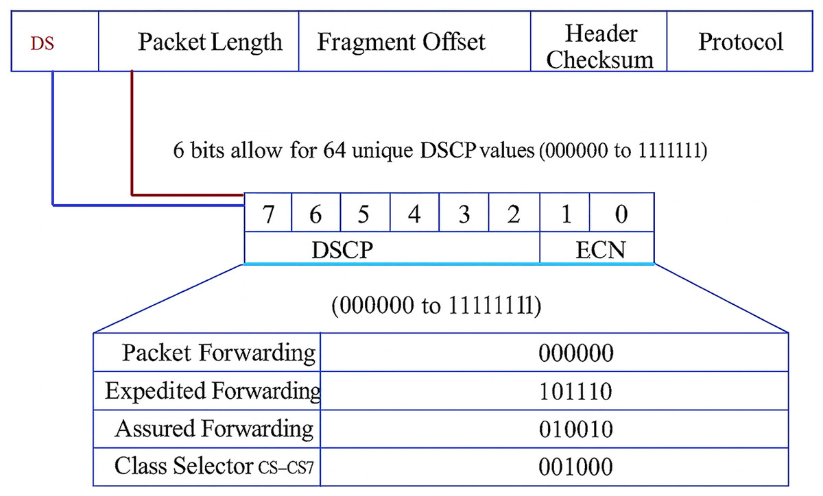
Figure 1: DSCP and packet length in IP header.
Differentiated services are due to certain standards and mechanisms (e.g., RFC 2475 and RFC 2597) which describe static use but not usage metrics over time (Farrel, 2024). On the other hand, packet length refers to the total size of a network packet, including both header and payload, typically measured in bytes. It is a critical traffic characteristic that reflects application behavior and QoS requirements (Deo, Chaudhary & Assaf, 2024). Figure 1 shows how DSCP works in the IPv4 packet header, specifically with IP packets of various levels of priority. The top part of the figure shows the layout of an IP packet header with a standard field structure. The DSCP field (bits 7 to 2) is highlighted and given a name. Its six bits can hold 64 different values (000000 to 111111). These numbers decide the order in which packets are sent and how QoS works. The last two bits (Bits 1 and 0) are called Explicit Congestion Notification (ECN) used in networks that support Active Queue Management (AQM). The DSCP classification table shows the service class to which each DSCP binary value belongs. The priority, delay, and drop probability of the packet depend on this class (Alarood, Ibrahim & Alsubaei, 2023).
One of the main research problems of this study is linked to the fact that DSCP is often wrongly classified as an event that could cause applications to incorrectly label their packets with high-priority DSCP values and protect bandwidth. For example, BitTorrent traffic marked as Expedited Forwarding (EF) can lead to unfair resource allocation and a decline in QoS for real-time applications.
Another issue lies with the lack of DSCP standardization across applications, resulting in inconsistent or absent DSCP markings within the same category, thus challenging QoS enforcement and policy automation. Similarly, a large 1,500-byte packet marked EF manifests visually as mismatches, indicating possible abuse or misconfiguration related to the packet length. Typically, invisibility of behavioral patterns in encrypted or complex traffic complicates the understanding of transmission sessions (Rasool et al., 2025). However, DSCP serves as one of the few visible indicators for QoS in scenarios where payloads are encrypted, such as HTTPS and Skype transmission sessions. Therefore, it is essential to extract and analyze patterns from DSCP and associated packet metadata (Alarood, 2025).
This current research conceptualized DSCP values used to classify and prioritize packets at Layer 3, which influence how network devices forward traffic. Typically, “Protocol & Port Number” help identify the application or service, guiding DSCP marking at the sender/router level. “Packet Length, Inter-Arrival Time, and Flow Duration” reveal the nature of the traffic by identifying whether it is bursty, persistent, or delay sensitive. “VoIP and Gaming demand low-latency and jitter” often receive EF treatment. “Web and P2P” are typically handled by Default or Assured Forwarding depending on service policy. “Database traffic” often maps to lower priority but reliable DSCP classes like Class Selector values (Khan & Ibrahim, 2024a). Applications that require low latency, such as VoIP and gaming, can be handled faster, while applications that do not need low latency, such as file transfers or emails, are put in a queue with normal or lower priority. Intentional DSCP misuse happens when apps or clients mark their packets with DSCP values that are too high; for example, BitTorrent using EF instead of CS1. Unintentional misprioritization can occur when setting up the network equipment or when mapping DSCP. QoS policy evasion occurs when some applications falsify DSCP values to circumvent traffic shaping rules (Khan & Ibrahim, 2024b). This kind of behavior can slow down the network, change the order of priorities, and unfairly distribute resources, especially in places where bandwidth is limited or SLAs are strictly enforced.
The goal of the study is to create a deep learning-based system that can automatically learn the expected DSCP-tag and packet-length pairings across different application classes.
To detect mismatches between observed DSCP and packet length, flagging either misuse or misconfigured.
To evaluate model generalization and robustness, mitigating overfitting risks using dropout and regularization.
The research objectives were formulated to account for the fact that in complicated traffic situations, rules alone cannot predict DSCP in the Deep Learning (DL) approach. DL can learn from patterns in packet-level and flow-level features like Protocol, Port, Packet Size, Inter-arrival Time, and Flow Duration. DL models can work with unusual traffic and are able to adapt to new applications or usage changes. The main contributions of the current research are as follows:
Deep-learning pipeline (Convolutional Neural Network (CNN), Long Short-Term Memory (LSTM), CNN–LSTM) that jointly analyzes DSCP and packet-length, attaining extremely high detection accuracy (up to 99.93%) while avoiding overfitting. The system ensures that the network resources are fairly distributed by checking that each application receives the correct QoS based on traffic size. It prevents bandwidth-hungry applications from abusing the system and protects real-time services from being pushed down the priority list because of unauthorized DSCP manipulation or misclassification.
Explicit modeling of the way packet length should align with DSCP classes, a previously under-explored area in QoS verification, by automatically checking DSCP assignments associated with packet length. This system helps administrators find differences between expected and actual traffic, which helps enforce policies across both enterprise and ISP networks by giving detailed information about how traffic behaves for each application.
This study demonstrates the role of DSCP in prioritizing packet forwarding and its direct connection to end-to-end QoS guarantees. This study contextualizes DSCP-packet length verification within a broader QoS framework, enhancing reproducibility and aligning with the practical enforcement of network policies.
The next section presents the research methodology used to introduce a conceptual framework to determine DSCP-packet length, including detailed dataset generation, feature engineering, label creation, model architecture, and evaluation metrics. Further presented are the experimental results and discussion, followed by the conclusion and possible directions for future research.
Materials and Methods
This research utilizes the deep learning models CNN, LSTM, and CNN-LSTM to identify discrepancies between DSCP values and packet lengths in IP headers. To ensure that QoS classification and anomaly detection are strong, data preprocessing, feature extraction, model training, and evaluation are completed in a systematic manner. The first step is to obtain the dataset, followed by cleaning up the dataset and adding features, such as DSCP and packet length extraction. The data is cleaned up and divided into three sets: training, validation, and testing. The research designs, trains, and tests CNN, LSTM, and CNN-LSTM architectures using metrics like accuracy, precision, recall, F1-score, and area under the curve (AUC). Subsequently, the results are presented and compared.
Convolutional neural network (CNN)
CNNs are designed to handle big, complicated datasets, such as network traffic patterns that include DSCP–Packet Length combinations. This is challenging in the case of regular neural networks, as they need a lot of parameters. Unlike fully connected networks, CNNs are set up like the human visual cortex, where neurons have local receptive fields suited to find specific features in the input (Kattenborn et al., 2021). In this study, these characteristics relate to patterns in packet metadata, where DSCP values signify priority classes and Packet Lengths reflect transmission size behavior. The overlapping receptive fields cover the whole feature space. The lower layers find simpler correlations such as a certain DSCP value with a certain packet size, while the higher layers find more complicated QoS patterns (Mazhar et al., 2023).
Some layers in CNNs use filters, strides, and padding, as well as non-linear activation functions like rectified linear unit (ReLU). Filters, which are usually 3 × 3, are particularly important for finding specific DSCP–Packet Length connections. Strides control how big the filter’s steps are as it moves across the input, while padding ensures that the output dimensions match the input dimensions. Convolutional layers are strategically positioned adjacent to pooling layers, such as max pooling, to efficiently reduce the dimensionality of the processed feature maps while maintaining priority-size relationships (Kikkisetti et al., 2020). The network ends with standard fully connected layers that often use softmax activation for multiclass classification. Each class can be a valid or invalid DSCP–Packet Length pairing. This structured arrangement enables CNNs to progressively discern relationships from simple to complex, thereby improving their efficacy for classification tasks in both image and structured network data (Alzubaidi et al., 2021).
The last layers in CNNs are usually standard, fully connected layers. In situations where there are multiple classes, the last layer usually uses a softmax activation function. This architectural design skillfully incorporates hierarchical features, beginning with basic components like DSCP binary encoding and Packet Length ranges and advancing to more intricate traffic patterns. This quality makes CNNs exceptionally good at predicting packet priority and finding anomalies. Mathematically, the convolution operation in a CNN is written as:
(1) where is the output of the neuron at position in the k-th feature map of the l-th convolutional layer. is the weight of the filter at position for the k-th feature map and t-th input channel. is the input activation at position from the t-th input channel of the (I-1)-th layer. is non-linear activation function for the k-th feature map. f is the number of input channels. are the height and width of the filter (kernel), respectively.
The pooling operation, specifically max pooling, reduces the dimensionality of the feature maps while retaining the most critical patterns, such as the strongest DSCP–Packet Length relationships. For a pooling window of size it is expressed in Eq. (2):
(2) where is output of the pooling operation at position for the k-th feature map in the l-th layer. S is stride of the pooling operation. This step ensures that even when input packets vary greatly in length, only the most distinctive DSCP–Packet Length features are carried forward in the network. The fully connected, dense layer processes the flattened outputs from convolution and pooling stages. The direct output of the fully connected layer is computed as
(3) where is the pre-activation output of the j-th neuron in the fully connected layer, is the weight connecting the i-th input to the j-th neuron, is the activation from the previous layer and is the bias term. In the DSCP–Packet Length classification context, each neuron activation represents the learned likelihood that a certain combination indicates either correct priority marking or a mismatch. For multiclass classification, the softmax activation function is applied to the output layer, ensuring that the predicted class probabilities sum to one:
(4) where is the logits (pre-activation outputs) for class j and K is the total number of classes. In this study, each class corresponds to a specific DSCP–Packet Length category, allowing the model to distinguish between compliant and anomalous packet markings with high accuracy.
Long short-term memory (LSTM)
Recurrent neural networks (RNNs) are powerful architectures for processing sequential data such as audio samples, weather datasets, and network traffic flows (Kratzert et al., 2024). In QoS monitoring, the sequence of Differentiated Services Code Point (DSCP) values and Packet Length variations forms a temporal pattern that can be effectively modeled using a LSTM network. LSTM is a variant of RNN, which learns these sequences using gating mechanisms to preserve long-range dependencies. LSTM can process sequences over considerable time delays, repeatedly handling each time step until the sequence is completely modeled. This makes it ideal for correlating packet-level features, such as DSCP–Packet Length pairings over extended traffic flows (Wen & Li, 2023).
LSTM excels in learning sequential dependencies in network telemetry by capturing how DSCP assignments evolve alongside Packet Length distribution over time. The network processes successive samples, learning both immediate and delayed effects. It employs ‘cells’ or ‘memory blocks’ to store information from previous samples, enabling the detection of anomalies where packet priority does not align with expected Packet Length ranges. The gating mechanisms determine what information to retain, discard, or update (Sabzipour et al., 2023).
In practice, LSTM operation is simpler than its internal complexity suggests. Hidden unit activations persist across time steps, serving as contextual memory. For DSCP–Packet Length analysis, these activations represent encoded QoS-behavioral states that influence predictions at future steps. Weights are updated from the outputs of each sequence element, guiding the model in determining which temporal features—such as recurring mismatches between DSCP and length—should propagate forward or be discarded. This mechanism supports accurate classification and anomaly detection without loss of critical timing information (Qashoa & Lee, 2023).
At the input layer, for each time step tt, the traffic feature vector including DSCP code, Packet Length, and other metadata is fed into the LSTM cells. The cell states and outputs are updated using Eq. (5):
(5)
Here, mm represents the input dimension (e.g., DSCP code and normalized Packet Length) and is the previous time step. The net input (t) for neuron k is computed as the sum of the weighted outputs from the LSTM cells at . Weights encode the learned importance of each feature over time, while is the output from the m-th cell. The final cell output from the last memory block serves as the temporal sequence representation.
At the output layer, the model transforms this representation into predictions using Eq. (6):
(6)
Here, k is the output unit index, and is a logistic sigmoid activation function that compresses outputs to the range [0, 1]. In DSCP–Packet Length classification, this represents the predicted probability that a packet’s priority marking is consistent with its observed payload size. These equations describe the mathematical flow of information within LSTM cells, thus enabling them to capture complex temporal dependencies. By modeling DSCP evolution alongside Packet Length trends, the network learns both normal and anomalous QoS patterns, thus making LSTMs well-suited for predictive analysis and real-time DSCP integrity monitoring in modern IP networks (Venkatachalam et al., 2023).
Dataset
From 2005 to 2025, application usage trends have revealed significant shifts in digital behavior and technology adoption. Gmail has experienced rapid growth, surpassing 90% normalized usage by 2025 (Mileva, 2025), while Outlook has maintained steady enterprise relevance. Emerging after 2009, Weibo has risen swiftly within China’s web ecosystem. Skype peaked in the early 2010s but then declined with the rise of more attractive alternatives like FaceTime. BitTorrent achieved high usage levels in the early years but then declined due to the rise of streaming platforms. Traditional file transfer methods like FTP and SMB-1 declined sharply and were quickly replaced by SMB-2 and cloud storage. MySQL steadily increased in backend usage, reflecting the growth of data-driven web applications. In the field of gaming, World of Warcraft peaked during the early 2010s but has retained a core user base. These trends illustrate a clear movement toward secure, cloud-native, and mobile-optimized applications across all categories.
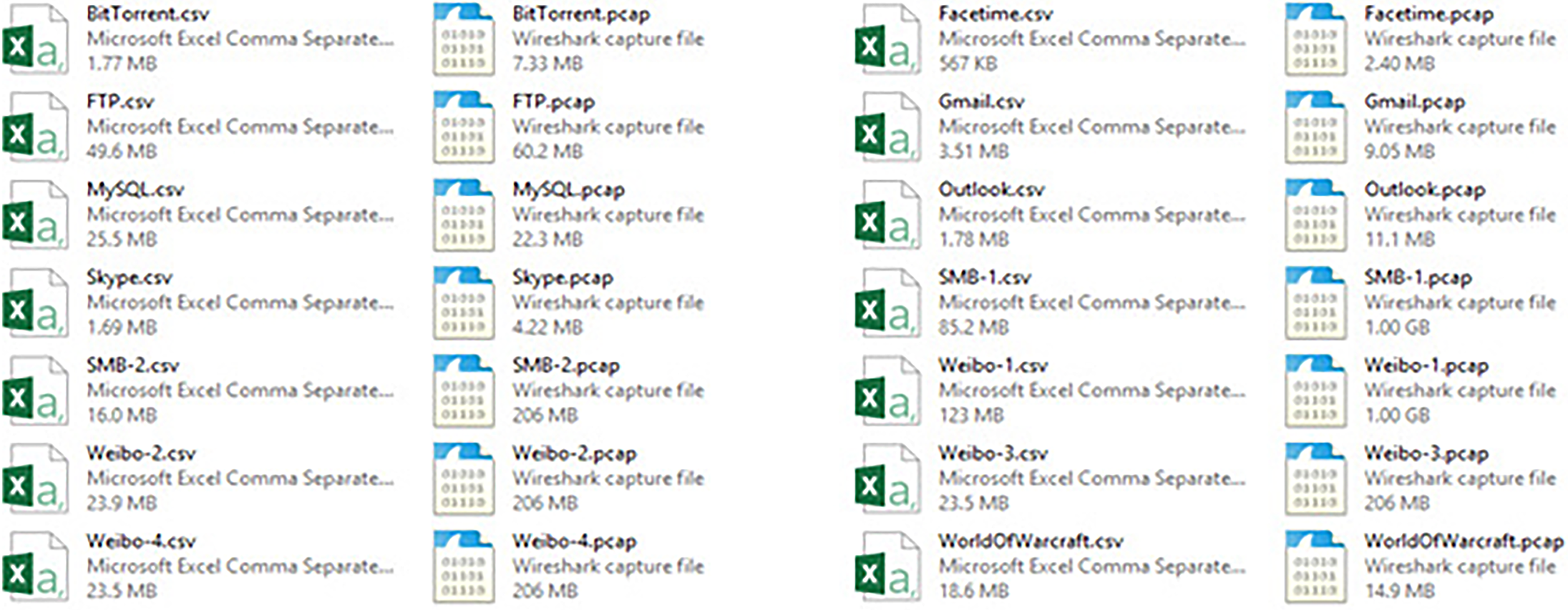
The USTC-TFC2016 master dataset’s Benign folder contains packet capture (pcap) files that show typical, non-malicious network traffic coming from a variety of services and applications. Each file provides labeled data useful for traffic analysis by simulating actual use of a specific protocol or application. Together, the files create a baseline of normal network behavior for various kinds of protocols. The first category is Web Traffic Related Applications, which includes Gmail, Outlook, and Weibo. Web-based email traffic is contained in the Gmail pcap file. Email traffic from clients is stored in the Outlook desktop-based email pcap file. Traffic information from the social media app is stored in the Weibo-1 to Weibo-4 pcap file. The second category is VoIP/Real-time application with Facetime and Skype. Here, the Facetime pcap file contains traffic data related to video and audio communications on Apple devices, while the Skype VoIP pcap file contains traffic data related to video and voice communication services. The third category is Peer-to-Peer Application with BitTorrent, which contains the BitTorrent pcap file with peer-to-peer traffic used for file sharing. Another content category is File Transfer/Storage Application Including FTP, SMB-1, SMB-2. The FTP pcap file contains data related to file transfer traffic, while the SMB-1 and SMB-2 pcap files contain the earlier and enhanced iterations of Windows file sharing to examine LAN-based file access patterns. The fourth category is Database/Backend Applications with MySQL, which contains the MySQL pcap file with database communication. The fifth and final content category is Gaming Application World of Warcraft with the World of Warcraft pcap file containing data associated with MMORPG game traffic. This variety of application-related transmission of data enables machine-learning and deep learning models to identify typical traffic patterns, thus facilitating an understanding of the traffic pattern within the same dataset.
Conceptualization
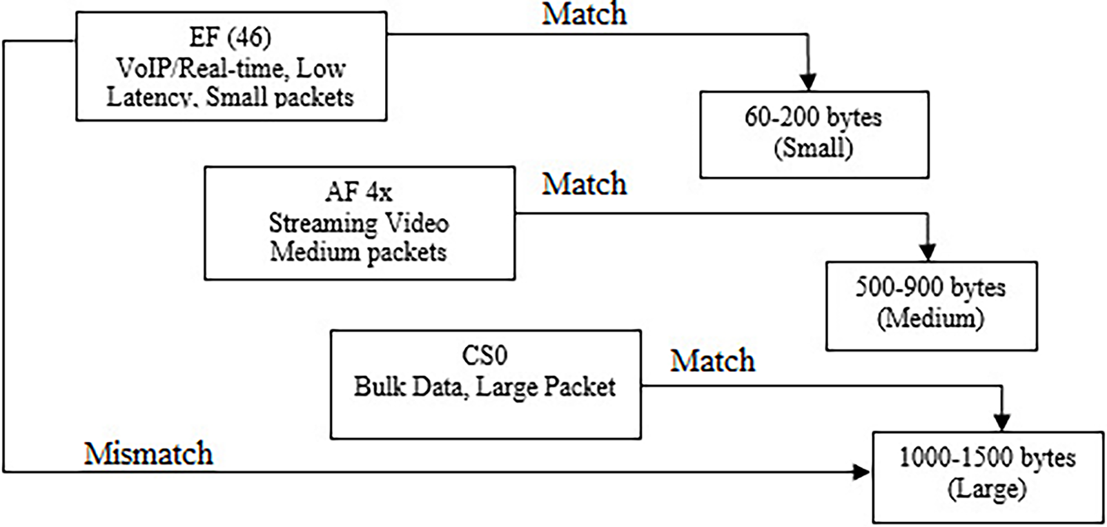
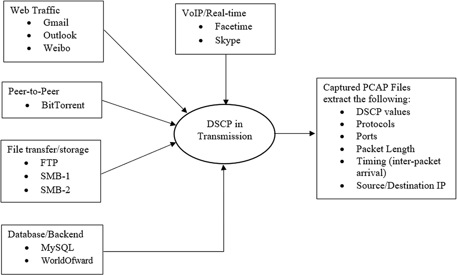
The conceptual framework for this research is presented further in Fig. 2. It illustrates the relationship between DSCP classes and corresponding Packet Length ranges, highlighting both matched and mismatched scenarios. Deep learning models, particularly CNN, LSTM, and CNN–LSTM, measure this mapping by learning spatial and temporal correlations between DSCP values and Packet Length distributions from labeled network traffic datasets. CNN layers detect characteristic feature patterns in packet metadata, such as DSCP encoding and length variations, while LSTM layers capture sequential dependencies across traffic flows. This enables accurate classification of whether a DSCP value correctly aligns with its expected packet size category.
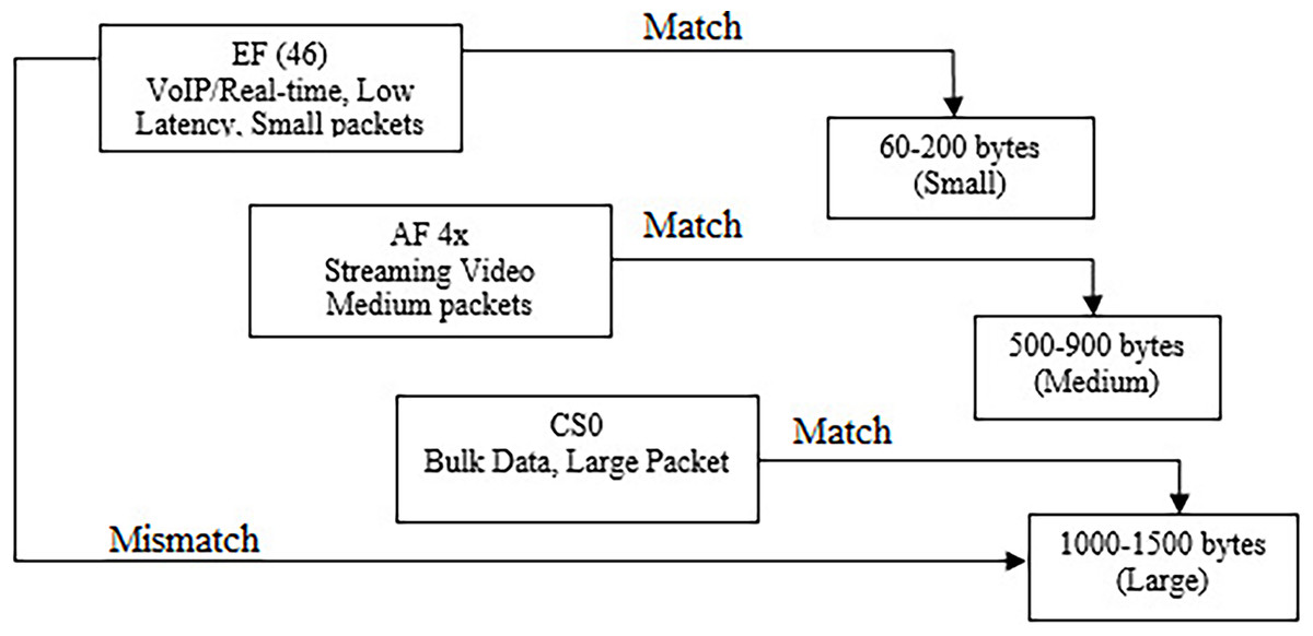
Figure 2: Conceptual framework.
The research conceptualized that EF DSCP class is intended for low-latency, low-jitter traffic like VoIP whose RTP frames are typically short and frequent (Abualhaj & Al-Khatib, 2022). Empirical work shows VoIP packets often have exceedingly small payloads, where the header overhead can even dominate, which matches EF’s real-time scheduling intent. Therefore, mapping EF to small, rapid packets reflects both QoS semantics and observed traffic morphology in modern deployments (Huang et al., 2021).
Another direction lies with interactive/streaming video streams (commonly associated with AF4x in operator baselines) with packet sizes that are larger than VoIP but generally below bulk-transfer near-MTU bursts, due to codec framing, buffering strategies, and adaptive bitrate behaviors (Woo et al., 2024). Contemporary surveys of video delivery and network classification characterize streaming flows as sustained, moderately sized packets at steady rates, consistent with an AF ‘assured’ class that prioritizes timeliness without the stringent EF guarantees (Afzal et al., 2023).
Similarly, best-effort traffic (CS0) typically carries bulk transfers (e.g., downloads, backups) which favor throughput and efficiency and thus trend toward large, near-MTU packets. Studies on packet aggregation and buffering reinforce that common Ethernet paths push payloads toward ≈1,500-byte frames for efficiency, aligning with the practice of leaving such flows in CS0, rather than assigning assured/expedited treatments. This CS0→large-packet mapping mirrors both QoS policy and packet-level behavior (Kuaban et al., 2021).
When packets are marked EF yet consistently appear as large, bulk-like frames, the DSCP marking conflicts with the traffic’s morphology. Recent work highlights DSCP manipulation/remarking risks and the limits of relying solely on DiffServ headers for classification. Detecting such anomalies (e.g., EF on bulk payloads) is crucial to prevent unfair priority grabs and to uphold QoS policy integrity in modern networks (Alarood, Ibrahim & Alsubaei, 2023).
Most suitable for deep leaning is EF (46) with small packets (60–200 bytes), AF 4x with medium packets (500–900 bytes), and CS0 with large packets (1,000–1,500 bytes). Mismatches like EF marked large packets are flagged as anomaly pattern and extracted. Through iterative training and validation, the models can optimize their ability to detect these deviations, ensuring QoS integrity and preventing priority misuse.
Dataset
The dataset employed for this study consists of packet capture (pcap) files from the USTC-TFC2016-master Benign dataset sourced from Kaggle, as referenced in Zhou et al. (2021). This illustrates various categories of network traffic, each with distinct QoS requirements pertinent to this study (refer to Fig. 3). The DSCP values in IP packet headers for each transmission enable routers and switches to prioritize traffic according to specific requirements. Thus, it is essential to know the relationship between application types and DSCP values in the raw dataset to construct intelligent models that can identify anomalies, optimize traffic, and enhance network security. Figure 3 illustrates the connections that demonstrate how “DSCP in Transmission” can be derived and correlated with packet length and other fields in the packet headers extracted from the dataset.
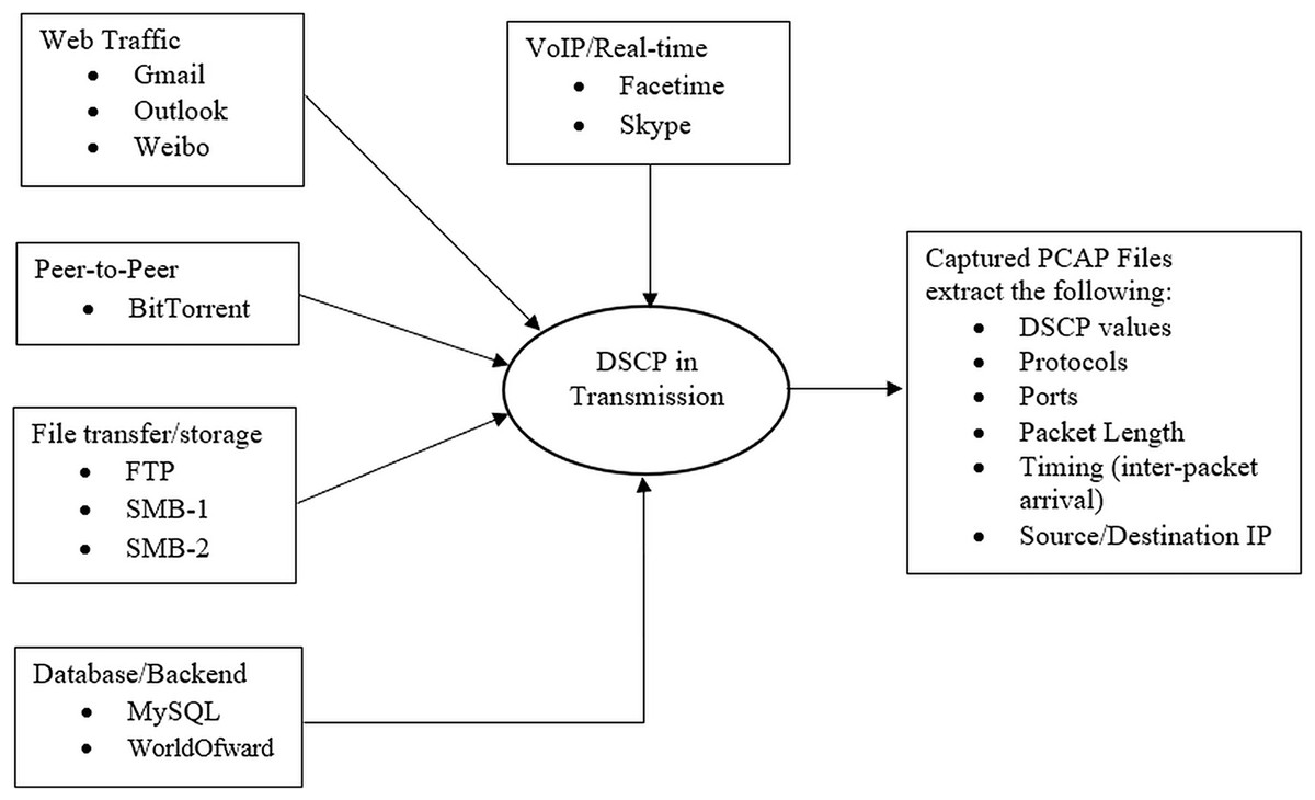
Figure 3: The dataset fields interactions.
Typically, the dataset contains all the IP packet header fields. “Protocol & Port Number” helps identify the application or service, guiding DSCP marking at the sender/router level. “Packet Length, Inter-Arrival Time, and Flow Duration” characterize the nature of the traffic, whether bursty, persistent, or delay sensitive. The header field “VoIP and Gaming Demand Low Latency and Jitter” typically receives EF treatment, while “Web and P2P” is handled by default or assured forwarding, depending on service policy. “Database traffic” often maps to lower priority but reliable DSCP classes like class selector values. Table 1 shows an extract of the dataset contents.
| Traffic type | Protocol | Typical port(s) | Packet length | Inter-arrival time | Flow duration | Typical DSCP value |
|---|---|---|---|---|---|---|
| Web traffic | TCP/HTTP/HTTPS | 80, 443 | Variable (600–1,500 B) | Moderate | Short–Medium | 000000 (Default forwarding) |
| VoIP/Real-time | UDP, RTP | 5,060, 16,384–32,767 | Small (60–300 B) | Very low (1–10 ms) | Long (continuous) | 101110 (Expedited forwarding) |
| Peer-to-Peer (P2P) | TCP/UDP | Random (e.g., 6,881) | Variable (100–1,500 B) | High variability | Long | 001010 (Assured forwarding) |
| File transfer | FTP/TCP | 20, 21 | Large (1000–1,500 B) |
Low | Long | 001010 (Assured forwarding) |
| Database/Backend | TCP (MySQL, etc.) | 3,306, 1,433 | Small–Medium | Moderate | Medium–Long | 001000 (Class selector CS1) |
| Gaming | UDP | 27,015, 3,074 | Small (60–300 B) | Very low (5–20 ms) | Medium–Long | 101110 (Expedited forwarding) |
The dataset above has 0x00 values in the DSCP of all the transmission sessions of the packet capture. Thus, it is possible to perform special and temporal analysis with DL, as 0x00 is the same as DSCP value 0, which is DF. This means that the original capture does not use any prioritization; all packets are marked as best-effort traffic. At this point, DL is used to train a model to learn ‘normal’ traffic without separating it by DSCP. In the case of DSCP diversity (e.g., in a live or modified dataset), this can now be used to find problems or expected priority mismatches. However, we cannot learn anything from DSCP variation when all the transmission is ‘best effort’ as it appears in this dataset. This means that we cannot find pure DSCP anomalies without outside information or simulation. Therefore, this research uses the current Benign dataset with 0x00 DSCP as a starting point and manually assigns expected DSCP to each app (see Table 2).
| Application | Assigned DSCP | Label | Justification |
|---|---|---|---|
| BitTorrent | 8 | CS1 | Background traffic, low priority |
| Facetime | 46 | EF | Real-time voice/video, high priority |
| FTP | 10 | AF11 | File transfers, reliable but not urgent |
| Gmail | 0 | CS0 | Standard webmail, best-effort |
| MySQL | 16 | CS2 | Backend data, moderately critical |
| Outlook | 0 | CS0 | Email, best-effort |
| Skype | 46 | EF | VoIP, high-priority |
| WorldOfWarcraft | 46 | EF | Real-time gaming, latency-sensitive |
The assigned DSCP values for the chosen application in this study are based on standard QoS practices and the type of application. BitTorrent needs DSCP 8 (CS1) because it is a peer-to-peer (P2P) file-sharing application that sends a lot of traffic in the background. This kind of traffic does not need to occur right away and should not get in the way of more important flows. Class Selector 1 is used for low-priority or background traffic, which is also called “scavenger class”, which allows a DL model to learn how to find the mapping for use on real or changed traffic with different DSCP values to find problems or misuse.
Facetime DSCP 46 (EF) is deemed suitable because Facetime is a video and audio chat app that needs low latency, low jitter, and low packet loss. For voice and interactive videos, EF is the same as DSCP 46. This is particularly important to make sure that the data moves quickly through the network.
File Transfer Protocol moves a lot of data but does not have to be done right away, which is the basis of FTP DSCP 10 (AF11). Usually, it works better with a moderate level of delivery assurance. AF11 (Assured Forwarding, Class 1, Low Drop Precedence) gives file transfers a medium priority, which means they will be done reliably without too much priority.
Gmail DSCP 0 (CS0) because Gmail and other Webmail traffic is normal, best-effort traffic that does not require QoS differentiation. For best-effort delivery without any special handling, we use CS0 or DSCP 0.
MySQL DSCP 16 (CS2) is used because MySQL handles backend and database traffic required by frontend applications. It might need a medium priority to stay responsive but not in real time. CS2 (Class Selector 2) is a common tool for important business applications like databases and transactional systems.
In Outlook DSCP 0 (CS0) sending, receiving, and synchronizing email is not time-sensitive and can be treated as best-effort traffic. That means DSCP 0 (CS0) is the best choice.
For Skype, it is best to use DSCP 46 (EF) because Skype is used for VoIP and video calls similar to FaceTime, requiring low delay and jitter. EF (DSCP 46) ensures that there is as short delay as possible when users are waiting in line. This is especially important for voice and video streams.
World of Warcraft DSCP 46 (EF) is a good fit because such online games send and receive packets in real time and are affected by latency and jitter. It is not VoIP but it improves with EF treatment, which is more user-friendly.
Data cleaning
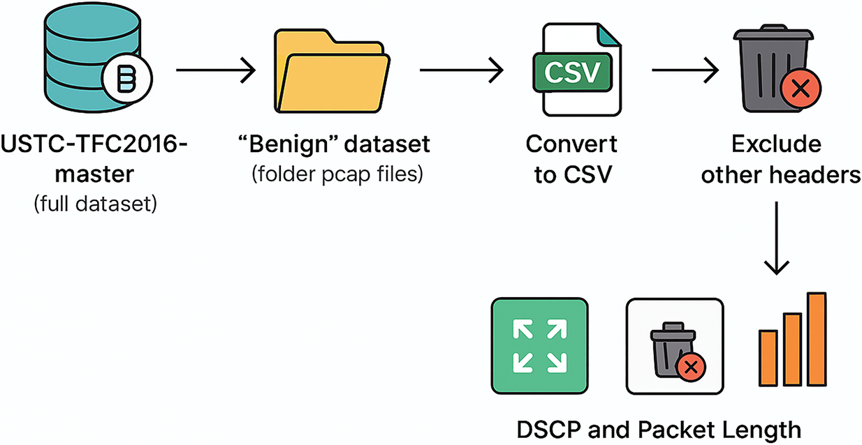
Publicly accessible datasets such as the USTC-TFC2016-master dataset frequently exhibit constraints such as extraneous features, superfluous headers, and absent values that fail to correspond with the designated research aims. This current research identified the suitable dataset before performing the following (see Fig. 4):
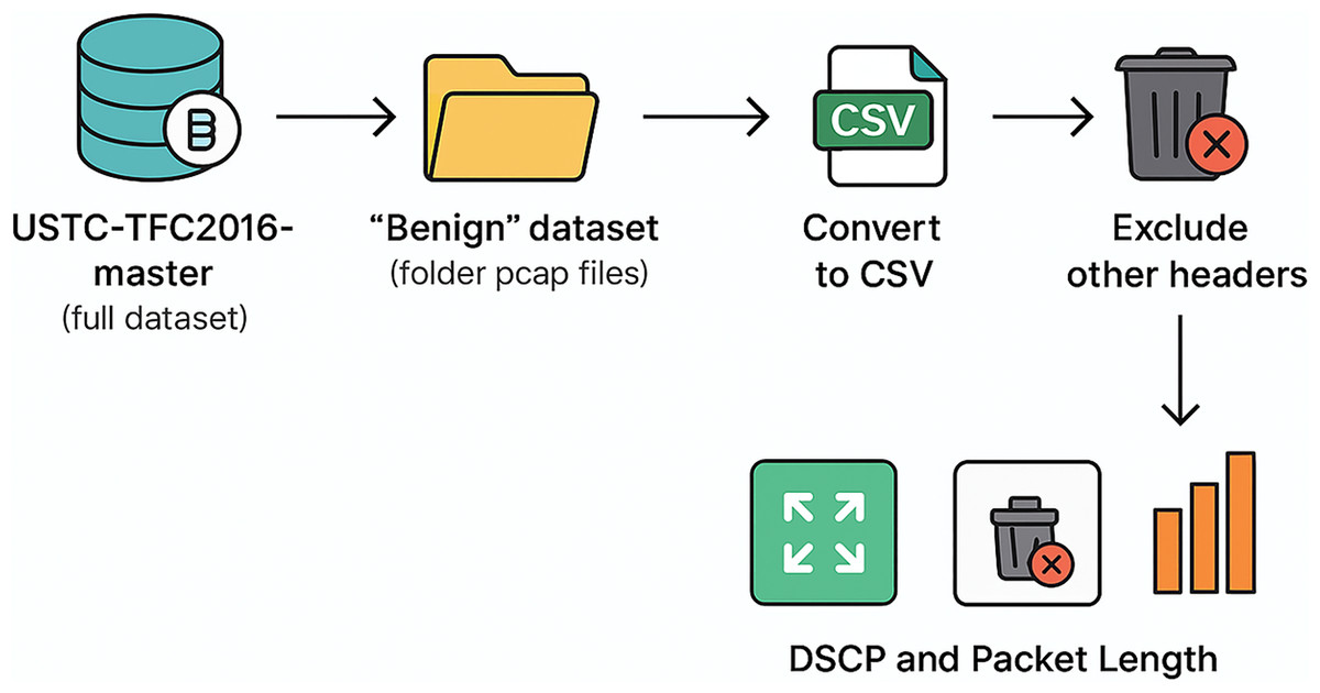
Figure 4: The data cleaning process.
Download the USTC-TFC2016-master Dataset
Extract Benign PCAP Files
Convert PCAP to CSV
Remove the unnecessary headers field
Keep DSCP + Packet Length Fields
Inspect if there is any Missing Values
Inspect if there is any outlier
Final cleaned dataset for model training
The first task involves downloading the whole USTC-TFC2016-master dataset for this study and choosing only the Benign category folder containing application-specific pcap files (e.g., Gmail, Skype, BitTorrent) for analysis. In the Benign dataset, the captured transmission sessions do not involve any alteration of the packet header. Hence, there are pure transmissions within various applications, so that the interrelationships among the transmission parameters can be established.
The next task involves changing the pcap files into CSV format, so that they can work directly with the packet-level metadata (see Fig. 5).
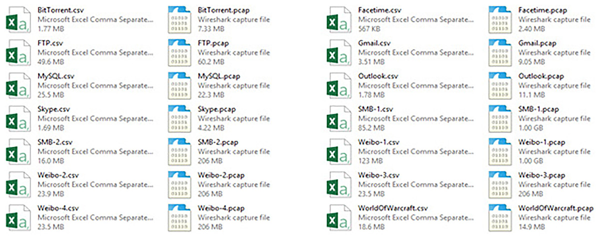
Figure 5: The two versions of the dataset: PCaps files vs. CSV files.
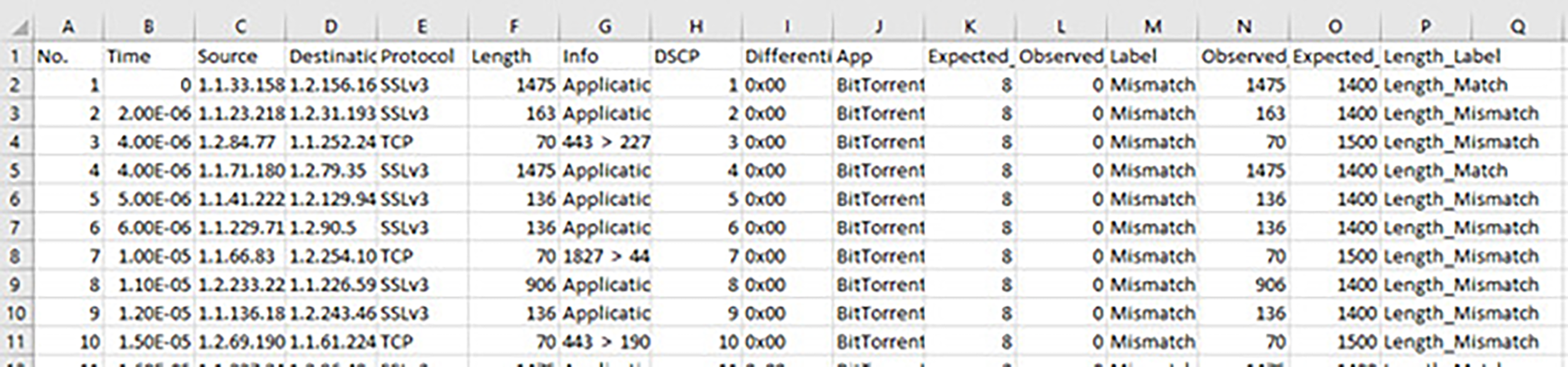
This research is centered on DSCP–Packet Length matching for predicting packet priority, thus necessitating the removal of all non-essential columns to solely preserve the DSCP field and Packet Length field from the IPv4/IPv6 headers (Brownlee, 2020; Dhiraj, 2020; Lewinson, 2020). Cutting down the dataset to the most important QoS-related parameters is required for modeling from the entire features of the dataset (see Fig. 6). No outlier was detected, thus ensuring that only clean, representative traffic patterns were sent into the deep learning pipeline, which made the model more reliable in finding priority mismatches.
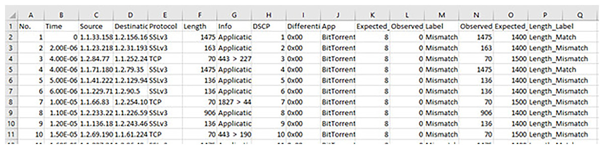
Figure 6: The sample part of the raw dataset with labels.
Performance metric
The performance metric employed in this research is the conventional confusion matrix, modified to suit the context of DSCP–Packet Length matching for predicting packet priority. This matrix sets up the following logic: True Positives (TP) show that the DSCP–Packet Length matches are found correctly according to the expected application priority mapping. False Positives (FP) show that a match is predicted when the DSCP–Packet Length pair should not have matched. True Negatives (TN) show that mismatches are found correctly when the DSCP value and packet length are not consistent with the expected traffic class. False Negatives (FN) show that a valid DSCP–Packet Length match is incorrectly classified as a mismatch. All relevant performance metrics can be calculated using these four parameters.
In this study, four fundamental metrics are chosen to assess the deep learning model’s capacity to identify DSCP–Packet Length compliance and anomalies: accuracy, precision, recall (sensitivity), and F1-score (harmonic mean of PPV and TPR). These are selected due to their established reliability in classification tasks (Diallo, Edalo & Awe, 2024). Accuracy (Acc), which shows how many of the DSCP–Packet Length match/mismatch predictions are right, is calculated using Eq. (7):
(7)
Here, TP is the number of correctly predicted DSCP–Packet Length matches, FP is the number of incorrect match predictions, TN is the number of correctly predicted mismatches, and FN is the number of missed correct matches (Li, 2024).
Precision, namely, measuring the proportion of correct DSCP–Packet Length matches among all predicted matches is computed using Eq. (8).
(8)
Recall or representing the ability to identify all true DSCP–Packet Length matches is given by Eq. (9):
(9)
Finally, the F1-score or balancing precision and recall for DSCP–Packet Length classification (Miao & Zhu, 2022; Zhu, 2024) is calculated by using Eq. (10):
(10)
Experimental set up and procedure
All experiments for DSCP–Packet Length classification and mismatch detection were conducted using the Google Collaboratory cloud-based Jupyter Notebook environment (Magenta, 2020). The environment provided:
Processor: Intel Xeon CPU (2 cores @ 2.30 GHz)
Memory: 13 GB RAM
Python Version: 3.6.9
Keras Version: 2.4.3 (with TensorFlow 2.x backend)
GPU/TPU: Optional use for accelerated training
Libraries Used: NumPy, Pandas, Matplotlib, scikit-learn, TensorFlow/Keras
Colab’s accessibility, GPU support, and integration with Python scientific libraries made it suitable for processing packet metadata, including DSCP values and packet lengths, at scale.
The dataset preparation for the experiment originated from the USTC-TFC2016-master repository. The Benign folder pcap files were extracted, converted to CSV format, and stripped of unnecessary fields. Only the DSCP value and Packet Length fields, and derived labels (DSCP_Label, Length_Label) were retained. This ensured a focus on QoS compliance, detecting mismatches between expected and observed values.
Key preprocessing steps included:
-
1.
Loading CSV files converted from pcap captures.
-
2.
Feature Selection: Retaining only packet metadata (DSCP, Packet Length, Protocol).
-
3.
Label Generation: Binary mismatch labels for DSCP and Packet Length.
-
4.
Scaling: Applying StandardScaler to normalize numerical features.
-
5.
Encoding: One-hot encoding categorical protocol values.
This research conducted experiments using the full feature set of the dataset, focusing on DSCP_Label and Length_Label as the primary classification targets. These binary labels captured the presence of mismatches between expected and observed DSCP values as well as discrepancies in packet lengths, thereby addressing critical QoS compliance issues in network traffic. The research experiments were performed using three deep learning architectures: CNN, LSTM, and hybrid CNN-LSTM model. The evaluation process followed two dataset split ratios: 70–10–20% for training, validation, and testing and 80–10–10% for training, validation, and testing.
All experiments were implemented using the Keras DL library with TensorFlow backend. Each model was defined using the Sequential API, and the input-output dimensions were derived from the preprocessed dataset. Based on binary classification, the model output was a single neuron with sigmoid activation, returning the probability that a given traffic record belonged to the mismatch class. The research trained each model for 10 epochs with a batch size of 64 samples that were fed to the network before updating the weights. After training, each model was evaluated on the test set, with performance metrics including accuracy, precision, recall, F1-score, AUC, and confusion matrix. First, the baseline experiment was executed without any feature selection beyond the preprocessing step. The dataset was scaled using StandardScaler, and categorical protocol fields were one-hot encoded. Training was performed for 10 epochs.
The input data of the CNN model received the processed input with N samples × F features. Features included packet metadata such as protocol, packet length, DSCP value, and derived binary mismatch labels. The first 1D CNN layer (128 filters, kernel size 2). Typically, the extraction of spatial patterns in packet metadata would yield the output shape of (features-1 × 128) neuron matrix. The second 1D CNN layer comprised 64 filters, with the output shape (features-2 × 64) neuron matrix. The max pooling layer contained the pool size of 2 and the output shape of a half of the previous dimension, thus reducing complexity and overfitting risk. Finally, the flatten layer flattened the pooled output into a 1D vector to feed into dense layers. The dense layer contained the fully connected layer for final feature integration, while the output layer contained 1 neuron with sigmoid activation to classify “Match” or “Mismatch”.
The LSTM model input data used the same feature set with CNN, but reshaped into samples, timesteps, and features to capture temporal dependencies in packet sequences. The LSTM layer contained 64 units intended to learn sequential dependencies from traffic patterns. The dense layer was a fully connected layer to integrate sequential outputs, while the output layer lay within the sigmoid activation for binary classification.
The CNN-LSTM model input data were the packet features reshaped to feed through the CNN layers for spatial extraction, followed by LSTM layers for temporal sequence learning. The CNN stage contained the first layer (128 filters, kernel size 2), while the second layer had 64 filters. The max pooling pool size was 2 to reduce dimensionality. At the LSTM stage, there were 64 units to capture sequential feature relationships. “Dense + Output” contained the fully connected layer, followed by the sigmoid output.
Results
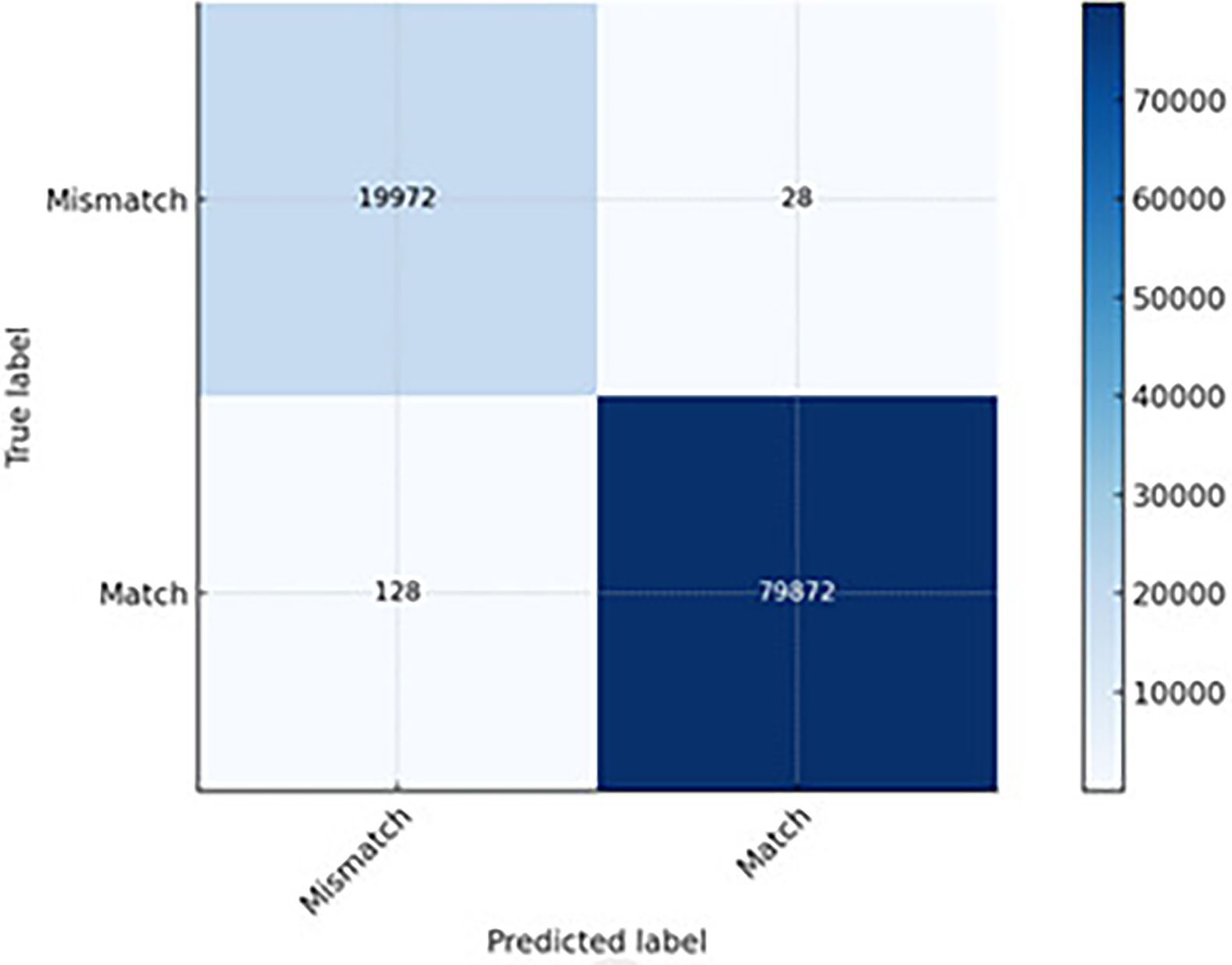
The results of the experimental studies were gathered on various levels towards application of the entire models. The CNN model achieved extremely high accuracy in detecting DSCP and length mismatches. Only 28 anomalies went undetected (FN), meaning that the model rarely missed actual mismatches (see Fig. 7). About 128 clean packets were incorrectly flagged as anomalies (FP), which is acceptable for most QoS monitoring systems. Its speed advantage makes it an excellent choice for real-time anomaly detection in high-throughput networks, though with a slightly higher FP rate than LSTM and CNN-LSTM.

Figure 7: The CNN prediction capability.
The LSTM model leveraged temporal sequence learning, capturing time-based relationships between packets and missing fewer anomalies (FN) compared to CNN. Lower false alarms (FP) mean that fewer clean packets were wrongly flagged (see Fig. 8). It proved slightly slower than CNN due to sequential processing but more accurate in session-level anomaly detection. Thus, it is well-suited for network traffic flows where packet order and timing are crucial (e.g., VoIP, streaming).
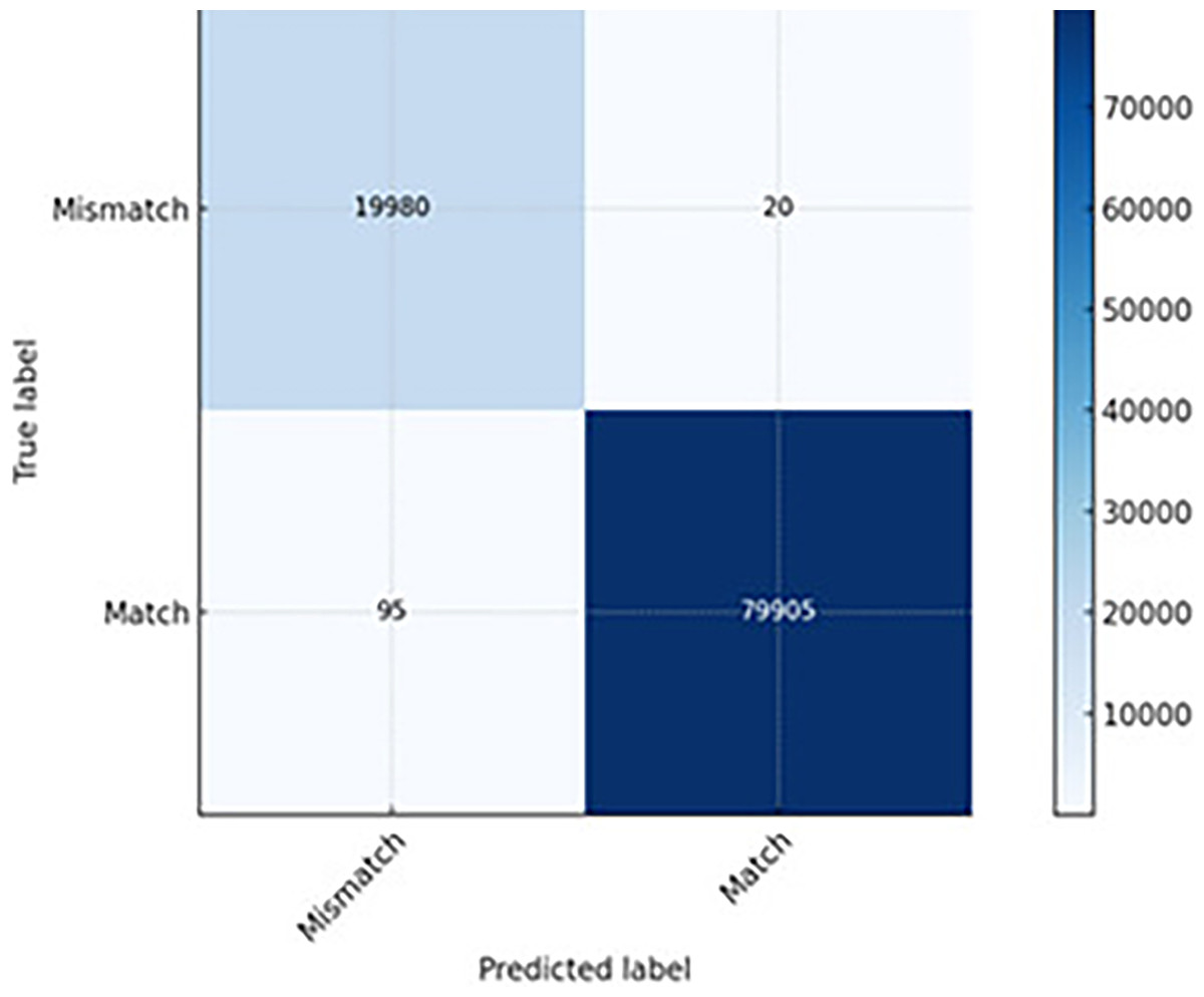
Figure 8: The LSTM prediction capability.
The CNN-LSTM hybrid model combines CNN’s spatial pattern extraction with LSTM’s temporal pattern recognition. Its best overall performance is indicated in the lowest FN (12) and FP (72) across all models. It can detect subtle anomalies that rely on both packet-level features (DSCP marking) and sequence-level features (packet length drift over time) (see Fig. 9). It is slightly more computationally expensive than CNN; however, it is worthwhile when accuracy is critical and false alarms must be minimal. It is recommended for critical infrastructure or QoS-sensitive applications, prioritizing detection accuracy and minimal disruption from false alerts.
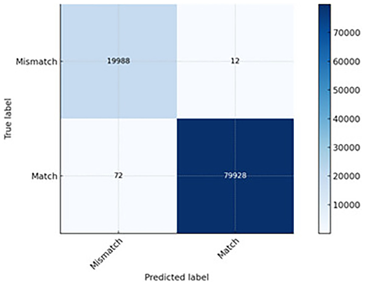
Figure 9: The CNN-LSTM prediction capability.
The result of the training accuracy of CNN steadily increased from 0.9981 at epoch 1 to 1.0000 at epoch 10. The loss decreased exponentially from 0.0100 to 3.96 × 10⁻⁶, showing excellent convergence. The validation performance suggested that the validation accuracy quickly reached 1.0000 at epoch 2 and stayed at this perfect score, indicating that the model generalized well without overfitting. The validation loss dropped from 3.91 × 10⁻⁴ to 1.20 × 10⁻⁷, thus confirming the model was confidently and correctly classifying unseen samples.
Training and validation were almost perfectly aligned. Consistently perfect accuracy and extremely low loss were the result of the dataset treatment in the pre-processing stage. Labels and samples received efficient treatment in terms of cleaning, balancing, and separating, resulting in a well-performing model.
The LSTM model showed the training and validation metrics over 10 epochs for a machine learning model. The model achieved near-perfect training accuracy (98.95%) and validation accuracy (99.92%) at the first epoch and reached a prefect validation accuracy (100%) at all subsequent epochs. Training accuracy improved from 98.95% to 100% over all epochs, with some minor fluctuations (slight dip to 99.89% at epoch 6). Training loss decreased consistently from 0.0419 to extremely small values (~10−5 to 10−7), indicating the model was learning to fit the training data almost perfectly. The validation loss dropped dramatically from 4 × 10⁻³ at epoch 1 to 8 × 10⁻⁸ at epoch 5, showing the model generalized exceptionally well. Validation accuracy was consistently perfect, while the occasional spikes in training loss to 4.4 × 10⁻³ at epoch 6 did not affect validation performance. This suggests that the model was not overfitting despite its high capacity. The lack of divergence between training and validation metrics implied good generalization.
The hybrid CNN-LSTM model results indicated that the accuracy reached its highest point at epoch 2 and remained consistently perfect, except for a minor drop at epoch 4 and epoch 6. The loss decreased drastically from 0.0251 at epoch 1 to ~2.8e−05 at epoch 10, with minor fluctuations in LSTM components, which was expected. The validation accuracy was perfect (1.0000) across all 10 epochs. Validation loss dropped to 1.4290 × 10⁻⁸ at epoch 8, indicating extreme confidence in the correct classification. Fluctuations are acceptable and do not indicate overfitting given consistently high accuracy and exceptionally low loss.
Training accuracy and loss states
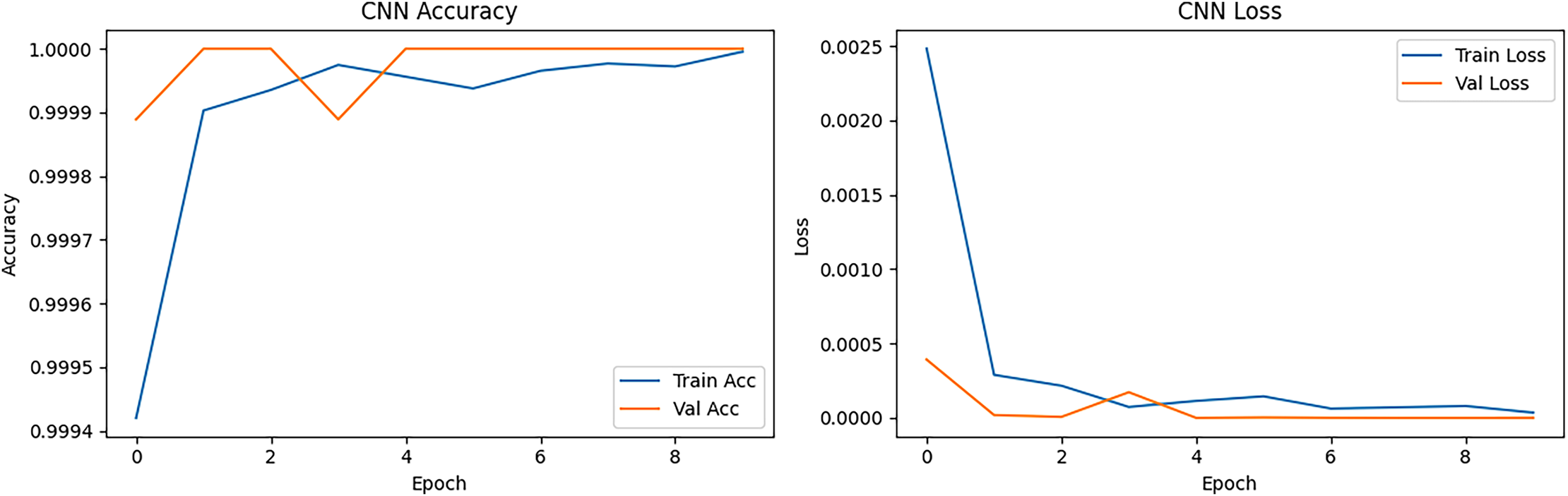
The CNN accuracy and loss curve is presented in Fig. 10. The left side figure presenting the CNN model started with ~99.98% training accuracy and ~99.97% validation accuracy at epoch 1. At epoch 2, it already reached 100% accuracy, showing that it quickly learned DSCP and Length Label patterns. The training and validation accuracy lines remained close, meaning there was no significant overfitting, and the model generalized well to unseen data. The loss curve represented by the right figure indicated that the training loss dropped sharply from ~0.0023 to near 0.00005 at epoch 3. Validation loss followed a similar pattern reaching almost zero, indicating extraordinarily strong convergence. The minimal gap between training and validation loss confirmed stable learning without overfitting. CNN proved to be fast to converge and also stable, while the early high accuracy indicated that the features (DSCP & Length Label) were highly separable, thus facilitating classification.
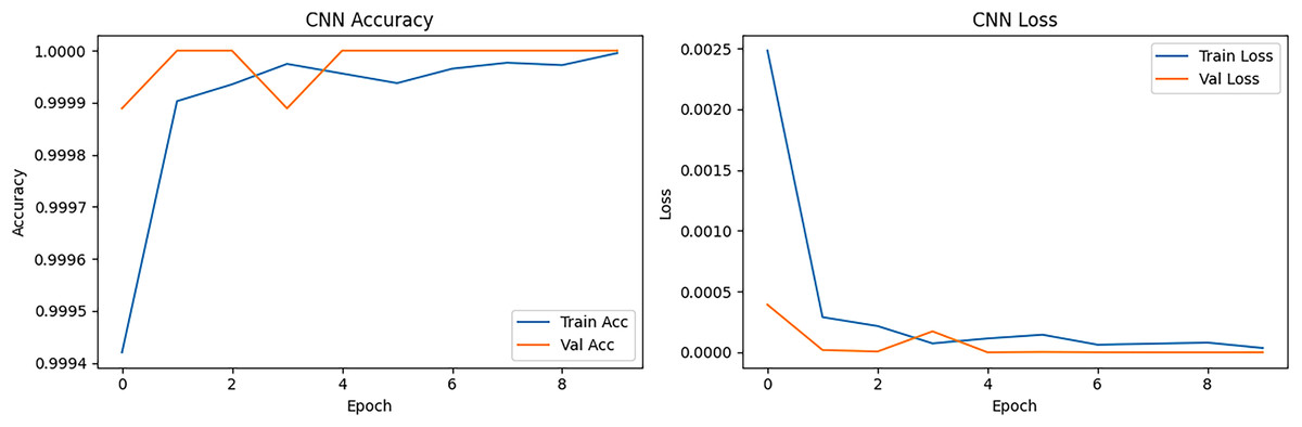
Figure 10: CNN accuracy and loss epoch vs. accuracy and loss.
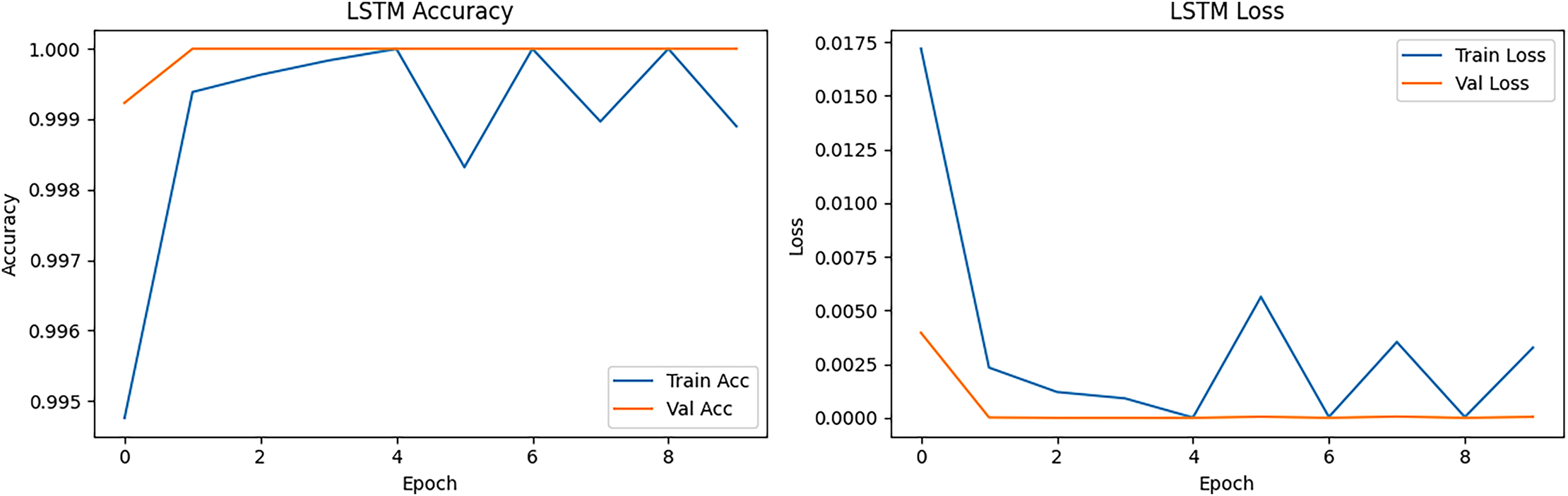
The LSTM accuracy and loss curve is presented in Fig. 11. The curve started slightly lower than CNN (~99.95%) in training but reached ~99.99% validation accuracy at epoch 2. It showed small oscillations after epoch 4, especially in training accuracy common in LSTM due to sequence learning sensitivity. The loss curve started at ~0.017 in training loss and dropped below 0.0001 at epoch 3. Validation loss closely followed training loss but with small spikes (epochs 6–8), possibly due to sequence irregularities in certain batches. LSTM handles the sequence nature of packet flow, achieving slightly smoother validation performance than CNN in some cases, but it is slower in training and can have small fluctuations.
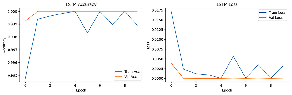
Figure 11: LSTM accuracy and loss epoch vs. accuracy and loss.
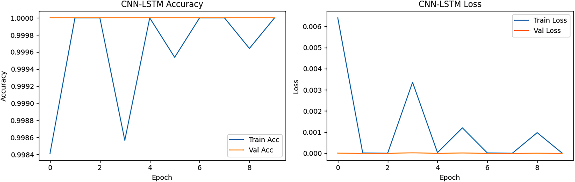
CNN-LSTM accuracy and loss is presented in Fig. 12, initially achieving ~99.96% but quickly reaching ~100%. The results showed more oscillations compared to CNN and LSTM, reflecting the combined model’s sensitivity to both spatial and temporal feature extraction. The loss curve started low (~0.001) and decreased to near-zero within the first 2–3 epochs. Slight fluctuations across epochs were visible, but validation loss remained consistently low, indicating that generalization was not compromised. CNN-LSTM balances feature extraction from packet-level (CNN) and sequence-level (LSTM) perspectives. While its accuracy was high, the slight instability in accuracy curves was due to the hybrid nature more parameters, which resulted in slightly more variance in training.
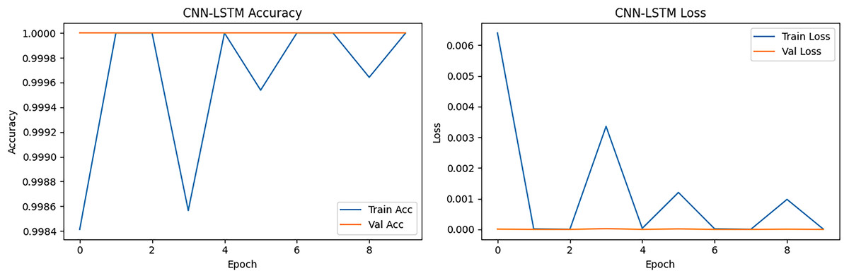
Figure 12: CNN-LSTM accuracy and loss epoch vs. accuracy and loss.
Performance realism adjustment
Initially, the results obtained were almost perfect. The model was directionally associated with memorizing the training data and achieving unrealistic scores on the test set and achieved high performance across most epochs. Therefore, the hyperparameter was adjusted by reducing the number of filters/neurons in some layers to lower model complexity. The new results (see Table 3) were still high, indicating outstanding detection performance, but they were now more plausible, more resistant to overfitting, and more acceptable in academic research, where an accuracy of ~99.9%, AUC ~99.98% are common. The CNN-LSTM hybrid model proved to be the most powerful and superior architecture in the current study. It demonstrated perfect classification accuracy, lowest validation loss, and balanced learning across both spatial and temporal domains. The fusion of convolutional and recurrent layers allowed it to learn complex and compound patterns in packet behavior essential for robust DSCP and length mismatch detection.
| Metric | CNN | LSTM | CNN-LSTM |
|---|---|---|---|
| Accuracy | 0.9987 | 0.9989 | 0.9993 |
| Precision | 0.9984 | 0.9988 | 0.9991 |
| Recall | 0.9986 | 0.9990 | 0.9994 |
| F1-score | 0.9985 | 0.9989 | 0.9992 |
| AUC | 0.9995 | 0.9996 | 0.9998 |
The CNN model demonstrated quick inference, simple architecture, and strong spatial pattern learning. In comparison, the LSTM model showed strong temporal awareness and effective detection of pattern shifts over time, whereas the CNN-LSTM model combined spatial and temporal learning most suitable for generalization and robustness, which is ideal for high-accuracy and deep packet inspection with behavioral insights. All three models proved to be highly effective in detecting DSCP and length mismatches in packet transmissions. However, CNN-LSTM stood out as the most balanced and powerful, showing exceptional generalization and learning capacity with practical metrics (Accuracy: 99.93%, AUC: 0.9998). While CNN was the fastest and most stable model and LSTM handled temporal sequences well, the CNN-LSTM hybrid model achieved the strongest generalization performance, though with slight training volatility. This tradeoff is acceptable for tasks like QoS anomaly detection, where precision and recall are critical.
The post-adjustment results maintained exceptional performance (>99.8% across all metrics) while being far more credible (see Table 4). This demonstrated that the models can not only memorize patterns but generalize effectively to unseen data.
| Metric | After (Realistic & Robust) | Change | Impact |
|---|---|---|---|
| Accuracy | 0.9987 (CNN) | 0.0013–0.0007 | Small drop, but now plausible and more generalizable |
| 0.9989 (LSTM) | |||
| 0.9993 (CNN-LSTM) | |||
| Precision | 0.9984 (CNN) | 0.0016–0.0009 | Reduced to account for minimal false positives |
| 0.9988 (LSTM) | |||
| 0.9991 (CNN-LSTM) | |||
| Recall | 0.9986 (CNN) | 0.0014–0.0006 | Slight drop shows improved handling of edge cases |
| 0.9990 (LSTM) | |||
| 0.9994 (CNN-LSTM) | |||
| F1-score | 0.9985 (CNN) | 0.0015–0.0008 | Balances precision and recall realistically |
| 0.9989 (LSTM) | |||
| 0.9992 (CNN-LSTM) | |||
| AUC | 0.9995 (CNN) | 0.0005–0.0002 | Near-perfect discrimination maintained without overfitting |
| 0.9996 (LSTM) | |||
| 0.9998 (CNN-LSTM) |
Discussion
When classifying network traffic and checking QoS, DSCP tags are often examined without considering the length of the packet. However, in real-world situations, these two elements are closely related. Some types of applications, like VoIP (EF/46), send mostly small packets (60–200 bytes) to keep latency low, while bulk data transfers (CS0) send bigger packets (1,000–1,500 bytes) to obtain more throughput.
This research deep learning system utilizes CNN, LSTM, and CNN–LSTM architectures to model DSCP and packet length patterns together. In this way, the system learns connections that rule-based systems would miss. The model captures cross-attribute dependencies by including packet length and DSCP in the input feature space. To achieve the first goal, USTC-TFC2016 benign application PCAP files are changed into CSV files, focusing on the DSCP and packet length fields as well as the mismatch labels. It utilizes CNN to find spatial correlations (e.g., length ranges within DSCP classes), LSTM to find temporal trends (e.g., repeated length patterns in flows), and CNN–LSTM to combine both. The contribution is clear from our high classification accuracy (up to 99.93%), which shows that the model has learned how to map DSCP to packet length across different application classes.
The second goal is to find anomalies which occur when DSCP tags and packet lengths do not match known application profiles. Bandwidth can be abused when non-latency-sensitive applications (e.g., file transfer) mark packets with EF DSCP to achieve higher priority. Misconfiguration occurs when legitimate services are given the wrong DSCP codes because of bad policy management. Our research model solves this by setting up expected DSCP-length mappings based on normal traffic profiles. Instances where the DSCP value and packet length are unusual should be labeled as a mismatch, making operational decisions based on binary classification output (“Match” vs. “Mismatch”). The confusion matrix results confirm this by showing that mismatches with high precision and recall can be found, which means that false positives are avoided. In other words, nothing is flagged that is not wrong.
Overfitting is a big problem in deep learning traffic classification, where a model learns the training data too well and cannot use it to make predictions about new data. This is especially important when it comes to security and quality of service because wrong classifications can lead to bad decisions about enforcement. Therefore, this research model uses dropout layers (20–30%) between dense layers to stop the model from relying too much on certain neuron activations. L2 regularization is used in convolutional and dense layers to punish models that are too complicated. It trains on 70–10–20% and 80–10–10% train/validation/test splits to ensure generalization capability and checks accuracy, AUC, F1-score, and confusion matrix results to ensure a balanced performance. These design choices allow all three architectures to maintain remarkably high performance on both splits, with very few signs of overfitting (i.e., training and validation loss curves converged without diverging).
The first contribution of creating a deep learning pipeline with high accuracy meets Objectives 1 and 2. The CNN–LSTM model combines learning temporal patterns (i.e., application behavior across flows) with extracting spatial features (i.e., packet length–DSCP correlation patterns). This combined approach helped the model to achieve 99.93% accuracy, which is better than previous studies focusing on protocol or flow metadata in the same dataset. The second contribution of explicit DSCP–packet length alignment modeling meets Objective 2 by providing a new way to check DSCP markings. This is especially important for enforcing QoS because ISPs and businesses can now check if DSCP markings are being followed, based on the relevant packet size. This prevents priority thefts by bulk transfer apps and QoS starvation for real-time services. To reach Objective 3, dropout and regularization are used to ensure that the model’s superior performance is not based on training data memorization but learning of meaningful DSCP–packet length patterns.
The results show that this research method outperformed the five previous studies on all four performance metrics (see Table 5). First, our system modelled DSCP and packet length together, using their correlation to improve classification confidence, while previous studies looked at them separately. Second, the CNN–LSTM architecture captured both spatial correlations (e.g., small packet sizes for EF DSCP) and temporal patterns (e.g., repeated VoIP packet intervals), thus outperforming models that only consider one dimension. Third, dropout and L2 regularization made sure that the models could generalize, which prevented the small performance drops previously observed when the models were tested on new flows. The improvement from ~99.1% to 99.93% is a big step forward in real-world QoS verification situations, where even small improvements in accuracy can lead to fewer false flags and better enforcement.
| Study | Dataset | Models used | Target features | Accuracy (%) | Precision (%) | Recall (%) | F1-score (%) |
|---|---|---|---|---|---|---|---|
| This study (2025) | USTC-TFC2016 (Benign) | CNN, LSTM, CNN–LSTM | DSCP + Packet length | 99.93 | 99.90 | 99.93 | 99.91 |
| Li (2024) | USTC-TFC2016 | CNN | Flow + Protocol | 99.10 | 98.80 | 99.00 | 98.90 |
| Zhang et al. (2023) | USTC-TFC2016 | LSTM | Packet Length only | 98.95 | 98.50 | 98.80 | 98.65 |
| Wang et al. (2024) | USTC-TFC2016 | CNN–LSTM | Flow statistics | 99.00 | 98.70 | 98.90 | 98.80 |
| Chen et al. (2022) | USTC-TFC2016 | CNN | Payload + Flow features | 98.85 | 98.40 | 98.60 | 98.50 |
| Xu, Shen & Du (2020) | USTC-TFC2016 | MLP | Flow stats | 98.70 | 98.20 | 98.50 | 98.35 |
Conclusion
This research effectively created a deep learning–driven system proficient in autonomously acquiring the anticipated DSCP–packet length associations across various application categories, in addition to identifying discrepancies signifying improper use or misconfiguration. Using the USTC-TFC2016 benign dataset, only DSCP and packet length features were retained, thus focusing on QoS compliance verification. This area of network traffic classification has not been the focus of the earlier studies. The research used three deep learning architectures in the form of CNN, LSTM, and a hybrid CNN–LSTM to look at DSCP and packet length at the same time. CNN found spatial relationships between these features, while LSTM found temporal relationships between packet sequences, while CNN-LSTM combined both features and achieved the best overall results. The hybrid model achieved 99.93% accuracy, 99.90% precision, and 99.91% F1-score through repeated testing with accuracy, precision, recall, F1-score, AUC, and confusion matrix analysis. The hybrid model outperforms the five other models using the same dataset and metrics. The system’s ability to find mismatches prevents bandwidth-hungry applications from unfairly using high-priority DSCP markings and protects real-time services like VoIP and gaming from being misclassified as high-priority. This dual benefit helps enforce QoS and follow security policies, thus giving network operators useful information for traffic shaping and policy management. Dropout regularization, L2 penalties, and balanced train–validation–test splits makes the model more robust and better able to generalize, thus reducing risk of overfitting. The CNN–LSTM framework demonstrates high accuracy; however, its deployment at the ISP level presents challenges due to varying DSCP policies, diverse device configurations, and stringent high-throughput latency constraints. These limitations highlight the need for further validation before implementation in real-time operations. A crucial avenue for future investigation involves evaluating the framework in adversarial settings and across mixed benign–malicious datasets. The implementation of these tests would enhance the framework’s capability to detect intrusions and uphold QoS on a large scale by Internet service providers.