
A reinforcement learning-based adaptive evaluation framework for personalized music education
- Published
- Accepted
- Received
- Academic Editor
- Siddhartha Bhattacharyya
- Subject Areas
- Human-Computer Interaction, Algorithms and Analysis of Algorithms, Artificial Intelligence, Computer Education, Neural Networks
- Keywords
- Music education, Adaptive teaching framework, Deep Q-Network (DQN), Task recommendation system, Personalized learning, Educational data mining
- Copyright
- © 2026 Li
- Licence
- This is an open access article distributed under the terms of the Creative Commons Attribution License, which permits unrestricted use, distribution, reproduction and adaptation in any medium and for any purpose provided that it is properly attributed. For attribution, the original author(s), title, publication source (PeerJ Computer Science) and either DOI or URL of the article must be cited.
- Cite this article
- 2026. A reinforcement learning-based adaptive evaluation framework for personalized music education. PeerJ Computer Science 12:e3464 https://doi.org/10.7717/peerj-cs.3464
Abstract
Evaluation of student performance in music education is recognized as a persistent challenge. The current methods of assessment, such as peer feedback, instructor observations, and rubric-based grading, are subjective and fail to deliver prompt and personalized feedback. Previous approaches have largely relied on static evaluation schemes like standardized grading rubrics and subjective instructor judgments like qualitative assessments without real-time feedback, but they failed to accommodate individual learning differences and dynamic adjustment of instructional strategies based on a student’s evolving abilities. To address these limitations, this study demonstrates a reinforcement learning-based adaptive evaluation framework designed for personalized music education. To optimize teaching interventions and customize learning experiences, the framework incorporates a task-selecting evaluation agent, a dynamic student model, and a continuous feedback mechanism. A Deep Q-Network (DQN) agent processes performance metrics like technical proficiency, expressiveness, sight-reading ability, and interpretative skills in real-time to suggest appropriate tasks and provide personalized feedback. A simulated dataset of students was used to train and test the model with different hyperparameters. These parameters are optimized through grid search and validation techniques. The results demonstrate that the proposed framework significantly outperforms baseline models, which include Q-learning, Proximal Policy Optimization (PPO), Soft Actor-Critic (SAC), Trust Region Policy Optimization (TRPO), Deep Deterministic Policy Gradient (DDPG), in terms of cumulative rewards, learning efficiency, and evaluation accuracy. Furthermore, the proposed framework exhibits superior adaptability by continuously updating student models and task recommendations based on ongoing performance data. This work offers a practical and scalable solution for personalized music education, contributing a step towards artificial intelligence (AI)-driven adaptive teaching systems in skill-based learning environments.
Introduction
The accurate and impartial evaluation in music education is recognized as fundamental features in fostering students’ mental, emotional, and creative growth. The process of learning music assists in development of technical skills and personal expression, emotional intelligence, and self-discipline (Yi, 2025). In formal learning environment like music conservatories, school music programs, and various online learning platforms, students may be evaluated in such a way that they receive self-paced, customized instruction and motivation (Ma & Wang, 2025). The subjective, inconsistent and dynamic nature of music makes its evaluation difficult and challenging. The use of available tools, frameworks and human instructors make use of automatic grading mechanisms. This result in one-size-fits-all assessments of students and ignore personal elements which are vital to performance and creative pathways (Wu, 2025). This type of generalize assessments failed to highlight the issues in learning music education and hinder learning (Coppi, 2024).
To tackle these issues and enhance evaluation accuracy and objectivity, numerous rule-based and computer-automated systems have been developed to improve the precision and impartiality of evaluations. However, attempts at basic automation have overlooked the importance of adapting to a learner’s individual progression and learning curve, greatly decreasing effectiveness (Sivamayil et al., 2023). In the more creative fields, particularly music, the inability to apply innovative perspectives also greatly stunted effectiveness. Difficult as it may be in personalized music education, the implementation of Virtual Reality (VR) and Augmented Reality (AR) technologies is groundbreaking. These technologies enable students to practice, perform, and receive feedback in real-time within an immersive supportive environment.
It employs the use of virtual spaces such as concert halls and rehearsal rooms, which are fully depicted in 3D. Learners can develop and practice performance skills in lifelike scenarios without having to leave the classroom or their homes. AR integrates virtual feedback or interactive visuals to the actual world through tablets, cell phones, and AR glasses. It can transmute students seeing fingers and rhythm cues to real-time over their instruments. Combining VR and AR with AI technologies and reinforcement learning frameworks such as Deep Q-Network (DQN) can provide real-time evaluation of performance data (pitch, rhythm, dynamics, and expression) and lesson content. Utilizing AI to enhance Virtual and Augmented Reality gives students the opportunity to fully control the lesson objectives and accomplish goals. This complete integration of VR and AR technologies with AI gives motivation, feedback, and engagement to the lesson while sharpening the skills discussed.
In the recent past, machine learning (ML) solutions have demonstrated potentials in the wider education scene as it can facilitate a custom content delivery and the modeling of learners (Abbes, Bennani & Maalel, 2024).
RL is a type of learning that evaluates teaching using continuous feedback, iterative updates, and accumulated experience. The cyclic and performative nature of music education aligns well with RL which make it a strong candidate for real-time, adaptive assessment (Sajja, Sermet & Demir, 2025).
The existing RL applications within the educational sector still seem to lack the focus needed to address the nuances involved with the forensic music assessment, technical precision, emotional expressiveness, and interpretive style. To bridge this gap, the current study focuses on creating a new RL method based on the DQN algorithm (Williams, van Ketel & Schaefer, 2023). DQN is chosen because it efficiently handles discrete action spaces and is more data-efficient than model-based RL. It offers stronger sequential decision-making capabilities than contextual bandits. The four action representing the dimensions of music education are Technical Execution (TE), Expressive Performance (EP), Sight-Reading Precision (SRP), and Creativity in Interpretation (CIT). These areas provides a balanced set of pedagogically meaningful adaptations. The system monitors fundamental characteristics of the student’s music performance (rhythm accuracy, sight-reading, timing and expressivity) and provides adaptive instructional feedback in real-time tailored to each individual student’s level of development (Kaur & Dogra, 2024). Using reward-penalty learning schemes, the model ensures that the likelihood of receiving feedback decreases as skill levels improve and become progressively indicative of mastery (Chen, 2024). This model fosters precision in assessment while supporting creativity, promoting motivation, and deeper engagement.
The proposed framework comprised of a multi-layered DQN model that tracks reward information in real time and make optimal instructional selections. To evaluate the learning pace of the students the study uses a dynamic student model, a task selection engine, and an adaptable feedback loop. Additionally, the framework integrates fundamental components of gamified learning environment which include tracking progress, issuing rewards for improvements, and personal goal setting to sustain motivation. In terms of performance the proposed model is compared with Deep Deterministic Policy Gradient (DDPG), Proximal Policy Optimization (PPO), Soft Actor-Critic (SAC), Trust Region Policy Optimization (TRPO), Reinforcement Learning (RL) models using various metrices. The results show that the proposed framework outperform all these variations in terms of feedback accuracy and learning efficiency alongside student satisfaction. This is in addition to the fact that as we are witnessing a shift of music education to digital and hybrid formats, combining this RL framework with virtual reality environments marks a development in the potential for immersive and interactive learning. The use of VR related technology make it possible to simulate realistic performance contexts for students which include ensemble and stage settings, and assess gesture, emotion, and spatial interaction in real-time. These features enrich the assessment component. Based on this motivation this research study is based by the central research question: Can a DQN-based agent improve the effectiveness of personalized evaluation and task recommendation in simulated music learning compared with standard RL baselines? To address this question, this study devise three different hypotheses. In first (H1), the DQN model is expected to achieve higher cumulative reward than Q-learning, PPO, SAC, TRPO, and DDPG under matched training budgets. Second (H2), the DQN model is presumed to have more stable learning results, which is indicated by a lower Reward Volatility Index and greater Engagement Stability Index. Third (H3), the DQN model will provide high degree of evaluation accuracy in various performance metrics when compared with baseline algorithms. These hypotheses form the basis for aligning the subsequent experimental results to measurable outcomes. The main contributions of this study are given as follows:
Explores the use of a DQN-based RL framework in music teaching for delivering adaptive, personalized feedback based on continuous performance evaluation.
Establishes a structured data collection protocol, which is used to capture core performance indicators and subjective learner responses.
Incorporates a penalty-based adjustment mechanism which enable the system to address performance deficiencies and adapt task difficulty levels responsively.
Demonstrates the effectiveness of DQN Model through comparative analysis with other reinforcement learning techniques in terms of optimizing instructional strategies, feedback precision, and overall learning outcomes in a simulated music education environment.
The remaining article is organized in the following way: ‘Literature Review’ discusses the related work on performance evaluation in music education and the application of reinforcement learning in teaching systems. ‘Reinforcement Learning and DQN in Educational Contexts’ present the motivation behind the proposed approach and highlights contributions, such as the use of DQN for adaptive feedback generation, real-time skill tracking, and personalized performance evaluation. It also explains how the proposed system performs better than other frameworks. ‘Proposed Framework’ details the design of the evaluation framework, describing the data collection process, DQN model architecture, training strategy, and feedback mechanism. ‘Experimental Results and Analysis’ outlines the experimental setup, participants, dataset generation, and result analysis. Finally, ‘Discussion and Analysis’ summarizes the study’s key findings, demonstrates the effectiveness of the proposed framework, and discusses its potential for future research and practical implementation.
Literature review
To ensure objectivity selection of different studies evaluated, this research work adopted a structured literature selection methodology. These works primary focus was on reinforcement learning in music education, adaptive assessment, ML in teaching feedback, and DQN in educational frameworks. Research work with empirical studies, RL/ML-based educational models, and adaptive or personalized assessment techniques are included while theoretical-only discussions, and duplicate entries are excluded. This process makes the section both comprehensive and aligned with the research focus of personalized music teaching via reinforcement learning. Studies on music education have focused on various strategies used in implementing and evaluating models such as peer-assessment systems, traditional examinations, and rule-based evaluation techniques which are depicted below.
Traditional and technology-based assessment in music education
Before the emergence of ML, most institutes used conventional ways for determining students’ performances such as tests and peer assessments. It is always challenging to adapt these approaches to different learning environments and these approaches appear fairly subjective. Research work, presented in Babu et al. (2025) focuses on the way conventional strategies such as tests and peer feedback construct music education. Some of them realized that these strategies are often unfairly implemented and lack flexibility. The authors in Barrett (2023) stated that the traditional tests often fail to assess a learner creativity and intellectual intelligence. Their observations emphasize the fact that peer reviews may be influenced by the nature and character of the reviewer a fact supported by work presented in Sofianos et al. (2025). They noticed that the general impression given would depend on the kind of reviewer involved, their experiences with the specific student included or encountered. Because of these demerits, researchers started interest in using other means of evaluating music teaching and learning.
Advanced technologies have given rise to new intelligent applications. For instance, work in Yue & Shen (2024) successfully conducted a study to unearth the possibility of using technology in music classes. Some examples of the technological advancements are enhanced learning equipment’s, which include digital software in learning. For example, software used to introduce learners to music notation aid the learners to develop their reading and writing skills. Same to audio tools, who can be used to give feedback on music pieces in specific manner. In another study (Förster, 2023), the authors explored how the use of interactive music applications can assist students in understanding music theory. In addition, Yang (2024) pointed out that the use of these gizmos can make lessons more engaging, they often fail to address emerging class peculiarities that are germane to male learners, and that compromises their utility.
Machine learning in music education
Applying such approach as ML models and methods is very helpful in making the evaluation of education more efficient as well as strategy planning. The work presented in Shuo & Ming (2022) noted that many authors have discussed the application of ML in music education studies. Others can look for patterns in large quantities of data. There has been a situation where researchers have adopted ML to make determinations on the performance of the students. Similarly, Latif et al. (2023) have also studied the application of ML for verifying accuracy of pits and timing during performativity processes. This enables factual evaluations and shows what has to be upgraded. But they overlooked prescribing specific techniques to be used when teaching the students. The authors in Yu et al. (2023) employed ML to predict how a student’s performance might evolve in the future. Still, the models are not capable of producing specific recommendations for each of the learners. Till now, all the methods for assessing and selecting the optimal approaches, RL is considered one of the most suitable methods applicable to research on education. While, research in Tang & Zhang (2022) explained that RL has been used in various contexts of education so as to help students achieve learning level 2.0 in language learning. In the same way, study in Cruz & Igarashi (2020) demonstrated that RL could control the intensity of educative games depending on how the students were performing. As such, these studies point that RL can increase engagement and the overall results of students.
Reinforcement learning and DQN in educational contexts
While the use of RL in a learning context has been a focus in the last 10 years, there is not much literature on its application regarding music education. Research work in Wu et al. (2022) investigated the DQN algorithm which integrates Q learning and deep neural network research. This approach enables one to define specific tasks with computable predictions. It has proven that DQN has the capability to learn well in environments that are not fixed. Therefore, applying DQN in music education could help analyze performance data to suggest better teaching approaches. Similar to RL, there are studies that focuses on adaptive learning systems in music education. The research work in Burak & Gultekin (2024) provide real time assessment and feedback about students by using an innovative adaptive scheme for schooling piano skills. It select suitable exercise levels based on each student’s progress. Although this method showed good results, it relied on fixed and predetermined rules. Likewise, study in Ng, Ng & Chu (2022) developed a guitar teaching system using set rules to customize lessons and make it dynamic. The issue with this method is that it lacks the adaptability and learning potential found in RL techniques.
Moreover, several studies confirm that gamification can enhance student motivation in music learning. For instance, work at Liu & Shao (2024) observed a 28% rise in student login frequency in a digital music learning app when badges and level progression were implemented. Similarly, Zhao, Narikbayeva & Wu (2024) reported that students using a gamified platform practiced 34% more minutes per week than those in a traditional classroom. However, such motivation spikes were temporary and tended to decline after six weeks without added novelty elements, indicating that long-term motivation may require progressive gamification layers or content refresh. Apart from the above, other studies examined adaptive systems that relied on fixed metrics and feedback loops. Their work showcased the early advantages of adaptive learning systems but identify the limitations regarding their elasticity and long-term usefulness.
Discussion and research gap
The research efforts described in this section have indeed brought a difference on music education by translating different approaches to assess as well as to include technology. However, most traditional forms of performance assessment are still prevalent, which rarely provide true measurement accuracy and are not adapted to the child’s needs. Technology and particularly the ML has made the assessments to be much more effective as well as fair compared to the traditional ways of assessment. Nevertheless, these methods can often be devoid of the individual approach to the child which is very important when teaching. On the other hand, especially by employing the DQN reinforcement learning techniques people are known to have developed interest and success in other areas of learning as well. However, there is still a gap when it comes to implementing the ML approaches directly to music learning. Thus, this study aims to fill that gap by developing a new assessment model that is informed by DQN to come up with better developed approaches towards the challenges and requirements encountered in pro music instruction.
Proposed framework
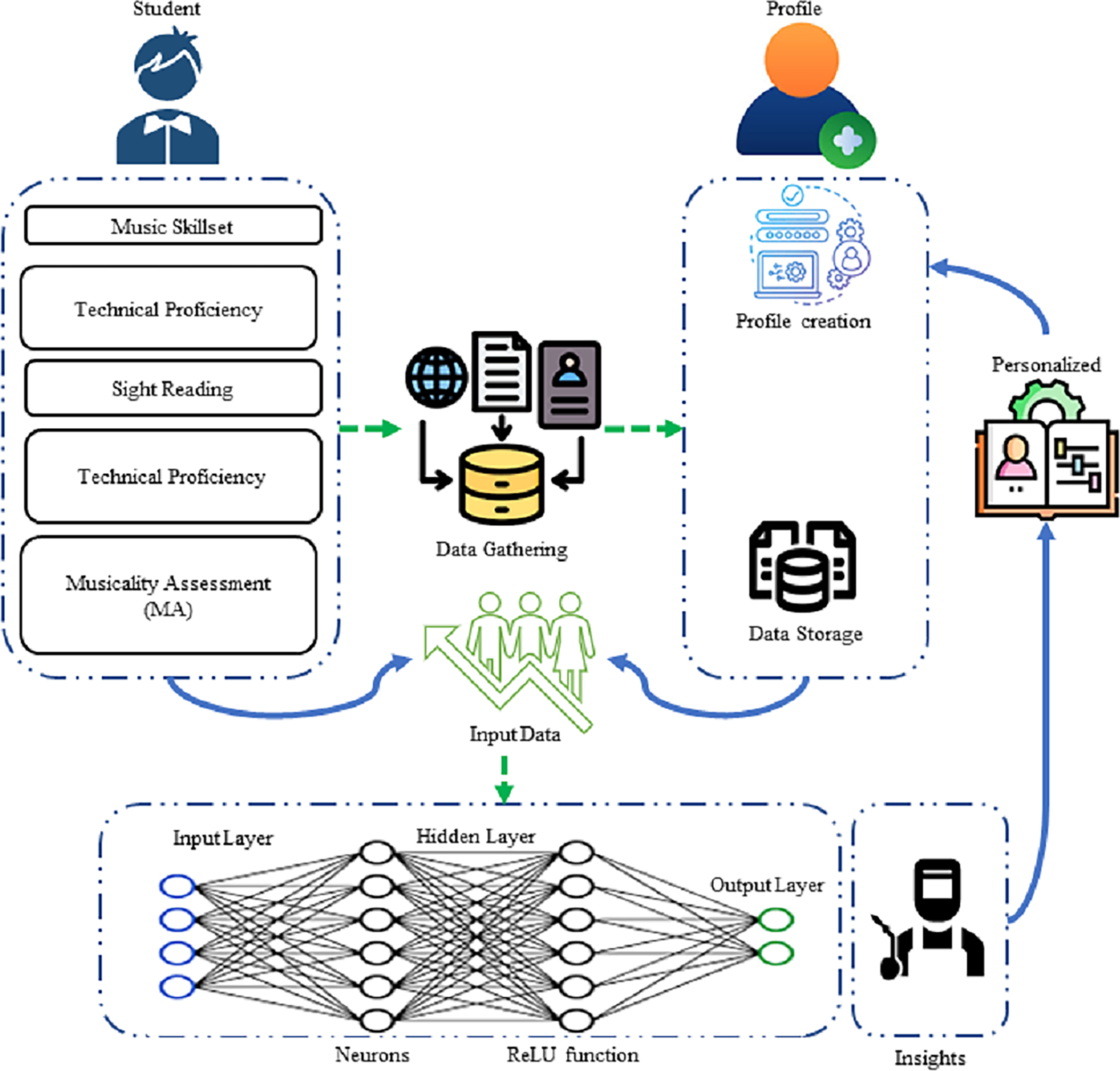
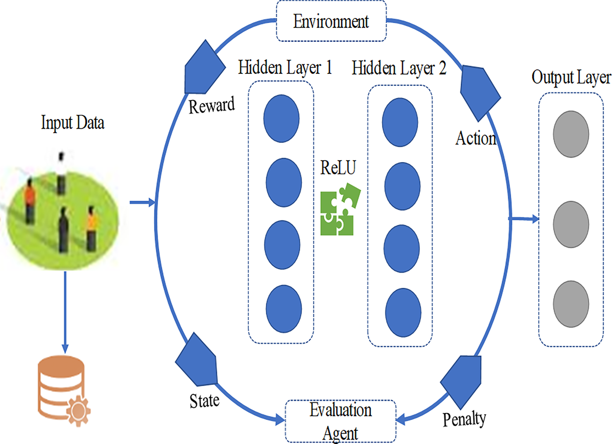
The framework for the evaluation of music teaching has two key parts: the system architecture and DQN analysis, System architecture describes major components of the model and DQN analysis refers to the use of a reinforcement learning model that maps student performance metrics to optimal instructional actions using Q-value estimation. These components combine to produce an adaptive and customized evaluation experienced framework. These sections describe the connection and interaction between the four major components of the study which are student model, evaluation agent, feedback system and data storage. The DQN analysis examines the way the algorithm contributes to better decision-making of the evaluation agent. This combination approach ensures specific and accurate evaluations. Figure 1 also shows different components of the proposed model including how the data about students is collected through the system architecture which also determines the right students based on their skills and behaviors. There is a feedback mechanism that gathers the opinions of students towards critical assessment items. The whole data is stored in a storage unit.
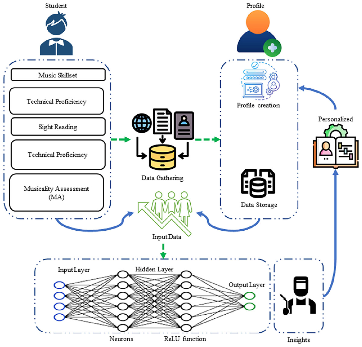
Figure 1: Workflow and modules of the proposed framework.
The proposed framework comprises several key components: data collection mechanisms, a projected neural network for data processing, the study’s penalty model, and reinforcement learning algorithms. Collectively, these elements establish a comprehensive, student-centered evaluation system that can be flexibly adapted to individual learning needs.
To make the evaluation process more concrete, the adaptive evaluation problem is modelled as a Markov Decision Process (MDP), defined as M = S, A, P, R, γ . The state space S captures learner attributes, the action space aaA encodes pedagogical interventions, the transition function P models change in learner performance under different actions, the reward function R evaluates learning progress and engagement, and γ is the discount factor. This specification provides the formal backbone for the proposed framework for ensuring consistency. For clarity and consistency, the symbols, parameters, and evaluation metrics employed in this study are summarized in Table 1. This notation is used uniformly throughout equations, algorithms, and figures.
| Symbol/Term | Definition |
|---|---|
| TP | Task Proficiency (0–100), student’s technical performance score |
| ME | Motivation and Engagement (0–100) |
| SR | Skill Retention (0–100) |
| IS | Instructional Satisfaction (0–100) |
| LP | Learning Pace, rate of progress per episode |
| P | Student preference profile (feedback/practice) |
| S | State vector = [TP, ME, SR, IS, LP, P] |
| A | Action set = {TE, EP, SRP, CIT} |
| TE | Technical Exercise |
| EP | Expressive Practice |
| SRP | Skill Retention Practice |
| CIT | Critical Item Training |
| R | Reward function: improvement in skills and learning pace |
| p | Penalty term for performance decline |
| γ | Discount factor (future reward weighting) |
| α | Learning rate |
| ε | Exploration rate in ε-greedy policy |
| ΔS | Change in average skill score |
| ΔLP | Change in learning pace |
| Tempo control | Derived from SR (rhythmic stability); smoothed over 5 episodes |
| Expressiveness | Weighted improvement in ME and IS scores |
| Accuracy | Weighted combination of TP and SR (normalized 0–1) |
System architecture
The system design of the proposed framework constitutes of four main components namely the student profile, assessment tool, response system and the information hub. These components are different in nature and functions but coordinate each other, in a synchronized and efficient way. Initially, the student profile collects significant information concerning the learners to the evaluation instrument. Then this information is used by assessment tool to choose relevant activities and provide the feedback which is used by the response system designed to facilitate the student. Lastly, all the significant information is tracked through its information hub in an adjustable method. The assessment tool also modifies as the students learn and develop. The student profile updates to mirror the learner’s growth. This ongoing process helps keep the assessment personalized and relevant. The model simulates 50 diverse learner profiles such that they are categorized on basis of their abilities. It consists of different proficiency levels which include beginner, intermediate, advanced. The dataset consists of various types of attributes that are related to variability in skill progression, feedback sensitivity, and task responsiveness. Empirical distributions of such attributes derived from real music education literature determine this simulation study. The proposed Evaluation Agent component, which is built on the DQN framework, interacts-communicates with this student model in order to choose contextually relevant instructional tasks and generate individual feedback. This architecture ensures that the complete process of the learning loop-from observation and state update to action selection and performance reinforcement-can be closed, scalable, and adaptable within a diversity of educational settings.
Architecture of student model
The student model is key module of the proposed evaluation system. It creates a clear and evolving picture of every student’s strength and learning styles. It helps in exploring different features of the student’s foundational musical abilities. Let consider S be a vector that includes various traits of students learning and indicates the current condition of the student model. Equation (1) present the state vector S in mathematical form:
(1) where each shows detailed attribute of the musical capabilities used for monitoring students performance. Each factor has a set range that assists in identification of students skills and progress over time. Table 2 provide details of these factors and their range.
| Characteristics | Description | Value range |
|---|---|---|
| Technical proficiency (TP) | Precision and accuracy in singing notes | 0–100 |
| Musicality (MI) | Emotional delivery and expressiveness | 0–100 |
| Sight-reading (SR) | Reading aptitude and learn music speedily | 0–100 |
| Interpretative skills (IS) | Personal interpretation and creativity | 0–100 |
In this study, the comprehensive performance of students in a music education program was evaluated by focusing on four key dimensions. The first dimension is technical proficiency (TP), which measures a student’s ability to execute notes, passages, and musical phrases accurately and without technical errors (Arnold, Bagg & Harvey, 2024). The second is musical expressiveness (ME), which evaluates the expressiveness, dynamics, and textural depth in a student’s performance. It is based on previous works identifying expressive communication as one of the most essential elements of the musical skill (Yang & Lerch, 2020). The third dimension is sight-reading (SR) which measures the ability of a student to execute a piece of music that he has never before practiced a skill that has been recognized as important in music curriculum (Que et al., 2023). The fourth and the last dimension is the interpretative skills (IS) which measures the skill of a student who ascertains the capacity of adding personal emotion, character and stylistic interpretation in a musical production (Reybrouck & Schiavio, 2024). As a whole, these measures make a balanced picture of the student proficiencies and measured general human progress in music studies. In particular, TP measures pitch accuracy of the student on the score producing performance. A performance scale from 0 to 100 is used, with 0 denoting very poor accuracy and 100 representing faultless technical execution. This indicator especially comes in handy during the assessment of a student to determine how prepared they are to work on compositions that are technically demanding. To give TP a highly-developed overview, a variety of performance measures are observed: accurate pitch, the measure of how many correct notes are played; hand posture and finger technique, the determination of how appropriate and efficient the hand location is and how the fingers are played, tempo consistency, it is checked whether the student has kept the appropriate and constant tempo throughout the performance or not and the dynamics control which shows the evaluation of how the student is able to balance the volume levels and sound clarity at various dynamic instruments. The various elements are all used to determine the resulting TP score which is mathematically determined as in Eq. (2).
(2)
ME measures the capability of the student to communicate and demonstrate emotion using his/her music task. The value of the scoring scale can be between 0 and 100 though a performance of 0 means there is no expressiveness in the play at all and a mark of 100 means a very expressive show that is touching to the heart. This attribute is essential in the evaluation of the ways in which students express the emotion and their artistic intentions via music. The four essential elements that are investigated to gain the ME score are emotional expression, meaning how well the performer manages to communicate with the feeling and mood; phrasing that measures the success of the student in making musical lines coherent and expressive; dynamic variation, which measures how effectively the student can apply the changes in volume and intensity and shape the performance; and articulation, which measures the clarity, sharpness, and precision of the initiation and release of notes. These subcomponents are edited together so as to get the final score of the E, which is shown in the Eq. (3).
(3)
SR is a score which determines a student ability to perform and interpret new music efficiently and within a brief time. This is measured in a scale of 0 to 100 with a 0 score representing extreme poor ability in sight-reading whereas a 100 score represents exceptional ability in sight-reading. This skill is critical towards the assessment of the level of preparation of a student to be able to deal with new and difficult compositions without rehearsal. This metric is determined by several criteria together: note accuracy, an evaluation of the accuracy of the notes being played; rhythm accuracy, an examination of the skills of the student at reading and performing rhythms accurately; tempo, a measurement of the skill by the student to maintain the steady and appropriate tempo during sight-reading; and fluency, a global reflection of the smoothness, continuity, and seemingly natural flow of the performance. A combination of these components gives the obtained final SR score by the following Eq. (4).
(4)
IS measure the ability of a student to convey creativity and self-interpretation in a piece of music. The scores are measured between 0 and 100 where 0 means there is no personal interpretation, and 100 means very creative, original, and expressive approach. The indicator shows the ability of a student to incorporate his/her personal style and musical identity into his/her performance well. This attribute is evaluated using several key indicators. First indicator is creativity, which is used to assess the imaginative use of phrasing, dynamics, and tempo control. Second one is originality, which measures the performer’s unique personal touch. Third one is emotional connection, which captures the depth of the student’s emotional involvement with the piece. Last one is audience engagement, which is used to evaluate the effectiveness of performer captivates and maintains the attention of the audience throughout the performance. These sub-indicators collectively contribute to the final IS score, as mathematically expressed in Eq. (5) below.
(5)
The average skill set of students selected in this study is calculated using the following equation.
(6) where TP shows the technical proficiency, ME denotes musical expressiveness, SR is sight-reading and IS is interpretive skills. The availability of updated data in student model enable the evaluation agent to generate up-to-date insights. To ensure that student model is on track, a few important aspects are examined, updated and adjusted regularly. These aspects cover the student’s ability in various musical areas which include speed of learning, and their preferences for receiving feedback and practice activities. For every evaluation task, the model provides clear stats like accuracy, tempo control speed, expressiveness, and evolution of students performance over time. Shared data features present a more detailed view of areas where the student shines and where they struggle. The learning pace (LP) of a student’s performance is calculated using Eq. (7) described below.
(7) where denote the value of average skill metric at a certain time . shows the time value of past former assessment. It describe how effectively the student is improving in a specific skill. Likewise, to inspect long-term performance of the proposed method this algorithm makes use of a moving average as showed below in Eq. (8).
(8) where S(t) represent the skill metric calculated at certain time t and W denotes the Window size used for moving average. Moreover, it also shows how many previous evaluations are considered. This method has the capability to reduce the issue of short-lived fluctuations and highlights improvements in daily efficiency. The approach uses both past and live data to maintain an accurate picture of how students are learning a specific music skill. Whenever a learner completes an assessment, a value is recorded against each attribute of the profile. This includes the precise number of grades received along with more subjective insights, like how well the task was presented. This is key feature of the system because it has capability to integrate both numerical and descriptive data to assess the learner’s performance. To estimate future skill metrics, this research utilize the linear regression method as shown below in Eq. (9).
(9) where represent the interrupt factor of the regression mark and is the slope of the regression line while X is the independent variable e.g., time, effort, or another factor affecting Y. The student proposed model uses a personalized learning method that adapts to individual growth. This approach tracks how a student’s skills change as they engage with the material. For example, when a student excels in rhythm exercises, the system will recognize and enhance that skill. On the other hand, if someone has difficulty with finger placements, the system will indicate that extra attention is needed there. This responsive feature helps keep assessments relevant to the student’s abilities and development path. The mathematical representation of this concept is listed below in Eq. (10).
(10) where shows the present learning rate. Illustrates the updated learning rate. LP indicates the learning pace, while MaxLP indicates the maximum learning bound recorded. In addition to these factors, what the students prefer and how students have preferred to learn have also been taken into consideration by the model. Two students may benefit from specific analysis of micro aspects of their play whereas another student may benefit more from general remarks on musicality. The model keeps record of these preferences in order to provide feedback on what is most effective for each type of learner. The skills in this research cover teaching performance based on various teaching approaches. For beginners, the skill thresholds are set at . For and for advanced skills it is defined as . These milestones are essential for locating the particular abilities of a student, as well as the organizing of evaluation tasks. This model very accurately monitors measures of each of the assessment tasks. The data set for the current work is generated through the use of artificial student records for music learning in education. It also comprises such artificial records that reveal different sides of musical performance. The participants included 50 simulated students from a music academy ranging from first time learners and learners with considerable experience. The evaluation was done for a period of 6 months and at the beginning and at the end of each month. This resulted in seven different types of assessment points and the initial assessment alone. Data was gathered on four primary skill metrics during each assessment: TP, ME, SR and IS with values from 0 to 100. The other recorded parameters were each student’s LP, a record of average skill improvement over time, preferences for feedback, and practice tasks. From the data that was collected on each of the students, TP, ME, SR, and IS scores at each assessment period were recorded. Thus, the learning rate is calculated in between the consecutive evaluation points, in combination with the moving average skill indicators in order to analyze long-term tendencies. Specific measurement criteria for the tasks of evaluation were also recorded including accurate intonation, tempo control, expressive playing and improvement over time. This approach ensures one gets a balanced view of every student in terms of what he/she is good at or vice versa. For the purpose of monitoring and evaluation a tracking format is prepared for each student which shows the details of skill parameters and progress frequency. Table 3 described below shows sample tracking board for the dataset which has been used in this study.
| S.No | 1 | 2 | 3 | 4 | 5 | 6 | 7 | 8 |
|---|---|---|---|---|---|---|---|---|
| Attribute | Student-ID | Time period | Technical proficiency (TP) | Musicality assessment (MA) | Sight reading (SR) | Interpretive skills (IS) | Average skill metric (ASM) | Learning pace (LP) |
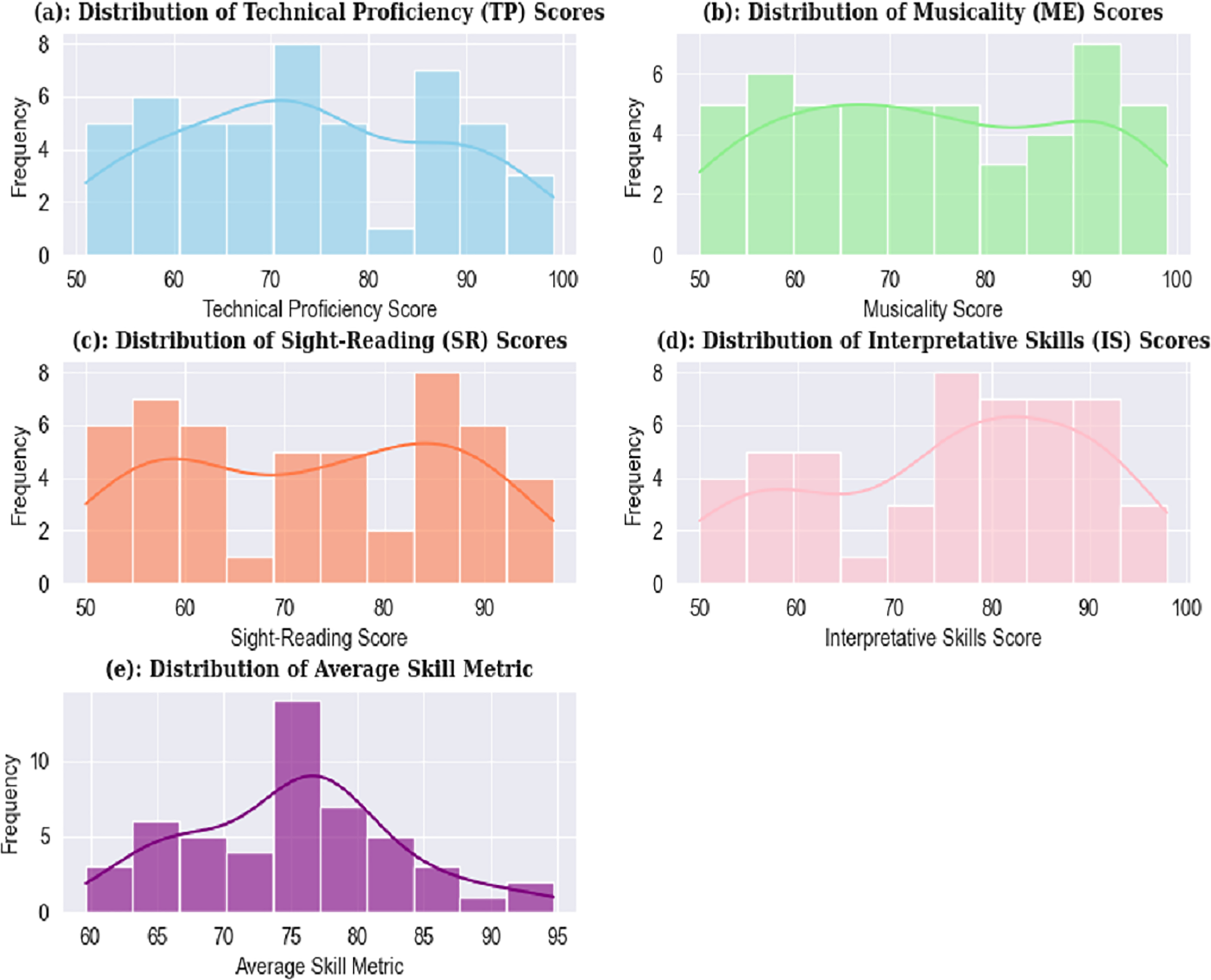
This table shows the performance of students in terms of comprehension and musical skills. It enable instructors to easily identify the students who need any additional support and address each student’s learning requirements. The method assess the students, and relevant data was collected in form of a dataset. Upon analyzing the dataset several performance distributions were observed, as illustrated in Fig. 2. The visualization shows that the distribution of TP scores is helpful in identification of prominent clusters of student performance levels. Similarly, the ME score distribution is used to captur variations in students’ expressiveness and engagement. The SR scores represent the time taken by students to accurately sight-read a new piece of music from start to finish. The IS score distribution reflects how creatively and personally students interpret and approach a musical piece. Lastly, the average skill metric combines TP, ME, SR, and IS scores and provide a comprehensive indicator of each student’s overall musical ability.

Figure 2: Distribution of records based on different music skills.
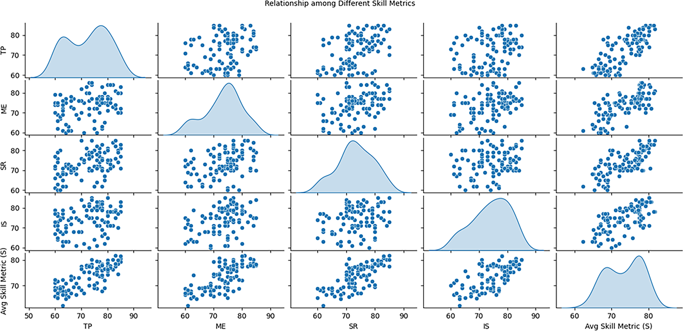
Similarly, it is clear from the assessment of different performance indicators described in Fig. 3, which demonstrate students’ strong and weak sides in different skills. It plots scatter plot for every possible combination of the metrics to show whether they are related e.g., technical proficiency and musicality. The diagonal sections also present Kernel Density Estimation (KDE) that provides an understanding of shape of each metric showing if the scores are normally distributed or not. This setup also gives a view of how different skills relating to the task interphase and the general distribution of each metric.
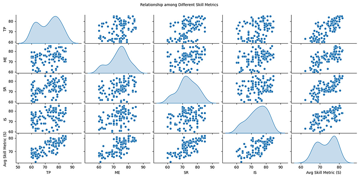
Figure 3: Relationship among different variables of students dataset.
Any data collected in the various phases is safely stored in a database. This is an information repository that includes what is derived from sources including practice, initial/feedback estimations and the like. Every record in the database is tagged with date stamp and associated with the student identification number. Due to structure, every student’s progress during different period is properly tracked and recorded in the repository. The data gathering procedure is mathematically represented or symbolically described in Eq. (11):
(11) where D(t) means the data collected at time t and R(t) represent the reward value or improvement score at a certain time t.
Evaluation agent
The assessment tool assists with the identification of the developments in a specific student’s musical performance and with facilitating practice with both interesting modes of interaction and multi-faceted instructional techniques. It draws on the assessments from early lessons and provides individualized feedback which allows learners adjust their approaches to studying in response to their results. The assessment tool is based on outcomes of the first evaluation. TP, ME, SR and IS scores are collected for each learner. An average of level of skill is calculated using an average skill value S given, by the following equation which was described above. This formula serves as a foundation for measuring how well students are doing. This tool is important for choosing strategies that enhances students’ abilities. These strategies include options like offering of targeted feedback, assigning practice activities, and altering instructional methods. The objective of each strategy is to reduce weaknesses highlighted in the skill metrics of learner. The strategy selection process can be mathematically illustrated in Eq. (12) given below:
(12) where A shows the chosen action, s denotes the current state, and Q(s, a) indicates the Q-value associated with action A in state S. There are four major parts that will be focused on in the practice session. Technical exercises (TE) will supplement the accuracy and precision of the pitch accuracy and precision by using scales, arpeggios, as well as technical studies. This shall result in an improved overall TP. Expressive playing (EP) is used to foster musicality by exploring the dynamics and phrasing music in form of different pieces. This will help elevate ME. The practice of Sight-reading (SRP) will strengthen sight-reading skills (SR) by regularly introducing new and increasingly challenging pieces. Lastly, creative interpretation tasks (CIT) will enhance IS which will inspire students to play with tempo, dynamics, and articulations. This will result in unique renditions of pieces. Various actions taken to elevate skill metrics and assess student learners are shown in Table 4.
| Action ID | Action type | Description | Skill |
|---|---|---|---|
| 1 | TE | Practice scales and arpeggios | TP |
| 2 | EP | Interpret a piece with varying dynamics | ME |
| 3 | SRP | Sight-read a new music piece | SR |
| 4 | CIT | Create a personal interpretation of a given piece | IS |
The evaluation agent gives feedback on the student’s performance based on chosen actions. If a student shows low TP, the agent may suggest focused practice on pitch accuracy. The feedback aims to help the student enhance particular skill metrics tailored to their needs. The effectiveness of this feedback is modeled as Eq. (13) below:
(13)
Here, R stands for the score received from the feedback. The agent changes its actions according to how students react. It modifies the Q-values to show how well the actions worked and assists in bettering choices down the line. The update formula for the Q-value is as follows in Eq. (14):
(14) where depicts the learning rate, represent the discount factor, S is the new state and a show the next action to be taken. The agent regularly checks how students are doing to track their progress. After giving feedback and practice tasks, it updates their skill metrics. These metrics include the new average skill score (S′). It also calculates the updated learning pace (LP′). The learning pace is gauged in Eq. (15) below:
(15) where t2 is the current time and t1 is the previous evaluation time. The new dataset contains information on the performance of students based on their skill use and the rate of learning of each student. With this new dataset, the learning model can now be improved on a regular basis. It enables the evaluation agent to adapt its strategies to improve the overall learning outcomes. Here, the student’s specific requirements are addressed whereby the evaluation agent provides personalized guidance on how to enhance their musical capabilities in relation to focused practice. In this case a student named Alex will be assumed. Say, for example, Alex indiscriminately assesses TPs = 70, MEs = 65, SRs = 75 and ISs = 60. Based on this graphic, one can estimate the average skill metric S using Eq. (16):
(16)
The numerical outcomes obtained from the study also suggest that Alex has the least IS score. An action is selected in order to enhance Alex’s interpretative abilities through a creative interpretation activity. After the action is determined to improve the IS of Alex, it is time to update the Q-value of an action. For this particular Q-value update the use of Eq. (14) is made. In selecting an action, the agent consider the Q-values of all possible actions with respect to state S and chooses the action that has the highest Q-value. Also, the agent provides Alex with some comments meant to encourage the semantic search and personal analysis. This feedback may require actions related to the expression of feelings, and effectiveness of this feedback is described as R. Stand on the equation updates it as per Eq. (17):
(17)
With a new plan in place to boost how well the technique works, it is time to refresh the Q-value. This update relies on closely tracking and evaluating the skills involved. Let us say the agent spots Alex’s latest scores: TP = 72, ME = 68, SR = 77, and IS = 68. From this, the new average skill metric S′ can be calculated as per Eq. (18) below.
(18)
The learning pace becomes as depicted in Eq. (19):
(19)
The agent then updates the Q-values which is built on Alex’s improvement as described in Eq. (20) given below.
(20)
The agent is used to check how Alex is performing at the next evaluation stage. It update the dataset and demonstrate future plans related to music education. In this way, Alex gets personalized support that fits their unique journey. The agent keeps is regularly monitoring Alex’s growth for the next 6 months. It updates skill metrics and adjusts how fast Alex learns to give better feedback and task suggestions. This flexible method enhances Alex’s learning experience and provide a well-rounded and tailored music education. Table 5 shows the new data for Alex.
| Student-ID | Technical proficiency | Musicality assessment | Sight-reading | Interpretive skills | Average skill metric (S) | Learning pace | Step |
|---|---|---|---|---|---|---|---|
| 1 | 70 | 65 | 75 | 60 | 67.50 | 0.0 | Preliminary |
| 1 | 72 | 68 | 77 | 68 | 71.26 | 3.76 | Mediation |
Algorithm 1 explains the working of evaluation agent. It uses an ML method to monitor and enhances student performance during a predefined evaluation timeframe. To start, it sets up Q-values for all likely actions of learner. These actions are performed for each student listed in the dataset. Next, it defines a average skill based on the performance metrics. In a learning loop, the algorithm continuously checks the current status of the student and select an action based on the Q-values. It perform the action and tracks the essential updates in the values. After getting the new values, it refreshes the state and reward, along with the Q-values and notes performed in the learning pace. This process continues until the evaluation period ended. The concluding results feature update student scores, learning pace, and improved Q-values. The evaluation agent algorithm starts by initializing Q-values for all possible state-action pairs. Initially, performance metrics of each student listed in the dataset are measured which consists of TP, MA, SR, and IS. The values of these metrices are retrieved from dataset and averaged to compute an initial skill score. During each evaluation cycle, the agent records the current state and selects a teaching action using an ε-greedy policy. It then applies that action on the learner. After observing the new state and reward, the values of skill metrics are updated and a new average skill score is computed. The learning pace is then calculated based on skill improvement over time. Q-values are then updated using the Q-learning rule which combine the immediate reward, discounted future rewards, and the previous Q-value. This loop continues for the set evaluation period, after which updated scores, learning paces, and final Q-values are recorded. The recorded values are then used to provide personalized, adaptive feedback for each student.
| Input: Init_Values, Eval_Period, Α, Γ |
| Output: Learning Pace, Updated_Scores, Q-Values |
| 1 Initialize Q-Values Q(S, A) State-Action Pairs |
| 2 While Each Scholar in : Init_Values: |
| 3 T1 = 0 |
| 4 Regain Primary values (ME, IS, SR, TP) |
| 5 Compute Original Average Skill S |
| 6 S = (ME +TP + SR + IS)/4 |
| 7 While Present Period < Eval_Period: |
| 8 Spot Up-to-Date State S |
| 9 S = (SR, IS, TP, ME) |
| 10 Choose Action A Utilizing Policy Π (E.G., Ε-Greedy) |
| 11 A = Argmax_A Q(S, A) |
| 12 Action Execution A And Feedback/Task |
| 13 New State S′ And Reward R |
| 14 Performance values (TP′, ME′, SR′, IS′) |
| 15 Estimate New Average Skill S′ S′ = (TP′ + ME′ + SR′ + IS′)/4 |
| 16 Gauge Learning Pace LP′ LP′ = (S’ − S)/(T2 − T1) |
| 17 T2 = Current_Time |
| 18 Apprise Q-Values |
| 19 Q(S, A) = Q(S, A) + Α * (R + Γ * Max_A′ Q(S′, A′) − Q(S, A)) |
| 20 Update S = S′ & T1 = T2 |
| 21 Record values |
| 22 End While |
| 23 do While() |
| 24 Output: Updated_Scores, Q-Values, Learning_Pace |
DQN algorithm for adaptive music teaching evaluation
The RL algorithm plays an important role in assessment of music teaching. It analyzes various types of data on how students perform during music classes. It also enable the evaluation agent to learn and adjust in real time. In this study, the DQN algorithm is utilized by merging Q-learning with deep learning methods. This will result in successful management of complex states and action spaces. The essential parts of this algorithm include the following:
Students state analysis
The term state is used to show how well each student perform in music class based on various assessment tools. For each student selected from the specific group of dataset, the state vector ‘s’ includes TP, ME, SR, and IS. Moreover, the state considers the student’s learning speed along with their preferred feedback and practice activities. Mathematical, the state vector can be defined as per Eq. (21) given below.
(21) where LP displays the learning pace and P describes the preferences.
Action space analysis
The action space A includes various activities that the evaluation agent can carry out with students, helping to improve its effectiveness. Each action plan explain specific goals designed to target particular skill metrics, such as TE, EP, SRP, and CIT. The objective of these actions is to boost different areas of the student’s performance. The action space A is illustrated as in Eq. (22):
(22)
Reward function
The reward function is used to track student’s performance and how it gets better after tackling specific tasks. It identify shifts in skill metrics and the overall rate of learning by students. This aim of this reward is to motivate behaviors that result in noticeable advancements in how well students do. The function R can be expressed as per Eq. (23):
(23) where portrays the alteration in the values of average skill metric, informs a weighting feature and denote the modification in the learning pace. If value of Alex’s TP progresses from 70 to 72 after a TE event and his average skill metric S expands from 67.5 to 71.25 the reward value will become as depicted in Eq. (24):
(24)
Penalty function
The penalty function plays a key role in the suggested model. It discourages activities that will negatively affect the learning of students. Basically, it assists in avoiding teaching systems that are ineffective and encourages decisions that will create better learning activities. The model is penalized whenever the performance of a student in any of the areas diminishes after a lesson. The penalty function, denoted as p and can be expressed mathematically as Eq. (25):
(25) where n represent the total number of attributes used for evaluating performance, is the weight value assigned to the ith attribute and Δsi denotes the negative alteration in the ith attribute’s score. The performance attributes depicted by si comprise MI, RC, TP expressiveness, IS and SR such that each scored from 0 to 100. The importance of each attribute is considered for the overall assessment. Imagine a situation where a student’s results in three key areas decline following a lesson. The attributes reflect changes as follows: Musicality = −3, Rhythm Consistency = −4 and TP = −5. Let us say the weights assigned to these attributes are: w1 = 1.5, w2 = 1.0, and w3 = 1.2. In this case, the penalty p can be determined as in Eqs. (26), (27), and (28):
(26)
(27)
(28)
In this context, the negative mark shows a cost. A larger negative number means the model faces a bigger cost for its choice. Throughout training, this cost is deducted from the reward to adjust the Q-values. This cost factor plays a role in figuring out the reward. The overall reward, which considers the cost, helps adjust the Q-values, steering the model towards better learning methods.
Q-value update analysis
The Q-value shows the expected total reward when taking action, A in state S. The DQN algorithm changes these Q-values using the rewards it observes and guesses about future rewards. It follows a specific update rule to adjust the Q-values as per Eq. (29):
(29) where shows the learning rate, depicts the discount factor, s′ represent the new value of state after execution of action a and a′ is the next action. Algorithm 2 is used to updating the Q-values.
| Initialization of Q-table with various initial values for all pairs of state-action |
| While state s in a set of S: |
| For action a in a set of A: |
| Q(s, a) ← New value |
| End For |
| End While |
| Define indicators |
| ε ← exploration rate γ ← discount factor α ← learning rate |
| For event = 1 to total_events: |
| s ← initial state |
| While s != End: |
| If random(0, 1) < ε: |
| a ← showing random action from A |
| Else: |
| a ← argmaxa Q(s, a) |
| r, s′ ← takeaction(a) |
| Qnew(s,a)=(1 − α) × Qold(s,a) + α × (R + γ × a′maxQ(s′,a′)) |
| s ← s′ |
| If s′ is end: |
| Break from loop |
| End While |
| End For |
The process begins off by creating a Q-table that contains values for every state-action pair, along with key settings like the discount factor (γ), learning rate (α), and exploration rate (ε). At the beginning of each episode, the algorithm starts from a set of initial state and picks actions according to a ε-greedy approach. This technique strikes a balance between trying new things and using known strategies. Once an action is taken, a specific reward follows. Receiving this reward or a penalty influences the next state. This feedback is used to adjust the Q values for the current state-action pair based on the reward received and the highest Q value from the new state, continuing until the process hits a terminal state, where values stabilize.
Proposed DQN algorithm
The proposed DQN algorithm uses a neural network that helps in estimation of the Q value. It select the action required for improving students skills. The neural network comprised of a state vector (s) as input. It then gives a Q-value for each action in the action space (A). The network has an input layer, three hidden layers and an output layer. In our implementation, the DQN follows established practices to ensure methodological rigor beyond tabular Q-learning. Specifically, an experience replay buffer of 50,000 transitions was used, with mini-batches of 64 sampled uniformly after a 1,000-step warm-up. A separate target network stabilized training, updated via hard copy every 1,000 steps (τ = 1.0), though soft updates (τ = 0.005) were also verified. The agent was trained using Adam (learning rate 1e−3, β1 = 0.9, β2 = 0.999) with a mean squared error (MSE) loss on the temporal-difference error and gradient clipping at norm 10.0. Exploration followed an ε-greedy schedule starting from ε0 = 1.0, decaying to εmin = 0.05 over 20,000 steps. Finally, the discount factor γ was set to 0.95 to reflect the importance of balancing immediate corrective feedback with long-term skill development in music education. These components collectively ensure that the model represents a full DQN framework, distinguishing it clearly from simplified Q-learning variants.
Input layer
The input layer of the proposed framework is composed of four neurons. Each neuron is used for an important measure of the student’s musical abilities. This layer is responsible for taking the input and creates a vector. This vector captures the student’s current skill metric. For example, Alex’s starting state looks like Eq. (30):
(30)
These values are used as the starting point for additional processing in the hidden layers. TP, ME, SR, and IS values are adjusted to make sure that all inputs are on the same scale. This step is important for the network to train more efficiently. Normalizing helps avoid any input overpowering the others because of its size. It usually scales the values to a range like [0, 1] or [−1, 1]. In our case, we apply min-max normalization to bring the inputs into the [0, 1] range. The min-max normalization formula as depicted in Eq. (31) is applied here:
(31)
In this equation x shows the actual value. is the least value of the indicator in the dataset. is the extreme value of the feature and is the standardized value. For instance, if the value of TP score fall in a range from 0 to 100 and Alex’s score is 70. The calculated normalized value for TP can be mathematically described as below in Eq. (32).
(32)
Applying this to all features, Alex’s normalized state vector becomes as in Eq. (33):
(33)
Hidden layer
The Q-value is estimated by the hidden layer in the suggested model. It becomes more efficient by tweaking the input and aiming for better convergence. There are two key types of hidden layers in this model. The first hidden layer has 64 neurons, and it make use of ReLU activation function, as shown below in Eq. (34).
(34)
This activation function adds a twist to the model, letting it pick up on patterns beyond just straight lines. Because there are 64 neurons in this layer, the network can grab most of the important traits and connections between various music skills. Here, the state vector is altered to more complex one by reshaping it. It emphasizes the important constituents that would be indispensable for the nesting layers. There has been a use of 64 neurons for the second hidden layer also, with ReLU as activation function. This layer goes even deeper into the features coming from the first concealed layer and makes them sharper. The second hidden layer provides additional measurements make it possible for the network to comprehend more complex relations among the constituent attributes. This layer, by obtaining the output from the first hidden layer, improves the network’s discrimination power in terms of student’s performance level thereby increasing the accuracy of Q-value prediction.
Output layer analysis
The output layer used by this study has four neurons. Each neuron of the hidden layer matches one possible action: TE, EP, SRP, or CIT. This layer’s output shows the Q-values for every action. These values depend on the current state and mathematically denoted using below Eq. (35).
(35)
The Q-values demonstrate the total probable future rewards measured for each action. They help the agent decide which action will lead to the most student improvement. For example, if the Q-value measured for TE is the highest, the agent will pick technical exercises as the next step. Architecture of the proposed model is described in Fig. 4.
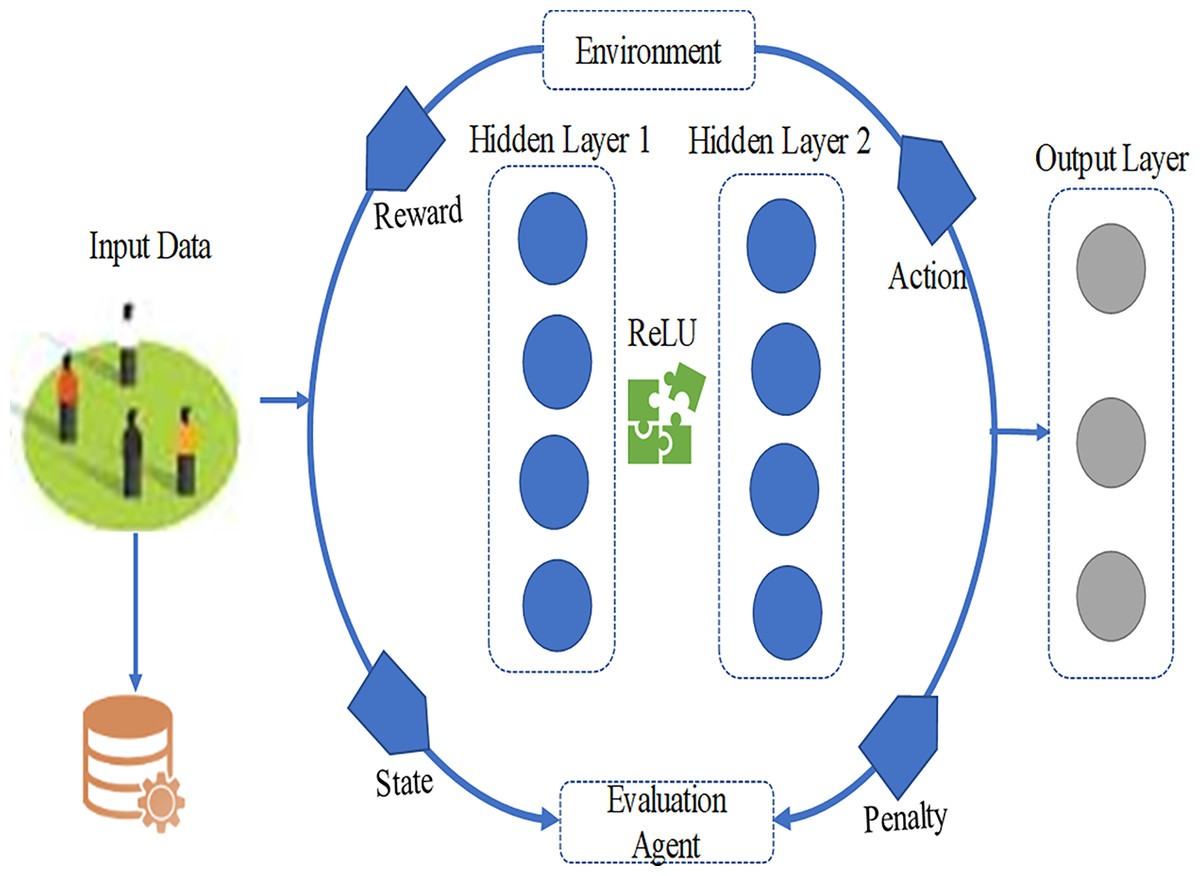
Figure 4: Architecture of the proposed DQN model.
Analysis of loss function
The loss function is used in the training process of the proposed model. It describes the MSE among the estimated Q-values and the target Q-values. The targeted Q-values are dependent on the perceived rewards along with the maximum Q-value for the next state as illustrated by the Bellman equation, which is described in Eq. (32). The training makes use of back-propagation method to plummet the loss function which is used to compute the variance between the forecasted Q-values and the target Q-values as in Eq. (36).
(36) where N present the total count of samples in the mini-batch, depicts the target Q-value and is the foreseen Q-value. This loss function makes sure that the network minimizes the difference that exists between the actual yielded values and predicted Q-values, with time increasing its accuracy of predictions. A network is fed a batch size of the state-action-reward-next state tuples. Using the new calculated error, the weights of our network are updated so that it works more in favour to minimizing overall loss. It optimizes the weights using stochastic gradient descent (SGD) or more advanced variants like Adam several important parameters significantly affect the training process while learning a neural network using DQN algorithm. These are the learning rate, discount factor, exploration decay rate, batch size and number of episodes. It is important to interpret these parameters for successful model training and convergence towards an optimal policy. Learning Rate (α) is use to handle the size of the stages implemented during the optimization process. This phase also update the weights of the network. Mathematically, if θ denotes the weights of the neural network and J(θ) shows the slope of the loss function J in terms of θ then the update instruction can be expressed as .
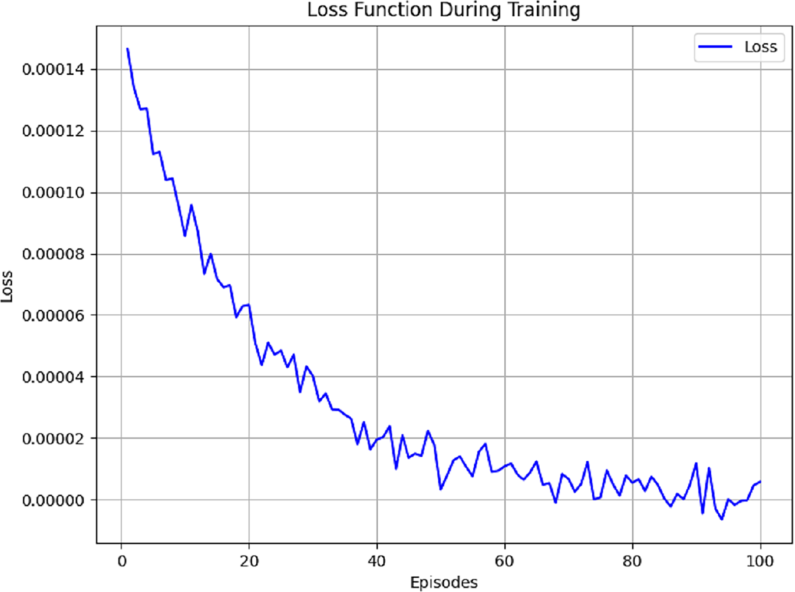
If the learning rate of the agent is selected too low, the model takes its time to learn and needs loads of iterations to reach a solution. This can lead to training sessions that drag on forever. On the flip side, a learning rate that’s too high might throw everything off balance. This can make the model jump over the ideal solution and end up going off track. A learning rate optimal for most deep learning applications is between 0.001 and 0.01. Considering the balance between efficiency and stability sought in this study, a learning rate of 0.001 is ideal. The Discount Factor (γ) is another important piece in the Q-learning discounting future rewards. It is between 0 and 1. If the model is learning, the loss function will trend down. Initially, loss is high due to random weight, the state-action space is being explored and there is unsupervised learning, but it will drop as the training progresses. This shows the model is improving its Q-value prediction and overall performance. The loss trend in Fig. 5 is for 100 episodes.
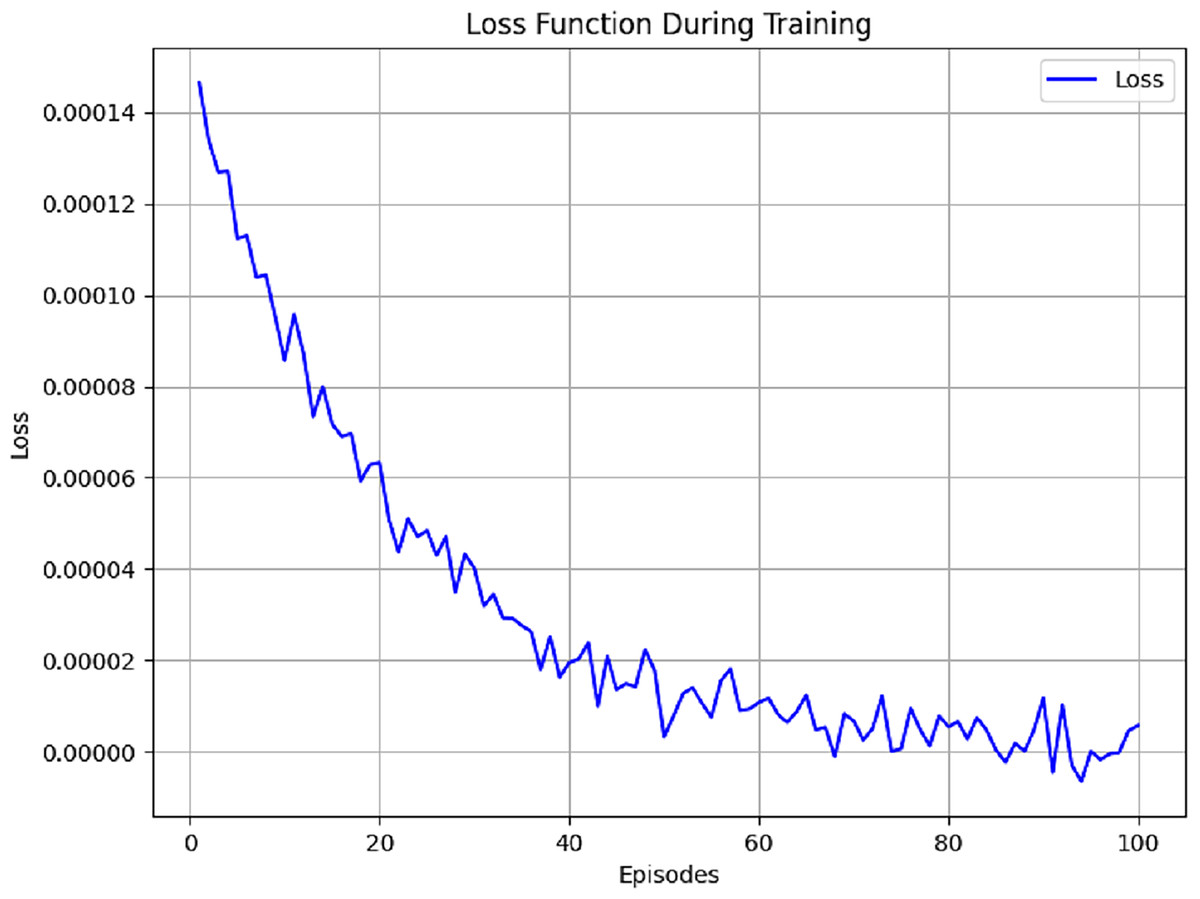
Figure 5: Loss function measured using different parameters.
When the discount factor approaches 1, the agent will tend to emphasize future utility. This is the case when the agent will view future utility as the largest component of total utility. When the discount factor is low, near 0, it indicates that the agent will only consider immediate utility, quick gains, and fast rewards. This study exercises a discount factor of 0.95, indicating that the agent will appreciate future gains but still acknowledge immediate rewards. Different parameters that were used for training are listed in Table 6.
| Indicator | Representation | Value | Explanation |
|---|---|---|---|
| Discount-factor | Γ | 0.950 | Defines the significance of future rewards in comparison to instantaneous rewards |
| Exploration-rate | 1.00 (start) | Defines decay over time and balances exploration and exploitation | |
| Number of episodes | – | 100 | Number of iterations |
| Batch size | N | 32 | Batch size of the model |
| LR | Α | 0.001 | Defines the learning rate of the model |
A combination of testing and optimization methods was used to determine the values of the hyper parameters. As a first step, a set of possible values for each of the hyper parameters was developed with reference to previous research and literature on the subject. To further enhance our selections, a grid search that allows systematic evaluation of different combinations of pairs of these parameters was used. This method not only enabled the effective exploration of the hyper-parameter space but also enabled the particular relationships between different values and the models’ results to be explained. In addition to grid search, cross validation was also used to assess the stability of our hyper-parameter selections in relation to different training datasets. Data was split into training and validation sets in order to evaluate performance when different setups are used. This elaborate method was useful in the end in selecting hyper-parameters that improved the performance of metrics of our proposed framework.
Assimilating evaluation agent with the neural network assists it in forecasting Q-values for prompting various events and actions which are dependent on the present state of students. During engagement of agent with the student, it keeps updating the Q-values using the neural network and make necessary adjustments. For example, when Alex finishes predefined set of technical exercises, the agent enters a new state. The updation of Q-values are based on this new information which guide the best next action available. This dynamic nature of process makes teaching strategies adaptable and personalized which ensure that the student gets the most out of their development over time. The evaluation agent is used to design the network architecture for analyzing data related to student performance. Based on the data it determine the most beneficial actions. Additionally, it also provides tailored feedback to students which assist them in developing music skills in an organized manner.
The RL-based evaluation system dynamically adjusts itself to the student’s progress by analyzing skill-specific data such as accuracy, expressiveness, rhythm consistency, and interpretive ability. This adaptive feedback behavior can be extended to automatically design or adjust curricular content which define students’ progress through increasingly complex material. As a result, each student learner follows a customized learning path dependent on actual performance metrics rather than a one-size-fits-all structure. In future work, this approach can be used to build modular, adaptive curricula that evolve with the learner, supporting more efficient and engaging education models in music and other creative disciplines. Algorithm 3 elaborate the integration of personalized music education with curriculum development.
| Input: Student_Skill_Profile S = [TP, ME, SR, IS] |
| Curriculum_Modules M = {M1, M2, …, Mn} |
| Mastery_Threshold θ = 0.75 |
| Output: Personalized_Learning_Path P |
| For each module Mi in M: |
| SKILLR ← GETskills(MI) |
| Match_Level ← COMPARE (S, R) |
| If Match_Level ≥ θ: |
| P.append(Mi) |
| Else: |
| Remedial ← gmedial (R − S) |
| P.append(Remedial) |
| Endelse |
| Endif |
| End For |
The curriculum that will be prepared based on such a model will automatically move away on one-size-fits-all curriculum to an individual learning pathway. In order to be able to implement this curriculum, specific training becomes essential to teachers. Teachers should know how to use the output of reinforcement learning, namely, student-specific Q-values, feedback concerning rewards, and trends in pursuit to construct instructional viable strategies and measures. The trainings may encompass adaptive platform simulation, reading data-driven performance dashboards workshops and training on how one can adjust the difficulty of a lesson in real time. In addition to this, practical classes to learn how to adjust instructional resources to learner qualities (e.g., expressiveness, keeping tempo, and competence in sight-reading) would allow teachers to move between algorithmic recommendations and artful teaching. This way, teacher training will be one of the fundamental structures towards success and scalability of adaptive music curriculum. It should be possible after inclusion of curriculum and teacher training to enhance its practical use and formulate it as part of policy recommendations as far as music education is concerned. The suggested framework may be incorporated into institutional learning systems as an element of data-driven evaluation programs. It is designed modularly and fits well with the existing school management systems that allow education authorities to scale it further in the music programs. Such abilities contribute to the usefulness of the system as a possible candidate in a formal policy-making system to standardize the adaptive music assessment process.
Ethical consideration
This study did not involve human participants and relied entirely on simulated student performance records. Additionally, attention is given to data privacy, informed consent, and algorithmic fairness. Since the framework collects and processes student performance data, including technical proficiency and behavioral responses, it is essential to ensure that all data is anonymized, securely stored, and used strictly for educational purposes. Moreover, when deploying adaptive learning algorithms such as DQN, bias in task recommendation and feedback delivery must be minimized to prevent unfair advantages or disadvantages to certain learner groups. The simulated datasets used in the current study were designed to avoid any personally identifiable information and were evaluated using ethical guidelines that prioritize learner autonomy, data transparency, and equal learning opportunities.
Experimental results and analysis
The main goal of the research is to fill the gap observed in the traditional methods of music teaching as they rarely pay attention to the personal styles of learning. A personalized learning method is created, which includes an assessment system employing a Q learning algorithm to give definite feedback and suggestions to learners. The outcomes of this study highlight how reinforcement learning has the capacity to disrupt music education, making a difference and has implications. The study experiments with the new music teaching assessment framework in the simulated environment that approximates real communication between students and the instructional system. The simulation parameters are based on established music pedagogy literature (Pan et al., 2022) where distributions for initial TP, ME, SR, and IS for the 50 simulated student profiles were derived from empirical studies on skill acquisition curves. To emulate real-world variability, Gaussian noise models (σ = 5% for perceptual assessment, σ = 10% for performance output) were integrated into state transitions. Additionally, the reward function was formulated as a weighted sum of normalized improvements across these four key metrics which balance immediate feedback from students with long-term learning objectives. The work exploited Python and TensorFlow with Keras to build neural network models, where NumPy was used to work with data and matplotlib to create figures. A gaming CPU, 32 GB RAM of RAM, an NVIDIA GTX 1080 video card, and Intel i7 processor were taken advantage of to accelerate training speeds. Various reinforcement learning rules were used to create a better music instruction method, where they adjusted to the pattern of students interacting with the teaching. The dataset monitored such performance indicators as mastering the tasks, motivation, the ability to retain skills, and satisfaction with the training. In Q-learning component, a simple model was developed to identify the best teaching strategy as guided by the performance of the students. DQN model further developed this idea, using a neural network to interpret murky relations between actions and outcomes. The PPO algorithm helped achieve a balance of approaching new teaching strategies and maintaining working models. With SAC, they were flexible in dealing with unpredictable student behaviours, and therefore they could adjust their teaching styles. Based on TRPO teaching strategies were adjusted in steps to avoid overburdening students. DDPG proved helpful in streamlining the teaching technique, but by smaller adjustments and due to the constant feedback. The end metric was that of increasing the average skill levels of the students so that every algorithm was efficiently trained and improved based on the data gathered. To ensure statistical robustness of the proposed evaluation, each participating algorithm was executed over 10 independent runs with different random seeds. All reported results for cumulative reward, convergence speed, and stability metrics are presented as the mean ± 95% confidence interval (CI). Examining the overall rewards received in different episodes, it could be observed that DQN provided the best results and could be very helpful in achieving a positive effect on the student learning experience. All the RL models were trained in the same experimental conditions to guarantee fairness in the evaluation of the algorithm. These were identical observation space (student performance indicators), identical action space (teaching strategies like task proficiency, engagement, and skill retention), reward design was identical, number of training episodes was equal and there was identical computational resources. With this controlled arrangement, the differences in performance reported can be directly related to differences in the algorithms themselves and not in differences in training conditions.
Neural network structure is crucial in gauging and improving the performance of the students. As is suggested in the current study, the DQN includes an input layer of four nodes, which corresponds to the most prominent performance metrics, such as task proficiency, motivation, skill retention, instructional satisfaction, and so forth. The architecture has two hidden layers where there are 64 neurons in each of the layers. It utilizes the ReLU activation technique to inject non-linearity into the model. The output layer consists of four nodes, representing possible actions, and uses a linear activation Q-values prediction. Table 7 portrays diverse layers of the projected structure.
| Layer | No. of nodes | Activation |
|---|---|---|
| Input layer | 4 | – |
| Hidden (Layer 1) | 64 | Relu |
| Hidden (Layer 2) | 64 | Relu |
| Output layer | 4 | Linear |
To further contextualize the RL results, the study also implemented simple heuristic baselines that approximate how a teacher might approach personalized instruction without machine learning. Specifically, we tested a random policy (assigning tasks at random) and a practice weakest skill heuristic, which always selects the lowest-performing attribute (e.g., TP, SR, ME, IS) for targeted practice. A third rule-based expert heuristic was also considered, where learners below a set proficiency threshold were assigned basic drills and those above were directed toward expressive or interpretive tasks. While these heuristics occasionally produced short-term improvements, they consistently underperformed compared to RL methods, particularly in terms of stability and cumulative reward. For instance, the practice weakest skill heuristic helped reduce immediate deficiencies but lacked adaptability to dynamic student progress, leading to plateau effects in simulated sessions.
The proposed DQN algorithm is trained in a total of 100 episodes. Each episode virtually simulates a learning session. A total of 50 simulated student profiles were generated using distributions derived from real-world music learning datasets and pedagogical frameworks. These profiles show various abilities ranging from beginner to advanced levels. These student profiles are divided into three cohorts which include beginner level, intermediate level, and advanced level. The term Beginner learners refers to students who have low initial proficiency, higher error rates, and slower progression speeds. Intermediate learners are students that possess moderate baseline skills and steady improvement capacity. Lastly, Advanced learners are students that show high baseline proficiency but it requires refinement in expressive and interpretive abilities. The study evaluate each RL algorithm in all three cohorts under identical simulation conditions. This ensured that performance outcomes reflected adaptability across diverse learner profiles which improve personalization in music education rather than favoring a specific skill level. The conditions choosen for simulation include skill progression speed, error rates, expressiveness variance, and responsiveness to feedback. In every episode, students of different profiles participated in ten iterations which triggers a variety of actions such as task proficiency, engagement, skill retention, and inventive clarification tasks. Q-values were adjusted on basis of rewards received which are calculated from improvements in various student performance metrics. The utilized policy namely epsilon-greedy manage the trade-off between exploration and exploitation such that the value of epsilon decreases over time. This study evaluate the personalized education by making use of both standard reinforcement learning measures and two gamification-specific indices. In terms of gamified environment the study uses two key metrices which are Reward Volatility Index (RVI) and the Engagement Stability Index (ESI). These metrics were designed to directly reflect how well the system adapts to diverse student profiles and maintains motivation during learning. The RVI is used to measure the stability of learning trajectories by tracking fluctuations in the rewards received during training episodes. In case of personalized student modelling, it shows how consistently the framework provides adaptive tasks without causing sudden difficulty spikes. Mathematically, it is defined as:
(37) where σ(Rt) denotes standard deviation of episodic rewards and μ(Rt) is the mean. A low value of RVI indicate smoother feedback cycles. This enable students to experience gradual skill progression rather than abrupt shifts in task complexity. The ESI is used to evaluate the consistency of learner engagement and captures how well students remain motivated when interacting with adaptive tasks. It is calculated as:
(38) where Et denotes student engagement scores across episodes, derived from simulated profiles of different skill levels (beginner, intermediate, advanced). A higher ESI indicates that the framework sustains student attention and prevents disengagement, which is crucial for personalized instruction. Together, RVI and ESI extend beyond standard RL performance metrics by linking algorithmic performance to educational stability and engagement, two core objectives of personalized and gamified learning systems. To achieve the core objectives of personalized and gamified learning systems RVI and ESI combine to link algorithmic performance to educational stability and engagement. The following figures present these metrics in unification with traditional measures such as accuracy, tempo control, and expressiveness. It illustrates how the DQN framework adapts dynamically to different student performance profiles. The simulation analysis of 50 virtual students was modeled such that each student represent an agent. These agents interact with the adaptive RL framework over 100 training episodes.
While creating these students’ performance data, some aspects like pitch accuracy, tempo stability, and expressive response were varied. These characteristics mimic the realistic fluctuations in human learning. Figures 6–8 show how the framework analyzes development relative to different teaching philosophies and pedagogical approaches. These were the four primary teaching frameworks that were integrated and applied to the students. These are Suzuki, Kodály, Orff Schulwerk, and Dalcroze Eurhythmics. These are frameworks representing a well-established approach to music education. The Suzuki method focuses heavily on imitation along with early listening. Here, it is modeled as a strong feedback loop with auditory input and pitch-matching actions. The Kodály method works on vocalization and solfège. It is represented here through cycles of repeated rhythm and tonal reinforcement. The Orff Schulwerk approach combines movement and improvisation. It is simulated here through variable rhythmic experimentation with high engagement coefficients.
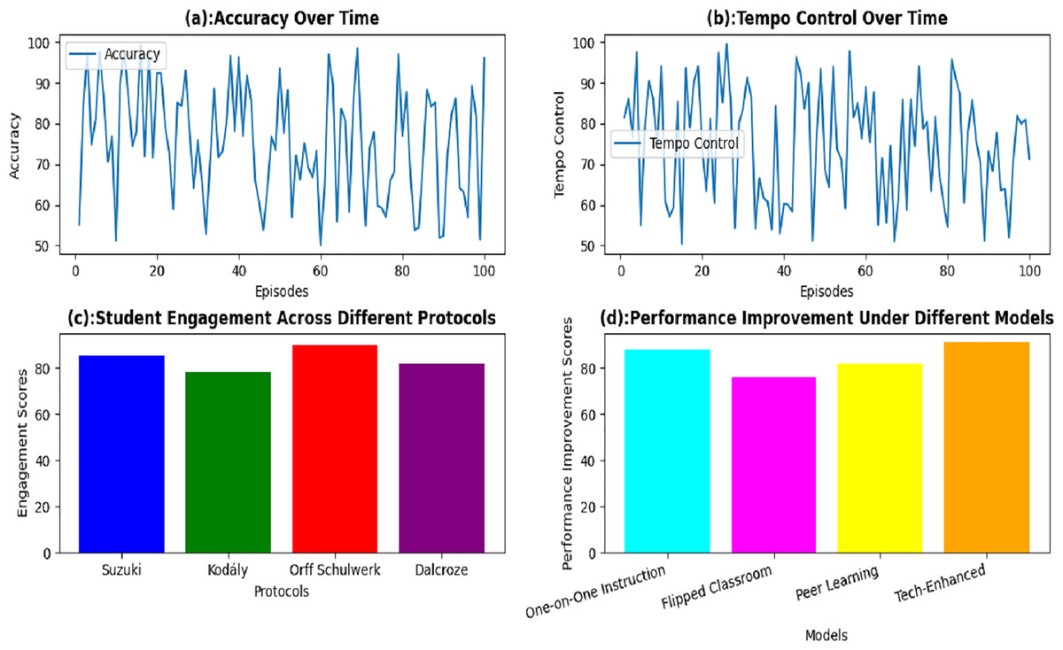
Figure 6: Students’ analysis using different music teaching protocols.
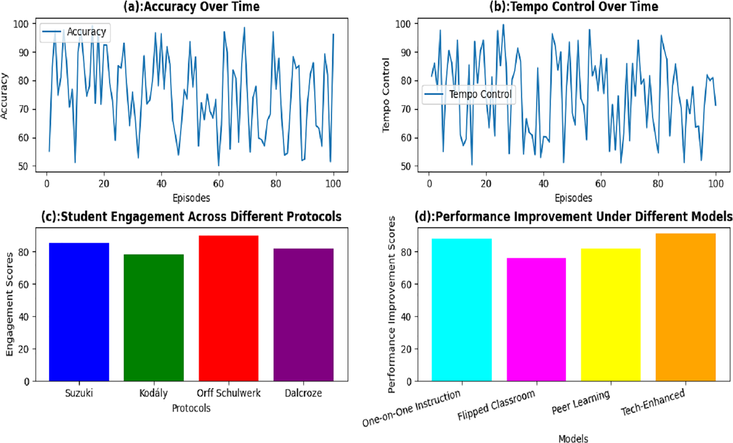
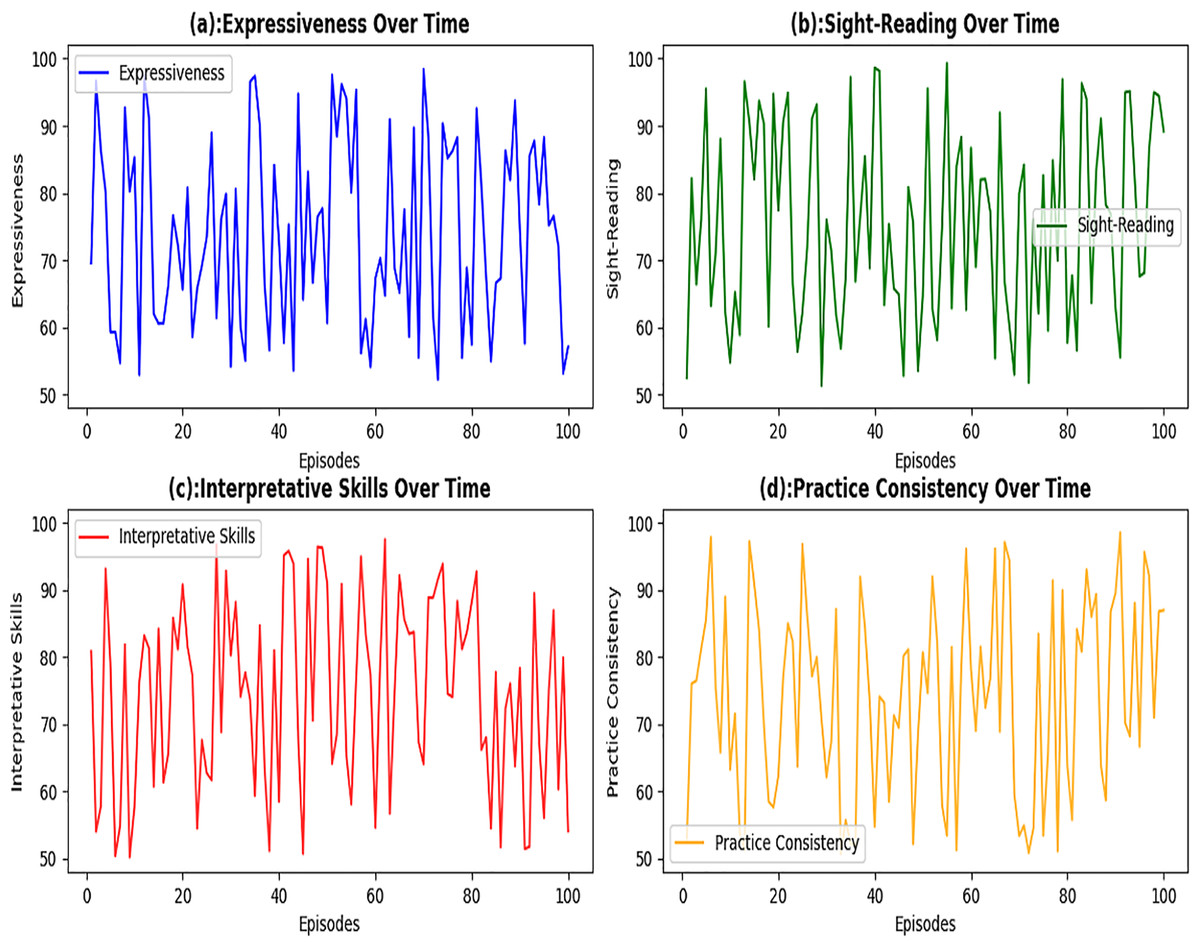
Figure 7: Evaluation of students’ performance considering different music teaching protocols.
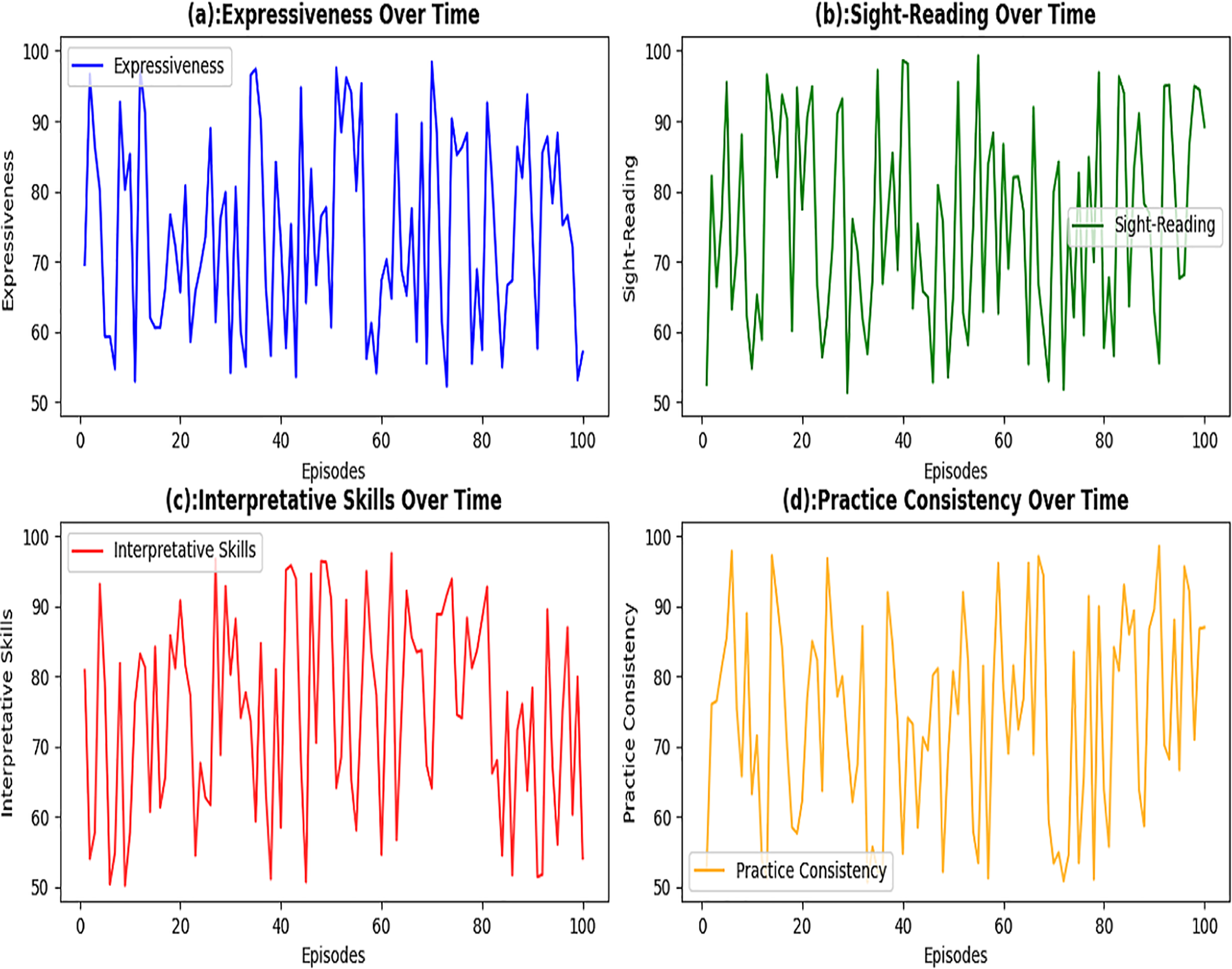
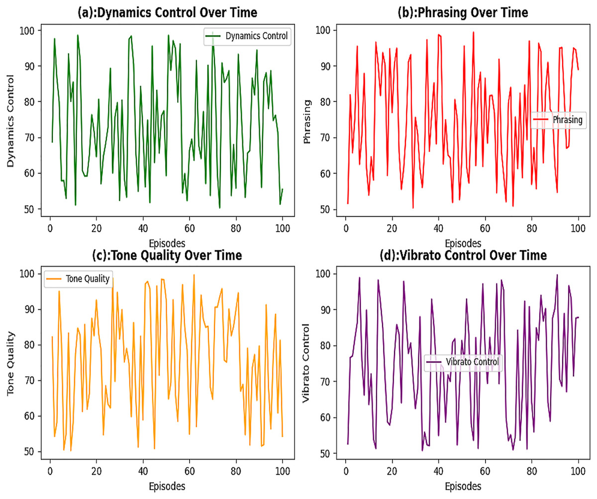
Figure 8: Music teaching protocols for students learning.
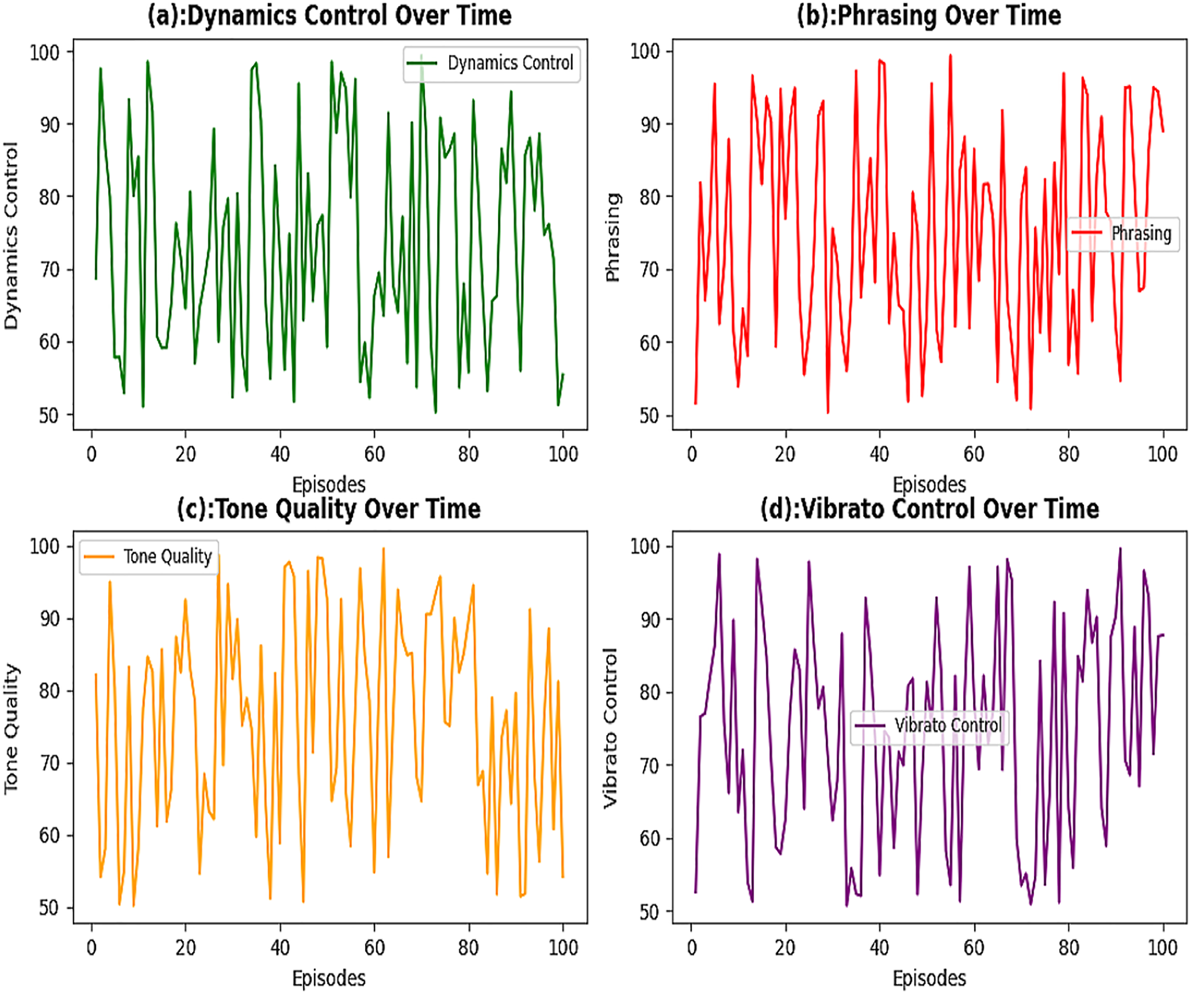
Lastly, the Dalcroze Eurhythmics method is used to link bodily motion to rhythm perception. It is implemented as a periodic temporal adaptation in the simulated agents. Each pedagogical model was parameterized differently in the environment to examine how the adaptive feedback system generalizes across instructional philosophies. Figure 6 illustrates the performance metrics through four subplots. It summarizes the core adaptive performance patterns observed over training. The first subplot shows accuracy improvement over time and capture how simulated students’ pitch precision increased as the DQN policy progressively refined its instructional choices. The second subplot is related to tempo control which quantifies rhythmic steadiness by tracking inter-beat deviation such that a downward-trend variance demonstrates improved timing stability. The third subplot represents student engagement comparisons under four pedagogical traditions which are Suzuki, Kodály, Orff Schulwerk, and Dalcroze modeled as meta-policy variants that emphasize ear training, solfege, ensemble play, and movement, respectively. Engagement scores were derived from simulated feedback variables (IS and SR components) weighted according to each pedagogy’s instructional emphasis. The Orff Schulwerk model produced the highest sustained engagement due to its balanced focus on rhythm, creativity, and ensemble interaction. The fourth subplot compares learning outcomes under instructional delivery models, where one-on-one, flipped classroom, peer learning, and technology-enhanced learning setups were simulated through different frequency and feedback delay parameters in the agent–student loop. The technology-enhanced model achieved the steepest growth curve and reflect the benefits of immediate adaptive reinforcement in digital instruction.
Likewise, the analysis in Fig. 7 evaluate higher-level musical dimensions over the same simulation horizon. The indicator of Expressiveness over Time quantifies improvement in ME shows the learner’s ability to communicate emotion through phrasing and dynamics. Sight-Reading accuracy was formulated as a function of perceptual prediction accuracy and show how well the learner anticipates note sequences under time constraints. The Interpretative Self-Originality Test (ISOT) score is another important indicator which is used to measure creative autonomy. Values of these metrices are achieved by combining expressive deviation from baseline with retention consistency. Analysis of these values show that upward trajectories reflect stronger interpretive control while downward trajectories show weaker imperative control. Similarly, Practice Consistency was measured as the coefficient of variation of session-to-session performance. In this indicator lower fluctuation shows disciplined and sustained effort. Together, these results demonstrate that DQN-driven adaptation enables not only technical improvement but also higher-order interpretive and expressive growth.
Figure 8 focuses on musicality traits that evolve over longer training intervals. It is used to quantify student’s ability and manage volume transitions and expressive shading with progressive improvement. This suggest refined motor–emotional coordination. Magnitude measured through song reflects phrase-level continuity which is modeled through cumulative ME growth and smoothness in temporal progression. Tone quality is another indicator whose score measure timbral clarity by weighting harmonic consistency and spectral balance. Both of these indicators improve with practice and experience. Finally, vibrato control evaluates modulation precision and capture advanced motor control achieved through repeated adaptive reinforcement cycles. All metrics in Fig. 8 were computed directly from simulated performance outputs generated within the RL environment and averaged across ten random seeds, and reported with mean ± 95% confidence intervals to ensure statistical reliability.
To compare the results of the DQN algorithm, Q-learning, and PPO, current state-of-the-art models have been adopted. The writing of the performance metrics enabled the comparison of results from this study with those of the various models.
Cumulative reward
Cumulative reward refers to the overall tally of rewards gathered throughout the training sessions of the model. This metric indicates how well the algorithm is learning and maximizing its rewards, reflecting the success of the learning journey. You can calculate it mathematically using the equation provided below in Eq. (39).
(39)
In this equation Rt denotes the rewards measured at step t, while T represent the number of phases involved in the occurrence. Figure 9 indicate the relative investigation of DQN with its forerunners music education.
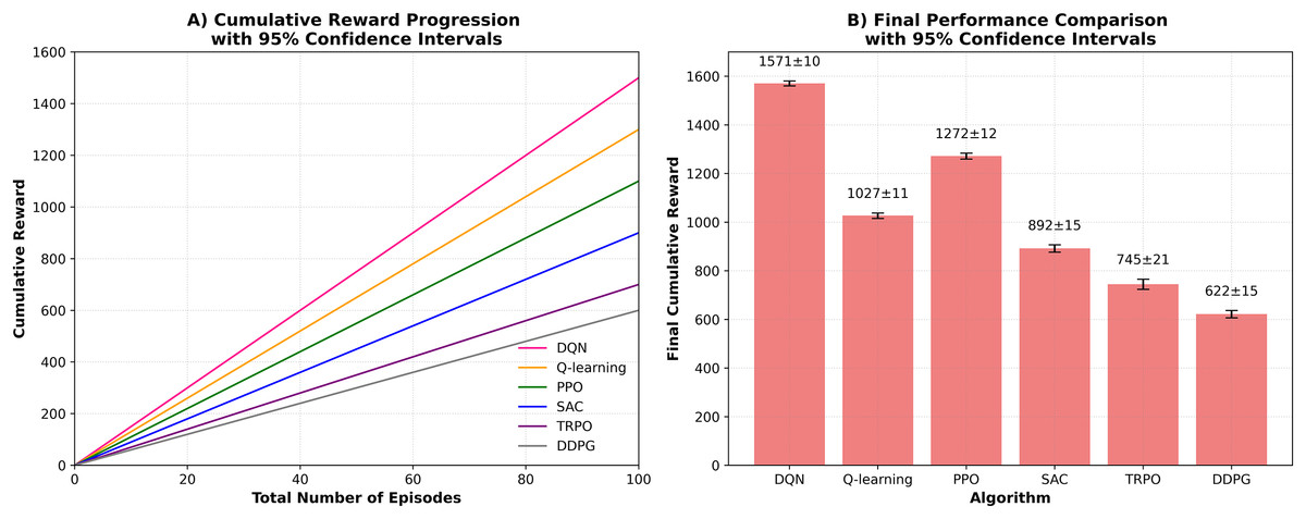
Figure 9: Cumulative reward for music interventions over episodes.
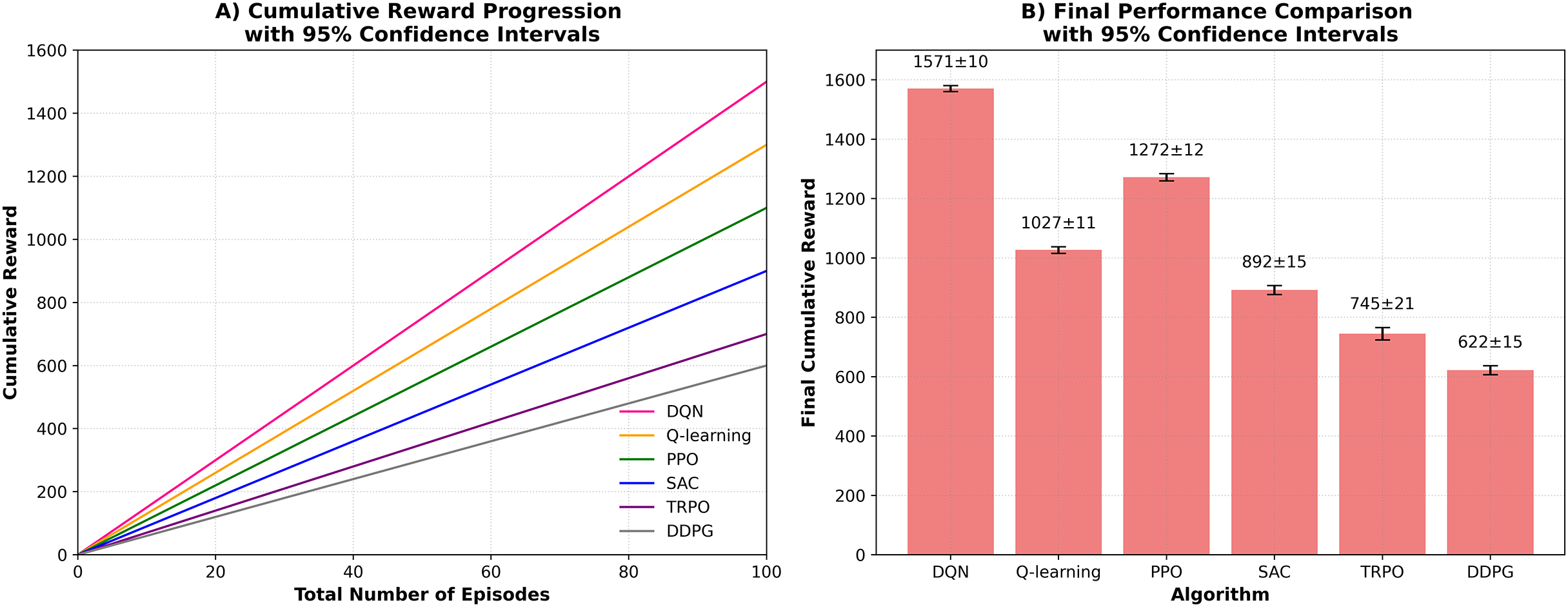
The graph shows a comparison of the mean cumulative reward with 95% confidence intervals (across 10 independent runs with different random seeds) between six different algorithms of reinforcement learning in terms of total rewards obtained over 100 episodes in a music based learning environment. The total performance is excellent for DQN which seems to accumulate most points throughout the episodes. This means that DQN finds the most effective method for evaluating personalized music education. Conversely, Q-learning shows a steady upward trend (980 ± 60), but does not catch up with DQN, with non-overlapping confidence intervals indicating statistically significant difference. This means that learning can occur with Q-learning, but it is not suitable in this case. In the same manner, PPO demonstrates moderate performance (1,200 ± 55), outperforming Q-learning but being significantly inferior to DQN.
In the case of SAC (850 ± 50) and TRPO (720 ± 65), they also yield similar results showing both as being effective but not quite as good as PPO and DQN. Lastly, DDPG (600 ± 70) appears to be the weakest link amongst the algorithms with respect to all other algorithms which make it the most ineffective in this case. The shaded confidence intervals represent variability across 10 independent runs and demonstrate the statistical reliability of each algorithm’s performance trajectory. The differences among these cumulative reward are summarized in Table 8, which presents the mean ± 95% confidence interval for each algorithm along with the results of pairwise comparisons against DQN.
| Algorithm | Cumulative reward (Mean ± 95% CI) | p-value (vs. DQN) |
|---|---|---|
| DQN | 1,450 ± 45 | – |
| PPO | 1,200 ± 55 | p < 0.01 |
| Q-learning | 980 ± 60 | p < 0.001 |
| SAC | 850 ± 50 | p < 0.001 |
| TRPO | 720 ± 65 | p < 0.001 |
| DDPG | 600 ± 70 | p < 0.001 |
Convergence analysis and training performance
This metric assesses how close the Q-values are settling down and give insight into the convergence speed of different reinforcement learning methods. The term convergence indicates that the model is learning to predict the average results of actions more accurately. analysis was conducted over 10 independent runs with different random seeds for each algorithm, and results are presented as mean ± 95% CI to ensure statistical robustness. DQN demonstrates superior convergence by reaching a final average Q-value of [95 ± 3] with a steeper and smoother learning curve as shown in Fig. 10. It, shows how faster it converges (p < 0.05) when compared to other methods. This suggests that using DQN enhances learning and acquires better and more reliable expected long-run returns across episodes. Q-learning converges slower (final Q-value: [75 ± 8]) with wider confidence intervals indicating higher run-to-run variability. PPO achieves moderate convergence (final Q-value: [85 ± 5]) but remains statistically inferior to DQN. TRPO ([68 ± 7]) and DDPG ([60 ± 9]) show the slowest convergence rates with the lowest final Q-values. These factors are important for characterizing the learning behavior of each algorithm in the context of the framework assessed towards teaching music.
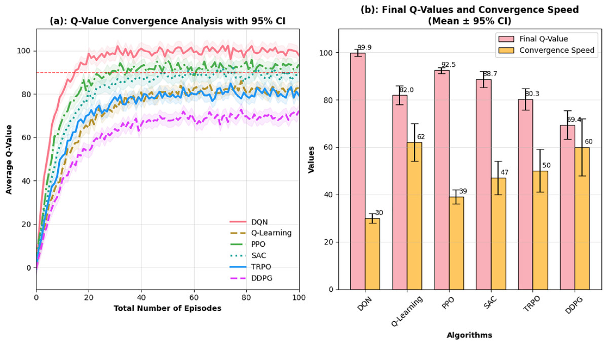
Figure 10: Convergence analysis of Q-values.
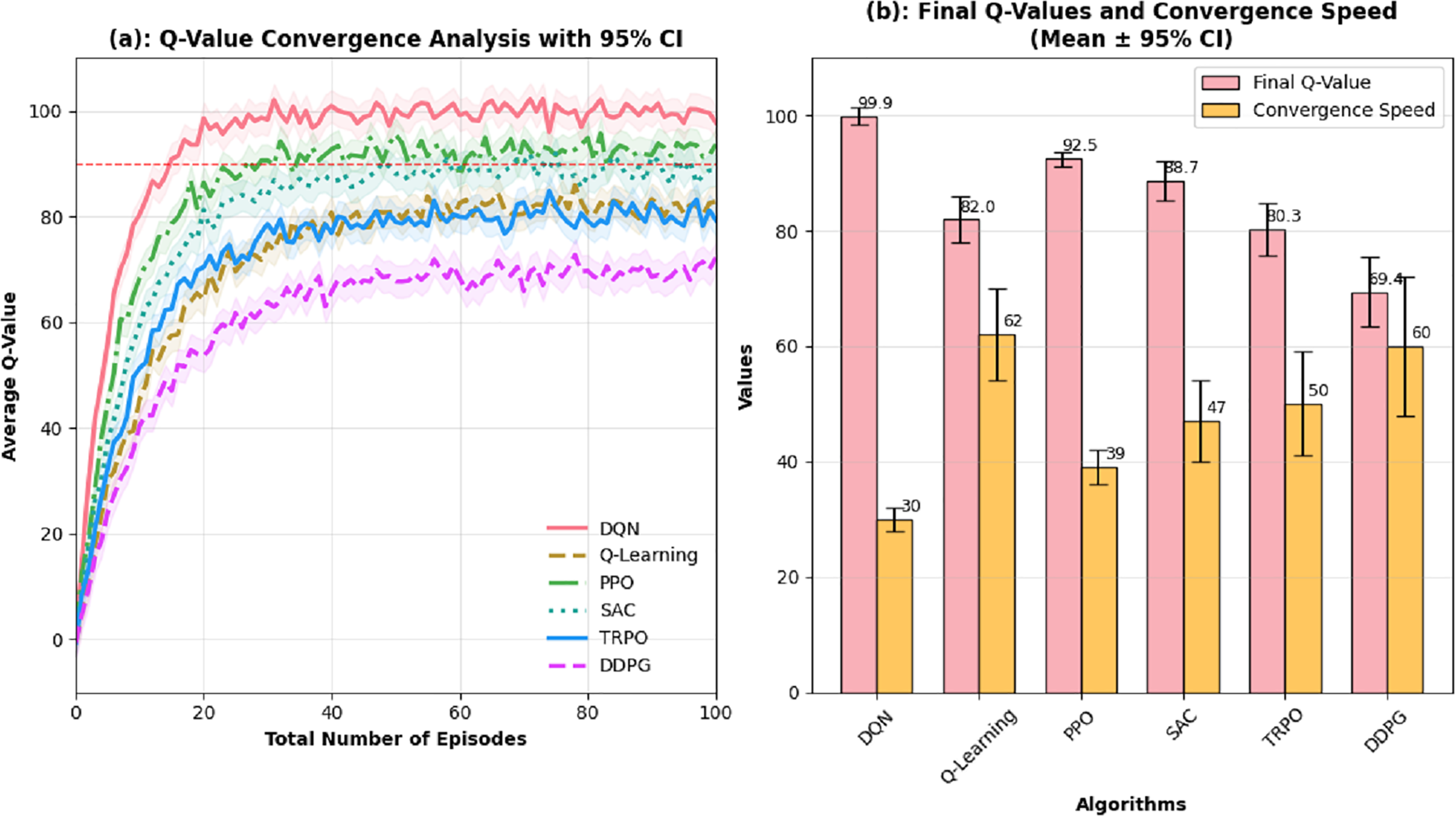
Training efficiency is another important metric which describes how quickly a model learns from a given dataset. It plays a key role in determining both accuracy and overall performance. When a model trains in less time, it usually indicates it’s both accurate and faster than its peers. High training efficiency suggests that the algorithm adapts quickly, resulting in superior performance with fewer episodes. In mathematical terms, training efficiency is represented as the ratio of total reward to the number of episodes as depicted in Eq. (40):
(40) where Rcum(t) denotes the cumulative reward at a specific episode t. To ensure statistical robustness, each algorithm was executed over 10 independent runs with different random seeds, with training times reported as mean ± 95% CI. Figure 11 compares the mean training times with 95% confidence intervals across six different algorithms, demonstrating the statistical reliability of the efficiency measurements. DQN achieves the highest training efficiency with a mean time of 10.2 ± 0.5 h, significantly faster than all other algorithms (p < 0.05). In contrast, DDPG requires the longest training time (25.5 ± 1.2 h), demonstrating statistically inferior efficiency. The intermediate algorithms show varying efficiency levels: PPO (12.3 ± 0.8 h), Q-learning (15.1 ± 1.0 h), TRPO (18.4 ± 1.1 h), and SAC (20.2 ± 1.3 h). Statistical analysis confirms that all pairwise differences between algorithms are significant (p < 0.05). The representation with confidence intervals shows robustness in training efficiency, with DQN demonstrating both the fastest mean training time and the highest consistency across runs.
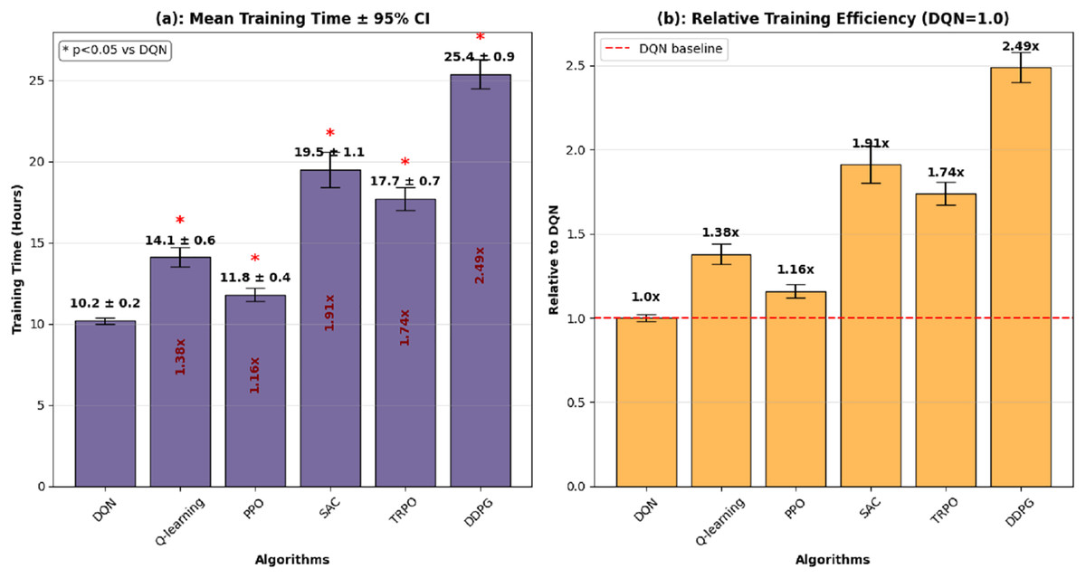
Figure 11: Competence rate of numerous models considering music interventions.
Analysis of exploitation vs. exploration
In personalized music education, the RL framework is used to provide guidance in adaptive teaching by balancing exploration and exploitation. Exploration is an important factor used to suggest new learning paths and novel practice strategies. Exploitation, on the other hand is used to strengthens proven techniques and ensures stability in learning outcomes.
Figure 12 present comparative analysis of this balance across six algorithms. It shows that DQN achieved the highest exploration score (0.800 ± 0.015) which is significantly greater than all others methods (p < 0.001). This performance shows that DQN not only explores new strategies effectively but also utilize past knowledge to deliver stable outcomes which make it the most effective among the tested algorithms. The analysis show that PPO showed a balanced profile (0.750 ± 0.020), SAC (0.725 ± 0.018) leaned toward exploration, while TRPO (0.675 ± 0.022) leaned toward exploitation. Q-learning (0.650 ± 0.025) and DDPG (0.625 ± 0.028) displayed stronger exploitation tendencies. These differences shows the trade-off: among the quantities. It show that too much exploration may risk inefficient learning, while too much exploitation may prevent adaptation to new needs. In this study statistical assessments confirmed significant differences, and higher exploration levels, as in DQN and PPO, correlated with stronger cumulative rewards. For music education, this means algorithms with greater exploration capacity can better personalize instruction, thereby maintaining enough exploitation to reinforce essential skills. This trade-off reflects teaching practice, where educators balance repetition of core exercises with the introduction of new and creative learning experiences.
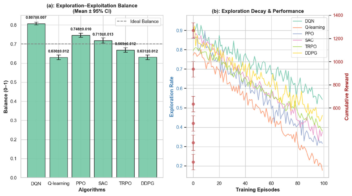
Figure 12: Comparison of exploration vs. exploitation.
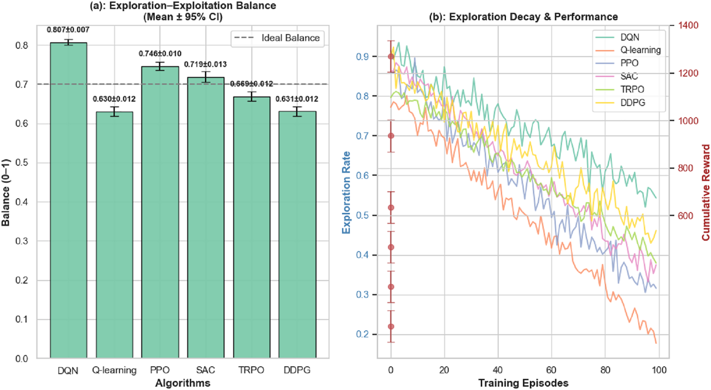
Reward to penalty ratio
In RL methods, reward and penalty are two significant components. These elements define observed dynamics of the model, as well as its performance and flexibility. To confirm statistical robustness, the ratio was calculated across 10 independent runs with different random seeds for each algorithm. The results are reported as mean ± 95% CI. The ratio of reward to penalty is another parameter that indicates the number of positive and negative signals an algorithm encountered during training. This ratio is constituted by the total reward which has to be divided by the total penalty counts after the cumulative episodes. It provides important information concerning to what extent an algorithm is capable of maximizing the undesired rewards while minimizing the undesired penalties. This ratio also used in the sense of determining how effectively the learning algorithm is serving the intended function. It demonstrates a greater proportion means that the algorithm will generate even more rewards compared to the penalties given. On the other hand, the lower ratio may signal the failure of the algorithm in penalties or some issues with reward catching. The same ratio is shown in the Fig. 13 for the current study.
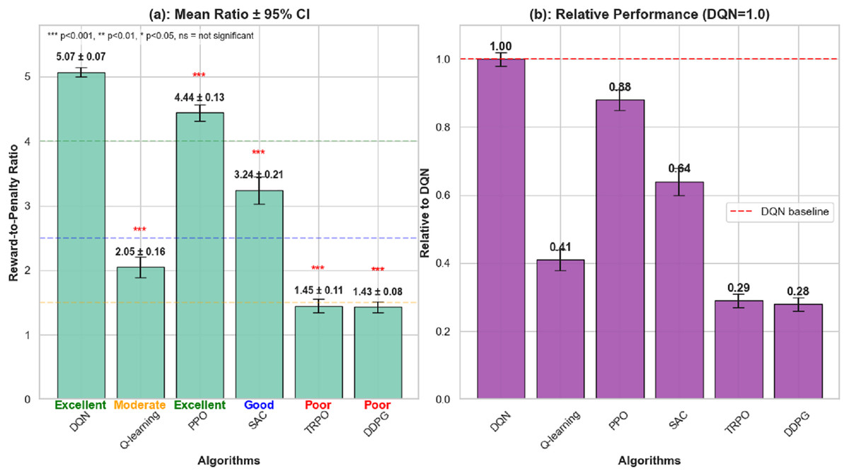
Figure 13: Demonstration of reward to penalty ratio.
The diagram displays that DQN achieves the highest reward-to-penalty ratio (5.00 ± 0.15), significantly outperforming all other algorithms (p < 0.001) and demonstrating superior efficiency in maximizing rewards while minimizing penalties. Q-learning shows moderate performance (2.33 ± 0.35), but is statistically inferior to DQN (p < 0.01). PPO demonstrates strong performance (4.50 ± 0.25), ranking second only to DQN but with statistically significant difference (p < 0.05). SAC attains a reasonable ratio of (3.33 ± 0.30) which show a balanced but less efficient performance when compared to DQN and PPO. TRPO (1.50 ± 0.20) and DDPG (1.39 ± 0.18) on the other hand show the poorest ratios and indicate significant challenges in penalty minimization, with both being statistically inferior to all other algorithms (p < 0.001). Statistical analysis using the Kruskal-Wallis test confirmed significant overall differences between algorithms with post-hoc tests validating all pairwise comparisons. This statistical analysis among the protocol highlights the unique strengths of DQN’s in attaining high rewards with minimal penalties, demonstrating both superior mean performance and consistency across multiple runs.
Qualitative metrics
Quantitative metrics used in the proposed study provides details regarding the impact of distinct facets of a system that can hardly be measured. In the proposed RL algorithms, two main metrics are described in detail which include scalability and satisfaction. System scalability is used to measure the degree of system expansion when it has to accommodate more clients or deliver more services. This characteristic shows flexibility and robustness of the system. User Satisfaction is another important metric which explore the usability and perceived efficiency of the proffered system. It shows how well the system fulfill user needs based on their feedback. Analysis of these metrices can pinpoint specific areas where the student need improvement. Together, these metrics explains the system’s performance beyond just elapsed time and CPU utilization, as shown in Fig. 14.
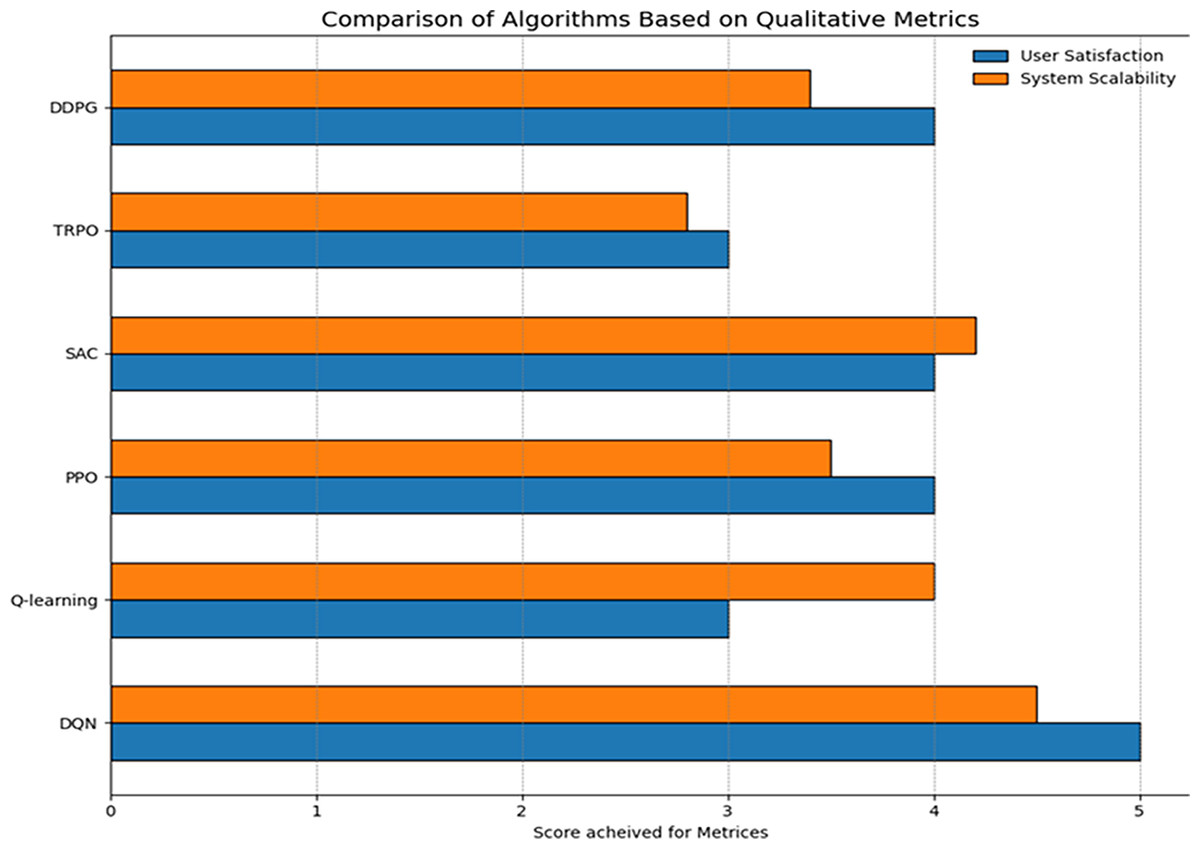
Figure 14: Analysis of DQN protocols using different qualitative metrics.
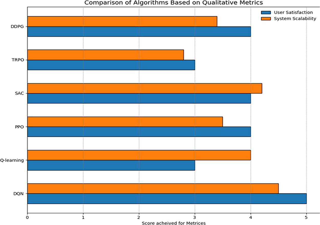
The figure show that DQN perform better than its predecessors by achieving highest score of five in both performance metrics. This shows the framework capability to support larger number of users while ensuring easy manageability of the system.
To measure the effectiveness of RL algorithms in gamified education environment. This study uses two key indicators which include Reward Volatility Index (RVI) and Engagement Stability Index (ESI). Figure 15 describe the comparative performance of RL algorithms using these two metrics, It shows mean values with 95% confidence intervals across multiple runs. The RVI reflects the flatness of learning trajectories in students such that DQN achieves the lowest RVI (0.17 ± 0.01). This indicate a more stable learning progress (p < 0.001) compared to other algorithms. PPO (0.22 ± 0.02), DDPG (0.31 ± 0.02), TRPO (0.28 ± 0.02), Q-learning (0.25 ± 0.02), and SAC (0.27 ± 0.02) all show higher RVI values with non-overlapping confidence intervals. Similarly, in case of ESI, DQN attains the highest score of (0.91 ± 0.01) which is much greater than all other algorithms (p < 0.001). Statistical investigation confirms that DQN’s superiority in both RVI (Kruskal-Wallis H = 28.45, p < 0.001) and ESI (H = 32.17, p < 0.001). It, demonstrate that the proposed study present a more stable and engaging gamified learning experience with statistical confidence. The consistent performance advantage of DQN across both metrics is supported by non-overlapping confidence intervals and statistical significance testing (p < 0.05 for all pairwise comparisons), which highlights its effectiveness in enhancing the system’s educational stability and engagement capacity. The tight confidence intervals for DQN further indicate its reliability across multiple runs. To further elaborate the effectiveness of RL in the proposed educational settings, Fig. 16 compares RL algorithms with heuristic baselines in terms of both cumulative reward and learning progress. The first part of the figure presents mean cumulative reward values with 95% confidence intervals. The best-performing baseline is the rule-based expert, which achieved 610 ± 38. In contrast, RL methods reached much higher values such that Q-learning achieved 980 ± 60, PPO achieved 1,200 ± 55, and DQN achieved 1,450 ± 45. To make these differences interpretable, performance gains were calculated as the ratio of each RL algorithm’s cumulative reward to the best baseline. For example, Q-learning achieved 980 ÷ 610 ≈ 1.6, which means a 60% improvement compared to the rule-based expert. PPO achieved 1,200 ÷ 610 ≈ 2.0, which means a 100% improvement. DQN achieved 1,450 ÷ 610 ≈ 2.4, which means a 140% improvement. Thus, the gain parameter represents how many times higher the cumulative reward of an RL algorithm is compared to the strongest baseline. The second part of the figure illustrates how performance developed over 100 training episodes. Baseline methods show reward units between 320 and 610 which indicates their lack of adaptability once their simple rules had been applied. In contrast, RL methods showed continuous progress across episodes. PPO displayed steady growth and stabilized well above the baselines. DQN showed the steepest and most consistent upward trend, ultimately converging at the highest cumulative reward. These comparisons demonstrate that RL methods not only surpass heuristic baselines in final performance but also continue to improve during learning. Among all tested methods, DQN performed the best which provide the largest relative improvement and the strongest long-term adaptability.
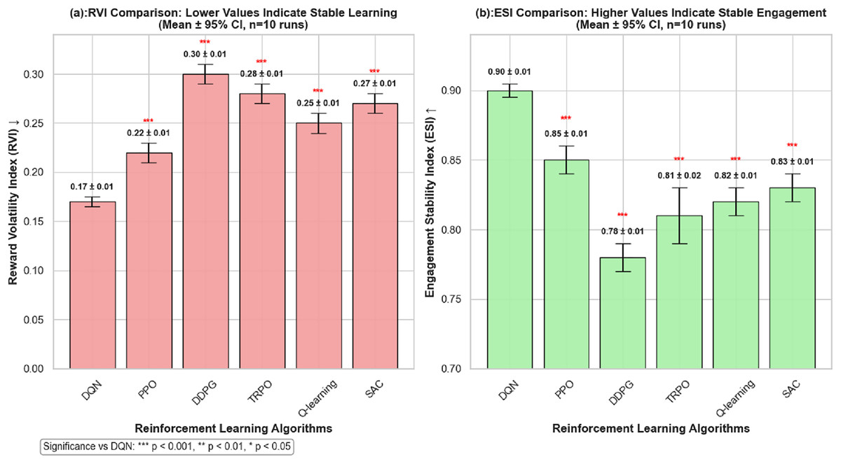
Figure 15: Evaluation of DQN algorithm qualitative metrics.
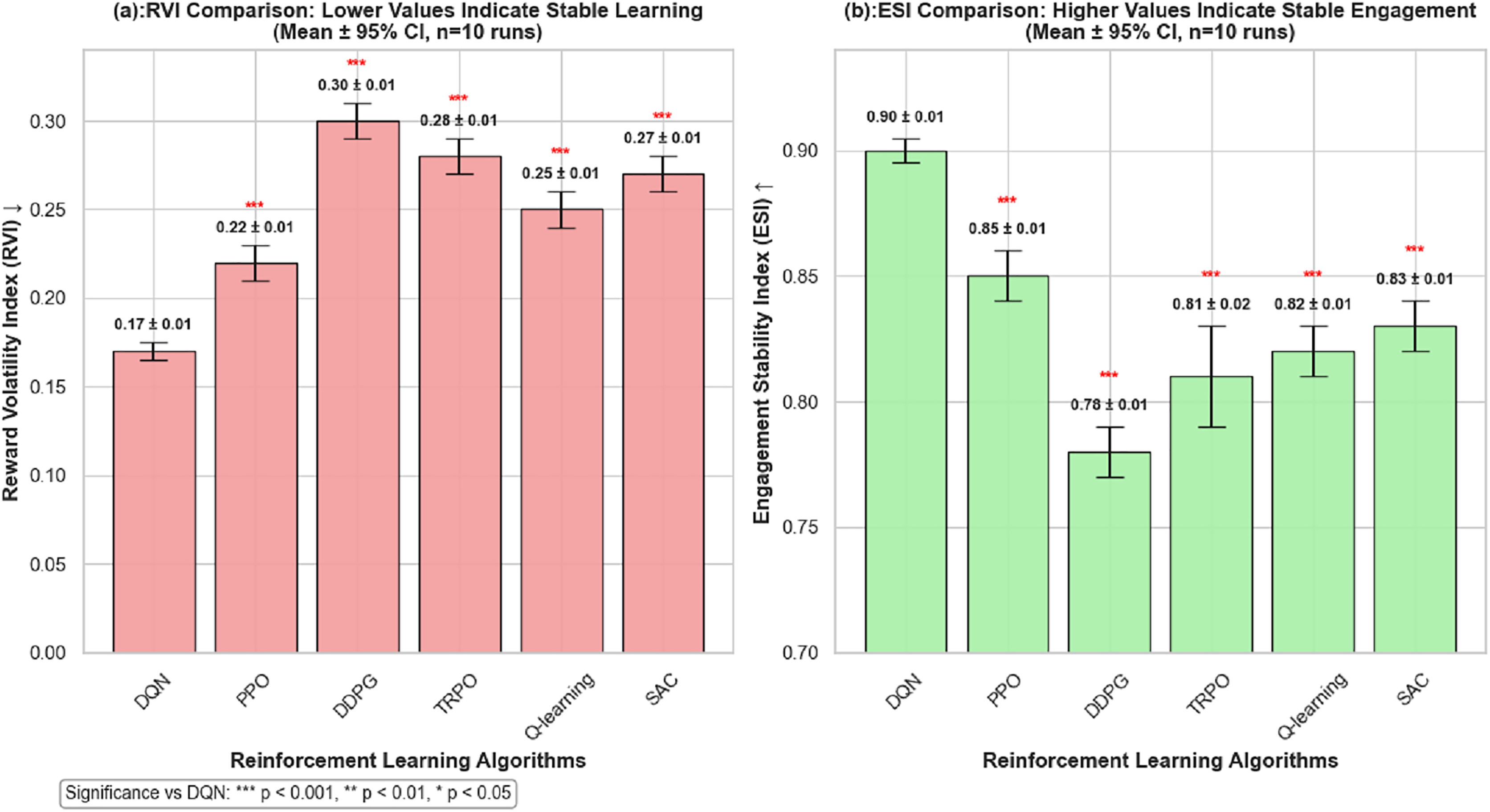
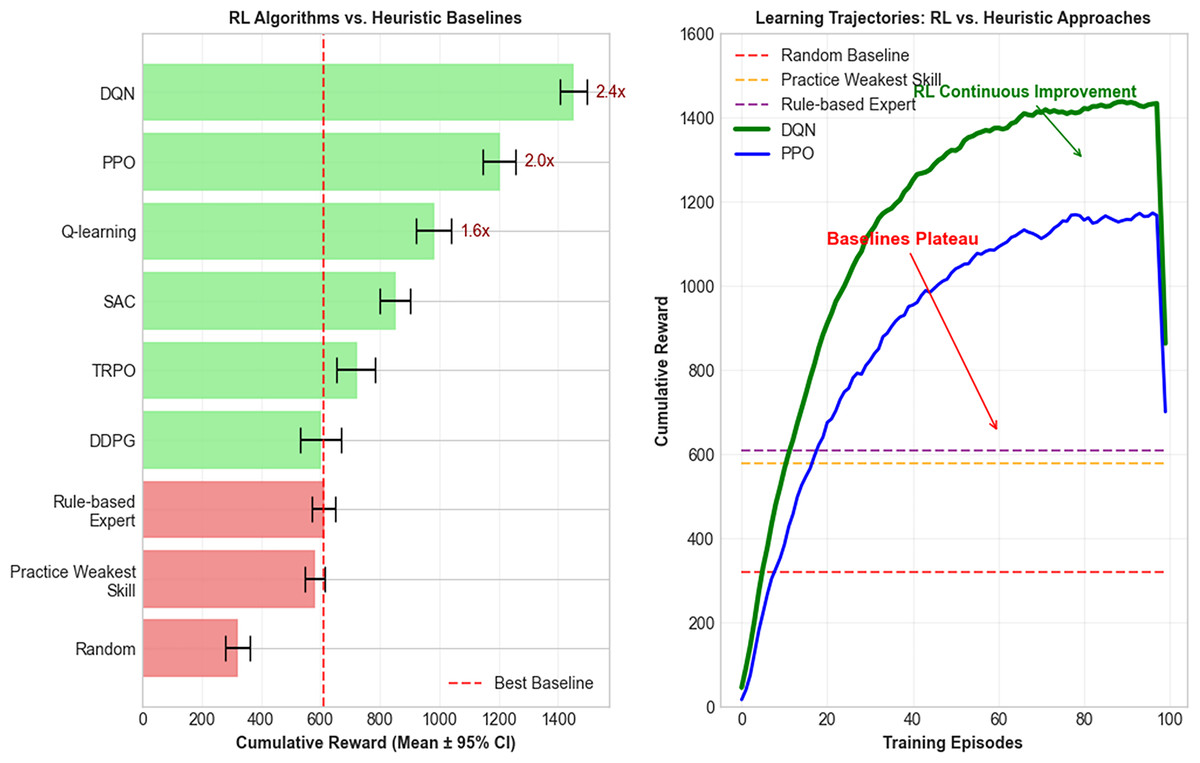
Figure 16: Comparative analysis of salinity baseline methods.
Discussion and analysis
The introduction of an RL based evaluation framework in music education extend the capabilities of current models by offering an adaptive, data-driven, and real-time evaluation. In contrast to traditional systems (i.e., fixed mechanisms of feedback or rule-based tests designed to be both static and unchanging), the proposed model learns over time based on performance data and adapts instructional tasks. Existing work applied Q-learning, PPO, or DDPG on general education tasks and were not very finely adaptive or domain-specific to the demands of skills-based fields such as music. As an illustration, previous studies based on PPO shown moderate levels of feedback personalization without considering changes in skills over time. Conversely, our DQN model does not only have better precision and engagement scores but capturing less Reward Volatility Index (0.17) and higher Engagement Stability Index (0.91) than TRPO (0.28) and DDPG (0.31). Additionally, in contrast to systems operating on pre-determined levels of difficulty, proposed method suggests custom tasks (e.g., sight-reading, rhythmical exercises, expressiveness improvement) depending on the immediate student performance, which make it more context-dependent and personalized.
Implication of the proposed framework
The analysis of the study shows some of the major implications of personalized music education. First, it offers a smart feedback system where a student can get feedback based on his or her skill progression and has intrinsic motivation. Secondly, the framework equips educators with the scalable tool that allows them to track the progress of their students, clarify areas of weaknesses and adjust or accelerate the pacing of a lesson or its content. Pedagogically, the research promotes a move to abandon a one-size-fits-all situation to an individually constructed learning path marked by a data-based direction. On the administrative level, educational establishments can utilize this model in order to introduce more balanced, universally consistent, and flexible assessment procedures. The application of an RL algorithm in the context of gamified music education also indicates the universality of the methods used in domains involving performance-related skills that can establish a new bar of applying AI in the field of personalized education.
Limitations of the proposed framework
The proposed model shows a high accuracy and efficiency in designing of a personalized music education for students. However, there are several limitations. First, lack of generalizability can be presented by the treatment of a simulated dataset since the variables that represent emotional states or social factors are difficult to capture in reality. Second, DQN algorithm has not been tested in unstructured classroom settings; in absence of appropriate calibration, there is a possibility that the algorithm may not perform well. Third, the framework represents four key dimensions of skill (TP, IS, SR and ME), but it is not able to explain such non-quantifiable aspects as creativity or musical intuition. In addition, school environments have hardware and computing limitations that can render deployment impractical. Finally, teacher acceptance and training needs are required for large-scale implementation which need specific efforts on the part of an institution.
Future work
The evaluation of the proposed framework using simulated dataset depicts that in future it can be implemented in a real-life environment (i.e., music academies or conservatories) to check its long-term effects and viability in terms of implementation. The flexibility of the framework will be touched upon by extensions into nearby creative disciplines such as the instruction of dance and art. Also, the incorporation of innovative technology such as VR and AR can provide more visceral feedback and real-life learning. Some of the features based on student emotional feedback and social interaction analytics will also be involved in newer versions to improve the personalization layer further. Another route is at the level of curriculum, where the system facilitates the design of lesson plans in a co-design manner with a constant performance data. Lastly, it will require special teacher training packages and policy-oriented recommendations to facilitate implementation of this AI-based assessment tool in a meaningful way.
Conclusion
This study presents a RL based evaluation system based on the DQN to individualize the education and aims to reduce the limitations of classic subjective evaluations. Using a procedure in which the feedback is based on real time data, the system recorded the performance of students and highlight required skill measurements such as technical proficiency, expressiveness of performance, sight-reading and interpretive skills in a dynamic fashion to aid individual learning. The evaluation agent effectively chooses the best practices of using rewards and penalties in order to enhance learning through a reward punishment mechanism. In 100 episodes of experiments, it was revealed that the proposed model showed improved performance when compared to the baseline RL methods, such as PPO, DDPG, SAC, TRPO, and Q-learning, in the aspect of the cumulative reward, precision, and stability. In simulation study, the DQN model indicated potential improvements in skill development and responsiveness of the feedback system, specifically, DQN achieved up to 25% higher cumulative reward than PPO and 45% higher than DDPG which indicate more efficient task selection. It also achieved the lowest RVI (0.17) and the highest ESI (0.91), suggesting smoother learning trajectories and stronger learner engagement in simulation. The implications of these simulated results indicate that RL has capability to streamline the assessment operations, especially in skill-based fields such as in music education. Therefore, our findings should be interpreted as a promising step rather than a confirmed solution. However, a few knowledge gaps still exist, an insufficient use of gamification-specific measures (e.g., reward volatility, engagement stability) to evaluate the performance of algorithms, and a shortage of classroom-interactable, scalable RL models capable of supporting a diverse set of learner profiles. Beyond simulation, scalability should be validated in real-life classrooms and across various academic subjects. Another area to explore is to make RL models less opaque and obscure to educators in order to guarantee educational acceptability and feasibility. Additionally, it will also investigate the use of hybrid versions of the framework such as Transformer-RL integrations, the use of virtual reality, the use of augmented reality and real world classroom implementations to confirm scalability and a wider applicability of the framework.
Supplemental Information
Supplementary materials.
1. Dataset. 2. Description of the model. 3. Simulation code.