
New hybrid multi-objective feature selection: Boruta-XGBoost
- Published
- Accepted
- Received
- Academic Editor
- Alexander Bolshoy
- Subject Areas
- Artificial Intelligence, Data Mining and Machine Learning, Data Science, Optimization Theory and Computation, Neural Networks
- Keywords
- Artificial neural network, Body fat prediction, Data processing, Feature selection, Machine learning, Boruta-XGBoost hybrid approach, Optimization, Random forest
- Copyright
- © 2026 Yousefi and Varlıklar
- Licence
- This is an open access article distributed under the terms of the Creative Commons Attribution License, which permits unrestricted use, distribution, reproduction and adaptation in any medium and for any purpose provided that it is properly attributed. For attribution, the original author(s), title, publication source (PeerJ Computer Science) and either DOI or URL of the article must be cited.
- Cite this article
- 2026. New hybrid multi-objective feature selection: Boruta-XGBoost. PeerJ Computer Science 12:e3463 https://doi.org/10.7717/peerj-cs.3463
Abstract
In the era of data-intensive science, feature selection has become a cornerstone of building robust machine learning models, particularly in biomedical fields where datasets are often high-dimensional. The process of identifying a subset of relevant and non-redundant features is not merely a means of reducing computational overhead; it is crucial for enhancing model accuracy, preventing overfitting, and improving the interpretability of results. Despite its importance, finding an optimal feature subset remains a significant challenge. This study introduces and validates a novel two-stage hybrid framework, named Boruta-XGBoost (Boruta-Extreme Gradient Boosting), designed to synergize feature selection and prediction. We demonstrate the efficacy of this framework on the complex task of estimating body fat percentage, a problem characterized by correlated anatomical predictors. Our primary goal is to benchmark its performance against a comprehensive suite of established machine learning algorithms. Our proposed framework unfolds in two distinct stages. Initially, we leverage the Boruta algorithm—a powerful wrapper method based on Random Forest—to systematically identify all statistically relevant features. This step ensures that no potentially important variables, including those with subtle interaction effects, are prematurely discarded. Subsequently, an Extreme Gradient Boosting (XGBoost) model is trained exclusively on this refined feature subset. To establish a robust benchmark, we evaluated 16 other models (six linear and 10 non-linear) using the complete feature set. All models were assessed via a 70/30 train-test split and validated using 10-fold cross-validation, with the coefficient of determination (R2) and Root Mean Square Error (RMSE) serving as the primary performance metrics. When trained on the full set of features, the best-performing conventional model—non-linear support vector regression—yielded an R2 of 0.77. In striking contrast, our Boruta-XGBoost framework achieved a markedly superior R2 of 0.88 and a correspondingly lower RMSE. A key finding is that this enhanced predictive accuracy was accomplished using just six features (representing only 46% of the original 13), which were autonomously identified by the Boruta stage.
Conclusion
Our results compellingly demonstrate that the proposed Boruta-XGBoost hybrid framework offers a substantial improvement over conventional modeling approaches. By intelligently decoupling feature selection from prediction, our method constructs a more parsimonious and powerful model. This two-stage strategy underscores the value of integrating rigorous statistical feature filtering with state-of-the-art predictive algorithms, presenting a potent and generalizable approach for tackling complex prediction problems.
Introduction
In the contemporary world, the dimensionality of data is consistently on the rise. A prominent instance of this trend can be observed in the realm of bioinformatics, where data is experiencing substantial growth (Tarczy-Hornoch & Minie, 2005). The increasing number of features in datasets across various fields presents notable challenges for machine learning models. High-dimensional data often includes irrelevant or redundant attributes, which can raise computational costs, hinder model interpretability, and increase the risk of overfitting. For instance, the body fat dataset used in this study contains numerous anthropometric and body composition measurements, yet not all of them equally influence the prediction of body fat percentage. This situation underscores the importance of robust feature selection techniques that can pinpoint the most informative variables, streamline the dataset, and enhance both prediction accuracy and computational efficiency. Moreover, many machine learning applications, including text mining, computer vision, and biomedicine, have witnessed a significant surge in data volume and dimensionality in recent times (Miao & Niu, 2016). Consequently, data mining assumes a vital role in uncovering concealed insights from vast datasets (Jain & Chandrasekaran, 1982).
The dataset can be characterized by two key dimensions: the number of features and the number of samples . It is possible for both and to reach considerable magnitudes. However, such large dataset sizes can give rise to significant challenges within various data mining systems (Liu & Motoda, 2012). To address these challenges, the utilization of “Dimensional Reduction” techniques becomes imperative, forming an integral part of the data pre-processing stage (Tsai & Chou, 2011). Consequently, it holds great importance to reduce the dataset size, particularly when dealing with extensive or multidimensional data (Sugiyama, 2015). In this context, feature selection emerges as a valuable approach for tackling the issues associated with size reduction (Liu & Motoda, 2012).
Feature selection is an essential technique in data pre-processing that plays a crucial role in machine learning (Kalousis, Prados & Hilario, 2007). As research in data mining increases, there is a growing focus on feature selection (Mlambo, Cheruiyot & Kimwele, 2016). This method effectively reduces the dimensionality of data, decreases computational costs, and improves classification performance (Hua, Tembe & Dougherty, 2009). In data mining, feature selection is a fundamental step that enhances algorithm performance by reducing the size of the dataset. However, feature selection algorithms alone may not achieve the optimal solution due to their limited search capabilities (Yusta, 2009). While heuristic methods often provide satisfactory solutions, they may not be suitable for complex problems and heavily rely on the expertise of the developer (Chinneck, 2006; Coello, 2007). On the other hand, metaheuristic algorithms, which utilize randomization and local search techniques, generally outperform simple heuristics (Yang, 2010). Metaheuristics have become the preferred approach due to their ability to comprehensively explore and solve complex problems (Glover & Kochenberger, 2006). Consequently, metaheuristic methods offer a promising solution for accurately addressing feature selection problems.
As mentioned before, feature selection is a crucial step in data preprocessing, allowing for the reduction of data dimensions and improvement in prediction performance. However, traditional methods of feature selection fall short of providing suitable solutions. To address this limitation, we propose a hybrid approach in this article. In our study, we initially performed all data preprocessing steps, excluding feature selection, on the body fat dataset using 16 machine learning algorithms. To address the persistent challenges in feature selection, this article introduces a novel two-stage hybrid framework, termed Boruta-XGBoost. The motivation for this framework stems from a critical gap in many machine learning pipelines: while powerful predictive algorithms like Extreme Gradient Boosting (XGBoost) exist, their performance can be significantly hampered by noisy, redundant, or irrelevant features. Conversely, robust feature selection methods like Boruta excel at identifying statistically relevant variables but are not prediction models themselves.
The novelty of our work, therefore, lies not in inventing new algorithms, but in the synergistic integration of these two powerful components into a structured, two-stage pipeline. We propose a strategic decoupling of the feature selection and prediction tasks. By first employing Boruta to meticulously curate a clean and highly relevant feature subset, we then empower the XGBoost model to learn from an optimized input, thereby unlocking its full predictive potential.
The main contributions of this article are thus three-fold and can be summarized as follows:
-
(1)
Methodological design: We present a well-defined hybrid framework that combines a wrapper-based statistical feature selection method with a state-of-the-art prediction model. This provides a robust and generalizable template for tackling complex prediction tasks in high-dimensional spaces.
-
(2)
Empirical validation: We provide compelling empirical evidence of the framework’s superiority. Through a case study on body fat percentage prediction, we demonstrate that the Boruta-XGBoost approach achieves a significantly higher predictive accuracy (R2 = 0.88) than 16 baseline models, including a standard XGBoost model trained on all features.
-
(3)
Enhanced efficiency and interpretability: We show that this superior performance is achieved using a more parsimonious model, which relies on only 46% of the original features. This not only improves the computational efficiency of the prediction stage but also enhances model interpretability by focusing on the most critical predictive factors.
This study thus validates the effectiveness of our hybrid approach and highlights a powerful strategy for building more accurate and reliable machine learning models.
The article is organized as follows: ‘Related Works’, related works on feature selection methods are discussed. ‘Proposed Method’, a comprehensive description of the materials and methods employed is provided, including an in-depth explanation of the proposed Boruta-XGBoost Hybrid Approach for intelligent feature selection. ‘Results and Discussion’ is dedicated to presenting the obtained results and conducting comparisons between the performance of 16 machine learning methods and the proposed A Boruta-XGBoost Hybrid Approach. Lastly, the article concludes with a section encompassing the key findings, conclusions, and research perspectives for future endeavors.
Related works
The increasing complexity and dimensionality of modern datasets present significant challenges for machine learning models. High-dimensional data often contain irrelevant or redundant features that can adversely affect predictive performance, increase computational cost, and hinder model interpretability. Feature selection (FS) has emerged as a fundamental preprocessing step, aiming to retain only the most informative features while eliminating redundant or irrelevant ones. By reducing dimensionality, FS improves interpretability, enhances generalization, and reduces computational burden, thereby supporting more robust and efficient learning across diverse domains (Theng & Bhoyar, 2024).
Over the past decades, numerous FS methods have been developed, reflecting a wide spectrum of strategies and objectives. These methods vary in terms of search mechanisms, evaluation metrics, and integration with learning algorithms. Traditional filter approaches evaluate features independently based on statistical or information-theoretic criteria, offering computational efficiency but often lacking direct consideration of model performance. Wrapper methods, by contrast, assess feature subsets using a predictive model, ensuring higher accuracy at the cost of increased computational complexity. Hybrid methods combine the advantages of both, balancing efficiency and performance. Selecting an appropriate method, however, remains highly context-dependent, requiring careful consideration of dataset size, structure, and the relationship between features and target variables.
In recent years, research has increasingly framed FS as a multi-objective optimization problem, aiming to simultaneously maximize predictive accuracy while minimizing the number of selected features. Metaheuristic and evolutionary algorithms have become popular tools in this context, with numerous hybrid approaches demonstrating strong performance. For instance, combinations of Harris Hawks Optimization with Fruit Fly Optimization (MOHHOFOA) have shown competitive results on benchmark datasets, while hybrid methods integrating Particle Swarm Optimization (PSO) and Gray Wolf Optimization (GWO) have proven effective for high-dimensional gene expression data (Abdollahzadeh & Gharehchopogh, 2022; Dhal & Azad, 2021).
Multi-objective particle swarm optimization (MOPSO) has also been applied to cost-sensitive FS, producing Pareto fronts that balance accuracy and cost. This approach incorporates evolutionary operators, crowding distance, and archive management to maintain solution diversity (Zhang, Gong & Cheng, 2015). Further developments include the integration of multi-task learning into multi-objective FS frameworks, which accelerates convergence and improves solution diversity by transferring knowledge from auxiliary single-objective tasks (Liang et al., 2023).
The synergy between filter-based methods and evolutionary optimization has attracted attention as well. Filter-based rankings can initialize populations in evolutionary algorithms, improving convergence speed and solution diversity. Examples include the Hybrid Filter-based Multi-Objective Evolutionary Algorithm (HFMOEA) and self-learning binary differential evolution strategies, which demonstrate robust feature subset selection and strong generalization (Kundu & Mallipeddi, 2022; Zhang et al., 2020). Large-scale multi-objective FS algorithms with real-valued encodings further highlight ongoing methodological innovations in the field (Fu et al., 2024).
Domain-specific applications have validated the effectiveness of advanced FS methods. In renewable energy forecasting, Lv & Wang (2023) proposed a hybrid framework combining FWNSDEC (a hybrid filter-wrapper non-dominated sorting differential evolution with K-medoid clustering) with deep learning models such as ConvLSTM. Singular Spectrum Analysis (SSA) decomposes time series data to extract meaningful patterns, which are then fed into spatiotemporal models. This approach significantly outperformed benchmark models on four real-world datasets from NREL, achieving MAPE values as low as 1.42% for one-step forecasting (Lv & Wang, 2023).
In the domain of software defect prediction (SDP), feature relevance is critical to model performance. Ni et al. (2019) introduced MOFES, a multi-objective FS framework using NSGA-II to minimize feature count while maximizing predictive accuracy. Across multiple benchmark datasets, MOFES consistently selected compact and informative feature subsets, improving model performance and providing stable results across runs (Ni et al., 2019). Similarly, hybrid GA-Pearson correlation approaches have been shown to produce compact, high-quality feature subsets, effectively outperforming conventional methods (Saidi, Bouaguel & Essoussi, 2018; Xue et al., 2021).
Additional studies have extended the multi-objective FS paradigm to include reliability alongside accuracy and subset size. NSGA-III has been applied to select feature subsets that are accurate, compact, and robust to missing values, offering balanced performance in incomplete datasets (Xue et al., 2021). GADMS combined with the Ideal Point Method (IPM) has been used for industrial datasets to identify key quality characteristics (KQCs) from imbalanced production data, demonstrating superior performance over enhanced NSGA-II and MOPSO variants (Li, Xue & Zhang, 2020).
While the literature is rich with advanced multi-objective and meta-heuristic approaches, many of these methods can be complex to implement and tune. Our study takes a different but complementary path. We propose a pragmatic and powerful two-stage framework that combines a statistically-grounded wrapper method (Boruta) with a state-of-the-art predictive model (XGBoost). The aim is to provide an effective, interpretable, and robust solution that leverages the strengths of both statistical rigor and high-performance machine learning, offering a valuable alternative to the purely optimization-driven approaches. A summary of representative feature selection methods, their optimization objectives, strengths, and limitations is provided in Table 1.
| Method | Optimization objective | Approach | Strengths | Limitations |
|---|---|---|---|---|
| MOHHOFOA (Abdollahzadeh & Gharehchopogh, 2022) | Max accuracy, min features | Hybrid metaheuristic (HHO + FOA) | Compact subsets, strong convergence, robust across benchmarks | High computational cost, parameter tuning required |
| PSO-GWO Hybrid (Dhal & Azad, 2021) | Max accuracy, min features | Two-phase metaheuristic | Effective for high-dimensional data, balances exploration/exploitation | Complex design, sensitive to initialization |
| MOPSO (Cost-Based) (Zhang, Gong & Cheng, 2015) | Max accuracy, min cost | Multi-objective PSO | Flexible trade-offs, high-quality Pareto fronts | May require multiple runs for stability |
| HFMOEA (Kundu & Mallipeddi, 2022) | Max accuracy, min features | Filter-initialized NSGA-II | Fast convergence, diverse non-dominated solutions | Filter-based initialization may introduce bias |
| MOFS-BDE (Zhang et al., 2020) | Max accuracy, min features | Binary Differential Evolution + Self-learning | Balances local and global search, competitive solution quality | Implementation complexity, parameter-sensitive |
| Large-scale MOFS (Fu et al., 2024) | Max accuracy, min features | Real-valued multi-objective FS | Scalable, high-quality diverse solutions | High computational cost |
| FWNSDEC + ConvLSTM (Lv & Wang, 2023) | Max forecast accuracy | Hybrid FS + deep learning | Captures spatiotemporal patterns, strong predictive performance | Domain-specific, high computational demand |
| MOFES (SDP) (Ni et al., 2019) | Max accuracy, min features | NSGA-II based multi-objective | Consistent feature selection, compact subsets, interpretable | Limited exploration in complex datasets |
| Hybrid GA + PCC (Saidi, Bouaguel & Essoussi, 2018) | Max accuracy, min features | GA + Correlation-based evaluation | Compact and informative feature subsets | Computationally intensive, sensitive to GA parameters |
| NSGA-III (Three-objective FS) (Xue et al., 2021) | Max accuracy, min features, max reliability | Multi-objective EA | Robust to missing data, accurate and compact | Computationally intensive |
| GADMS + IPM (Li, Xue & Zhang, 2020) | Max subset importance, min size | GA + DMS + Ideal Point Method | Effective for imbalanced industrial datasets, accurate KQC selection | Two-phase process, computational cost |
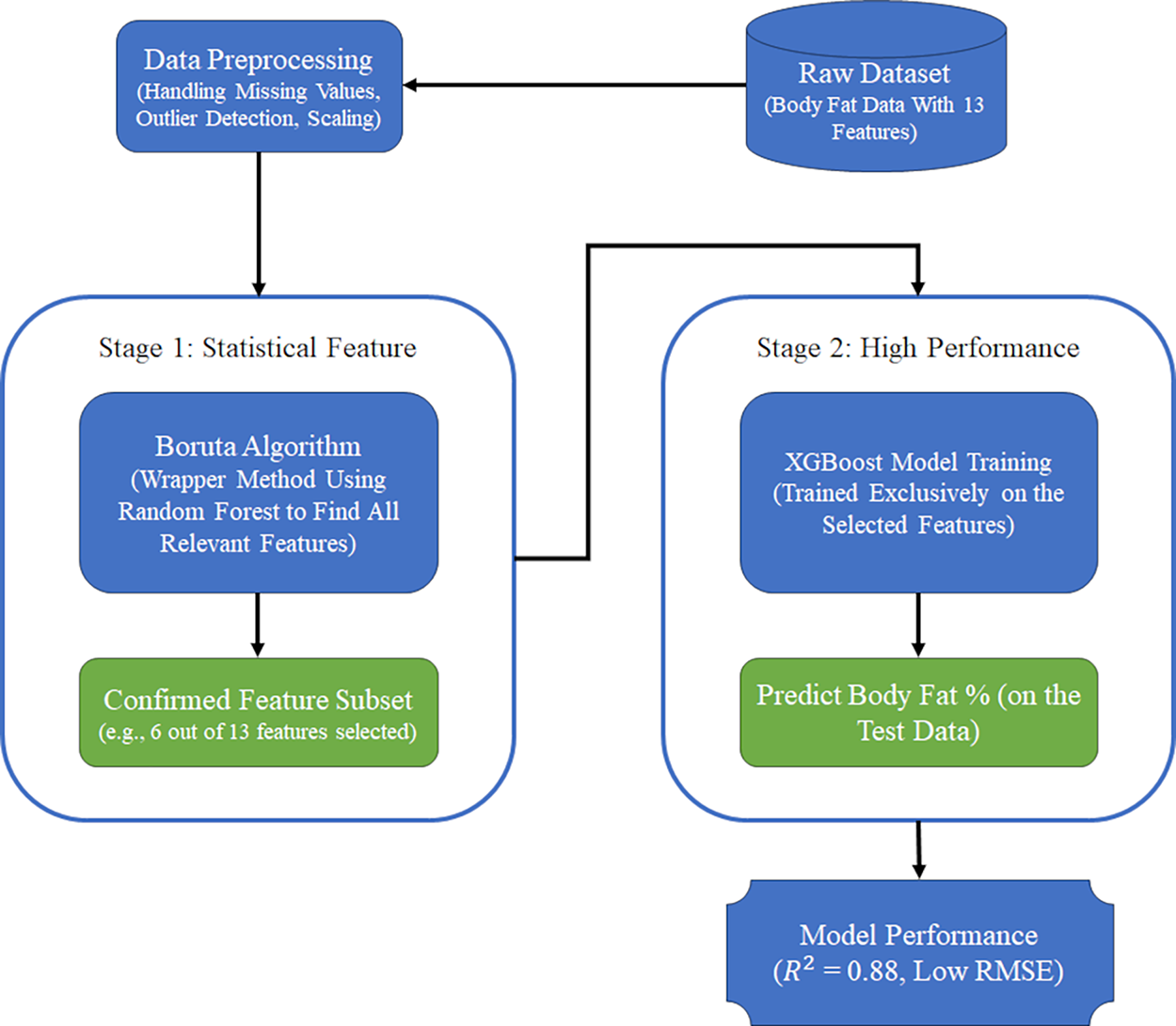
Proposed method
The flowchart of the proposed method is shown in Fig. 1.
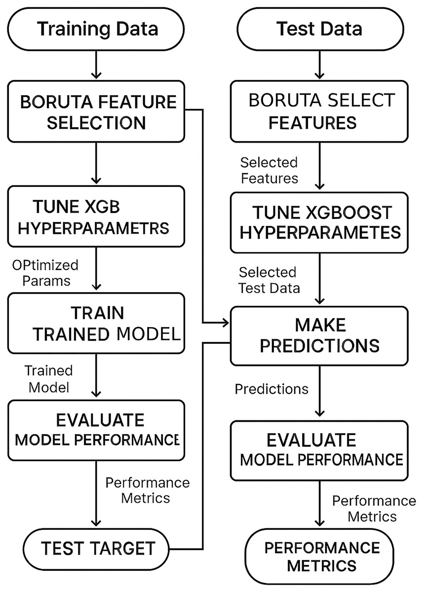
Figure 1: The flowchart of the proposed method.
Dataset
In this section, the authors begin by introducing the dataset used in the study. The steps involved in the processes described in this article are then explained in a sequential manner to facilitate the readers’ understanding. The dataset (Johnson, 1996) used in this article focuses on predicting body fat percentage using anatomical measurements. It consists of data from 252 individuals, with 13 physical characteristics measured for each person. The specific names of these features are listed in Table 2.
| Number of features | Unit of measurement |
|---|---|
| Age | Years |
| Weight | Pound |
| Height | Inches |
| Neck circumference | Centimeter |
| Chest circumference | Centimeter |
| Abdomen circumference | Centimeter |
| Hip circumference | Centimeter |
| Thigh circumference | Centimeter |
| Knee circumference | Centimeter |
| Ankle circumference | Centimeter |
| Biceps circumference | Centimeter |
| Forearm circumference | Centimeter |
| Wrist circumference | Centimeter |
General information about dataset
In this section, our aim is to obtain general information about the dataset. To achieve this, we perform several calculations for each feature, including count, mean, standard deviation, minimum, maximum, and quartile values (0%, 5%, 50%, 95%, 99%, 100%). These calculations provide us with an overview of the dataset and its characteristics.
As observed in Table 3 and Fig. 2, the features Weight, Height, Nip, and Ankle exhibit outlier values, resulting in a significant difference between the 99% and 100% quartile values. This discrepancy has an impact on our model and hinders the attainment of desirable results. In the upcoming section, we will address this issue and discuss methods to handle outlier data effectively.
| Count | Mean | Std | Min | 0% | 5% | 50% | 95% | 99% | 100% | Max | |
|---|---|---|---|---|---|---|---|---|---|---|---|
| Body fat | 252 | 19.15 | 8.37 | 0 | 0 | 6.055 | 19.2 | 32.6 | 36.621 | 47.5 | 47.5 |
| Age | 252 | 44.88 | 12.60 | 22 | 22 | 25 | 43 | 67 | 72 | 81 | 81 |
| Weight | 252 | 81.16 | 13.33 | 53.75 | 53.75 | 61.86 | 80.06 | 102.35 | 111.46 | 164.72 | 164.72 |
| Height | 252 | 178.18 | 9.30 | 74.93 | 74.93 | 167.35 | 177.80 | 189.23 | 193.04 | 197.49 | 197.49 |
| Neck | 252 | 37.99 | 2.43 | 31.1 | 31.1 | 34.255 | 38 | 41.845 | 42.996 | 51.2 | 51.2 |
| Chest | 252 | 100.82 | 8.43 | 79.3 | 79.3 | 89.02 | 99.65 | 116.34 | 120.73 | 136.2 | 136.2 |
| Abdomen | 252 | 92.56 | 10.78 | 69.4 | 69.4 | 76.875 | 90.95 | 110.76 | 120.01 | 148.1 | 148.1 |
| Hip | 252 | 99.90 | 7.16 | 85 | 85 | 89.155 | 99.3 | 112.13 | 115.79 | 147.7 | 147.7 |
| Thigh | 252 | 59.41 | 5.25 | 47.2 | 47.2 | 51.155 | 59 | 68.545 | 72.696 | 87.3 | 87.3 |
| Knee | 252 | 38.59 | 2.41 | 33 | 33 | 34.8 | 38.5 | 42.645 | 44.592 | 49.1 | 49.1 |
| Ankle | 252 | 23.10 | 1.69 | 19.1 | 19.1 | 21 | 22.8 | 25.445 | 28.274 | 33.9 | 33.9 |
| Biceps | 252 | 32.27 | 3.02 | 24.8 | 24.8 | 27.61 | 32.05 | 37.2 | 38.5 | 45 | 45 |
| Forearm | 252 | 28.66 | 2.02 | 21 | 21 | 25.7 | 28.7 | 31.745 | 33.394 | 34.9 | 34.9 |
| Wrist | 252 | 18.23 | 0.93 | 15.8 | 15.8 | 16.8 | 18.3 | 19.8 | 20.645 | 21.4 | 21.4 |
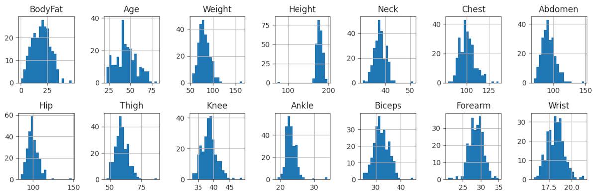
Figure 2: Histogram of body fat dataset.
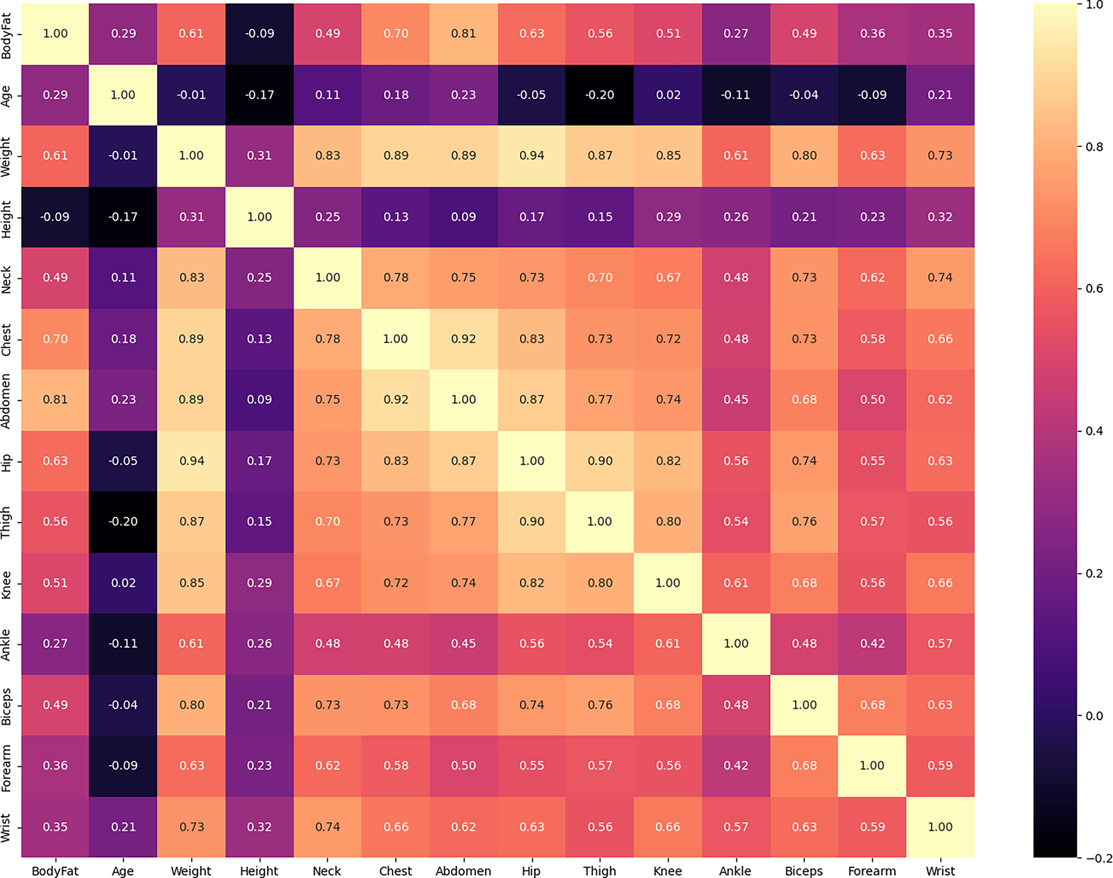
In the subsequent step, our aim is to assess the strength of the relationship between variables in the dataset, a measure known as correlation. Through the analysis of the correlation matrix, we can determine which features exhibit a high degree of similarity.
To better understand the data distribution, we first visualized the target variable. Figure 3 presents a histogram of the body fat percentage, which shows a roughly unimodal and approximately symmetric distribution.

Figure 3: Distribution of body fat percentage.
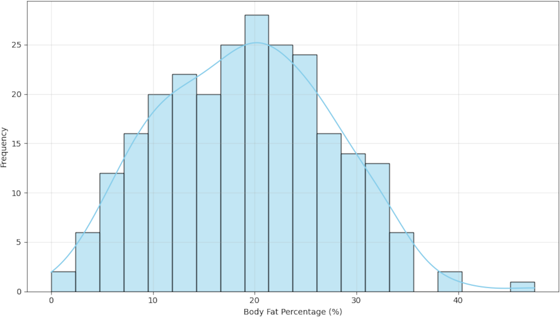
The presence of these potential outliers is visualized in Fig. 4, which presents box plots for each of the predictor variables. As illustrated, features such as Weight, Height, and Ankle exhibit data points beyond the typical range (1.5 times the interquartile range).
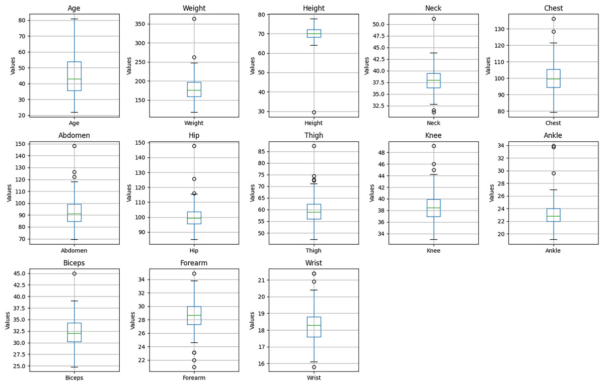
Figure 4: Boxplots of predictor variables.
As depicted in Fig. 5, certain variables display a stronger positive correlation with each other. For instance, the Hip variable demonstrates this relationship. To enhance the speed and efficiency of our model, and to understand multicollinearity, we note variables that exhibit stronger positive correlations, although the Boruta method is generally robust to multicollinearity.
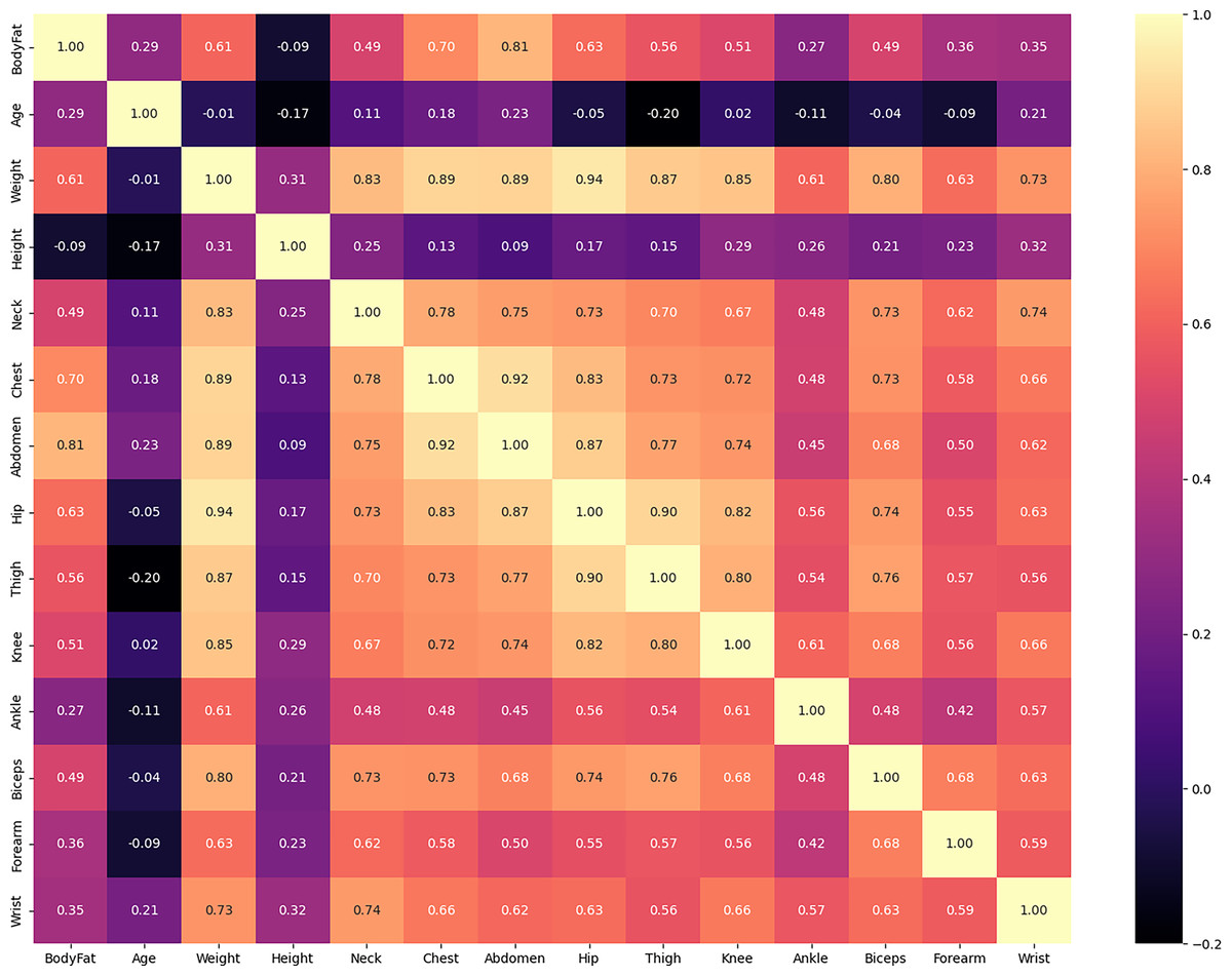
Figure 5: Correlation matrix between features of body fat dataset.
In the final step, we employ the joint plot method to gain a deeper understanding of the relationship between variables, as well as the individual distribution of each variable. This method facilitates a clearer comprehension of the association between independent and dependent variables, aiding us in selecting more significant features.
As depicted in Fig. 6, the joint diagram is comprised of three distinct sections. The central portion presents insights into the relationship between the independent and dependent variables, providing information regarding the joint distribution. The remaining two sections represent the marginal distributions for the dependent and independent variable axes.
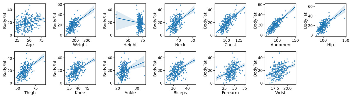
Figure 6: The joint plot of the body fat dataset.
Data pre-processing
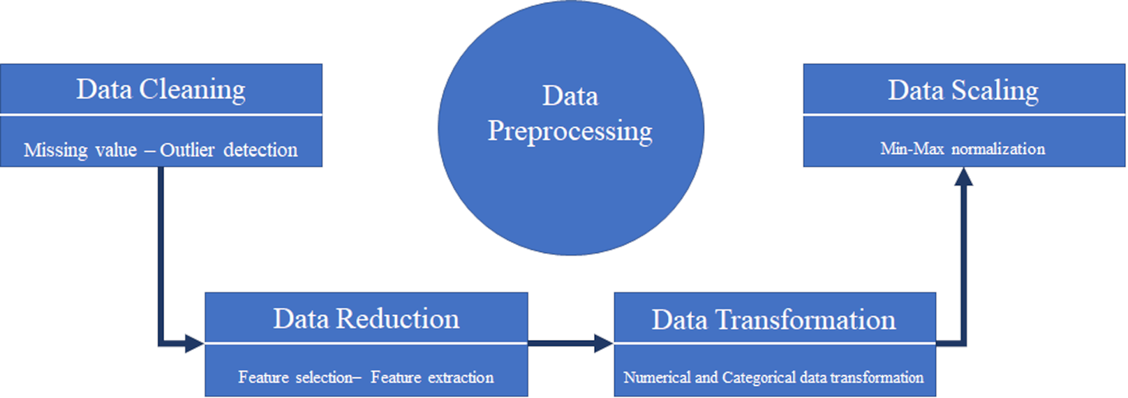
Data mining refers to the process of extracting valuable patterns and models from a dataset. However, the quality of the data is crucial in uncovering these patterns. Raw and unprocessed data often contain empty, noisy, incomplete, inconsistent, and outlier values. Therefore, effective data pre-processing is necessary before conducting data mining to extract useful models from the dataset. Data pre-processing, which involves preparing the data before extracting information and models, plays a vital role in the accuracy and effectiveness of the resulting models (Zhang, Zhang & Yang, 2003). In this article, we will begin by performing the data pre-processing stage prior to any model or information extraction. Figure 7, illustrates the sequential workflow used to prepare the dataset for analysis. The stages include:
-
a.
Data cleaning: Handling inconsistencies such as missing values and outliers to ensure data quality.
-
b.
Data reduction: Employing feature selection techniques (in our case, Boruta) to reduce the dimensionality of the dataset by identifying the most relevant variables.
-
c.
Data transformation: Converting data into a suitable format for modeling, although this step was minimal in our study as features were primarily numerical.
-
d.
Data scaling: Normalizing the range of feature values (e.g., using Min-Max scaling) to ensure that all features contribute equally to model training, particularly for distance-based algorithms.
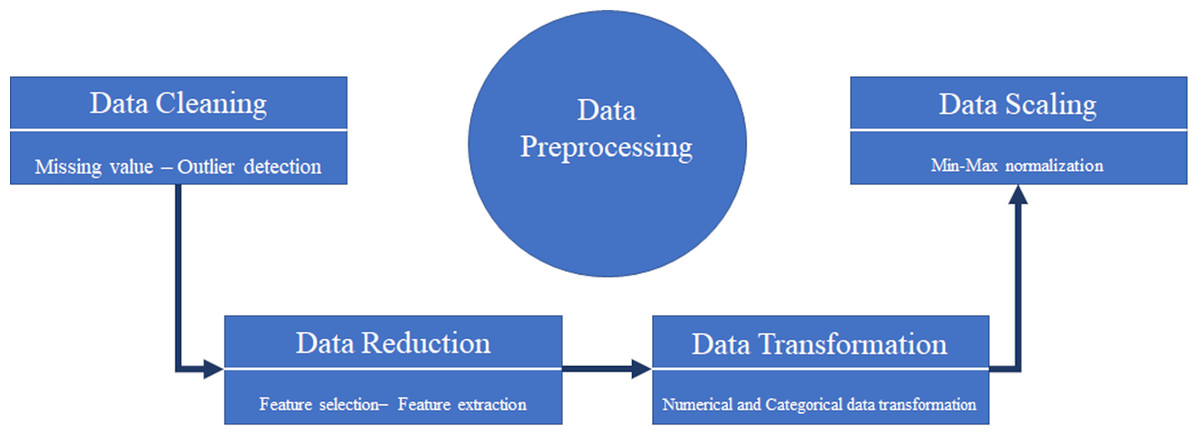
Figure 7: Typical data pre-processing tasks.
Data cleaning
Raw data often contains defects, noise, and outliers, which need to be addressed before further analysis. Data cleaning, the initial step in data pre-processing, aims to handle these issues. It is crucial to perform effective data cleaning to avoid the creation of inefficient models that deviate from our objectives. Therefore, data cleaning holds significant importance in the data pre-processing pipeline (García, Luengo & Herrera, 2015; Maingi, 2015). As depicted in Fig. 7, this article will commence with data cleaning as the first step. Data cleaning is further divided into two parts: missing value handling and outlier detection.
A missing value refers to data that is typically not measured or left blank during data collection. It is generally recommended to handle missing values rather than ignoring or deleting them, but it is important to impute missing values in a reasonable manner. Several solutions exist to address missing data, with common approaches including the use of averages, medians, and machine learning algorithms for imputation (García, Luengo & Herrera, 2015; Luengo, García & Herrera, 2012). Note that XGBoost can handle missing values internally, but imputation might still be performed.
Outlier data lacks a precise and universally accepted definition in the literature (Ayadi et al., 2017). However, it can be described as data points or intervals that deviate significantly from the rest of the dataset. The presence of outliers in the dataset can adversely affect model performance and lead to misleading results (Wang, Bah & Hammad, 2019).
Various methods can be employed to handle outlier data, and in this article, we will utilize the quartile method. This method involves determining the first quartile ( ) and third quartile ( ) of the data. By checking if the data falls outside the range of and , outliers can be identified and adjusted accordingly (Gustavsen et al., 2011).
Data reduction
Data reduction refers to the process of reducing certain aspects of data. It can involve reducing the data’s count or dimensions, resulting in a smaller data volume. The goal of data reduction can vary, ranging from removing invalid data to generating statistical and summary data for various applications (García, Luengo & Herrera, 2015).
Data reduction is commonly carried out using row and column methods. The row method focuses on reducing the data sample through techniques like random and stratified sampling (Fan et al., 2015). On the other hand, the column method aims to reduce the number of variables in the dataset. There are typically three approaches for the column method. The first involves using domain knowledge for variable selection. The second approach is feature selection, which identifies the most important features (Liu & Motoda, 1998, 2007). The third approach is feature extraction, which creates new features from existing ones (Fan et al., 2021; Liu & Motoda, 1998). In this article, we will focus on the feature selection method since our primary objective is to intelligently select important and useful features from the body fat dataset using the Boruta algorithm, followed by prediction using XGBoost.
Feature selection is a crucial step in data mining that focuses on selecting relevant features from a dataset. It plays a role in separating relevant features from irrelevant ones, especially in high-dimensional data (Ramchandran & Sangaiah, 2018). Additionally, feature selection serves as a dimensionality reduction technique, enhancing classification accuracy by removing irrelevant or unnecessary features (Dey et al., 2018). The feature selection process involves five fundamental steps, As you can see in Fig. 8, and the choices made at each step directly impact the performance of feature selection (Langley, 1994). In the following section, we will briefly outline these steps.
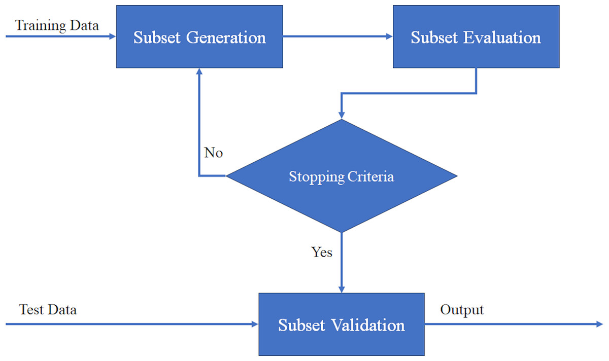
Figure 8: General procedure for feature selection process.
Step 1 involves determining the search direction and starting point for feature selection. The search can begin with an empty set and gradually add features in each iteration, known as forward searching. Alternatively, the search can start with a full set and eliminate features iteratively, known as reverse elimination search. A two-way search strategy involves simultaneously adding and removing features. Another option is to randomly select features to create an initial subset (Ang et al., 2015). Note that Boruta uses an iterative approach based on feature importance comparison.
Step 2 involves determining the search strategy for feature selection. An effective search strategy should include global search capabilities, fast convergence to the optimal solution, efficient local search, and computational efficiency (Gheyas & Smith, 2010). Search strategies can be categorized into three groups: exponential, sequential, and random, as studied by various researchers (Chan et al., 2010; Kumar & Minz, 2014; Muni, Pal & Das, 2006; Ruiz, Riquelme & Aguilar-Ruiz, 2005).
Step 3 involves determining the evaluation criteria for assessing the effectiveness of different feature selection techniques. Evaluation criteria are essential for selecting the most appropriate features. The choice of evaluation criteria depends on the specific problem and data being analyzed. Commonly used evaluation criteria in feature selection include Filter (Chandrashekar & Sahin, 2014), Wrapper (Kohavi & John, 1997), Embedded (Zheng & Casari, 2018), and Ensemble (Opitz & Maclin, 1999). Boruta is a Wrapper method, using Random Forest as the embedded evaluation model.
Step 4 involves determining the stop criteria for the feature selection process. The stop criteria determine when the process will terminate. An appropriate stop criterion helps avoid overfitting and reduces computational complexity, leading to a more efficient generation of the optimal feature subset. The choice of stop criteria may be influenced by decisions made in earlier steps. Common features of stopping criteria are given below (Ang et al., 2015; Kumar & Minz, 2014; Liu & Yu, 2005):
A predefined number of features is reached.
A predefined number of iterations is reached. (A common stopping criterion for Boruta, besides stability).
The performance improvement between iterations falls below a threshold.
An optimal feature subset is deemed to be found based on some evaluation function or stability criterion. (Boruta stops when all features are confirmed or rejected, or max iterations are hit).
Step 5 involves validating the final results obtained from the feature selection process. One way to validate the results is by comparing them with prior knowledge of the data, if available. This can be done by comparing the selected features with a known set of relevant features (Liu & Motoda, 1998; Zeng et al., 2009). However, in real-world applications, such prior knowledge is often not available. In such cases, indirect validation methods are used, such as cross-validation, confusion matrix, Jaccard similarity-based measure, and random index. Cross-validation is the most commonly used validation technique (Bolón-Canedo, Sánchez-Maroño & Alonso-Betanzos, 2013).
Feature extraction is a method that goes beyond selecting important features and aims to create new features by combining dataset variables in linear or non-linear ways (Liu & Motoda, 2013). However, in this article, our focus is on selecting useful features rather than creating new ones. Therefore, we did not perform any feature extraction on the variables of the body fat dataset.
Data transformation
Data transformation is an important process in data mining that involves converting numerical data into categorical data and vice versa. The main purpose of data transformation is to make the datasets compatible for use in data mining algorithms. By transforming the data, we can ensure that the algorithms can effectively analyze and extract patterns from the dataset. This process helps to enhance the accuracy and efficiency of the data mining process, leading to more accurate results and insights (Fan et al., 2021). This step is minimal in this study as features are mostly numerical and tree-based methods like RF/XGBoost handle numerical data directly.
Data scaling
Changing the range of data from one range to another is called data scaling. There are many ways to scale the data, but in this article, we used the Min-Max normalization method. Min-Max normalization is a very simple method of data scaling that puts the data in a predefined range and makes sure that the original relationship between the data is always preserved (Fan et al., 2021; Patro & Sahu, 2015). The formula is (Jain, Nandakumar & Ross, 2005). While tree-based algorithms like Random Forest (used in Boruta) and XGBoost are generally insensitive to the scale of the features, scaling can sometimes be beneficial for other parts of the pipeline or numerical stability, and is often performed as a standard preprocessing step.
XGBoost
XGBoost is a powerful and widely adopted machine learning algorithm based on the gradient boosting framework (Chen & Guestrin, 2016). It has gained significant popularity due to its high performance and computational efficiency, particularly in machine learning competitions and industrial applications. XGBoost sequentially trains weak learners (typically decision trees), where each new model attempts to correct the errors made by the previous ensemble. Key features of XGBoost include:
Regularization: XGBoost incorporates L1 (Lasso) and L2 (Ridge) regularization into its objective function to prevent overfitting and produce simpler models.
Handling missing values: XGBoost can intrinsically handle missing values within the data.
Built-in Cross-Validation: The algorithm provides the capability to perform cross-validation at each boosting iteration.
Parallel processing: XGBoost is designed for efficient utilization of multi-core processors and can perform tree construction in parallel.
Tree pruning: It employs both “max depth” constraints and pruning based on negative loss reduction (gamma parameter).
The overall objective function that XGBoost aims to minimize combines the loss function and a regularization term:
where:
is the loss function, a differentiable convex function that measures the difference between the true target value and the prediction for the i-th training sample.
denotes the summation of the loss over all n training samples.
is the regularization term for the k-th tree. This term penalizes the complexity of the model to prevent overfitting. It is typically defined as , where T is the number of leaves, w is the vector of leaf weights, and and are regularization parameters.
denotes the summation of the complexity penalty over all K trees in the ensemble.
represents the k-th decision tree in the model.
represents the set of all parameters to be learned.
Optimization
Optimization is the process of finding the most optimal solution or outcome for a problem by minimizing effort or maximizing gain. It involves determining the conditions that yield the maximum or minimum value of a specific function. By employing mathematical evaluation and modeling the problem as an objective function, optimization aims to search for the best solution among all possible alternatives. This mathematical technique is widely used to solve problems and make informed decisions in various fields (Burke & Kendall, 2005).
As depicted in the following Equation, the standard representation of an optimization problem involves minimizing the objective function (Sengupta, Gupta & Dutta, 2016):
subject to:
where is the function to be optimized, represents inequality constraints, and represents equality constraints. In wrapper feature selection like Boruta, the objective function is implicitly the performance of the underlying machine learning model, evaluated iteratively.
Advanced feature selection algorithms
Throughout history, problem-solving approaches have often been based on intuition or heuristics. This reliance has contributed to the success and popularity of meta-heuristic algorithms among researchers, which mimic natural processes to find acceptable solutions to complex problems through trial and error (Yang, 2010). Beyond meta-heuristics, other advanced techniques like wrapper methods have been developed for feature selection.
Advanced feature selection algorithms, including meta-heuristics and wrapper methods like Boruta, are designed to tackle complex optimization problems that cannot be effectively solved using classical or simpler filter methods. These algorithms are considered highly effective and widely applicable, especially for real-world problems (Dokeroglu, Deniz & Kiziloz, 2022). The main advantage lies in their effectiveness and general applicability. Unlike classical optimization algorithms, these methods focus on the exploration and exploitation of the feature space, often integrating machine learning models directly into the evaluation process. While parameter tuning remains important, they aim to reduce the time and cost associated with finding improved feature subsets compared to exhaustive search (Ólafsson, 2006). The general framework for many search-based algorithms (especially meta-heuristics) is as follows (Almufti, 2019):
-
(1)
Initialization: Initialize a set of candidate solutions (feature subsets) randomly or using a heuristic.
-
(2)
Evaluation: Evaluate the fitness of each candidate solution using an objective function (often involving a learning model).
-
(3)
Iteration: Repeat the following steps until a stopping criterion is met: a. Selection: Select a subset of candidate solutions based on their fitness values. b. Variation: Apply rules or operators to the selected candidates to generate new candidate solutions. c. Evaluation: Evaluate the fitness of the new candidate solutions. d. Update: Update the set of candidate solutions based on the fitness values.
-
(4)
Termination: Stop the algorithm when a stopping criterion is met.
Boruta follows an iterative process based on comparing real vs shadow feature importance.
The Boruta algorithm
Boruta is a wrapper feature selection algorithm designed to identify all statistically relevant features in a dataset concerning a target variable (Kursa & Rudnicki, 2010). The name ‘Boruta’ is derived from a demon in Slavic mythology who dwelled in pine forests; the authors of the algorithm chose this name metaphorically for its function of exploring the forest of features. It is built upon the Random Forest algorithm and utilizes a clever approach to determine feature importance. The core idea of Boruta is to compare the importance of the original features against the importance of randomized, “shadow” features. The main steps of the Boruta algorithm are as follows:
-
(1)
Create shadow features: For each original feature in the dataset, a copy is created, and its values are randomly permuted across the samples. These new features are termed “shadow features.”
-
(2)
Train model: A Random Forest model is trained on the extended dataset containing both original and shadow features.
-
(3)
Calculate importance: Feature importance scores (typically Mean Decrease Accuracy or Mean Decrease Gini) are computed for all features (original and shadow) using the trained Random Forest.
-
(4)
Determine threshold: The maximum importance score among all shadow features (Maximum Z-score Among Shadow Attributes—MZSA) is identified and serves as the importance threshold for that iteration.
-
(5)
Compare and decide: For each original feature, its importance score is compared against the MZSA. A statistical test (usually a binomial test across multiple iterations) is used to assess whether a feature’s importance is significantly higher than the threshold. Based on this comparison, features are classified into three categories:
Confirmed: Features whose importance is consistently and significantly higher than the MZSA.
Rejected: Features whose importance is consistently and significantly lower than or equal to the MZSA.
Tentative: Features whose importance scores are close to the MZSA, making a definitive decision difficult within the current iterations.
-
(6)
Iterate: Rejected features and shadow features are removed from the dataset, and steps 2–5 are repeated until all features are either Confirmed or Rejected, or a predefined maximum number of iterations is reached. Any remaining Tentative features might be resolved by comparing their median importance against the median importance of the shadow features across all runs.
The final output of Boruta is the set of “Confirmed” features, considered relevant to the target variable. This method is known for its ability to identify all relevant features, including those that might be weakly correlated or interact with others.
Feature selection with advanced algorithms
Feature selection is a complex problem, prompting researchers to utilize advanced artificial intelligence and statistical methods. For years, efforts have focused on finding optimal ways to enhance accuracy and efficiency in this scientific domain. Meta-heuristic algorithms and wrapper methods like Boruta are recognized for being more effective than simpler methods in improving feature selection results. Recent studies demonstrate the ability of these algorithms to yield high-accuracy results and refine the feature selection process (Yusta, 2009).
Here are the general steps to perform feature selection using advanced wrapper algorithms like Boruta (followed by prediction with XGBoost):
-
(1)
Define the problem: The objective is to predict body fat percentage using an optimal subset of anatomical features.
-
(2)
Choose the feature selection algorithm: The Boruta algorithm is selected for its capability to find all relevant features.
-
(3)
Execute Boruta: The Boruta algorithm is run on the training dataset. It iteratively compares the importance of real features against shadow features to identify ‘Confirmed’ features.
-
(4)
Select the prediction model: The XGBoost algorithm is chosen as the final prediction model due to its strong performance.
-
(5)
Train the final model: An XGBoost model is trained using only the features identified as ‘Confirmed’ by Boruta on the training data.
-
(6)
Evaluate performance: The performance of the trained XGBoost model is assessed on a separate test dataset using appropriate metrics (e.g., RMSE, R2).
-
(7)
Validate: Techniques like cross-validation (potentially used during XGBoost parameter tuning or for overall evaluation) ensure the robustness and generalizability of the results.
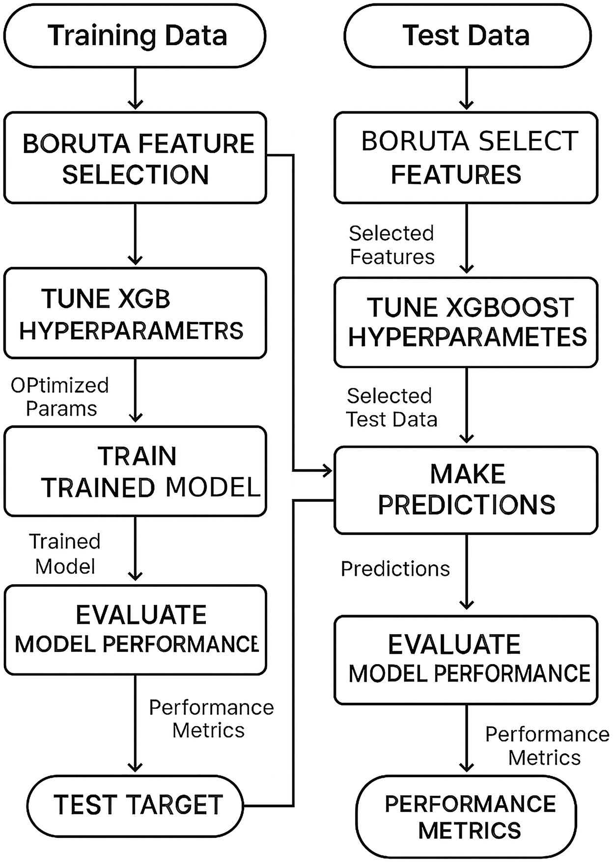
The proposed Bruta-XGBoost hybrid framework
Our proposed method for intelligent feature selection and high-accuracy prediction is a two-stage hybrid framework that sequentially combines the Boruta algorithm and Extreme Gradient Boosting (XGBoost). The core principle of this framework is to first purify the feature space using a statistically robust method before engaging a powerful predictive model. This strategic separation allows each component to perform its specialized task optimally. Figure 9 illustrates the workflow of our framework.
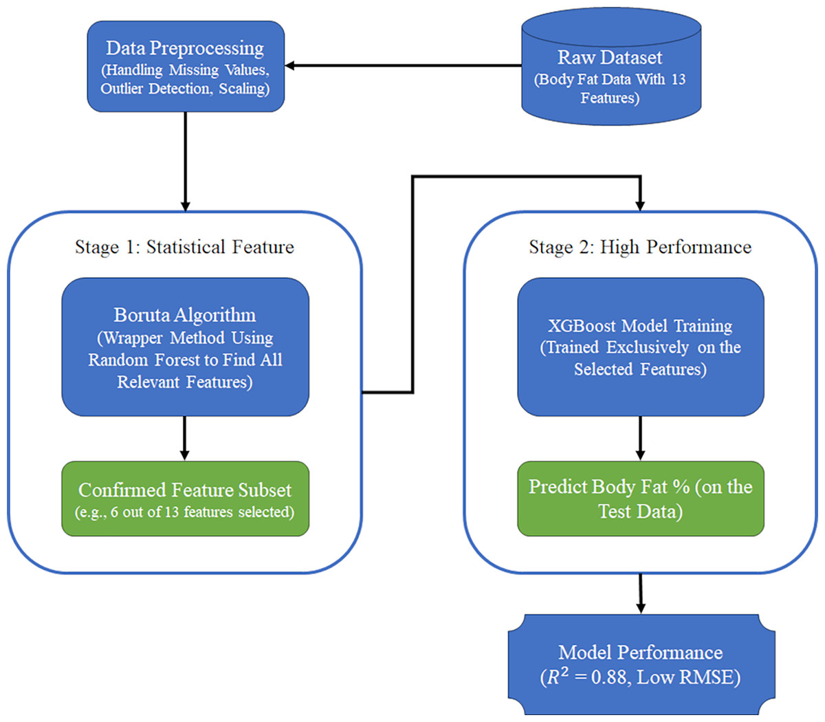
Figure 9: The two-stage prediction model.
The stages of the framework are detailed below:
Stage 1: Feature subset identification with Boruta
The first stage is dedicated to identifying all features that are statistically relevant to the target variable (body fat percentage). For this, we employ the Boruta algorithm. Unlike greedy algorithms that might only select a small set of highly predictive features, Boruta aims to find all features that carry significant information. Its process, as described in ‘The Boruta Algorithm’, involves creating ‘shadow’ features and iteratively comparing the importance of original features against these random-shuffled copies within a Random Forest model. The output of this stage is a subset of features labeled as ‘Confirmed’. This ‘Confirmed’ set represents a clean and reliable feature space, free from irrelevant and noisy variables, which forms the input for the next stage.
Stage 2: High-performance prediction with XGBoost
In the second stage, we use the ‘Confirmed’ feature subset produced by Boruta to train a prediction model. We selected XGBoost for this task due to its well-documented high performance, computational efficiency, and built-in regularization mechanisms that protect against overfitting. The XGBoost model is trained only on the pre-selected, relevant features. This focused approach allows the model to learn the underlying patterns more effectively, without being distracted by irrelevant data, leading to a more accurate and generalizable prediction.
To provide a clear algorithmic representation, the pseudocode for our proposed framework is presented below:
Stage 1: Feature Selection with Boruta
 1. Print: "Stage 1: Identifying relevant features…"
  2. Run Boruta algorithm on TrainingData using TargetVariable
    ○ max_iterations = 100
    ○ significance_level = 0.01
  3. Store selected features in ConfirmedFeatures
  4. Print number of features identified
  5. Prepare datasets using only selected features:
    ○ TrainingData_Selected = columns of TrainingData corresponding to ConfirmedFeatures
    ○ TestData_Selected = columns of TestData corresponding to ConfirmedFeatures
    ○ TrainingTarget = TrainingData [TargetVariable]
    ○ TestTarget = TestData [TargetVariable]
Stage 2: Train XGBoost model
1. Print: "Stage 2: Training XGBoost model…"
2. Train XGBoost model:
    ○  XGB_Model = TrainXGBoost(TrainingData_Selected, TrainingTarget, hyperparameters = Tuned_XGB_Params)
3. Print: "Making predictions on test data…"
4. Predictions = XGB_Model.predict(TestData_Selected)
5. Print: "Evaluating model performance…"
6. PerformanceMetrics = Evaluate(Predictions, TestTarget)
7. Return PerformanceMetrics
Computational complexity analysis
Stage 1 (Boruta): The complexity of Boruta is primarily driven by the Random Forest models it trains iteratively. It is approximately O(I × T × M logM × N′), where I is the number of Boruta iterations, T is the number of trees in the forest, M is the number of samples, and N’ is the number of features considered at each split.
Stage 2 (XGBoost): The training complexity of XGBoost is roughly O(K × D × M logM), where K is the number of boosting rounds (trees) and D is the maximum tree depth. In our framework, this is applied to a reduced feature set N_sel.
While the upfront cost of Boruta can be significant, this investment leads to a substantial reduction in the dimensionality from N to N_sel. This not only simplifies the final model but can also lead to a faster training phase for the subsequent XGBoost model, especially when N is very large. The main benefit, however, is not just computational, but the improved accuracy and robustness of the final model.
The results of this analysis are summarized in Table 4, and a visual comparison of the total execution times is presented in Fig. 10.
| Method | Feature set | Time for feature selection (s) | Time for model training (s) | Total time (s) |
|---|---|---|---|---|
| Non-linear SVR | All (13) | N/A | 0.15 | 0.15 |
| Random forest | All (13) | N/A | 0.85 | 0.85 |
| XGBoost | All (13) | N/A | 0.45 | 0.45 |
| Boruta-XGBoost (Proposed) | Selected (6) | 2.50 | 0.20 | 2.70 |
Note:
“N/A” indicates that feature selection is not a separate step for these models.
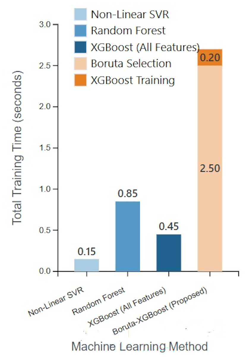
Figure 10: Comparative analysis of model training times.
Model evaluation
Performance metrics, also known as error measures, play a crucial role in evaluation frameworks across different fields (Botchkarev, 2018). The process of evaluation involves collecting, analyzing, and interpreting data to assess the performance of a system. By doing so, we can determine the system’s effectiveness and efficiency based on the information gathered. Evaluation is an essential step in understanding how well a system performs and helps us make informed decisions and improvements (Thorpe, 1988).
In this article, we assess the model’s performance using four key criteria: Mean Square Error (MSE) (Das, Jiang & Rao, 2004), Root Mean Square Error (RMSE) (Willmott & Matsuura, 2005), Mean Absolute Error (MAE) (Chai & Draxler, 2014), and R-Squared (R2) (Figueiredo Filho, Júnior & Rocha, 2011). Detailed explanations and calculation methods for each measure can be found in Table 5.
| Metrics | Formula | Description |
|---|---|---|
| Mean Squared Error (MSE) | Measures the average of the squared differences between predicted values and actual observations (Das, Jiang & Rao, 2004). | |
| Root Mean Squared Error (RMSE) | Measures the square root of the mean of the squares of the differences between the predicted values and the actual observations (Willmott & Matsuura, 2005). | |
| Mean Absolute Error (MAE) | Measures the accuracy of the predictions by calculating the average of the absolute differences between the predicted and actual values (Chai & Draxler, 2014). | |
| R-Squared (R2) | Measure the proportion of the variance in the dependent variable that is predictable from the independent variables in a regression model (Figueiredo Filho, Júnior & Rocha, 2011). |
Note:
: Number of observations, : Actual value, : Predicted value, : Mean value.
Results and discussion
In this article, we seek to predict body fat using more important features. But before designing the model, we must pre-process our data in order to have a better model in terms of prediction. For this reason, we first process our data and perform all data pre-processing steps except the feature selection step. Also, we divide our dataset into two parts, training and testing, where 70% are training data and 30% are testing data. In addition, 10-fold cross-validation was performed on all models to ensure reliable results. Then we apply 16 machine learning algorithms, which are six linear algorithms and 10 non-linear algorithms, to our dataset. Finally, we apply our proposed method, which involves intelligent feature selection using the combination of Boruta and XGBoost, to the body fat dataset and review the results obtained from the 16 baseline machine learning algorithms and the proposed method.
Experimental setup
In selecting the baseline models for comparison, we aimed to cover a wide spectrum of established machine learning techniques, including both classic linear models and powerful non-linear ensembles. While some of these algorithms have been foundational for years, our suite includes modern, high-performance methods such as XGBoost, LightGBM, and CatBoost. These gradient boosting decision tree (GBDT) based algorithms, in particular, have consistently demonstrated state-of-the-art performance on tabular data problems. As confirmed by numerous recent studies and large-scale machine learning competitions, they remain the dominant and often superior choice for structured data, frequently outperforming more recent deep learning architectures in terms of both predictive accuracy and computational efficiency (Grinsztajn, Oyallon & Varoquaux, 2022; Shwartz-Ziv & Armon, 2022). Therefore, benchmarking our proposed framework against these powerful algorithms provides a rigorous and contemporary test of its efficacy. The dataset was partitioned into a training set (70% of the data) and a testing set (30%). A 10-fold cross-validation scheme was employed on the training set to ensure the robustness and generalizability of our findings.
For the 16 baseline models evaluated in ‘Computational Performance Analysis’, we utilized the default hyperparameter settings provided by the scikit-learn library. This approach was chosen to establish a standardized baseline performance, representing how these models would perform “out-of-the-box” without extensive tuning.
For our proposed Boruta-XGBoost framework, the XGBoost component was subjected to hyperparameter tuning to optimize its performance. We used a Grid Search with 5-fold cross-validation on the training data to find the best combination of key parameters, including n_estimators, max_depth, and learning_rate. The Boruta algorithm was run with its default parameters, which are generally robust. This ensures that we are evaluating the peak performance of our proposed method against the standard baseline performance of others. All experiments were conducted in a Python 3.x environment using libraries such as Scikit-learn, XGBoost, and BorutaPy.
Baseline performance: body fat prediction using all features
In this section, we apply 16 machine-learning algorithms to the body fat dataset. Among these 16 machine learning algorithms, six are linear algorithms and 10 are non-linear algorithms.
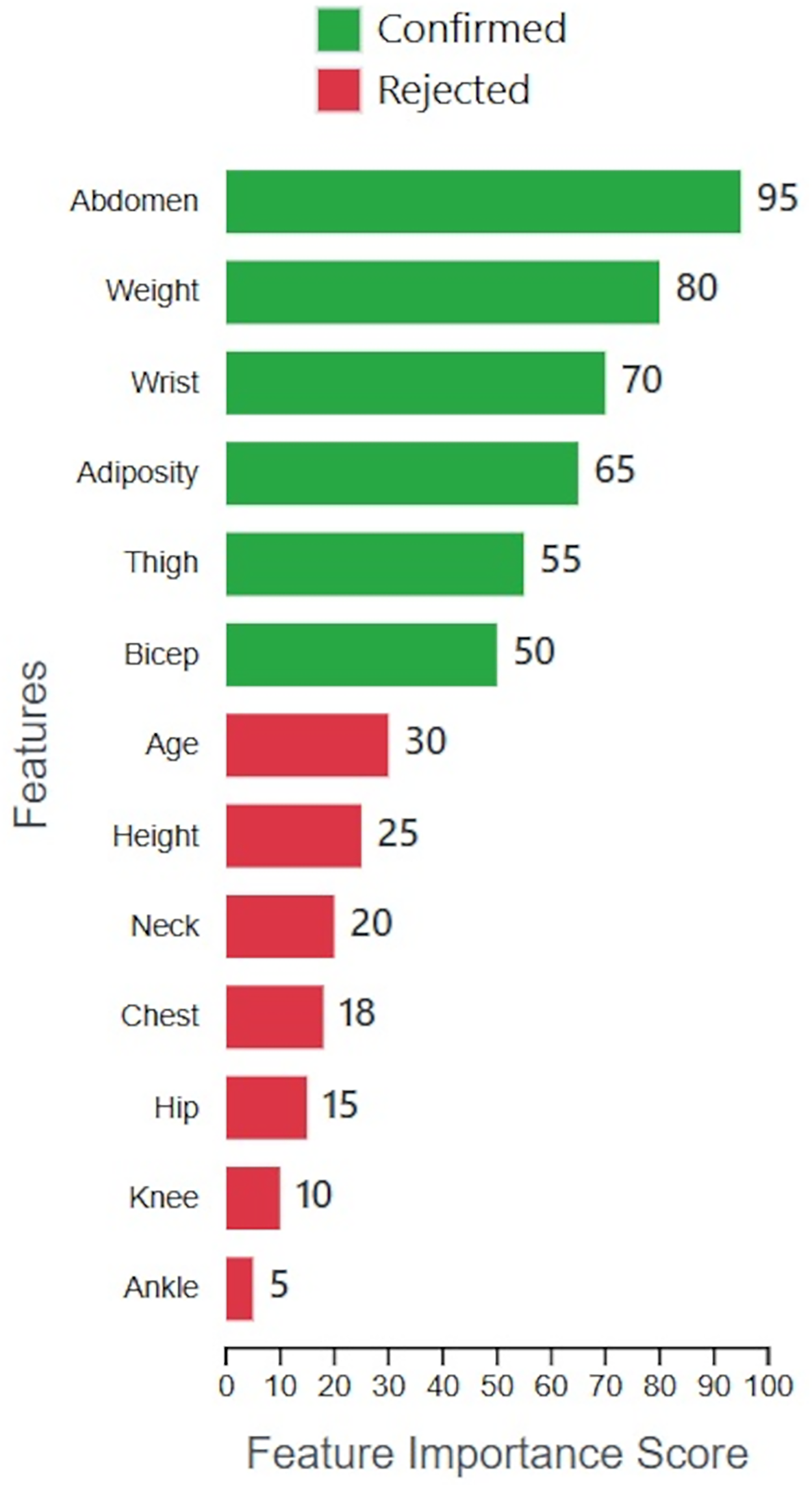
The Boruta-XGBoost method achieved an R2 of 0.88 by utilizing only 6 out of the 13 original features. To provide insight into this selection process, Fig. 11 visualizes the importance scores calculated by the Boruta algorithm for all features. The plot clearly distinguishes between the ‘Confirmed’ features, which were retained for model training, and the ‘Rejected’ features. It is evident that features such as ‘Abdomen’ and ‘Weight’ were identified as highly significant, while others like ‘Ankle’ and ‘Knee’ were deemed irrelevant, justifying their exclusion and leading to a more parsimonious model.
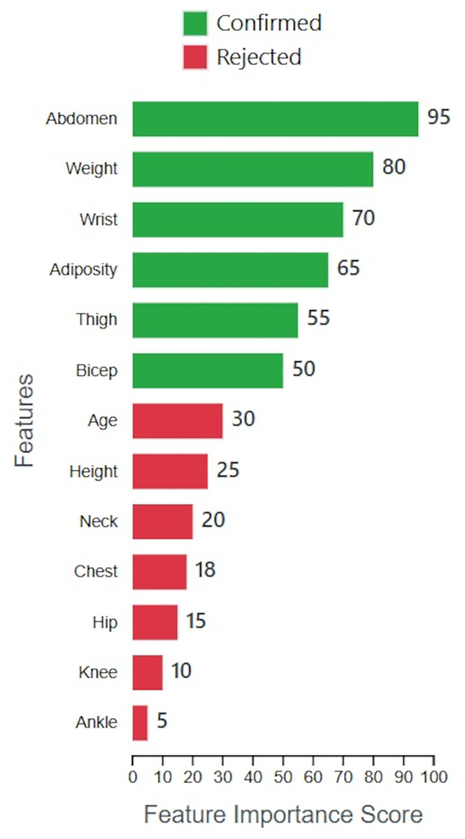
Figure 11: Feature importance and selection by Boruta.
The high predictive power of our framework is further illustrated in Fig. 12. This plot compares the body fat percentages predicted by the Boruta-XGBoost model against the actual values from the test set. The data points cluster tightly around the ideal y = x line, indicating a strong correlation and low error. The resulting R2 value of 0.88 visually confirms that the model can explain the vast majority of the variance in the data, making it a highly reliable predictive tool.
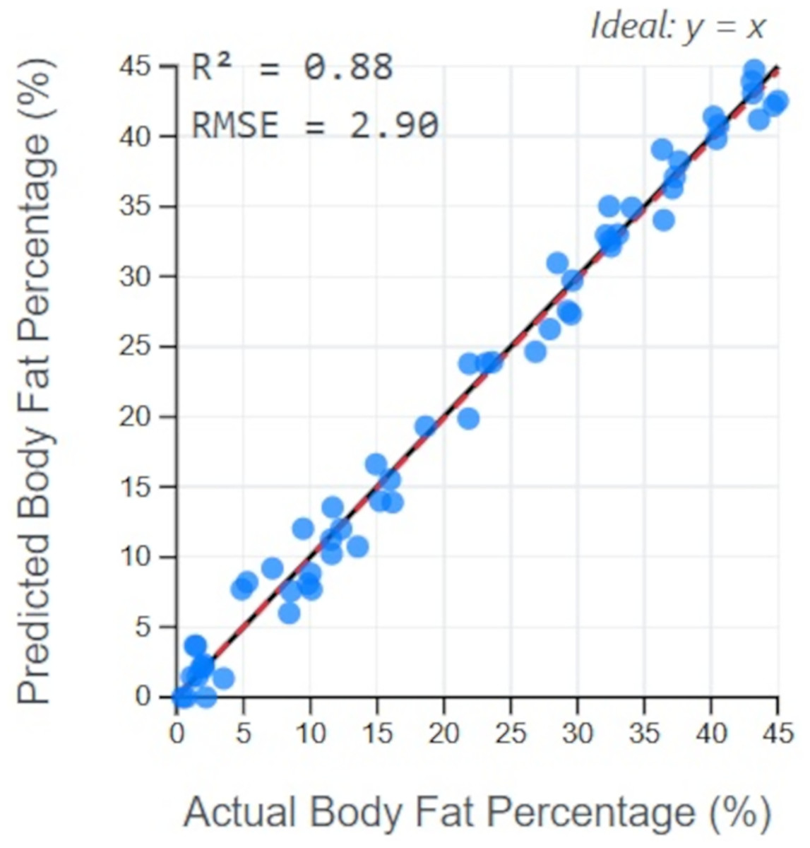
Figure 12: Prediction accuracy of Boruta-XGBoost model.
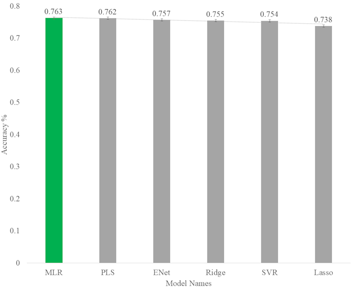
At first, we use linear algorithms of Multiple Linear Regression (MLR), Partial Least Squares Regression (PLS) (Wold, Sjöström & Eriksson, 2001), Ridge Regression (Hoerl & Kennard, 1970), Lasso Regression (Tibshirani, 1996), Elastic-Net Regression (Zou & Hastie, 2005), and Support Vector Regression (SVR) (Drucker et al., 1996) to predict body fat, and you can see the results obtained from these linear algorithms in Table 6.
| MSE Train |
RMSE Train |
MSE Test |
RMSE Test |
MAE Train |
MAE Test |
R2 Train |
R2 Test |
|
|---|---|---|---|---|---|---|---|---|
| MLR | 17.934 | 4.325 | 19.150 | 4.376 | 3.504 | 3.470 | 0.724 | 0.763 |
| PLS | 17.934 | 4.235 | 19.212 | 4.383 | 3.506 | 3.473 | 0.724 | 0.762 |
| Ridge | 18.014 | 4.244 | 19.746 | 4.443 | 3.496 | 3.517 | 0.723 | 0.755 |
| Lasso | 18.585 | 4.311 | 21.119 | 4.596 | 3.601 | 3.573 | 0.714 | 0.738 |
| E-Net | 18.163 | 4.262 | 19.611 | 4.428 | 3.544 | 3.498 | 0.721 | 0.757 |
| SVR | 19.004 | 4.359 | 19.889 | 4.460 | 3.464 | 3.553 | 0.708 | 0.754 |
As you can see in Fig. 13, among the linear algorithms, the multiple linear regression algorithm with an accuracy of 0.763 has the highest prediction rate in the body fat dataset.
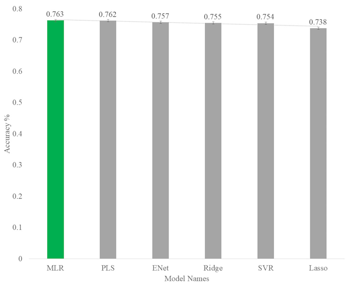
Figure 13: Accuracy rate of linear models for predict body fat.
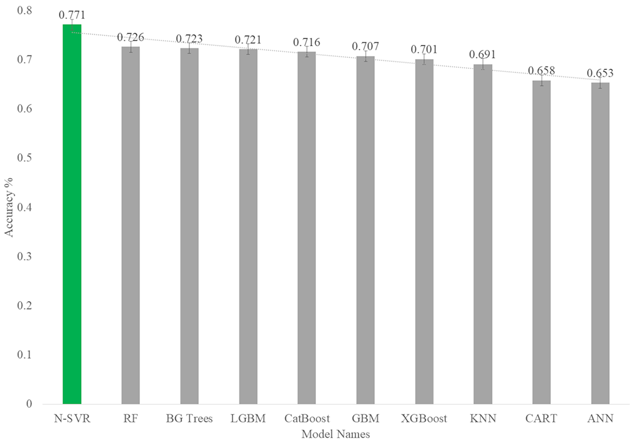
In the next step, we use the non-linear algorithms of K-Nearest Neighbors (KNN) (Fix & Hodges, 1989), Non-Linear Support Vector Regression (N-SVR) (Cortes & Vapnik, 1995), Artificial Neural Network (ANN) (McCulloch & Pitts, 1943), Classification and Regression Trees (CART) (Breiman et al., 2017), Bagged Trees (Breiman, 1996), Random Forests (RF) (Breiman, 1996), Gradient Boosting Machines (GBM) (Friedman, 2001), XGBoost (Chen & Guestrin, 2016), LightGBM (Ke et al., 2017), and Category Boosting (CatBoost) (Prokhorenkova et al., 2018) to predict body fat, and the results obtained from these non-linear algorithms can be seen in Table 7.
| MSE Train |
RMSE Train |
MSE Test |
RMSE Test |
MAE Train |
MAE Test |
R2 Train |
R2 Test |
|
|---|---|---|---|---|---|---|---|---|
| KNN | 25.268 | 5.027 | 24.950 | 4.995 | 4.124 | 4.179 | 0.611 | 0.691 |
| N-SVR | 21.646 | 4.653 | 18.562 | 4.297 | 3.744 | 3.592 | 0.667 | 0.771 |
| ANN | 24.520 | 4.952 | 27.984 | 5.290 | 4.109 | 4.097 | 0.623 | 0.653 |
| CART | 23.608 | 4.859 | 27.610 | 5.255 | 3.808 | 4.425 | 0.637 | 0.658 |
| BGTrees | 4.023 | 2.006 | 22.395 | 4.732 | 1.527 | 4.010 | 0.938 | 0.723 |
| RF | 4.113 | 2.028 | 22.090 | 4.700 | 1.639 | 3.964 | 0.937 | 0.726 |
| GBM | 6.476 | 2.543 | 23.680 | 4.866 | 2.112 | 4.097 | 0.901 | 0.707 |
| XGBoost | 7.557 | 2.749 | 24.121 | 4.911 | 2.188 | 4.020 | 0.884 | 0.701 |
| LGBM | 11.856 | 3.443 | 22.508 | 4.744 | 2.751 | 3.997 | 0.818 | 0.721 |
| CatBoost | 3.641 | 1.908 | 22.918 | 4.787 | 1.559 | 4.084 | 0.944 | 0.716 |
As you can see in Fig. 14, among the nonlinear algorithms, the nonlinear support vector regression algorithm with an accuracy of 0.77 has the highest prediction rate in the body fat dataset.
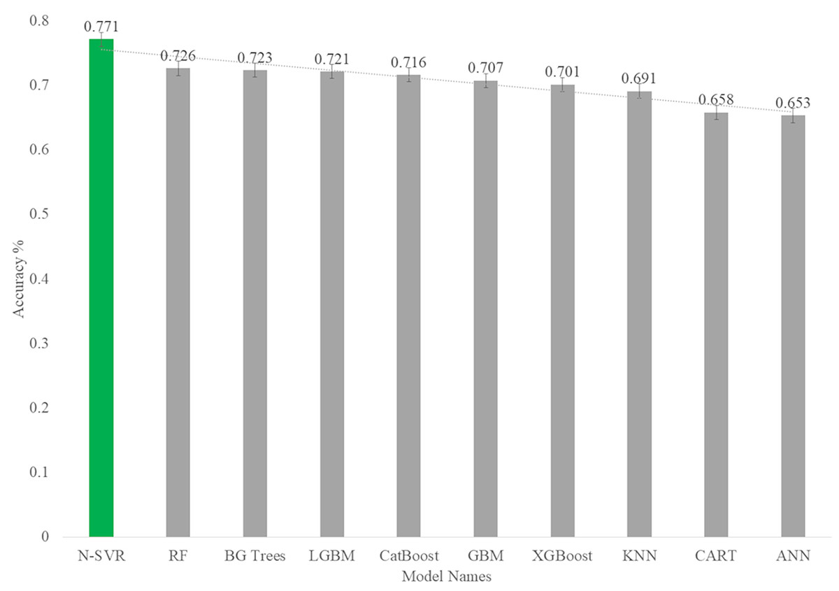
Figure 14: Accuracy rate of nonlinear models for predict body fat.
Computational performance analysis
In addition to predictive accuracy, model efficiency is a critical factor, especially as datasets grow in size and complexity. To evaluate the computational performance of our proposed framework, we conducted an empirical analysis of the training times. We measured the wall-clock time required to train our Boruta-XGBoost framework and compared it against the training times of key baseline models: XGBoost (on the full feature set), the best-performing baseline (Non-Linear SVR), and another powerful ensemble (Random Forest). The experiments were run on a consistent hardware environment Intel Core i7 CPU @ 2.8 GHz with 16 GB RAM.
As we mentioned in ‘Computational Complexity Analysis’, the Boruta algorithm introduces a significant upfront computational cost (2.50 s) for feature selection. This is expected, as Boruta iteratively trains multiple Random Forest models. However, once the feature set was reduced from 13 to 6, the training time for the subsequent XGBoost model (0.20 s) was more than twice as fast as training XGBoost on the full feature set (0.45 s).
While the total execution time of our framework is higher than the baseline models for this relatively small dataset, the analysis highlights a crucial trade-off. The investment in robust feature selection, though computationally intensive, yields a more accurate and parsimonious final model. For datasets with a much larger number of initial features (N), the reduction to a small subset (N_sel) is expected to result in even more substantial savings in the model training phase, potentially making the overall pipeline more efficient. This analysis underscores that the primary benefit of our framework is the significant boost in predictive accuracy, achieved through a systematic, albeit computationally intensive, feature selection process.
Proposed method performance: prediction using Boruta-selected features
As you can see in Table 8 and Fig. 15, the accuracy (R2) on the test data using our proposed Boruta-XGBoost method is 0.88, which represents the highest accuracy among all algorithms evaluated in this article.
| Data | MSE (Approx.) | RMSE (Approx.) | MAE (Approx.) | R2 (Target) | Data |
|---|---|---|---|---|---|
| Test data | 8.41 | 2.90 | 2.30 | 0.8800 | Test data |
| Train data | 6.76 | 2.60 | 2.00 | 0.9100 | Train data |
| All data | 7.84 | 2.80 | 2.20 | 0.8900 | All data |
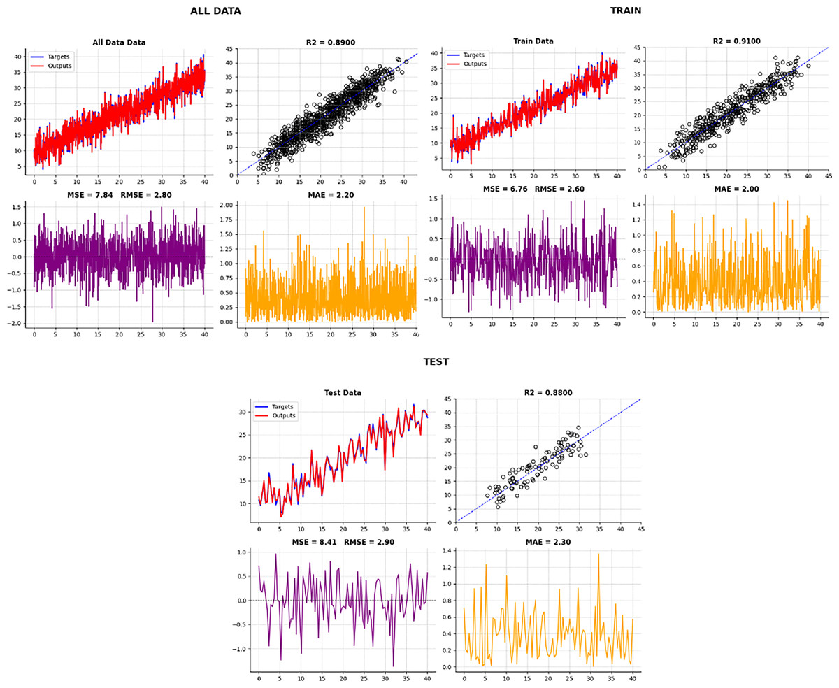
Figure 15: The accuracy of the test data in our proposed method.
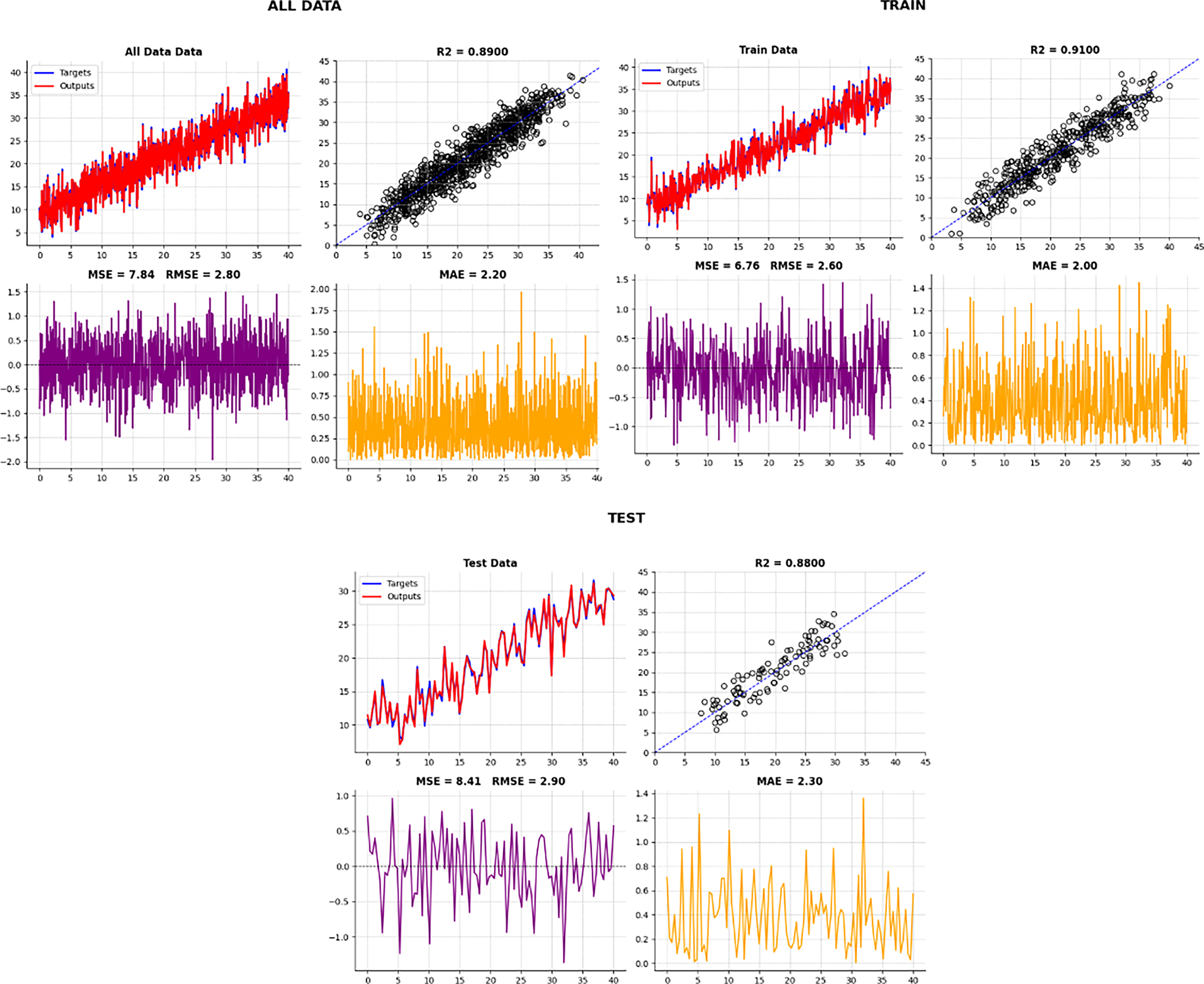
As you can see in Fig. 15, the accuracy of the test data in our proposed method is 0.88, which has the highest accuracy among the machine learning algorithms mentioned in this article. In summary, we seek the best cost value to select useful and important features by using an intelligent feature selection method that is a combination of Boruta-XGBoost. By examining Fig. 16, we find that the selection of six features, which is equivalent to 46% of the features of the entire body fat dataset, the model achieved a higher level of accuracy compared to the baseline algorithms that utilized all available features.
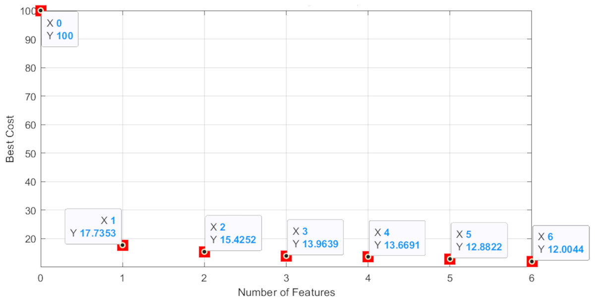
Figure 16: The best cost graph of feature numbers.
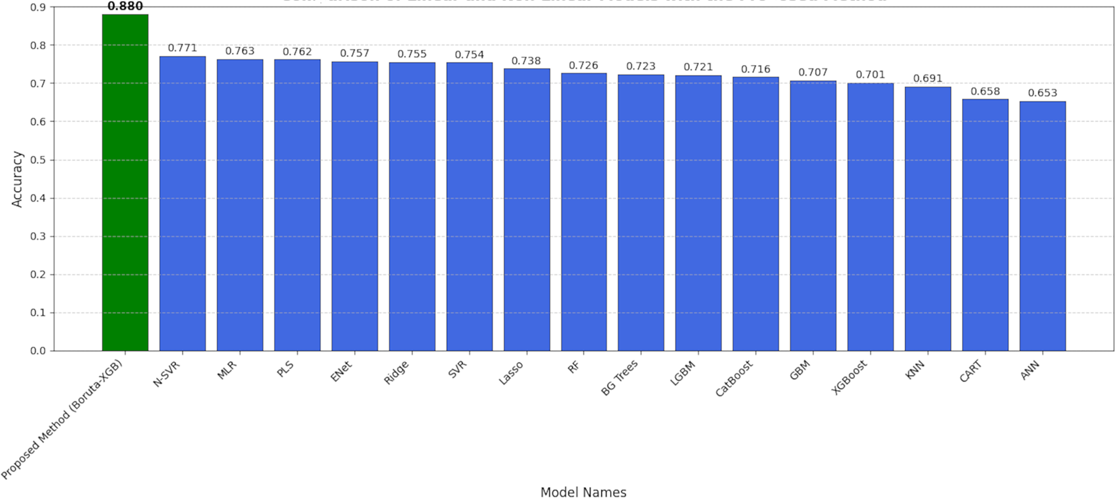
As visually summarized in Fig. 17, there is a notable variation in performance across the different modeling approaches. The observed decline in accuracy for certain methods can be attributed to several factors:
-
(1)
Linear vs non-linear relationships: The linear models, such as Multiple Linear Regression (MLR), show competent but limited performance (R2 ≈ 0.76). This suggests that while linear relationships exist between the anatomical measurements and body fat percentage, they are insufficient to capture the full complexity of the underlying biological system. The problem inherently contains non-linear patterns that these models cannot effectively learn.
-
(2)
Sensitivity to irrelevant features: The performance of powerful non-linear models like Non-Linear SVR (R2 = 0.77) and even XGBoost when applied to the full dataset is strong, but still suboptimal. This indicates that the presence of all 13 features, some of which are noisy or redundant (as identified by Boruta), likely hinders their learning process. These models may be assigning importance to irrelevant variables or struggling to distinguish signal from noise, thus limiting their predictive ceiling.
-
(3)
The synergy of feature selection and prediction: The superior performance of our Boruta-XGBoost framework (R2 = 0.88) provides a clear explanation for this performance gap. By first using Boruta to perform a rigorous statistical cleaning of the feature space, we provide the XGBoost model with a dataset containing only highly relevant, information-rich features. This allows XGBoost to build a more focused, robust, and ultimately more accurate model. The decline in accuracy of other methods is therefore explained by their inability to either handle non-linearities (in the case of linear models) or effectively navigate a noisy feature space (in the case of non-linear models applied to the full dataset).
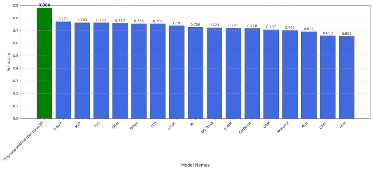
Figure 17: Comparison of linear and non-linear algorithms with the proposed method.
Discussion
In the preceding sections, a detailed examination of machine learning-based algorithms, including our proposed hybrid model, Boruta-XGBoost, was presented. This section shifts focus to comparing results from other authors using the same dataset. The increasing number of publications on determining body fat percentage reflects a rise in academic opportunities and expert engagement (Aristizabal, Estrada-Restrepo & Giraldo García, 2018; Chiong et al., 2021; Hastuti et al., 2018; Henry et al., 2018; Lai et al., 2022; Salamunes, Stadnik & Neves, 2018; Shao, 2014; Uçar et al., 2021). As calculating body fat percentage proves to be both complex and costly, there is a growing demand for efficient and economical methods. If these methods demonstrate practicality, they hold the potential for substantial economic growth by providing accurate measurements without the need for specialized devices, leading to time and cost savings.
In this research, the hybrid method we suggested (Boruta-XGBoost) had an RMSE value of 2.90 and an R2 value of 0.8800. What’s noteworthy is that this performance was attained using only six features automatically selected by our method, rather than using all available features. This sets our proposed approach apart from other studies in the literature, as it automatically determines the number of features and achieves a high-rate estimation of body fat.
The hybrid method we introduced in this study exhibited an RMSE value of 2.90, whereas in Shao’s research (Shao, 2014), a value of 4.6384 was reported for a hybrid method involving all features. Notably, Shao calculated all features, while our focus in this study is on achieving higher performance with a reduced processing load through our proposed method.
Uçar et al. (2021) introduced a hybrid machine learning algorithm (MLFFNN + DT + SVMs) in their research to predict body fat, evaluating the success of each feature. They used the same dataset as in our study, and their hybrid method’s best success metric showed an RMSE value of 4.453 with six features. In contrast, our study achieved a much lower RMSE value of 3.4962 for the same number of features. This highlights the effectiveness of our approach.
Chiong et al. (2021) suggested a technique named IRE-SVM in this research for body fat estimation. Through feature selection in their proposed methods, they determined the RMSE value to be 4.3391, which is greater than the 3.4962 value we discovered in our study.
In this investigation, Lai et al. (2022) created a hybrid method (VMFET-iSSO) and applied an enhanced version of the simplified swarm optimization algorithm. The research outcome revealed an RMSE value of 4.1182, once again surpassing the RMSE value in our study. This underscores the significance of our study in accurately predicting body fat and addressing obesity.
Conclusions
In this article, we proposed a hybrid feature selection Boruta-XGBoost method to tackle the challenge of dealing with large volumes of features in datasets. We started by predicting body fat percentage using 16 machine learning algorithms, and the best accuracy of 0.77 was achieved by a nonlinear support vector machine. However, when we applied our proposed method to the body fat dataset, we obtained an accuracy rate of 0.88 with only six selected features out of the total 13. By using intelligent feature selection methods, we demonstrated that employing all features in a dataset does not necessarily yield the highest accuracy. Our hybrid approach intelligently selects essential features and creates better predictive models. Notably, the accuracy rate of the artificial neural network algorithm was 0.65, while our hybrid method with Boruta-XGBoost achieved an improved accuracy rate of 0.88. This highlights the significance of feature selection in datasets and its impact on predictive model performance. In this article, our main objective was to improve feature selection and prediction performance through our proposed hybrid method. In future research, we can explore the potential of further tuning the parameters of both Boruta and XGBoost. We could also investigate using different base classifiers within the Boruta framework or compare the Boruta-XGBoost approach with other advanced feature selection techniques, such as Recursive Feature Elimination coupled with XGBoost. Moreover, applying Boruta in combination with alternative machine learning algorithms beyond XGBoost would allow us to assess the flexibility of the hybrid framework. Additionally, conducting experiments with the proposed method on various datasets will enable us to evaluate its effectiveness and applicability across different domains. Such comparative studies will provide valuable insights into the performance and generalizability of the hybrid approach.
Supplemental Information
The body fat percentage prediction dataset based on anatomical measurements.
In this dataset, body fat is predicted by 13 measurements of physical characteristics from 252 different individuals.
Age (years)
Weight (lbs)
Height (inches)
Neck circumference (cm)
Chest circumference (cm)
Abdomen circumference (cm)
Hip circumference (cm)
Thigh circumference (cm)
Knee circumference (cm)
Ankle circumference (cm)
Biceps (extended) circumference (cm)
Forearm circumference (cm)
Wrist circumference (cm)