DeepCLSMOTE: deep class-latent synthetic minority oversampling technique

Suvaporn Homjandee; Krung Sinapiromsaran

doi:10.7717/peerj-cs.3461

DeepCLSMOTE: deep class-latent synthetic minority oversampling technique

Suvaporn Homjandee , Krung Sinapiromsaran

Department of Mathematics and Computer Science, Faculty of Science, Chulalongkorn University

DOI: 10.7717/peerj-cs.3461

Published: 2026-02-06
Accepted: 2025-11-18
Received: 2025-06-05

Academic Editor: Consolato Sergi

Subject Areas: Artificial Intelligence, Computer Vision, Data Mining and Machine Learning, Neural Networks
Keywords: Deep learning, Imbalanced datasets, Synthetic minority oversampling technique (SMOTE), Data augmentation, Autoencoder, Latent space, Class separability, Image classification, Representation learning, DeepCLSMOTE

Copyright: © 2026 Homjandee and Sinapiromsaran
Licence: This is an open access article distributed under the terms of the Creative Commons Attribution License, which permits unrestricted use, distribution, reproduction and adaptation in any medium and for any purpose provided that it is properly attributed. For attribution, the original author(s), title, publication source (PeerJ Computer Science) and either DOI or URL of the article must be cited.

Cite this article: Homjandee S, Sinapiromsaran K. 2026. DeepCLSMOTE: deep class-latent synthetic minority oversampling technique. PeerJ Computer Science 12:e3461 https://doi.org/10.7717/peerj-cs.3461

The authors have chosen to make the review history of this article public.

Abstract

Deep learning models often exhibit bias when trained on imbalanced datasets, tending to favor majority classes. While Deep Synthetic Minority Over-sampling Technique (DeepSMOTE) mitigates this challenge by generating synthetic minority class images within an autoencoder’s latent space, the proposed architecture achieves further performance enhancement through the optimization of the latent space structure. This strategy introduces a composite loss function that minimizes intra-class distances while maximizing inter-class distances by incorporating class centroid information into the autoencoder training process. The approach was evaluated on six benchmark image datasets (MNIST, Fashion-MNIST, EMNIST, SVHN, GTSRB, and CIFAR10) with severe class imbalance ratios of 750:1, using five-fold cross-validation. Results demonstrate that Deep Class-Latent Synthetic Minority Oversampling Technique (DeepCLSMOTE) consistently outperforms baseline methods, including Balancing Generative Adversarial Network (BAGAN) and DeepSMOTE across all evaluation metrics, achieving statistically significant improvements in macro-average accuracy, precision, recall, and F1-measure. The enhanced performance is attributed to improved discriminative feature extraction in the optimized latent space, resulting in superior classification performance on highly imbalanced image datasets, particularly for critical minority classes.

Introduction

Deep learning has achieved remarkable success across a variety of domains, including image recognition and natural language processing (Sophia, 2024). However, an effective handling of imbalanced datasets constitutes a significant challenge in the application of deep learning, particularly in real-world contexts where a skewed distribution of samples across different classes is prevalent (Krawczyk, 2016; Johnson & Khoshgoftaar, 2019). The problem of class imbalance has long constituted a prominent challenge in the broader field of machine learning, with extensive systematic reviews documenting the various techniques developed to address this issue (Buda, Maki & Mazurowski, 2018; Fernández et al., 2018). Although these foundational methods are established, researchers have specifically investigated the unique challenges deep learning models encounter with imbalanced data, noting their propensity to exhibit bias towards the majority class and yield suboptimal performance in critical minority classes (Joloudari et al., 2023). This inherent bias can substantially restrict the effectiveness of deep learning models in applications where accurate prediction of the minority class is crucial.

Classical deep learning models, including feedforward neural networks (NN), convolutional neural networks (CNN) and recurrent neural networks (RNN), face several limitations when dealing with imbalanced datasets (Johnson & Khoshgoftaar, 2019; Joloudari et al., 2023). Two primary issues arise in this context (Goodfellow, Bengio & Courville, 2016). First issue is the bias towards the majority class. Due to the abundance of samples from the dominant class, the model prioritizes learning its features, resulting in poor generalization for underrepresented classes. Second issue is high misclassification rate for minority classes. The misclassification of minority class images can entail severe consequences, especially in critical domains such as healthcare. It is imperative to minimize false negatives for minority classes, even at the expense of some accuracy on the majority class (Aubaidan et al., 2025).

Addressing the challenge of imbalanced datasets in deep learning has prompted the development of various techniques, typically categorized as data-level methods and algorithm-level methods. Data-level methods are centered on modifying the training data distribution to mitigate class imbalance. Traditional approaches include resampling techniques applied in the original data space. Oversampling methods, such as Random Oversampling, replicate instances of minority classes, while synthetic oversampling techniques like the original Synthetic Minority Over-sampling Technique (SMOTE) (Chawla et al., 2002), generate synthetic instances in the feature space via interpolating between existing minority instances. However, these methods can sometimes lead to overfitting on the minority class or generate samples that lack the complexity and realism of real-world data, particularly for high-dimensional data like images. Undersampling methods, conversely, reduce the number of majority class samples (Lauron & Pabico, 2016), which may result in the loss of potentially valuable information. Beyond simple resampling, more advanced data augmentation strategies have been explored to increase the diversity of minority class samples (Zhang et al., 2024).

Algorithm-level methods, on the other hand, focus on modifying the learning algorithm or the training process itself. A prominent approach in this category is modifying the loss function to make the model more sensitive to minority class errors. Techniques like weighted cross-entropy assign higher weights to minority classes in the loss calculation (Terven et al., 2023). More sophisticated loss functions, such as Focal (Lin et al., 2017) and methods optimizing CNN parameters using analysis of variance (Zou & Wang, 2024), have been designed to dynamically adjust the gradient contribution of different examples or classes during training, thereby focusing more on hard-to-classify or minority instances (Tang et al., 2024). Other algorithm-level strategies include ensemble methods that combine multiple models trained on different data distributions or with different biases (Khan, Chaudhari & Chandra, 2023) and approaches leveraging transfer learning to adapt knowledge from related, potentially more balanced, tasks (Hassan Pour Zonoozi & Seydi, 2022).

In the context of deep learning for image data, considerable recent effort has been directed towards generating synthetic instances to augment the training set, often leveraging the power of deep generative models. Generative adversarial networks (GANs) and variational autoencoders (VAEs) have shown great promise in modeling complex data distributions and generating realistic-looking images (Goodfellow et al., 2014; Kingma & Welling, 2013). Applications of GANs for imbalanced data include methods like Data Augmentation with Balancing GAN (BAGAN) and Generative Adversarial Minority Oversampling (GAMO). BAGAN aims to generate synthetic minority samples by initializing its generator with the decoder of an autoencoder trained on both minority and majority images (Mariani et al., 2018). GAMO, by contrast, is based on a three-player adversarial game between a convex generator, a discriminator, and a classifier network (Mullick, Datta & Das, 2019). However, training stability of GANs can be a significant challenge, leading to extensive research on improved training techniques (Miyato et al., 2018; Salimans et al., 2016; Gulrajani et al., 2017; Arjovsky, Chintala & Bottou, 2017; Heusel et al., 2017). Beyond GANs and VAEs, other deep generative models for images, such as Pixel Recurrent Neural Networks, have also been developed (van den Oord, Kalchbrenner & Kavukcuoglu, 2016).

More recently, research has explored generating synthetic data or manipulating representations in the latent space learned by deep models. DeepSMOTE (Dablain, Krawczyk & Chawla, 2023) is a prominent example of this approach, extending the original SMOTE idea by operating in the latent space of an autoencoder. While DeepSMOTE effectively generates synthetic minority images, it does not explicitly incorporate mechanisms to optimize the structure of this latent space for enhanced class separability. Consequently, this research aims to develop an approach that specifically optimizes the learned latent representations to enhance class separability and improve performance on imbalanced datasets, which addresses these limitations through three principal contributions: First, the integration of class centroid information into the autoencoder architecture enhances understanding of latent space boundaries and relationships. Second, the integrated loss function minimizes the distance between latent vectors and their associated class centroids, thereby promoting intra-class compactness while simultaneously maximizing the distance between centroids of different classes, encouraging inter-class separation. Third, the proposed model outperforms the GAN-based generative model trained on highly imbalanced image datasets, indicating that the incorporation of class centroid information significantly enhances the model’s ability to learn from imbalanced data and make accurate predictions. Thus, the proposed method advances imbalanced learning by optimizing the latent space with class centroids, enhancing class separability and classification accuracy in multi-class image tasks.

Deepclsmote architecture

Considering the limitations of existing approaches, as discussed in the preceding sections, this part of the article introduces the proposed architecture. Its underlying motivation and detailed design are elaborated in the following subsections.

Motivation

Even after employing the DeepSMOTE technique, an encoded feature space may not fully capture the inherent class distributions. This can result in suboptimal generation of minority class instances and diminished classifier performance. Consequently, this necessitates further refinement of the latent space during image generation model training. To address this, we introduce a novel deep learning architecture, a Deep Class-Latent Synthetic Minority Oversampling Technique (DeepCLSMOTE), which, crucially, incorporates class centroid information into the latent space to generate latent representations of the same class in close proximity while separating latent representations of distinct classes, thereby facilitating improved class distribution learning. This approach indirectly addresses challenges similar to those encountered in long-tailed recognition through improved representation learning in the latent space (Xu & Lyu, 2024).

Architecture and design

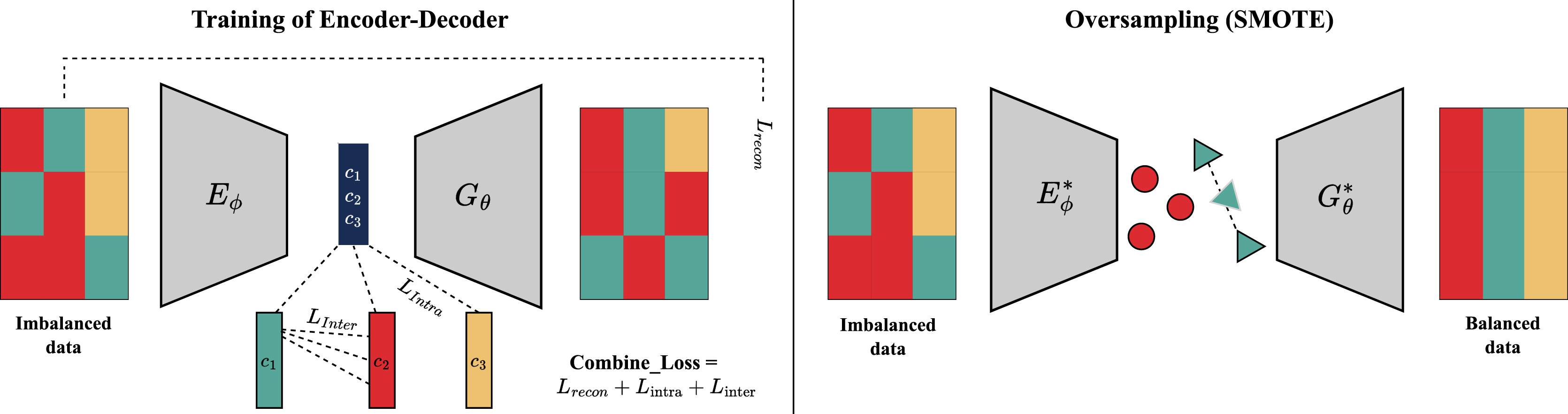
The proposed model architecture depicted in Fig. 1 is trained on an imbalanced dataset. Subsequently, synthetic minority class samples are generated by applying principles similar to SMOTE within the learned latent space using the trained encoder and decoder. Table 1 provides a thorough description and parameter summary of the suggested deep learning architecture. This architecture draws inspiration from DeepSMOTE.

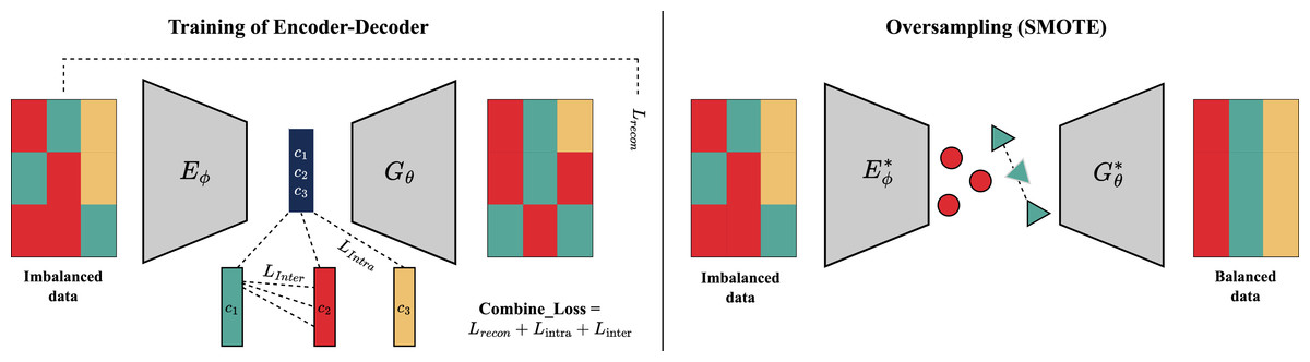
Figure 1: Diagram illustrating an operational flow of the DeepCLSMOTE approach.

Download full-size image

DOI: 10.7717/peerj-cs.3461/fig-1

Table 1:

The autoencoder architecture comprises an encoder and a decoder, where tensor shapes are denoted with “−1” to indicate the flexible batch size.

Encoder summary:			Decoder summary:
Layer (type)	Output shape	Param #	Layer (type)	Output shape	Param #
Conv2d-1	[−1, 64, 14, 14]	1,024	Linear-1	[−1, 25,088]	526,848
LeakyReLU-2	[−1, 64, 14, 14]	0	ReLU-2	[−1, 25,088]	0
Conv2d-3	[−1, 128, 7, 7]	131,072	ConvTranspose2d-3	[−1, 256, 10, 10]	2,097,408
BatchNorm2d-4	[−1, 128, 7, 7]	256	BatchNorm2d-4	[−1, 256, 10, 10]	512
LeakyReLU-5	[-1, 128, 7, 7]	0	ReLU-5	[−1, 256, 10, 10]	0
Conv2d-6	[−1, 256, 3, 3]	524,288	ConvTranspose2d-6	[−1, 128, 13, 13]	524,416
BatchNorm2d-7	[−1, 256, 3, 3]	512	BatchNorm2d-7	[−1, 128, 13, 13]	256
LeakyReLU-8	[−1, 256, 3, 3]	0	ReLU-8	[−1, 128, 13, 13]	0
Conv2d-9	[−1, 512, 1, 1]	2,097,152	ConvTranspose2d-9	[−1, 1, 28, 28]	2,049
BatchNorm2d-10	[−1, 512, 1, 1]	1,024	Tanh-10	[−1, 1, 28, 28]	0
LeakyReLU-11	[−1, 512, 1, 1]	0
Linear-12	[−1, 20]	10,260
Total params: 2,765,588			Total params: 3,151,489

DOI: 10.7717/peerj-cs.3461/table-1

The design choices of DeepCLSMOTE are motivated by the need to effectively address class imbalance in image classification. The model builds build upon the concept of generating synthetic minority class images within the latent space of an autoencoder, a technique previously explored in DeepSMOTE. The autoencoder’s ability to learn a compressed and meaningful representation of the input data enables the generation of new data points that lie within the data manifold. To enhance the effectiveness of latent space manipulation for imbalanced learning, this research introduce optimization of the latent space structure by explicitly considering class centroid information. This approach is motivated by the hypothesis that guiding synthetic sample generation towards regions defined by class centroids can improve the representativeness and diversity of the generated samples, leading to better class separability in the learned feature space. Furthermore, explicit minimization of intra-class distances and maximization of inter-class distances in the latent space is designed to yield more discriminative features, directly addressing the bias towards majority classes prevalent in models trained on imbalanced data. The choice of GAN-based approaches as baselines was driven by their established capability in generating realistic synthetic data, making them a relevant comparison point for evaluating the quality and impact of our latent space optimization strategy.

Therefore, the encoder component processes $28 \times 28$ grayscale images (x) through a series of convolutional layers, each utilizing a $4 \times 4$ kernel, a stride of 2 and a 1-pixel padding. The first layer produces a $14 \times 14$ feature map with 64 channels. The number of channels doubles in each subsequent convolutional layer, leading to a final feature map of size $1 \times 1 \times 512$ . This feature map is flattened and fed into a fully connected layer to generate a 20-dimensional latent vector, y for gray color, and 300-dimension for RGB color image. The decoder component mirrors this process, starting with a fully connected layer that maps the 300-dimensional latent space back to a 512-dimensional feature vector. This vector is then reshaped and fed into a series of deconvolutional layers to progressively upsample the feature maps, culminating in a reconstructed $28 \times 28$ grayscale image. Throughout the network, techniques such as Batch Normalization are applied after convolutional layers to accelerate training and improve stability by reducing internal covariate shift (Ioffe & Szegedy, 2015). For activation functions, we utilize LeakyReLU, which has shown effectiveness in convolutional networks (Xu et al., 2015). Backpropagation algorithm employs a combined loss function consisting of three components. First, a main latent loss measures an error between the input image pixel $x_{i}$ and the reconstructed output image $\hat{x_{i}}$ location within a training batch of size B. It is calculated as Mean Squared Error (MSE, 2008) shows in an equation below:

$L_{r e c o n} = \frac{1}{B} \sum_{i = 1}^{B} ‖ x_{i} - \hat{x_{i}} ‖_{2}^{2} .$

The second loss function involves creating a representative vector for each class to minimize a class-specific latent loss, as defined in $L_{i n t r a}$ . This loss measures the distance between the latent representation ( $c^{j}$ ), and a class-specific latent representation ( ${\tilde{c}}^{j}$ ) generated by a separation from the fully connected layer. This process is applied for all samples within a given class $j$ to minimize the intra-class variance.

$L_{i n t r a} = \sum_{j = 1}^{C} \frac{1}{M_{j}} \sum_{i = 1}^{M_{j}} ‖ {c_{i}}^{j} - {\tilde{c_{i}}}^{j} ‖_{2}^{2}$ where, $N_{j}$ denotes the number of images in class $j$ . For an Equation of $L_{i n t e r}$ , the loss associated with class separation aims to encourage distinct latent representations for different classes. This loss is computed as the inverse of the sum of pairwise Euclidean distances between the class-specific latent representation for classes $j$ and $k$ , denoted as ${\tilde{c}}^{j}$ and ${\tilde{c}}^{k}$ respectively.

$L_{i n t e r} = {[\sum_{k = 1}^{C} \sum_{j = 1}^{C} ‖ {\tilde{c}}^{j} - {\tilde{c}}^{k} ‖_{2}^{2} + ε]}^{- 1} s . t . k \neq j$ where $ε$ represents a small constant (e.g., $1 e - 8$ ) included for numerical stability. This term prevents the loss function from becoming unstable or undefined in cases where the distance between centroids is extremely small.

A simple CNN is employed as a baseline classifier to assess the performance of deep learning techniques on highly imbalanced datasets. The CNN architecture comprises two convolutional layers, each followed by a max pooling layer. These layers are succeeded by fully connected layers, culminating in a classification layer that categorizes the input image. For instance, some effective CNN architectures utilize residual connections to improve training of deep networks (He et al., 2016). The image augmentation based DeepCLSMOTE and CNN classification are available on GitHub (https://github.com/FaiHomjandee/DeepCLSMOTE) and have been archived on Zenodo (Homjandee & Sinapiromsaran, 2025). Further details of the proposed method’s complete procedure can be found in the pseudocode provided in Algorithm 1. For the combined loss function, the weights $λ_{1}, λ_{2}$ and $λ_{3}$ were all empirically set to 1 throughout the experiments, ensuring: maintaining the autoencoder’s primary objective of accurate image reconstruction ( $λ_{1}$ ), providing sufficient gradient signal for centroid-based clustering within classes ( $λ_{2}$ ), and contributing adequate separation force between class centroids without overwhelming other objectives ( $λ_{3}$ ).

Algorithm 1 :

DeepCLSMOTE.

1: Input:

D = {(x_{i}, y_{i})

where

i \in N

2: Parameters: Latent dimension d, learning rate η, batch size B, number of epochs E.

3: Output: A balanced dataset D_bal

4: Phase I: Training the Class-Optimized Autoencoder

5: Initialize Encoder

E_{ϕ}

and Decoder

G_{θ}

with random weights φ and θ.

6: for epoch = 1 to E do

7: for each batch

{(x, y)}

in D do

8: z,

\tilde{c} \leftarrow E_{ϕ} (x)

▹ Encode batch to latent vectors

\hat{x} \leftarrow G_{θ} (z)

▹Reconstruct batch from latent vectors

10:

L_{1} \leftarrow ‖ x - \hat{x} ‖_{2}^{2}

▹ L1 Reconstruction Loss

11:

L_{2} \leftarrow \sum_{j} ‖ c^{j} - {\tilde{c}}^{j} ‖_{2}^{2}

▹ L2 Intra-Class Loss (compactness)

12:

L_{3} \leftarrow \sum_{j \neq k} \frac{1}{‖ {\tilde{c}}^{j} - {\tilde{c}}^{k} ‖_{2}^{2} + ε}

▹ L3 Inter-Class Loss (separation)

13:

L_{t o t a l} \leftarrow λ_{1} L_{1} + λ_{2} L_{2} + λ_{3} L_{3}

▹ Combine losses with weights

λ_{1}, λ_{2}, λ_{3}

14: Update weights

ϕ, θ

using gradient descent:

ϕ, θ \leftarrow ϕ, θ - η \nabla L_{t o t a l}

15: end for

16: end for

17: Phase II: Generating Synthetic Minority Samples

18: for each class = 1 in C do

19: Let

D_{m i n}

be the set of all samples from minority class.

20:

Z_{m i n} \leftarrow E_{ϕ} (D_{m i n})

▹ Encode all minority samples into latent space

21:

S_{l a t e n t} \leftarrow S M O T E (Z_{m i n})

▹ Apply SMOTE algorithm on the latent vectors

22:

S_{i m g} \leftarrow G_{θ} (S_{l a t e n t})

▹ Decode synthetic latent vectors into new images

23:

D_{b a l} \leftarrow D \cup S_{i m g}

▹ Combine original data with synthetic images

24: end for

DOI: 10.7717/peerj-cs.3461/table-6

Regarding the computational complexity of DeepCLSMOTE, it exhibits analogous characteristics to DeepSMOTE due to their shared hybrid architecture, wherein the computational burden is predominantly attributed to the training of deep learning components. The overall complexity can be decomposed into two principal phases. First, the autoencoder training phase represents the most computationally demanding component. The complexity is approximated as $O (E \times N \times C)$ , where E denotes the number of training epochs, N represents the training sample size, and C characterizes the computational complexity of executing a single forward and backward propagation through the autoencoder architecture. Notably, the computation of class centroids within the latent space contributes negligible overhead, as this operation involves straightforward averaging performed once per epoch. Second, the synthetic sample generation phase encompasses forward propagation through the trained decoder network. This process exhibits a complexity of $O (S \times L)$ , where S corresponds to the desired number of synthetic samples, and L represents the computational complexity of the decoder architecture. In the final analysis, the architectural parallels between DeepCLSMOTE and DeepSMOTE result in comparable computational complexities. For both methodologies, deep neural network training serves as the primary computational bottleneck, while the additional centroid computation in DeepCLSMOTE introduces minimal computational overhead.

Materials and Methods

This section outlines the experimental framework used to evaluate the performance of the proposed DeepCLSMOTE method in comparison with baseline generative approaches. Experiments were conducted on a system with an Intel Core i5-10505 CPU, 16 GB RAM, and an Intel UHD Graphics 630 (integrated), using Jupyter version 7.2.2 with Python 3.12.7. Specific details regarding the experimental setup, encompassing the datasets, evaluation metrics, and experimental protocol, are provided in the following subsections.

The selection of techniques implemented in this investigation was guided by both empirical performance considerations and their theoretical relevance to the class imbalance problem. Specifically, the proposed DeepCLSMOTE method was developed as an evolution of DeepSMOTE, which demonstrated the advantage of generating synthetic samples in the latent space of an autoencoder. However, DeepSMOTE lacked explicit latent space structure optimization. To address this, DeepCLSMOTE incorporates class centroid information to guide latent space interpolation, thereby enhancing class separability. This direction was motivated by preliminary benchmarking and recognition of the limitations of purely GAN-based methods (such as BAGAN) in preserving semantic integrity within high-dimensional image spaces. Additionally, DeepCLSMOTE was compared with a plain CNN trained without augmentation to serve as a baseline classifier. The inclusion of these techniques reflects a deliberate strategy to evaluate oversampling effectiveness through latent space manipulation, balancing generative fidelity and class-level discriminability.

Datasets

To ensure a direct and fair comparison with the original Deep SMOTE method, the approach was evaluated on the same set of benchmark datasets, namely MNIST, Fashion-MNIST, SVHN, and CIFAR10. Furthermore, to truly test DeepCLSMOTE’s robustness and scalability on a more complex problem, the EMNIST dataset was included in the evaluation. Unlike the original MNIST, EMNIST has more classes and more intricate character distinctions.

The original DeepSMOTE study also used the high-resolution CelebA dataset as a benchmark. However, due to computational constraints like limited GPU memory and processing power, it was necessary to use a different dataset. The German Traffic Sign Recognition Benchmark (GTSRB) was chosen as a suitable alternative. While less complex than CelebA, GTSRB still represents a realistic and challenging multi-class classification problem, allowing for a good assessment of the model’s performance given the resource limitations. Therefore, six benchmark datasets from the PyTorch libraries (Paszke et al., 2019) were employed in this investigation. Detailed specifications of each dataset are presented below:

MNIST (LeCun, Cortes & Burges, 1998): The MNIST database of handwritten digits is available at http://yann.lecun.com/exdb/mnist/.
Fashion-MNIST (FMNIST) (Xiao, Rasul & Vollgraf, 2017): A dataset of Zalando’s article images can be found at https://github.com/zalandoresearch/fashion-mnist.
EMNIST (Cohen et al., 2017): The Extended MNIST dataset is available at https://paperswithcode.com/paper/emnist-an-extension-of-mnist-to-handwritten.
SVHN (Netzer et al., 2011): The Street View House Numbers dataset is located at http://ufldl.stanford.edu/housenumbers/.
GTSRB (Stallkamp et al., 2012): The German Traffic Sign Recognition Benchmark can be accessed at https://benchmark.ini.rub.de/.
CIFAR10 (Krizhevsky, 2009): The CIFAR-10 dataset is available at https://www.cs.toronto.edu/∼kriz/cifar.html.

The experimental design for this research follows the standard protocol in the established field of long-tailed recognition (Tan et al., 2020). This widely-used approach is critical for simulating real-world scenarios with a substantial class imbalance. To achieve this, the training set is intentionally skewed (datails are in Table 2), while the test set remains balanced. This is a crucial methodological choice, as it provides a fair and unbiased evaluation of the model’s ability to recognize rare minority classes, preventing performance from being artificially inflated by dominant ones. For the training datasets, a modified long-tail distribution was implemented, creating a pronounced imbalance with a ratio of 750:1 between the most and least represented classes. This severe imbalance mimics the challenging conditions often encountered in real-world applications, such as rare diseases in medical diagnosis where cases may comprise less than 1%, or financial datasets where imbalance ratios can exceed 100:1 (Johnson & Khoshgoftaar, 2019; Krawczyk, 2016). A proportional adjustment was made for the GTSRB dataset to accommodate its unique structural characteristics. Furthermore, to test the robustness of the method, no data preprocessing was applied; the models were trained directly on the original pixel values.

Table 2:

Class distribution of imbalanced training datasets.

Dataset/Class	0	1	2	3	4	5	6	7	8	9
M/FM/EM/S/C10	3,000	2,000	1,000	750	500	12	10	8	6	4
GTSRB	1,000	800	600	400	200	12	10	8	6	4

DOI: 10.7717/peerj-cs.3461/table-2

Note:

M/FM/EM/S/C10 represent MNIST, Fashion-MNIST, EMNIST, SVHN, and CIFAR-10 datasets respectively.

The balancing of test was achieved by determining the size of each test class based on the smallest class within the original dataset and the number of cross-validation folds. The number of samples per class within a test fold was calculated as the size of the smallest original class divided by the number of folds ( $N_{s} / k$ ). This approach ensures that no class in the test set is disproportionately large, preventing evaluation bias towards majority classes while guaranteeing representation for all classes, including those rare in the original long-tailed distribution. For example, using 5-fold cross-validation ( $k = 5$ ) with a dataset where the smallest class ( $N_{s}$ ) contained 6,000 samples would result in balanced test sets containing $6, 000 / 5 = 1, 200$ samples per class.

To ensure reliable and generalizable performance evaluation, a five-fold cross-validation protocol was employed. Within each of the five folds, the dataset was partitioned for training and testing, and the model was subsequently trained. Training for each fold was typically conducted for 200 epochs across all datasets. An exception was CIFAR10, which necessitated an extended duration of 300 epochs per fold owing to its comparatively higher image complexity and dataset characteristics.

Evaluation metrics

To facilitate understanding of a confusion matrix in the context of multi-class classification, Table 3 provides an illustrative example, wherein the key terms employed in evaluating classification performance are defined below.

True Positive (TP): The model correctly predicts a positive class.
True Negative (TN): The model correctly predicts a negative class.
False Positive (FP): The model incorrectly predicts a negative class as positive.
False Negative (FN): The model incorrectly predicts a positive class as negative.

Table 3:

Multi-class confusion matrix (Class 1 Perspective).

		Predicted class
		Class 1	Class 2	…	Class $n$
Actual class	Class 1	TP	FN	FN	FN
	Class 2	FP	TN	TN	TN
	…	FP	TN	TN	TN
	Class $n$	FP	TN	TN	TN

DOI: 10.7717/peerj-cs.3461/table-3

However, it is crucial to reiterate this process for all classes and calculate the average TP, FP, TN, and FN values across all classes. Subsequently, we can compute the overall accuracy, precision, recall, and F1-measure for the multi-class classification tasks, as defined in Table 4, where $n$ denote the number of classes.

Table 4:

Classification measures for multi-class evaluation (Grandini, Bagli & Visani, 2020).

Measurers	Formulae	Description
Accuracy	$\frac{\sum_{i = 1}^{n} \frac{T P_{i} + T N_{i}}{T N_{i} + T P_{i} + F N_{i} + F P_{i}}}{n}$	The average class-wise performance of a classifier.
Precision	$\sum_{i = 1}^{n} \frac{\frac{T P_{i}}{T P_{i} + F P_{i}}}{n}$	An average per-class agreement between the true class labels and the predicted class labels assigned by a classifier.
Recall	$\sum_{i = 1}^{n} \frac{\frac{T P_{i}}{T P_{i} + F N_{i}}}{n}$	An average per-class accuracy of a classifier in identifying class labels.
F1-measure	$\frac{2 \cdot (R e c a l l \cdot P r e c i s i o n)}{R e c a l l + P r e c i s i o n}$	Average per-class agreement between the true and predicted class labels.

DOI: 10.7717/peerj-cs.3461/table-4

Experimental protocol

Following the method selection outlined above, a comparative study was conducted to rigorously evaluate the proposed DeepCLSMOTE technique for addressing imbalanced image datasets. In this evaluation, DeepCLSMOTE was compared with two established generative models for minority class augmentation: DeepSMOTE and BAGAN, as well as a Plain CNN model. DeepSMOTE was selected because the proposed method is a direct extension of its architecture. Additionally, BAGAN was chosen to represent GAN-based methods; while other state-of-the-art models like GAMO exist, BAGAN’s use of an autoencoder for initialization makes it a more architecturally similar and relevant benchmark. The Plain CNN serves as a crucial baseline to demonstrate the limitations of standard classification models on imbalanced data. Although computational constraints limited direct implementation to these baselines, our results can be contextualized within the broader imbalanced learning landscape. The original DeepSMOTE study was comprehensively evaluated against numerous state-of-the-art approaches (Dablain, Krawczyk & Chawla, 2023), including algorithm-level methods (Focal Loss, cost-sensitive learning), data-level methods (original SMOTE variants), and ensemble approaches. Our consistent outperformance of DeepSMOTE with statistical significance suggests that DeepCLSMOTE represents a meaningful advancement in latent space optimization for imbalanced learning, positioning our contribution as a competitive approach within the current methodological landscape, though direct comparison with the broader range of techniques would strengthen future validation.

The evaluation process followed a five-fold cross-validation protocol, the overall experimental framework of which is illustrated in Fig. 2. Within each of the five folds, the original imbalanced training data was augmented by applying each generative method to produce synthetic samples for the minority classes, thereby balancing the class distribution for that fold’s training set. Subsequently, a standard deep learning classifier was then trained independently on the balanced training data of each fold and evaluated on the corresponding test fold.

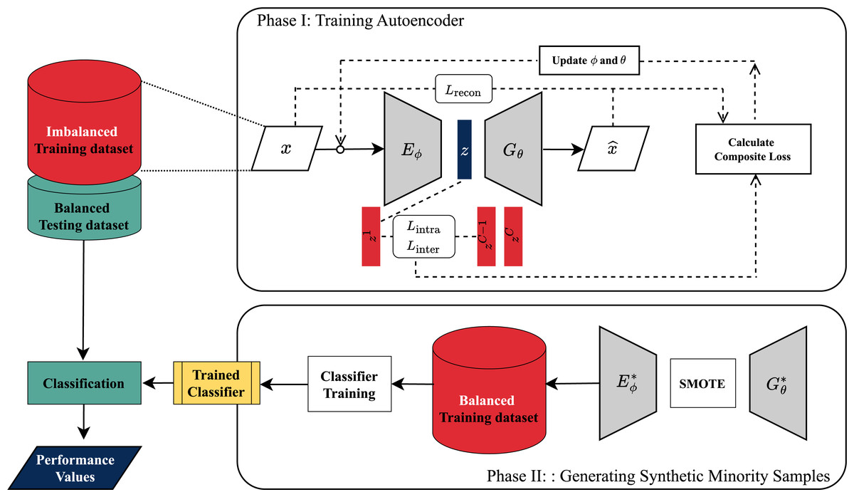
Figure 2: Process flowchart for the DeepCLSMOTE algorithm.
Phase I shows the autoencoder training loop where weights are updated based on the composite loss. Phase II details how the trained model is used with SMOTE to generate new samples and balance the dataset.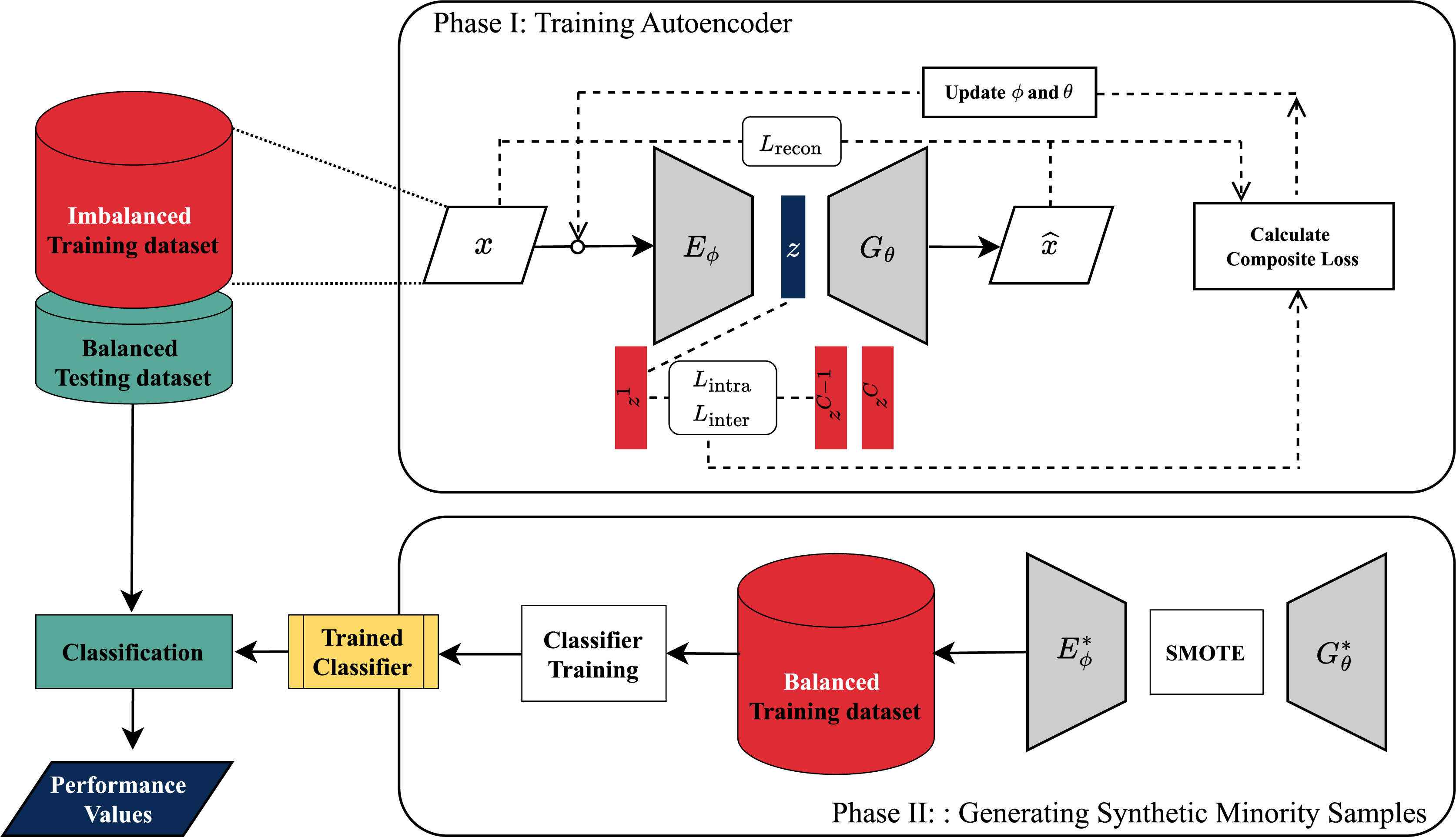

Download full-size image

DOI: 10.7717/peerj-cs.3461/fig-2

The quantitative performance of DeepCLSMOTE and the reference methods was assessed using standard metrics: accuracy, precision, recall, and F1-measure, calculated on the test sets of each fold. To provide a comparative analysis of the overall performance, the following procedure was used: For each evaluation metric and within each of the five folds, the performance of DeepCLSMOTE and the reference methods was ranked. The average rank for each method across the five folds was then computed. These averaged ranks are presented visually in Statistical Ranking and Comparison section. Finally, to determine the statistical significance of the observed performance differences between DeepCLSMOTE and the reference methods, the Wilcoxon Signed-Rank test was employed. This non-parametric statistical test was applied to the per-fold performance scores for each metric.

Results

Emerging from the experimental evaluation, conducted as detailed in this section, are the key findings regarding the performance of the proposed DeepCLSMOTE method and baseline approaches. This section presents a comprehensive analysis and discussion of these results, encompassing both qualitative assessments of synthetic image quality and quantitative performance metrics.

Qualitative assessment of synthetic images

For a qualitative evaluation, this subsection provides generated synthetic image examples for visual evaluation, presented separately for grayscale and RGB datasets in the following sub-subsections. For detailed visual inspection, high-resolution versions of all generated images are available in the complete dataset archived on Zenodo (Homjandee & Sinapiromsaran, 2025).

Grayscale image quality

The visual quality of the generated minority class instances was qualitatively assessed across three methods: BAGAN, DeepSMOTE, and DeepCLSMOTE. Figure 3 presents nine instances of generated imagery for each of the five least frequent minority classes in the original dataset, shown for visual comparison across each dataset.

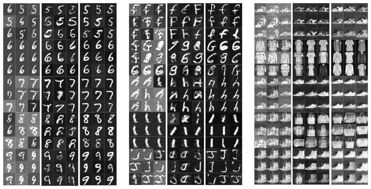
Figure 3: Examples of generated grayscale images of the five rarest minority classes from (A) MNIST, (B) EMNIST, and (C) Fashion-MNIST using BAGAN, DeepSMOTE, and DeepCLSMOTE, respectively (each column showing results from BAGAN, DeepSMOTE, and DeepCLSMOTE).

Download full-size image

DOI: 10.7717/peerj-cs.3461/fig-3

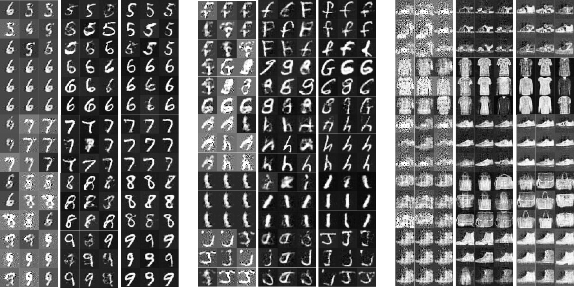
For the MNIST dataset, although digit shapes were produced by BAGAN and DeepSMOTE, the generated outputs often appeared blurry and structurally inconsistent, particularly for complex digits (e.g., ‘5’, ‘8’, and ‘9’). In contrast, significantly sharper and more coherent digits were synthesized by DeepCLSMOTE, exhibiting clearer strokes and minimal noise. A similar observation was noted for the EMNIST dataset. Character samples produced by BAGAN were frequently distorted and challenging to interpret, and DeepSMOTE often resulted in confusion between visually similar letters. DeepCLSMOTE, however, synthesized characters exhibiting improved structure and clarity, particularly for challenging classes such as ‘g’, ‘h’, and ‘j’.

Within the Fashion-MNIST dataset, the generation of fashion items by BAGAN lacked clear form and texture, while DeepSMOTE provided moderate improvements in pattern recognition. The best visual fidelity was achieved by DeepCLSMOTE, which generated clothing items and accessories with clearer outlines and finer details, especially in categories such as shoes, shirts, and handbags.

Generally, it was observed that DeepCLSMOTE consistently produced higher-quality synthetic images in all grayscale datasets evaluated. These synthesized instances demonstrated enhanced intraclass consistency and interclass distinctiveness compared to the other methods, highlighting DeepCLSMOTE’s suitability for augmenting minority classes in imbalanced image classification tasks.

RGB image quality

The performance of DeepCLSMOTE in generating realistic instances for minority classes in RGB image datasets was investigated using three representative datasets: SVHN, GTSRB, and CIFAR10. For each dataset, minority class instances were synthesized using BAGAN, DeepSMOTE, and the proposed DeepCLSMOTE method. As illustrated in Fig. 4, it shows examples of generated images for the five least represented classes in each dataset, based on class distribution in the original training set.

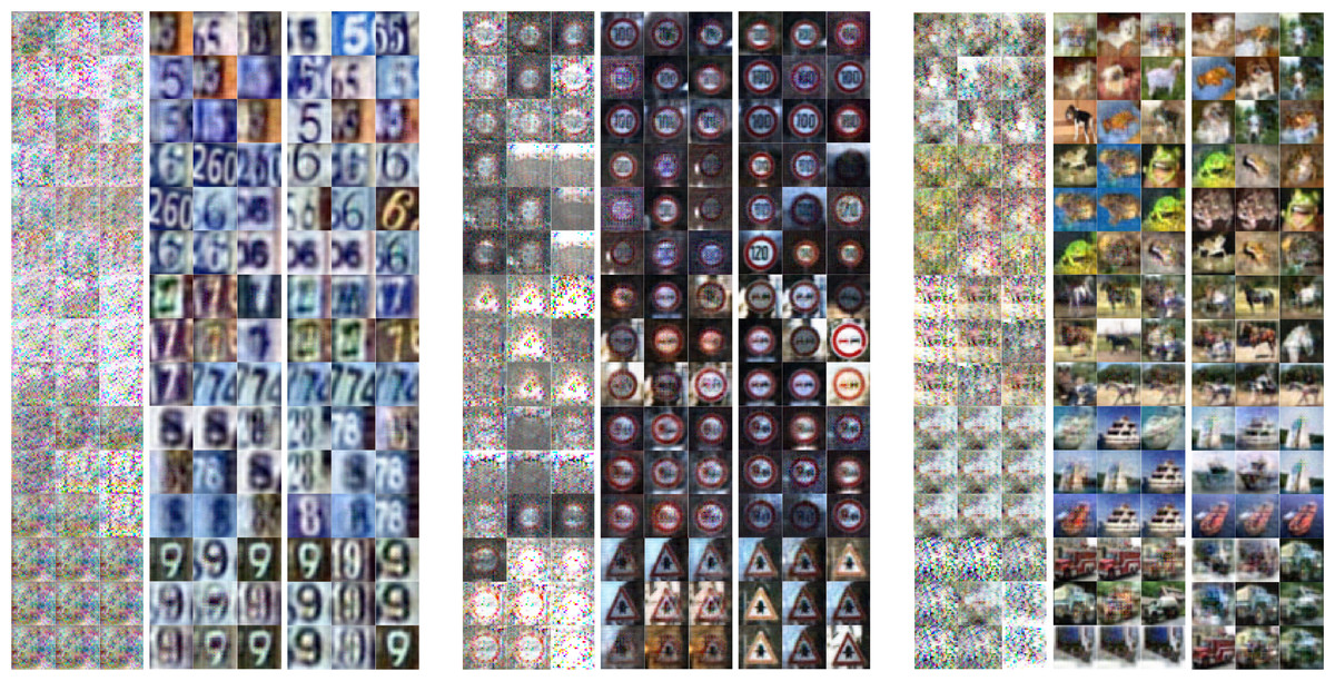
Figure 4: Examples of generated RGB images of the five rarest minority classes from (A) SVHN, (B) GTSRB, and (C) CIFAR10 using BAGAN, DeepSMOTE, and DeepCLSMOTE, respectively (each column showing results from BAGAN, DeepSMOTE, and DeepCLSMOTE).

Download full-size image

DOI: 10.7717/peerj-cs.3461/fig-4

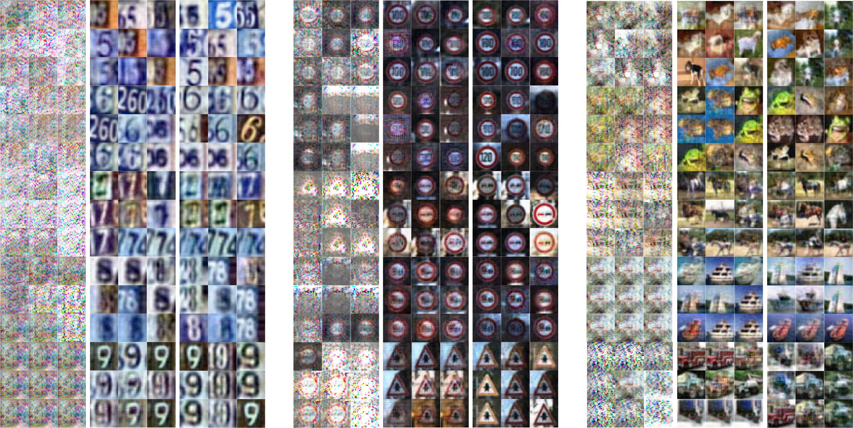
In the case of SVHN, BAGAN produced heavily corrupted images exhibiting limited discernible digit structure, whereas DeepSMOTE yielded samples with improved digit-like forms, although many were blurry or over-smoothed. By contrast, instances synthesized by DeepCLSMOTE were noticeably sharper, better aligned, and more consistent with the visual appearance of real street-view digits.

A similar trend was observed for GTSRB, where traffic sign synthesized by BAGAN were found to lack meaningful structure or color fidelity. Although DeepSMOTE improved the circular and triangular outlines of signs, it frequently failed to replicate internal symbols clearly. DeepCLSMOTE, conversely, was able to produce visually coherent and semantically accurate traffic sign images, with distinctive shapes and internal icons being well-preserved.

For the CIFAR10 dataset, which includes diverse natural and man-made object categories, BAGAN produced noisy and highly abstract instances, lacking distinguishable object features. DeepSMOTE offered modest improvements, but frequently failed to preserve object shapes and background consistency. The most favorable results were regularly obtained using DeepCLSMOTE, which synthesized well-structured images featuring identifiable textures, shapes, and contextual cues across various categories such as animals, ships, and vehicles.

These observations indicate that DeepCLSMOTE achieves superior image quality, realism, and class consistency across evaluated RGB datasets, rendering it more effective for data augmentation under class imbalance scenarios.

Quantitative performance analysis

In addition to a qualitative perspective, this subsection considers the quantitative performance analysis. It presents the overall performance metrics and a statistical comparison of the evaluated methods, detailed in the following sub-subsections.

Overall performance metric

As presented in Table 5, DeepCLSMOTE consistently outperformed the baseline approaches across most datasets and evaluation metrics.

Table 5:

Evaluation of DeepCLSMOTE and reference methods on the balanced test set under a long-tailed recognition setup.

Performance	Approach	Dataset
Performance	Approach	MNIST	FMNIST	EMNIST	SVHN	GTSRB	CIFAR10
Accuracy	Plain	0.8950	0.8767	0.8812	0.8228	0.8204	0.8385
	BAGAN	0.9362	0.9303	0.9235	0.8809	0.8397	0.8586
	DeepSMOTE	0.9537	0.9461	0.9361	0.8871	0.8372	0.8620
	DeepCLSMOTE	0.9581	0.9516	0.9397	0.8874	0.8385	0.8622
Precision	Plain	0.2645	0.2781	0.2363	0.0345	0.0147	0.1193
	BAGAN	0.7217	0.6652	0.6985	0.3377	0.1540	0.3270
	DeepSMOTE	0.8146	0.7469	0.7536	0.4745	0.1058	0.3690
	DeepCLSMOTE	0.8255	0.7829	0.7495	0.4984	0.1730	0.3500
Recall	Plain	0.4752	0.3835	0.4060	0.1139	0.1021	0.1924
	BAGAN	0.6810	0.6513	0.6175	0.4044	0.1983	0.2931
	DeepSMOTE	0.7686	0.7306	0.6804	0.4354	0.1862	0.3100
	DeepCLSMOTE	0.7905	0.7578	0.6984	0.4368	0.1924	0.3111
F1-measure	Plain	0.3383	0.3214	0.2987	0.0527	0.0249	0.1471
	BAGAN	0.7005	0.6581	0.6554	0.3671	0.1676	0.3054
	DeepSMOTE	0.7909	0.7386	0.7151	0.4535	0.1307	0.3367
	DeepCLSMOTE	0.8076	0.7701	0.7230	0.4648	0.1733	0.3291

DOI: 10.7717/peerj-cs.3461/table-5

Note:

Bold values indicate the best performance in each column (dataset).

A notable advantage was observed on simpler datasets. On the MNIST dataset, the highest scores across all evaluated metrics were achieved by DeepCLSMOTE. Similarly, on the Fashion-MNIST dataset, a leading position was maintained by DeepCLSMOTE across all evaluated metrics. Consistent superior performance was also observed for the EMNIST dataset. The performance advantage of DeepCLSMOTE was also discernible on more complex datasets. For SVHN, DeepCLSMOTE outperformed other approaches, particularly in Accuracy and Precision. On GTSRB and CIFAR10, competitive performance was demonstrated.

Compared to DeepSMOTE, identified as the second-best performing method, consistent improvements were shown by DeepCLSMOTE across most metrics. The most significant improvements were observed in Precision and F1-measure, suggesting that DeepCLSMOTE is specifically effective at reducing false positives while maintaining high recall. While DeepCLSMOTE demonstrated overall superiority, it is noted that DeepSMOTE achieved slightly higher performance on specific metrics for certain datasets, such as EMNIST and CIFAR10. This localized difference in performance might be attributed to variations in dataset characteristics; DeepSMOTE’s direct feature space interpolation may occasionally align more favorably with the specific feature distributions or noise patterns present within certain classes within EMNIST and CIFAR10, yielding to a marginal advantage on particular metrics.

The superior overall performance of DeepCLSMOTE is attributable to its unique combination of clustering and synthetic minority oversampling techniques, which effectively addresses class imbalance problems while preserving the structural integrity of the feature space. This approach is particularly valuable for complex image classification tasks where class boundaries may be highly non-linear. When examining the results across varying dataset complexities, it is observed that the performance gap between DeepCLSMOTE and other methods increases as the datasets become more complex, highlighting the robustness of the approach to challenging classification scenarios.

Statistical ranking and comparison

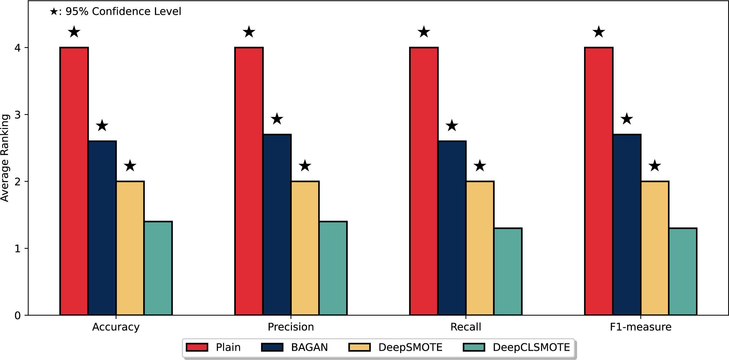
Figure 5 depicts the average ranking of the evaluated methods across the four performance metrics with the entire six datasets: Accuracy, Precision, Recall, and F1-measure. As illustrated, DeepCLSMOTE consistently achieved the best average ranking, with bars approximately 1.3–1.4 across all metrics. This indicates superior performance compared to the other evaluated methods: the simple CNN trained without any data augmentation (Plain), BAGAN, and DeepSMOTE. A Wilcoxon Signed-Rank test (Demšar, 2006) was performed to statistically compare our method against the baseline, analyzing paired performance differences. Stars above the bars denote statistically significant differences at the 95% confidence level ( $p < 0.05$ ), confirming that DeepCLSMOTE’s superior performance represents a statistically significant improvement over all competing methods, not merely a marginal difference. In this ranking system, lower values indicate better performance (Rank 1 being the best). DeepCLSMOTE (green bars) regularly ranked first, followed by DeepSMOTE (yellow bars), then BAGAN (blue bars), and finally Plain (red bars), with approximate average ranks of 2.0, 2.6, and 4.0, respectively. This ranking analysis provides strong statistical evidence of DeepCLSMOTE’s consistent and statistically significant superiority performance across all evaluation metrics relative to all other evaluated methods.

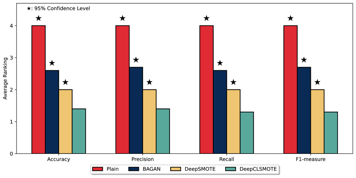
Figure 5: Comparison of mean rankings for DeepCLSMOTE and reference methods, including statistical significance from the Wilcoxon Signed-Rank test.

Download full-size image

DOI: 10.7717/peerj-cs.3461/fig-5

Discussion

The experimental results demonstrate that DeepCLSMOTE significantly enhances the classification performance in imbalanced image datasets. The consistent superiority of the proposed method over BAGAN and the original DeepSMOTE is not merely an incremental improvement; it represents a direct consequence of addressing a core limitation in prior methods. While generative baselines primarily improve performance through data augmentation, DeepCLSMOTE’s key advantage stems from its architectural novelty: the explicit optimization of the autoencoder’s latent space structure.

This optimization is the primary driver of enhanced performance. Although DeepSMOTE effectively utilizes the latent space, it does not actively structure it for class separability. Our method addresses this gap by introducing a composite loss function with two additional terms: the intra-class compactness loss ( $L_{i n t r a}$ ) pulls latent representations of the same class closer to their centroid, while the inter-class separation loss ( $L_{i n t e r}$ ) pushes the centroids of different classes apart. This dual-objective optimization results in a more organized and discriminative latent space, which is the key contributor to improved results. The generated minority samples are not only realistic (as shown in Figs. 3 and 4) but are also synthesized in regions of the feature space that enhance decision boundaries for subsequent classification, leading to the superior accuracy and recall values reported in Table 5.

However, the method exhibits certain limitations that warrant consideration. DeepCLSMOTE may show reduced effectiveness when minority classes have high visual similarity to majority classes, as observed in CIFAR-10 categories where complex natural images with overlapping features yielded more modest improvements. This is exemplified by DeepCLSMOTE’s lower F1-score compared to DeepSMOTE on CIFAR-10, which corresponds to observed image quality limitations in Fig. 4, where the method still struggles to produce clear, detailed images for complex object categories. This suggests potential issues related to insufficient training epochs, model overfitting, or hyperparameter sensitivity for highly complex datasets.

Additional limitations include scenarios where the latent space dimensionality is insufficient to capture intrinsic class complexity, potentially rendering the centroid-based optimization less effective. Furthermore, extreme imbalance ratios beyond our tested $750 : 1$ could lead to unstable centroid calculations, as minority class centroids become overly sensitive to individual samples. The method’s performance also relies on appropriate weighting of the composite loss components ( $λ_{1}, λ_{2}, λ_{3}$ ). While equal weighting $(λ = 1)$ proved effective across our datasets, optimal values likely vary with dataset characteristics and imbalance severity. The inverse distance formulation in $L_{i n t e r}$ , though stabilized with $ε = 1 e - 8$ , may require adjustment for different data distributions.

Conclusions

Training CNNs on imbalanced data sets results in suboptimal performance, particularly with datasets exhibiting extreme imbalance, owing to minority class underrepresentation. To address this challenge, experiments comparing three deep learning models for minority class augmentation, BAGAN, DeepSMOTE, and the proposed DeepCLSMOTE method, were conducted. DeepCLSMOTE consistently outperformed the baseline methods across all evaluation metrics, especially in terms of precision, recall, and F1-score.

Furthermore, qualitative assessments of the synthesized images revealed that DeepCLSMOTE regularly produced instances exhibiting superior visual quality, realism, and class consistency relative to the baseline methods. This superior performance is attributable to DeepCLSMOTE’s unique combination of clustering and synthetic minority oversampling techniques. Specifically, the integration of class centroid information and the optimization of latent space distances prove beneficial for discriminative feature learning, which effectively addresses class imbalance problems while preserving the structural integrity of the feature space. DeepCLSMOTE’s effectiveness in terms of training efficiency and prediction accuracy positions it as a promising approach for imbalanced classification problems.

While this study demonstrates DeepCLSMOTE’s effectiveness, several limitations suggest important directions for future research. Evaluation on naturally imbalanced real-world datasets, extension to other data modalities beyond images, and comprehensive hyperparameter sensitivity analysis would strengthen the method’s validation. Direct comparison with a broader range of imbalanced learning methods beyond our current baselines would provide a more comprehensive performance assessment. Additionally, investigating the relationship between dataset complexity and optimal centroid configurations presents a promising direction for automated parameter selection in diverse application domains.

Supplemental Information

README file for the DeepCLSMOTE code implementation.

Description of the code repository, instructions for running the DeepCLSMOTE implementation, dataset information, requirements, and citation details.

DOI: 10.7717/peerj-cs.3461/supp-1

Download

DeepSMOTE Experiment Python Code.

DOI: 10.7717/peerj-cs.3461/supp-2

Download

[1] Arjovsky M, Chintala S, Bottou L. 2017. Wasserstein generative adversarial networks.

[2] Aubaidan BH, Abdul Kadir R, Lajb MT, Anwar M, Qureshi KN, Taha BA, Ghafoor K. 2025. A review of intelligent data analysis: machine learning approaches for addressing class imbalance in healthcare—challenges and perspectives. Intelligent Data Analysis 29(3)

[3] Buda M, Maki A, Mazurowski MA. 2018. A systematic study of the class imbalance problem in convolutional neural networks. Neural Networks 106(7):249-259

[4] Chawla N, Bowyer K, Hall L, Kegelmeyer W. 2002. Smote: synthetic minority over-sampling technique. Journal of Artificial Intelligence Research 16:321-357

[5] Cohen G, Afshar S, Tapson J, van Schaik A. 2017. EMNIST: an extension of MNIST to handwritten letters.

[6] Dablain D, Krawczyk B, Chawla NV. 2023. Deepsmote: fusing deep learning and smote for imbalanced data. IEEE Transactions on Neural Networks and Learning Systems 34(9):6390-6404

[7] Demšar J. 2006. Statistical comparisons of classifiers over multiple data sets. Journal of Machine Learning Research 7:1-30

[8] Fernández A, García S, Galar M, Prati RC, Krawczyk B, Herrera F. 2018. Learning from imbalanced data sets. Berlin: Springer.

[9] Goodfellow I, Bengio Y, Courville A. 2016. Deep learning. Cambridge, MA: MIT Press.

[10] Goodfellow IJ, Pouget-Abadie J, Mirza M, Xu B, Warde-Farley D, Ozair S, Courville A, Bengio Y. 2014. Generative adversarial nets.

[11] Grandini M, Bagli E, Visani G. 2020. Metrics for multi-class classification: an overview.

[12] Gulrajani I, Ahmed F, Arjovsky M, Dumoulin V. 2017. Improved training of wasserstein gans.

[13] Hassan Pour Zonoozi M, Seydi V. 2022. A survey on adversarial domain adaptation. Neural Processing Letters 55(3):2429-2469

[14] He K, Zhang X, Ren S, Sun J. 2016. Deep residual learning for image recognition.

[15] Heusel M, Ramsauer H, Unterthiner T, Nessler B, Hochreiter S. 2017. Gans trained by a two time-scale update rule converge to a nash equilibrium. Advances in Neural Information Processing Systems 30(1):25-34

[16] Homjandee S, Sinapiromsaran K. 2025. DeepCLSMOTE: deep class-latent synthetic minority oversampling technique.

[17] Ioffe S, Szegedy C. 2015. Batch normalization: accelerating deep network training by reducing internal covariate shift. ArXiv

[18] Johnson JM, Khoshgoftaar TM. 2019. Survey on deep learning with class imbalance. Journal of Big Data 6(1):1-54

[19] Joloudari JH, Marefat A, Nematollahi MA, Oyelere SS, Hussain S. 2023. Effective class-imbalance learning based on smote and convolutional neural networks. Applied Sciences 13(6):4006

[20] Khan AA, Chaudhari O, Chandra R. 2023. A review of ensemble learning and data augmentation models for class imbalanced problems: combination, implementation and evaluation. ArXiv

[21] Kingma DP, Welling M. 2013. Auto-encoding variational bayes. ArXiv

[22] Krawczyk B. 2016. Learning from imbalanced data: open challenges and future directions. Progress in Artificial Intelligence 5(4):221-232

[23] Krizhevsky A. 2009. Learning multiple layers of features from tiny images.

[24] Lauron MLC, Pabico JP. 2016. Improved sampling techniques for learning an imbalanced data set. ArXiv

[25] LeCun Y, Cortes C, Burges CJ. 1998. The mnist database of handwritten digits.

[26] Lin T-Y, Goyal P, Girshick R, He K, Dollár P. 2017. Focal loss for dense object detection.

[27] Mariani G, Scheidegger F, Istrate R, Bekas C, Malossi ACI. 2018. BAGAN: data augmentation with balancing GAN.

[28] Miyato T, Kataoka T, Koyama M, Yoshida Y. 2018. Spectral normalization for generative adversarial networks.

[29] MSE. 2008. Mean squared error. New York, NY: Springer New York. 337-339

[30] Mullick SS, Datta S, Das S. 2019. Generative adversarial minority oversampling.

[31] Netzer Y, Wang T, Coates A, Bissacco A, Wu B, Ng AY. 2011. Reading digits in natural images with unsupervised feature learning.

[32] Paszke A, Gross S, Massa F, Lerer A, Bradbury J, Chanan G, Killeen T, Lin Z, Gimelshein N, Antiga L, Desmaison A, Köpf A, Yang E, DeVito Z, Raison M, Tejani A, Chilamkurthy S, Steiner B, Fang L, Chintala S. 2019. Pytorch: an imperative style, high-performance deep learning library.

[33] Salimans T, Goodfellow I, Zaremba W, Cheung V, Radford A, Chen X. 2016. Improved techniques for training GANs.

[34] Sophia T. 2024. A comprehensive analysis of exploring the efficacy of machine learning algorithms in text, image, and speech analysis. Journal of Electrical Systems 20(2s):910-921

[35] Stallkamp J, Schlipsing M, Salmen J, Stiefelhagen C. 2012. Man vs. computer: benchmarking machine learning algorithms for traffic sign recognition.

[36] Tan J, Wang C, Li B, Li Q, Ouyang W, Yin C, Yan J. 2020. Equalization loss for long-tailed object recognition.

[37] Tang J, Li Y, Hou Z, Fu S, Tian Y. 2024. Robust two-stage instance-level cost-sensitive learning method for class imbalance problem. Knowledge-Based Systems 300(C):112143

[38] Terven J, Cordova-Esparza D-M, Ramirez-Pedraza A, Chávez Urbiola E. 2023. Loss functions and metrics in deep learning. A review.

[39] van den Oord A, Kalchbrenner N, Kavukcuoglu K. 2016. Pixel recurrent neural networks. ArXiv

[40] Xiao H, Rasul K, Vollgraf R. 2017. Fashion-MNIST: a novel image dataset for benchmarking machine learning algorithms. ArXiv