
Masked timesteps in spiking neural networks for efficient time series classification
- Published
- Accepted
- Received
- Academic Editor
- Giulia Cisotto
- Subject Areas
- Data Mining and Machine Learning, Data Science, Neural Networks
- Keywords
- Spiking neural network, Univariate time series classification, Direct encoding
- Copyright
- © 2026 Geng et al.
- Licence
- This is an open access article distributed under the terms of the Creative Commons Attribution License, which permits unrestricted use, distribution, reproduction and adaptation in any medium and for any purpose provided that it is properly attributed. For attribution, the original author(s), title, publication source (PeerJ Computer Science) and either DOI or URL of the article must be cited.
- Cite this article
- 2026. Masked timesteps in spiking neural networks for efficient time series classification. PeerJ Computer Science 12:e3460 https://doi.org/10.7717/peerj-cs.3460
Abstract
Spiking neural networks (SNN) accurately emulate the neurodynamics of biological neurons, theoretically enhancing the processing capabilities for time series data by using spike trains. Existing research, however, has largely remained in an exploratory stage, focusing primarily on the potential of SNNs in time series forecasting rather than classification. Current research on Time Series Classification (TSC) using SNNs often employs complex, pre-trained encoding schemes, relies on reservoir computing, or depends merely on spiking neurons for extracting time series information without fully integrating spiking neurons into the network architecture. Presently, there is a significant gap in SNN research regarding a universally applicable methodology for TSC that balances low temporal complexity with effective, straightforward implementation, trained from scratch, and robust biological plausibility. This article introduces the Masked Timestep SNN (MT-SNN) architecture to selectively mask low neuronal activity timesteps, thereby addressing the entrenched issue of temporal redundancy in SNNs. In addition, our research validates the effectiveness of the direct encoding strategy in SNNs for TSC and proposes the Temporal Adaptive Integrate-and-Fire (TAIF) neuron model, which improves its temporal dynamics through mechanisms of threshold adjustment and fatigue. Our experiments on the UCR Time Series Classification Archive indicate that our approach achieves performance comparable or superior to traditional machine learning and deep learning methods at ultra-low timesteps, obviating the necessity for specialized encoding schemes, preprocessing, or feature engineering. To the best of our knowledge, our approach has achieved the State-of-The-Art (SoTA) spiking result in univariate TSC tasks while maintaining simplicity and biological plausibility, offering a valuable and comprehensive spiking baseline.
Introduction
Time Series Classification (TSC) constitutes a critical area of focus within data mining research, with wide-ranging applications in finance, biomedical signal processing (Gong et al., 2023), and industrial monitoring. The main challenge in TSC is effectively identifying and utilizing significant features in time series data. Traditional approaches, including Dynamic Time Warping (DTW) (Keogh & Ratanamahatana, 2005), Bag-of-SFA-Symbols (BOSS) (Schäfer, 2015), the Collective of Transformation-based Ensembles (COTE) (Bagnall et al., 2015), along with Time Series Bag-of-Features (TSBF) (Baydogan, Runger & Tuv, 2013), serve as foundational techniques. Nevertheless, these methodologies still face difficulties related to high computational costs, lengthy processing durations, complexities in parameter fine-tuning, restricted scalability, and inadequate noise robustness (Bagnall et al., 2017). With the rise of Deep Learning (DL) techniques, DL-based TSC methods address the shortcomings of traditional methods (Ren et al., 2024), classified into generative and discriminative approaches (Fawaz, 2020). Generative models, represented by Autoencoders and Echo State Networks (ESN), contrast with discriminative models, which are subdivided into feature engineering and end-to-end approaches. The latter discriminative methods include Multilayer Perceptrons (MLP), Convolutional Neural Networks (CNN), and hybrid methods. The automated feature extraction capability of DL-based TSC models has simplified data processing tasks compared to traditional TSC methods. However, conventional DL methods for TSC tasks, exemplified by Artificial Neural Networks (ANN), particularly CNNs, confront difficulties involving poor interpretability, high energy consumption, and substantial training data requirements (Li et al., 2023a; Thompson et al., 2021; Zhang et al., 2021; Li et al., 2023b). These constraints limit their adaptability in scenarios where decision transparency and edge computing are crucial.
To overcome the limitations of traditional DL methods in TSC, Spiking Neural Networks (SNN) not only signify a paradigm shift towards systems that mimic biological neural systems but also present a significant advance in terms of their superior biological interpretability and event-driven capabilities (Roy, Jaiswal & Panda, 2019; Deng et al., 2020; Faghihi, Cai & Moustafa, 2022). Notably renowned for these features, SNNs provide a robust alternative with energy efficiency advantages and have been successfully implemented on various neuromorphic hardware platforms such as TrueNorth, Loihi, and SpiNNaker (Akopyan et al., 2015; Davies et al., 2018; Mayr, Hoeppner & Furber, 2019). Additionally, SNNs using unsupervised learning strategies have shown potential in few-shot learning (Yang, Linares-Barranco & Chen, 2022), as they are able to extract discriminative features even with very limited labeled data (Dong et al., 2023). These features make SNNs an ideal solution for TSC tasks.
Currently, SNNs for Time Series Classification (TSC-SNN) architecture have not been widely adopted because spikes are non-differentiable, hindering the use of standard backpropagation algorithms (Wang, Lin & Dang, 2020). Moreover, whether to use spike encoding, the choice of specific encoding strategies, the size of the time window, and the design of the network architecture represent pressing issues that current research must resolve.
Existing TSC-SNN research either relies on complex encoding schemes, necessitates pre-trained encoders or particular data preprocessing, and requires massive parameter tuning to find optimal configurations or extract features by convolutional layers instead of spiking neurons. These methods, which either increase complexity or rely heavily on CNNs, contradict the principles of energy efficiency and biological plausibility.
This article proposes the Masked Timestep Spiking Neural Network (MT-SNN) architecture for univariate TSC tasks. Firstly, we introduce a residual structure with variable timesteps into the TSC-SNN. Compared to previous works and other encoding methods, our approach using direct encoding features ultra-low and variable timesteps, resulting in significant energy efficiency and a reduced need for complex parameter tuning, requiring only the essential timestep settings. Based on variations in spike firing rates within these timesteps, this mechanism selects the timesteps with the highest excitability and transfers them to the subsequent spiking residual block, effectively implementing a form of time-shrunk residual processing. Furthermore, we developed the Temporal Adaptive Integrate-and-Fire (TAIF) model, which adaptively adjusts thresholds based on the current timestep and incorporates a fatigue mechanism to prevent excessive spike firing.
Our architecture has been rigorously evaluated on the UCR Time Series Classification Archive. The results show that the MT-SNN performs better than traditional and DL models in univariate TSC tasks and offers considerable advantages in computational cost and energy consumption by using significantly reduced timesteps. More importantly, the MT-SNN architecture achieves these results using unified TAIF hyperparameter and low timestep settings, without heavy preprocessing, parameter tuning, or special encoding. This advancement in TSC-SNN models makes it a viable option in scenarios where computational resources are limited. The reduced-timestep residual structure of the SNN integrates energy efficiency, adaptability, and high performance, providing a robust baseline for TSC-SNN. To our knowledge, the MT-SNN achieves State-of-The-Art (SoTA) results in TSC-SNN with superior spike rationality.
In this article, we outline our contributions below:
-
1.
Prove that direct encoding, unlike the previous TSC-SNN models that relied on specific encoding, possesses efficiency and simplicity.
-
2.
Propose a novel Residual SNN architecture with variable timesteps, the MT-SNN.
-
3.
Introduce a spiking neuron model with a fatigue mechanism, the TAIF, tailored for TSC tasks.
-
4.
Conduct a comprehensive evaluation of our model on 49 univariate UCR Time Series Classification Archive datasets, achieving SoTA results across all TSC-SNN benchmarks with ultra-low timesteps (up to 5).
The article is organized as follows. ‘Related Work’ provides an exhaustive introduction to previous TSC-SNN methods. ‘Method’ details the specifics of the MT-SNN and TAIF, demonstrating how the masked timesteps and the TAIF fatigue mechanism are implemented. ‘Experiments’ presents detailed experimental results and comparative analyses. ‘Conclusion’ concludes the article and discusses future work.
Related work
This section provides a full review of the research, focusing on two major aspects related to our work: the application of Spiking Neural Networks for Time Series Classification and the existing issues of Temporal Redundancy in SNNs.
Spiking neural networks for time series classification
Regarded as the third generation of neural networks (Maass, 1997), SNNs differ from traditional ML and DL models by emphasizing biological plausibility and energy efficiency. Furthermore, the intrinsic ability of spiking neurons to capture temporal dependencies makes SNNs particularly well-suited for TSC applications in embedded systems, wearable devices, and remote monitoring.
Current methodologies for TSC-SNN are divided into two categories, as illustrated in Fig. 1: reservoir-based methods and deep learning-based methods. The reservoir-based methods include Reservoir Computing (RC) and Echo State Networks (ESN). The deep learning-based methods are further divided into ANN2SNN (ANN to SNN) conversions (Rueckauer et al., 2017) and models trained from scratch (Wu et al., 2019; Sam et al., 2023).
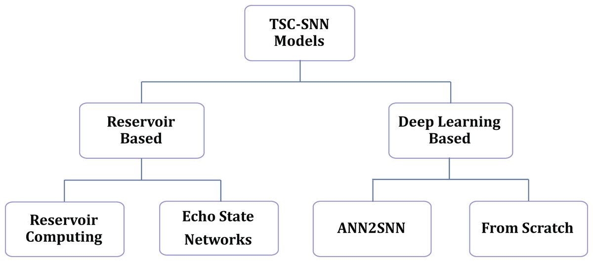
Figure 1: Current methods in TSC-SNNs.
Reservoir computing, specifically ESN, which uses a particular Recurrent Neural Network (RNN) as the reservoir, simplifies training by requiring only adjustments to the weights from the reservoir to the output layer. The dynamic properties of the reservoir efficiently capture the temporal dependencies of the input series. Peng et al. (2024) developed two RC variants for multivariate TSC tasks. Dey et al. (2022) proposed a spike-based reservoir architecture for TSC with two spike-encoding methods to classify vibration time series datasets, and demonstrated that temporal encoding is more effective for TSC than rate encoding. Zhang, Zhu & Li (2018) proposed the Spiking Echo State CNN (SES-CNN), which uses a specialized temporal encoding technique to transform time series data into multichannel spike train signals. The encoded features are extracted using the reservoir computing approach with spiking neurons. The spikes are then converted into 2D mapping images, facilitating classification through a CNN (Zhang, Zhu & Li, 2018).
Although RC, particularly ESN, has advantages in scenarios that are not too complex and require adaptive training, advances in deep learning have overshadowed some of the benefits that RC once offered.
An alternative method to TSC-SNNs uses deep learning techniques, including models converted from ANN as well as those trained from scratch. Yan, Zhou & Wong (2021) introduced a method for energy-efficient ECG classification using an ANN2SNN-based TSC-SNN model. However, the ANN2SNN method requires prolonged timesteps for conversion and imposes constraints such as setting biases to zero and absorbing batch normalization layers (Su et al., 2023). Moreover, the information extraction process is still conducted by well-trained ANNs, which contradicts the biological plausibility of SNNs.
To address this issue, directly-trained SNNs have gained popularity. Fang, Shrestha & Qiu (2020) first applied SNNs to multivariate TSC tasks. They proposed an encoding scheme that converts time series into sparse spatio-temporal spike patterns. Then an iterative SNN model was derived from the Spike Response Model (SRM), enabling the use of Back Propagation Through Time (BPTT) within SNNs (Fang, Shrestha & Qiu, 2020). Gautam & Singh (2020) proposed a hybrid CSNN architecture that uses a differentiable spike generated by the Soft-LIF model to facilitate backpropagation. However, using Soft-LIF compromises the most distinctive feature of SNNs, the binary spike. Gaurav, Stewart & Yi (2023) proposed two TSC-SNN models, inspired by the theories of reservoir computing networks and Legendre Memory Units: one based on RC and another trained using surrogate gradient methods. These models demonstrate the potential of SNNs in temporal data for performance and energy efficiency by nonlinearly decoding the linearly extracted features through spiking neurons (Gaurav, Stewart & Yi, 2023).
Though previous TSC-SNN models have shown some progress, they still encounter certain deficiencies. Some models rely heavily on convolutional layers for feature extraction and consist of only single spike neuron layers, without fully replacing all ReLU units with spiking neurons. Others require complex preprocessing of the original data or the use of sophisticated pre-training encoders. Moreover, some models need multiple sets of reservoir parameters, show limited performance, or have been tested only on specific datasets.
Temporal redundancy in spiking neural networks
Recent studies have pointed out the temporal redundancy in SNNs. Kim et al. (2023) discovered a phenomenon called Temporal Information Concentration (TIC) during the training of SNNs, which indicates the concentration of key information in the early timesteps. As training stabilizes, the sensitivity of the model to new information decreases, leading to great temporal redundancy in later training stages (Kim et al., 2023). Li, Jones & Furber (2023) employed Dynamic Confidence to optimize the latency of inference by dynamically determining when to terminate inference, thereby reducing timesteps.
Several studies are dedicated to overcoming temporal redundancy by reducing timesteps. Li et al. (2024) proposed the Spiking Early-Exit Neural Networks (SEENN), treating the number of timesteps as a variable conditioned on the input samples and using two methods to determine the exit timestep. They also proposed Dynamic Timestep SNN (DT-SNN), which dynamically determines the number of timesteps during inference (Li et al., 2023c). Ding et al. (2024) proposed Shrinking SNN (SSNN), which divides the SNN into multiple stages with progressively shrinking timesteps, and uses a temporal transformer to transform temporal scale of information. Chowdhury, Rathi & Roy (2021b) proposed an Iterative Initialization and Retraining method for SNNs (IIR-SNN) to perform single-shot inference along the temporal axis as the network gradually shrinks in the temporal domain. In particular, they also introduced spatial and temporal pruning and quantization of SNNs, with temporal pruning performed by gradually reducing simulation timesteps during training (Chowdhury, Garg & Roy, 2021a). Suetake et al. (2023) proposed a single-step SNN neuron model, demonstrating its practicality in static image classification using the surrogate gradient method.
The studies above indicate that reducing the number of timesteps effectively optimizes temporal redundancy, indicating considerable potential improvements in edge scenarios that require low latency for TSC. Based on these findings, we propose the MT-SNN architecture, which selectively masks timesteps to ensure that the network efficiently processes temporal information at various stages of training.
Method
In this section, we outline the architecture of MT-SNN, detail the encoding methods employed, and describe the specific network layers. Next, we introduce the implementation of the Masked Timestep, followed by a discussion of the TAIF neuron.
Network structure
Encoding methods
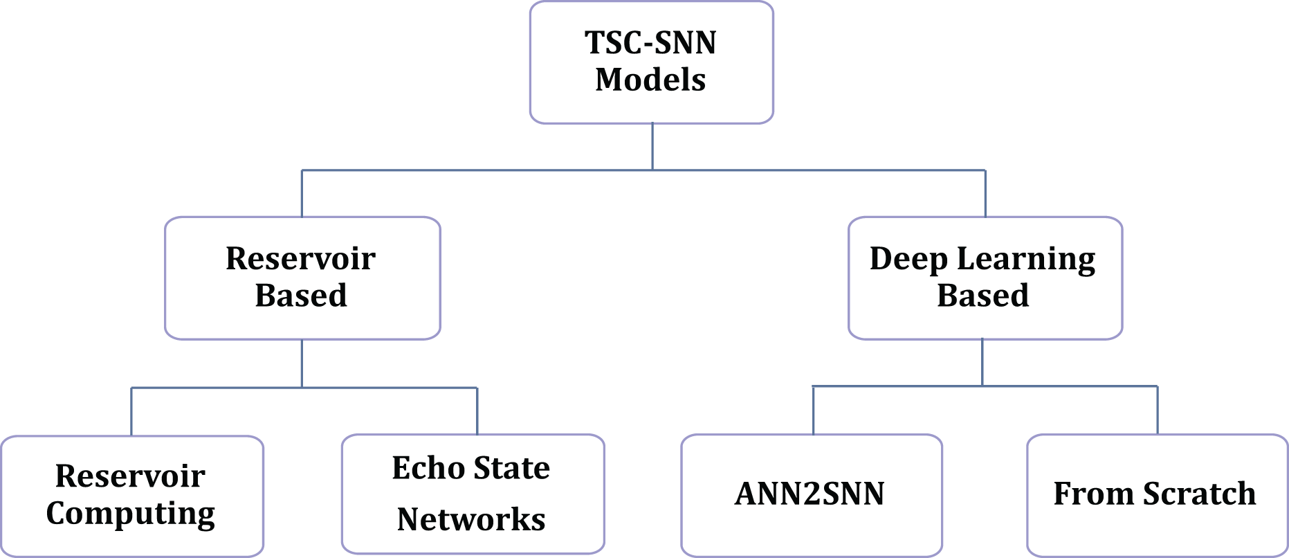
In the context of TSC tasks, a primary challenge is to encode complex and variable time series into spike trains using SNNs without incurring information loss. Rate encoding can approximate the original information without significant loss only in very large timesteps (Kim et al., 2018), but excessive inference time reduces energy efficiency, conflicting with the requirements for low power consumption in TSC tasks. Similarly, latency and temporal encoders face challenges related to parameter tuning or the need for additional pretraining (Chen et al., 2011). Poisson encoding introduces stochasticity by converting input intensities into spike probabilities, which will reduce reproducibility and incur additional computational cost (Rathi & Roy, 2021). Significantly, these methods typically do not achieve high performance. Due to its simplicity, direct encoding has been widely used in tasks such as image recognition (Kim et al., 2022), maintaining the integrity of the original sequence without extensive preprocessing. As one of the most effective methods for classification tasks, direct encoding can even achieve a performance comparable to ANNs (Wu et al., 2019; Zheng et al., 2021). Therefore, in the MT-SNN architecture, direct encoding is used, as illustrated in Fig. 2.
Figure 2: The direct encoding methods for TSC: to reduce the randomness of single neuron firing, direct encoding needs to create an extra time dimension by repeating the original data along the time axis.
The extended time T refers to the timestep. The encoding process from original data to spikes is accomplished by the Convolutional layer, BatchNorm layer, and Spiking Neuron layer.
Spiking residual block
Using direct encoding, the original time series can be transformed into spike trains suitable for an SNN. After encoding, these spike trains are sent to the remainder of the MT-SNN. Recent research strongly supports the superiority of ResNet architectures for univariate TSC tasks. Therefore, we have incorporated the residual network into the architecture. As demonstrated in previous work, we initially replaced all ReLU units in the ResNet architecture with spiking neurons, obtaining a preliminary Spiking Residual Block structure (Han et al., 2022; Fang et al., 2021; Hu et al., 2021; Sengupta et al., 2019).
Structure of Spiking ResNet
To maximize the combination of the advantages of SNN and residual structures, average pooling, which is more consistent with the principles of SNNs, was selected as the pooling method. The classifier structure involves multiple layers including adaptive average pooling, flatten, dropout, and linear layers with spiking layers to implement the spiking mechanism. The general structure of the basic Spiking Resnet is shown in Fig. 3.
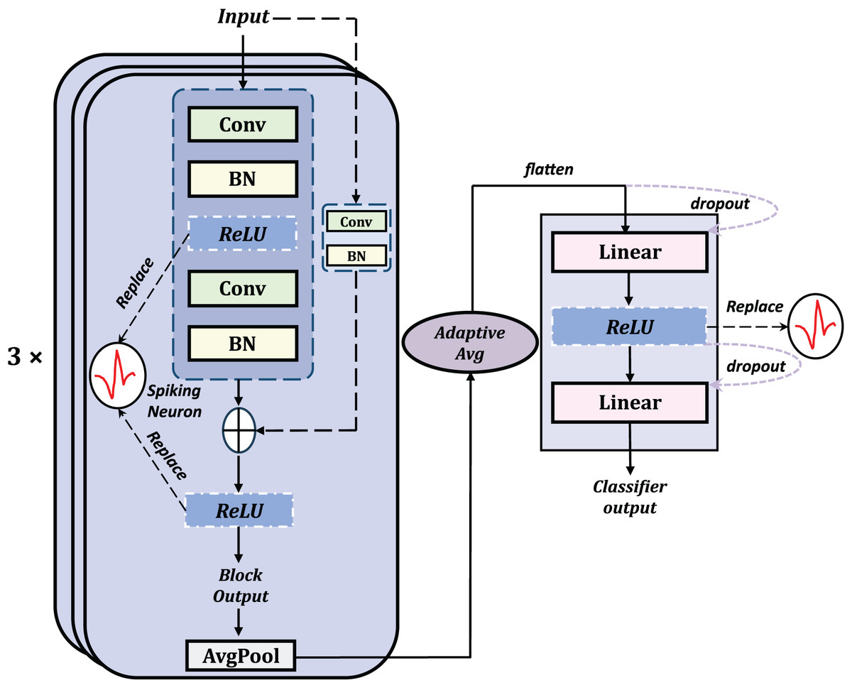
Figure 3: The general structure of the basic residual SNN, obtained by replacing the ReLU with spiking neurons.
Masked timesteps
Although Spiking ResNet, obtained by directly replacing the ReLU activation function, is capable of addressing certain challenges in univariate TSC tasks compared to traditional DL and ML methods, it still encounters temporal redundancy issues. Since spiking neurons are highly correlated with the added time dimension T, in the context of direct encoding, T also represents the number of times the original data are repeated along the time axis. A larger T allows for more refined training but also leads to an increased network depth, resulting in additional computational costs. However, given the wide range of TSC data, selecting an appropriate T for each dataset is not a straightforward task. This is also why we use direct encoding to expand the time dimension rather than directly using the original data length as the time dimension. Inspired by studies on temporal redundancy that indicate that only a subset of the timesteps is significant during the training process of SNNs, we apply a masking technique to the timesteps in the Spiking Residual Blocks, thereby retaining only those timesteps that are important.
Univariate TSC modeling
Generally, the raw time series, denoted as , comprises a single-channel sequence with a length of L and is associated with a class label . Univariate TSC tasks involve assigning class labels to sequences of time series data using a supervised classifier. To make suitable for Spiking Residual Block, the input must be transfromed into , where T is the number of timesteps, B is the batch size, C is the number of channels, and L is the length of each univariate time series.
Spiking neuron integration
The spiking neuron layer, , is used to replace the ReLU activation in the residual block. Subsequently, the direct encoded input, X, is fed into the Spike Encoder to generate spikes, .
This process is outlined as follows:
(1)
Following this, the is sent to the remaining parts of Block, obtaining the output for each timestep.
Temporal selection
In order to reduce temporal redundancy, we apply the mask M to selectively disable certain unimportant timesteps. The criterion for measuring their contribution is the firing frequency FR. The temporal reduction between Spiking Residual Blocks can be seen in Fig. 4. According to the Hebbian learning rule, a greater number of spikes indicates more substantial learning, as the frequency of these spikes characterizes the intensity of the learning process.
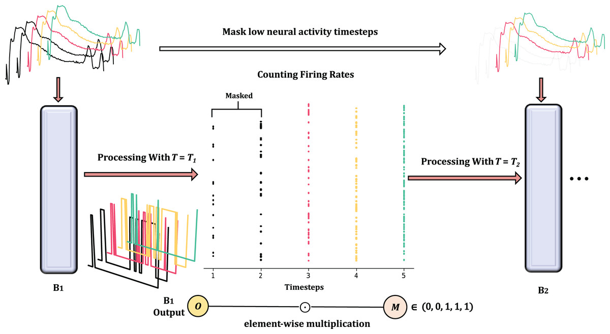
Figure 4: The overview of masked timestep in Spiking Residual Blocks, the more detailed processing is in Algorithm 1.
In the figure, and as the first 2 timesteps are masked due to low neural activaty.
To calculate FR, we concatenate outputs along the time dimension to obtain the concat output .
Due to the binary nature of spiking neurons, the firing rate (FR) at timestep is obtained by summing across the channel and feature dimensions. This can be expressed as follows:
(2)
In this way, is a scalar per timestep and per sample; for a batch of size B, forms a matrix of size . The mask M is then applied to the output of each timestep:
(3) with broadcasting along the dimensions, where denotes element-wise multiplication.
Afterward, the network retains the timesteps with high firing rates based on the predefined number of timesteps to be kept. The output, , is then fed into the next Spiking Residual Block.
The general details of applying the masked timestep method are depicted in Algorithm 1.
| Parameters: |
| Bi: The i-th Spiking Residual Block, |
| N: Total number of Spiking Residual Blocks |
| Ti: Number of current timesteps processed by Bi |
| Tn: Number of next timesteps processed by |
| M: Binary mask indicating active timesteps |
| FR: Firing rates of the temporal dimension, defined as the average number of spikes per unit time |
| Input: |
| x : Input time series |
| Output: |
| : Final classification output |
| 1: Reshape input x to in order to fit direct encoding |
| 2: Initialize an all True mask M with the same shape as X |
| 3: Set initial Ti as the number of timesteps for the first block |
| 4: for Bi; do |
| 5: Get next number of timesteps Tn for |
| 6: if Tn is None then |
| 7: Process X without temporal masking |
| 8: else |
| 9: Clone current mask M to create |
| 10: for do |
| 11: Compute block output Ot using the Spiking Residual Block Bi |
| 12: Apply mask to Ot |
| 13: end for |
| 14: Compute firing rates FR based on the block outputs |
| 15: Sort timesteps in Ti according to FR |
| 16: Select top Tn timesteps: |
| 17: Create new mask M such that , others = 0 |
| 18: end if |
| 19: Pass masked output through avgpooling layer |
| 20: Update Ti with Tn for the next block |
| 21: end for |
| 22: Pass the final output through the classifier layers |
| 23: Average the output yt across the time dimension to get the final classification output |
| 24: Return |
TAIF neuron
In this section, the proposed Temporal Adaptive Integrate-and-Fire (TAIF) neuron is detailed.
Overview of spiking neurons
The introduction of spiking neuron models has been a significant advancement in neural network fields, providing a more accurate representation of the information processing mechanisms in biological neurons. The activities of all spiking neurons can be simply summarized into the following three aspects:
(4)
(5)
(6) where is the Heaviside function.
Equations (4) and (5) represent the charge and fire behaviors of neurons, respectively, while reset behavior can be categorized into two types: soft and hard, as shown in Eqs. (7) and (8).
(7)
(8)
In the aforementioned equations, the subscript denotes time, denotes input, denotes the membrane potential after charging and before the spike fires, and denotes the membrane potential after a spike has been fired. is the function used to update the state of the neuron. In TSC tasks, since the sequences are temporally continuous, the historical states of the neurons should not be reset to . Therefore, the TAIF neuron model uses soft reset.
Training strategy
One major challenge in training SNNs is the non-differentiability of spikes. In this article, we choose to use the surrogate gradient method to directly train SNNs with the BPTT method, using a differentiable surrogate function to replace during backpropagation (Neftci, Mostafa & Zenke, 2019; Lee, Delbruck & Pfeiffer, 2016). The surrogate gradient technique performs excellently, allowing for easy integration into modern deep learning frameworks and requiring neither a large number of timesteps nor extensive tuning.
In MT-SNN, for all spiking neurons, we approximate the derivative of as
(9) where is the derivative of
(10)
Here, is a hyperparameter used to control the shape of the function. To prevent vanishing or exploding gradients, we use , which ensures that the maximum value of the gradient of the surrogate function is 1. The specific shape of the surrogate function is illustrated in Fig. 5.
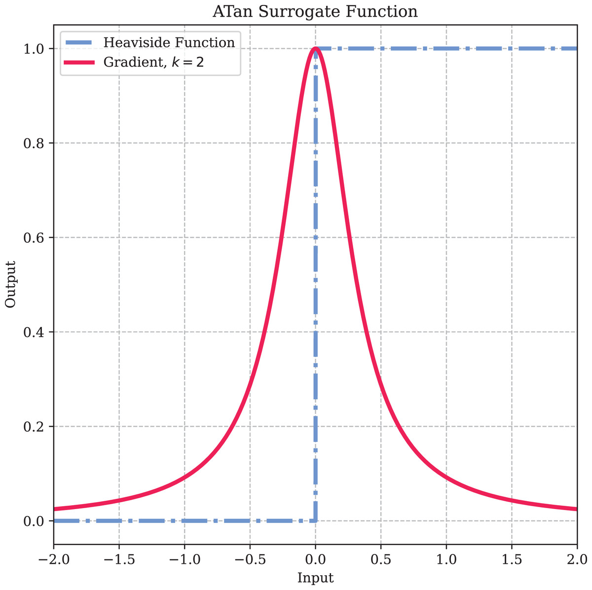
Figure 5: The surrogate gradient method.
In SNNs, commonly used spiking neurons include IF neurons and Leaky Integrate-and-Fire (LIF) neurons (Abbott, 1999). However, in TSC tasks, the leakage characteristics of LIF neurons often lead to suboptimal performance compared to IF neurons, making the IF neuron more suitable. However, the reduction in time steps in MT-SNN causes standard IF neurons to lack awareness of this change, leading to redundant processing steps. To address this issue, we propose an improved IF neuron, termed the Temporal Adaptive Integrate-and-Fire (TAIF) neuron, inspired by biological neurons. We introduce a fatigue mechanism into IF neurons, making them more prone to fatigue in the early training stages with long timesteps, while more excitable in the later stages of short timesteps. This behavior aligns with the TIC phenomenon and optimizes the temporal information distribution, enhancing their robustness and performance.
The charge function of the TAIF neuron is the same with standard IF neuron:
(11)
In simulation, we use discrete difference equations to approximate continuous differential equations:
(12)
To ensure the simplicity of IF neurons, the improvements in TAIF focus on the fire and reset behaviors. First, the TAIF charges according to the charging Eq. (12). Then, it determines whether has reached the threshold potential . If exceeds , a spike fired and the fatigue value increases by and without recovery behavior, where denotes the fatigue growth factor. If does not reach , the neuron does not fire spike, and the fatigue value decreases by to simulate fatigue recovery behavior, where denotes the fatigue recovery rate. The accumulated fatigue value then directly affects the threshold potential . The current timestep T is used as a coefficient for , allowing the model to capture temporal changes. The update process of TAIF can be seen in Algorithm 2.
| Input: Output from convolutional and batch normalization layers at timestep t, |
| Output: Spike train |
| 1: Initialize and |
| 2: for to T do |
| 3: Neuron Charge: |
| 4: Update membrane potential Ht based on input |
| 5: if then |
| 6: Neuron Fire: |
| 7: |
| 8: Fatigue factor update: |
| 9: Neuron Reset: |
| 10: |
| 11: else |
| 12: No spike fired |
| 13: |
| 14: Decrease fatigue factor Ft and ensure it does not fall below 0: |
| 15: end if |
| 16: Update threshold potential: |
| 17: end for |
| 18: Return output spike train |
In this way, we can directly train the spiking neuron layers using the BPTT method.
First, we define the FPTT function as follows:
(13)
So the backward function is:
(14)
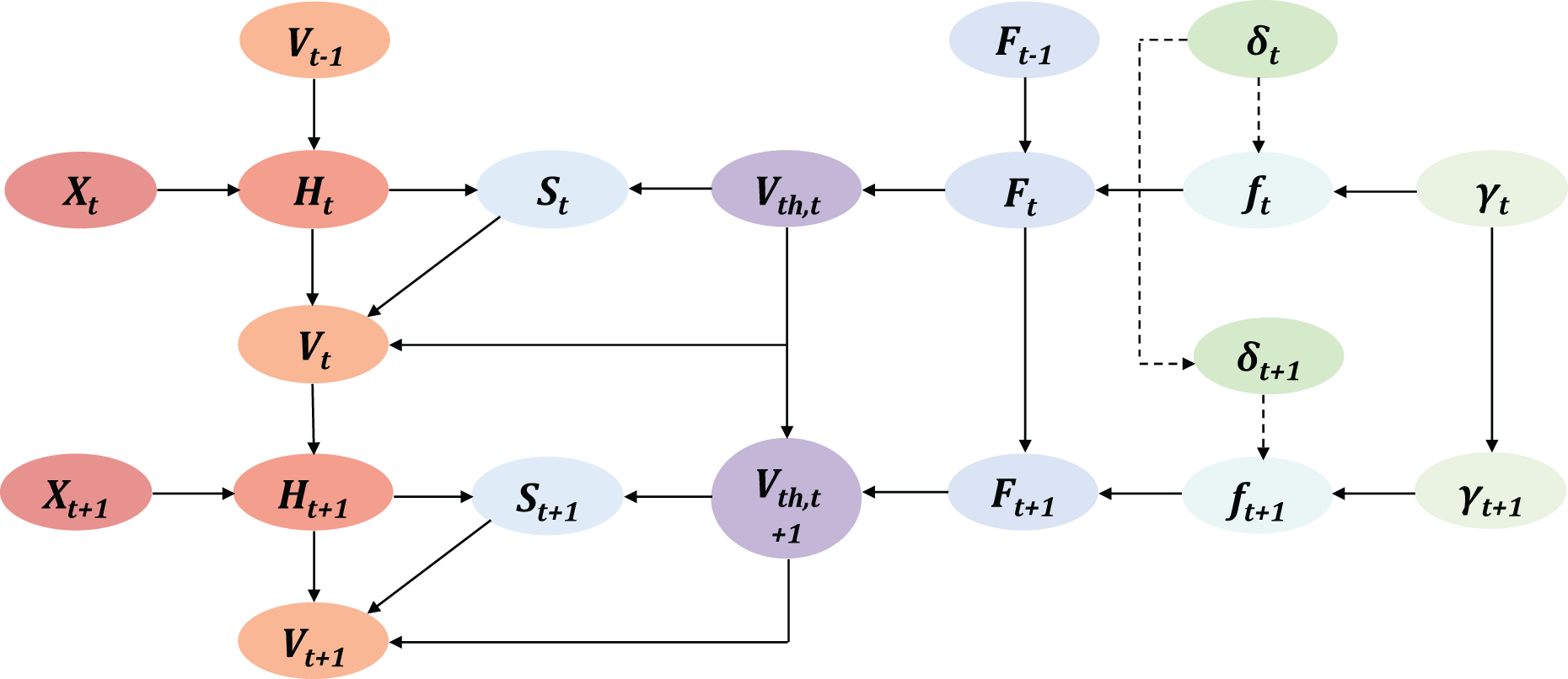
Based on the TAIF update process, the computation graph is shown in Fig. 6.
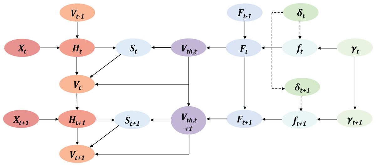
Figure 6: The computation graph of TAIF in time dimension, the dotted line represents the situation when the neuron is not firing.
The gradient of TAIF is as follows:
(15)
(16)
While = 0:
(17)
The gradient of the loss function L to the threshold voltage at time is:
(18) where:
(19)
Therefore, the complete formula is:
(20)
So we can calculate the gradients for :
(21)
Experiments
Unlike previous TSC-SNN works that were tested only on specific datasets, we conducted a comprehensive comparison using 49 univariate UCR datasets evaluated in related traditional, DL and TSC-SNN studies. Our model achieved SoTA performance compared to previous SNN models.
Parameter settings
The CSNN architecture consists of three stacked Spiking Residual Blocks followed by a classifier. Each SRB comprises two convolutional layers, batch normalization, and TAIF neuron layers. The output of each SRB is passed through an average pooling layer for downsampling. The detailed settings of the network architecture are in Table 1.
| Layer | Description |
|---|---|
| SRB with timestep and kernel size | |
| SRB with timestep and kernel size | |
| SRB with timestep and kernel size | |
| 1D average pooling layer with kernel size | |
| Adaptive 1D average pooling with output 4 | |
| Flatten layer | |
| Dropout layer with probability | |
| Linear (fully-connected) layer | |
| Integrate-and-Fire neuron layer |
In all our tests, we used the same network structure to demonstrate the versatility of MT-SNN, and employed the same seed to ensure reproducibility. For optimization, we used Adam Optimizer with CyclicLR Scheduler (Kingma & Ba, 2017). The learning rate for Adam was set to 0.001. To encourage correct firing of neurons while silencing the others, we use MSE as the loss function.
To validate the generalizability of the MT-SNN, we adjusted only the batch size for different datasets, making it the sole hyperparameter that required adjustment, an advantage not achieved in previous works. In practical applications, one only needs to set the desired timestep reduction number. To further demonstrate the effectiveness of the proposed method, we used two timestep reduction settings (maximum timesteps of 5 or 3) in our evaluation. The evaluation results indicate that the MT-SNN achieves remarkable performance even under ultra-low timesteps (3-2-1). Detailed settings can be found in Table 2.
| Datasets | Classes | Batch | Timestep reduction |
|---|---|---|---|
| Adiac | 37 | 256 | 5-3-1 |
| Beef | 5 | 16 | 3-2-1 |
| CBF | 3 | 16 | 3-2-1 |
| ChlorineCon | 3 | 64 | 5-3-1 |
| CinCECGTorso | 4 | 40 | 5-3-1 |
| Coffee | 2 | 28 | 3-2-1 |
| CricketX | 12 | 256 | 5-3-1 |
| CricketY | 12 | 256 | 5-3-1 |
| CricketZ | 12 | 256 | 5-3-1 |
| DiatomSizeR | 4 | 16 | 5-3-1 |
| Earthquakes | 2 | 64 | 5-3-1 |
| ECG200 | 2 | 64 | 5-3-1 |
| ECG5000 | 5 | 16 | 3-2-1 |
| ECGFiveDays | 2 | 64 | 3-2-1 |
| FaceAll | 14 | 64 | 3-2-1 |
| FaceFour | 4 | 24 | 3-2-1 |
| FacesUCR | 14 | 200 | 5-3-1 |
| FiftyWords | 50 | 256 | 5-3-1 |
| Fish | 7 | 32 | 3-2-1 |
| FordA | 2 | 50 | 5-3-1 |
| FordB | 2 | 50 | 5-3-1 |
| GunPoint | 2 | 50 | 3-2-1 |
| Haptics | 5 | 64 | 3-2-1 |
| InlineSkate | 7 | 16 | 5-3-1 |
| ItalyPower | 2 | 64 | 3-2-1 |
| Lightning2 | 2 | 32 | 3-2-1 |
| Lightning7 | 7 | 32 | 3-2-1 |
| MALLAT | 8 | 55 | 3-2-1 |
| MedicalImages | 10 | 381 | 3-2-1 |
| MoteStrain | 2 | 20 | 3-2-1 |
| NonInvThorax1 | 42 | 32 | 3-2-1 |
| NonInvThorax2 | 42 | 32 | 3-2-1 |
| OliveOil | 4 | 30 | 3-2-1 |
| OSULeaf | 6 | 128 | 3-2-1 |
| SonyAIBO | 2 | 20 | 3-2-1 |
| SonyAIBOII | 2 | 20 | 3-2-1 |
| StarLightCurves | 3 | 64 | 3-2-1 |
| SwedishLeaf | 15 | 128 | 3-2-1 |
| Symbols | 6 | 25 | 3-2-1 |
| SyntheticControl | 6 | 16 | 3-2-1 |
| Trace | 4 | 16 | 3-2-1 |
| TwoLeadECG | 2 | 16 | 3-2-1 |
| TwoPatterns | 4 | 16 | 3-2-1 |
| UWaveX | 8 | 32 | 3-2-1 |
| UWaveY | 8 | 32 | 3-2-1 |
| UWaveZ | 8 | 32 | 3-2-1 |
| Wafer | 2 | 128 | 3-2-1 |
| WordSynonyms | 25 | 256 | 3-2-1 |
| Yoga | 2 | 256 | 3-2-1 |
Our experiments were conducted using an RTX 4090 GPU and an Intel Core I9-14900K processor, operating under Ubuntu 22.04 LTS. The experimental framework used the SpikingJelly library (version 0.0.0.0.15) (Fang et al., 2023) and PyTorch (version 2.0.1) (Paszke et al., 2019). The version of the graphics card driver is 535.86.05, with CUDA 12.1.
Ablation study
In this section, detailed ablation experiments are conducted to demonstrate the effectiveness of the proposed modules. Here, MT-SNN-TAIF ( - - ) represents the network using Masked Timestep and TAIF, with timesteps reduced from to to . MT-SNN-IF ( - - ) is the counterpart using IF neurons. SNN (T) denotes the standard SNN network without Masked Timestep and TAIF, with a fixed timestep T. The models mentioned above use the direct encoding method.
Three representative datasets were selected: Adiac, FordB, and DiatomSizeR, with , , , and to represent timesteps ranging from very short to very long. The results are shown in Table 3. MT-SNN was not tested at and because there are insufficient timesteps to apply reduction with only one timestep. When , selecting appropriate timesteps becomes both complex and unnecessary, as most timesteps are redundant. Additionally, MT-SNN is specifically designed for low timestep settings, making tests at high timesteps misaligned with the intended design focus.
| Dataset | Model | T = 1 | T = 3 | T = 5 | T = 20 |
|---|---|---|---|---|---|
| Adiac | SNN | 82.81% | 85.50% | 85.55% | 87.11% |
| MT-SNN-IF | – | 85.55% | 87.50% | – | |
| MT-SNN-TAIF | – | 85.94% | 88.28% | – | |
| FordB | SNN | 82.37% | 82.37% | 82.75% | 83.37% |
| MT-SNN-IF | – | 83.00% | 84.25% | – | |
| MT-SNN-TAIF | – | 83.75% | 85.50% | – | |
| DiatomSizeR | SNN | 96.09% | 96.05% | 94.41% | 96.88% |
| MT-SNN-IF | – | 95.72% | 93.09% | – | |
| MT-SNN-TAIF | – | 96.71% | 98.68% | – |
From Table 3, it can be observed that if an appropriate timestep is selected, direct-encoding SNNs can be highly competitive, demonstrating the simplicity and efficiency of direct encoding compared to rate encoding or latency encoding in classification tasks. This observation is consistent with the results in image classification tasks. However, the performance of direct encoding method is highly related to the timesteps. In the shortest timestep, the model exhibits the lowest accuracy. As the timestep increases, the accuracy improves, but there is a point of diminishing returns where excessively long timesteps can actually degrade performance and bring extra computation cost. This indicates that the baseline model, SNN, has considerable temporal redundancy and that selecting an appropriate timestep is crucial for optimal performance. Our proposed Masked Timestep method requires only an appropriate number of timesteps. As shown in the table, the timesteps for MT-SNN, demonstrating that only five maximum timesteps can surpass the performance of SNN at 20 timesteps. However, the use of the MT method is limited by IF neurons. In the DiatomSizeR dataset, the standalone MT method even leads to a performance decline. By introducing TAIF neurons, MT-SNN consistently outperforms SNN with longer timesteps, even at ultra-low timesteps. Figure 7 indicates that in the first 100 epochs, all models except SNN (T = 20) have converged, showing that direct encoding requires more time to converge in large timesteps and exhibits noticeable oscillations in the early stages of training. As the training progresses, MT-SNN-TAIF shows a smoother and higher test accuracy compared to its counterparts at T = 3 and T = 5. This indicates that the MT-SNN-TAIF architecture has a stronger learning capacity and benefits more from additional training epochs. These results strongly demonstrate the synergistic effect of the MT method with TAIF and verify its superiority in low timestep configurations.
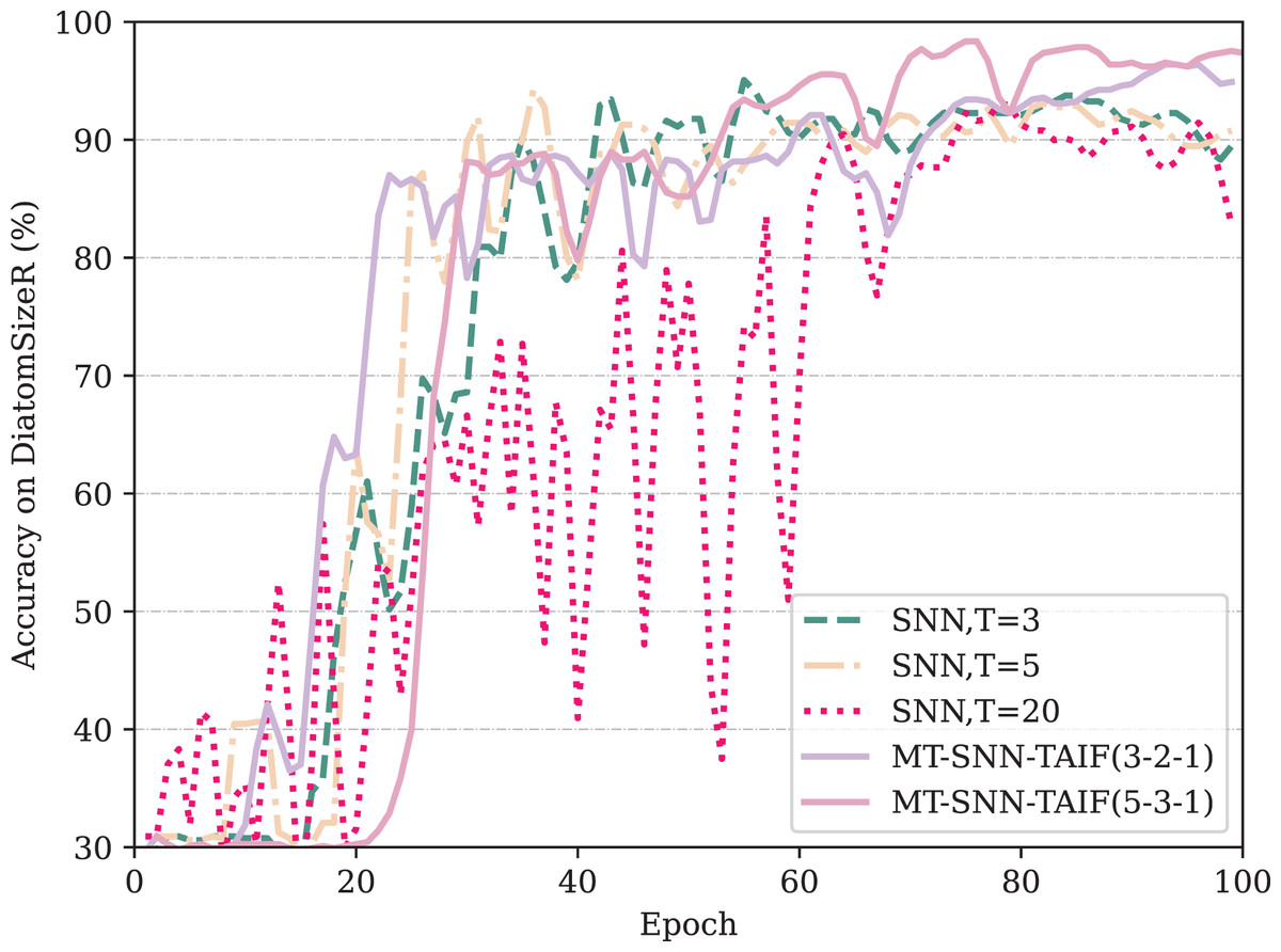
Figure 7: The test accuracy on DiatomSizeR dataset over the first 100 epochs.
Comparison with previous work
In this section, we evaluate our proposed method on a total of 49 UCR univariate time series datasets. Regarding the evaluation metrics, we adopt the Mean Per-Class Error (MPCE) proposed by Wang, Yan & Oates (2017) to evaluate model classification performance in multiple datasets. For a model , dataset pool , class labels , and error rates , we have:
(22)
(23)
Here, indexes datasets, and indexes models. MPCE reflects the expected error rate for a single class across all datasets. Considering the number of classes, MPCE is a robust baseline criterion. We also present the average arithmetic ranking, the average geometric ranking and the critical difference diagram between MT-SNN and other methods.
Comparison with non-SNN work
• Comparison with traditional methods:
For traditional methods, we selected seven representative methods. DTW refers to 1NN-DTW, which is a simple and effective distance-based method but has a high computational cost and is sensitive to noise. BOSS is a dictionary-based method that handles symbolic representations well but relies on parameter settings. COTE and BOSSVS are ensemble models that combine multiple classifiers while consuming many computational resources. PROP combines 11 classifiers based on various elastic distance measures. SE1 is also an ensemble model based on discriminative shapelets. TSBF is a feature-based method that captures local patterns effectively but is influenced by segmentation and feature extraction strategies. The overall evaluation results and the CD-diagram can be seen in Table 4 and Fig. 8, respectively. Compared to traditional methods, the MT-SNN, an end-to-end, from scratch trained approach that does not require extra feature engineering, achieved the best performance. Additionally, MT-SNN does not require extensive hyperparameter tuning and exhibts tolerance to noise and the ability to learn under constrained conditions.
• Comparison with DL-based methods: In DL-based methods, we adopt three baselines proposed by Wang, Yan & Oates (2017): the MLP, FCN, ResNet, and MCNN proposed by Cui, Chen & Chen (2016). The MLP consists of three fully connected layers with 500 neurons each, utilizing ReLU activation functions and dropout; the softmax function is employed for final classification. The FCN comprises three convolutional layers with 128, 256, and 128 filters, respectively. Each layer is followed by batch normalization (BN) and ReLU activation functions, and the global pooling layer aggregates the feature maps into a single vector. The output layer employs a softmax activation function for classification. The ResNet uses three stacked residual blocks with filters of 64, 128, and 128. The classifier consists of a global average pooling layer followed by a softmax function. The MCNN method uses downsampling, skip sampling, and sliding windows to preprocess the data for multi-scale settings, leading to significant preprocessing work and data augmentation. The overall evaluation results and the CD-diagram are presented in Table 5 and Fig. 9, respectively. Among the four models, the FCN achieves the best performance. The ResNet performs slightly worse due to its tendency to overfit. However, the MT-SNN achieves the best results with a structure similar to the ResNet, indicating that the masked timestep spiking residual block has a better generalization capacity, more reasonable biological plausibility and does not require extensive preprocessing and data augmentation used in MCNN.
| Err rate | DTW | COTE | BOSSVS | PROP | BOSS | SE1 | TSBF | MT-SNN (Ours) |
|---|---|---|---|---|---|---|---|---|
| Adiac | 0.396 | 0.233 | 0.302 | 0.353 | 0.220 | 0.373 | 0.245 | 0.117 |
| Beef | 0.367 | 0.133 | 0.267 | 0.367 | 0.200 | 0.133 | 0.287 | 0.125 |
| CBF | 0.003 | 0.001 | 0.001 | 0.002 | 0 | 0.010 | 0.009 | 0 |
| ChlorineCon | 0.352 | 0.314 | 0.345 | 0.360 | 0.340 | 0.312 | 0.336 | 0.196 |
| CinCECGTorso | 0.349 | 0.064 | 0.130 | 0.062 | 0.125 | 0.021 | 0.262 | 0.040 |
| Coffee | 0 | 0 | 0.036 | 0 | 0 | 0 | 0.004 | 0 |
| CricketX | 0.246 | 0.154 | 0.346 | 0.203 | 0.259 | 0.297 | 0.278 | 0.250 |
| CricketY | 0.256 | 0.167 | 0.328 | 0.156 | 0.208 | 0.326 | 0.259 | 0.185 |
| CricketZ | 0.246 | 0.128 | 0.313 | 0.156 | 0.246 | 0.277 | 0.263 | 0.177 |
| DiatomSizeR | 0.033 | 0.082 | 0.036 | 0.059 | 0.046 | 0.069 | 0.126 | 0.013 |
| ECGFiveDays | 0.232 | 0 | 0 | 0.178 | 0 | 0.055 | 0.183 | 0.065 |
| FaceAll | 0.192 | 0.105 | 0.241 | 0.152 | 0.210 | 0.247 | 0.234 | 0.174 |
| FaceFour | 0.170 | 0.091 | 0.034 | 0.091 | 0 | 0.034 | 0.051 | 0 |
| FacesUCR | 0.095 | 0.057 | 0.103 | 0.063 | 0.042 | 0.079 | 0.090 | 0.066 |
| FiftyWords | 0.310 | 0.191 | 0.367 | 0.18 | 0.301 | 0.288 | 0.209 | 0.184 |
| Fish | 0.177 | 0.029 | 0.017 | 0.034 | 0.011 | 0.057 | 0.080 | 0.038 |
| GunPoint | 0.093 | 0.007 | 0 | 0.007 | 0 | 0.060 | 0.011 | 0 |
| Haptics | 0.623 | 0.488 | 0.584 | 0.584 | 0.536 | 0.607 | 0.488 | 0.500 |
| InlineSkate | 0.616 | 0.551 | 0.573 | 0.567 | 0.511 | 0.653 | 0.603 | 0.720 |
| ItalyPower | 0.050 | 0.036 | 0.086 | 0.039 | 0.053 | 0.053 | 0.096 | 0.026 |
| Lightning2 | 0.131 | 0.164 | 0.262 | 0.115 | 0.148 | 0.098 | 0.257 | 0.094 |
| Lightning7 | 0.274 | 0.247 | 0.288 | 0.233 | 0.342 | 0.274 | 0.262 | 0.094 |
| MALLAT | 0.066 | 0.036 | 0.064 | 0.050 | 0.058 | 0.092 | 0.037 | 0.042 |
| MedicalImages | 0.263 | 0.258 | 0.474 | 0.245 | 0.288 | 0.305 | 0.269 | 0.228 |
| MoteStrain | 0.165 | 0.085 | 0.115 | 0.114 | 0.073 | 0.113 | 0.135 | 0.073 |
| NonInvThorax1 | 0.210 | 0.093 | 0.169 | 0.178 | 0.161 | 0.174 | 0.138 | 0.098 |
| NonInvThorax2 | 0.135 | 0.073 | 0.118 | 0.112 | 0.101 | 0.118 | 0.130 | 0.073 |
| OliveOil | 0.167 | 0.100 | 0.133 | 0.133 | 0.100 | 0.133 | 0.090 | 0.033 |
| OSULeaf | 0.409 | 0.145 | 0.074 | 0.194 | 0.012 | 0.273 | 0.329 | 0.102 |
| SonyAIBO | 0.275 | 0.146 | 0.265 | 0.293 | 0.321 | 0.238 | 0.175 | 0.018 |
| SonyAIBOII | 0.169 | 0.076 | 0.188 | 0.124 | 0.098 | 0.066 | 0.196 | 0.083 |
| StarLightCurves | 0.093 | 0.031 | 0.096 | 0.079 | 0.021 | 0.093 | 0.022 | 0.022 |
| SwedishLeaf | 0.208 | 0.046 | 0.141 | 0.085 | 0.072 | 0.120 | 0.075 | 0.082 |
| Symbols | 0.050 | 0.046 | 0.029 | 0.049 | 0.032 | 0.083 | 0.034 | 0.033 |
| SyntheticControl | 0.007 | 0 | 0.040 | 0.010 | 0.030 | 0.033 | 0.008 | 0 |
| Trace | 0 | 0.010 | 0 | 0.010 | 0 | 0.050 | 0.020 | 0 |
| TwoLeadECG | 0 | 0.015 | 0.015 | 0 | 0.004 | 0.029 | 0.001 | 0 |
| TwoPatterns | 0.096 | 0 | 0.001 | 0.067 | 0.016 | 0.048 | 0.046 | 0 |
| UWaveX | 0.272 | 0.196 | 0.270 | 0.199 | 0.241 | 0.248 | 0.164 | 0.196 |
| UWaveY | 0.366 | 0.267 | 0.364 | 0.283 | 0.313 | 0.322 | 0.249 | 0.272 |
| UWaveZ | 0.342 | 0.265 | 0.336 | 0.290 | 0.312 | 0.346 | 0.217 | 0.232 |
| Wafer | 0.020 | 0.001 | 0.001 | 0.003 | 0.001 | 0.002 | 0.004 | 0 |
| WordSynonyms | 0.351 | 0.266 | 0.439 | 0.226 | 0.345 | 0.357 | 0.302 | 0.315 |
| Yoga | 0.164 | 0.113 | 0.169 | 0.121 | 0.081 | 0.159 | 0.149 | 0.145 |
| Win | 3 | 12 | 4 | 5 | 13 | 3 | 4 | 21 |
| AVG arithmetic ranking | 6.14 | 2.68 | 5.52 | 4.18 | 3.50 | 5.59 | 4.98 | 2.23 |
| AVG geometric ranking | 5.48 | 2.25 | 4.76 | 3.63 | 2.80 | 4.98 | 4.34 | 1.83 |
| MPCE | 0.0397 | 0.0226 | 0.0330 | 0.0304 | 0.0256 | 0.0302 | 0.0335 | 0.0188 |
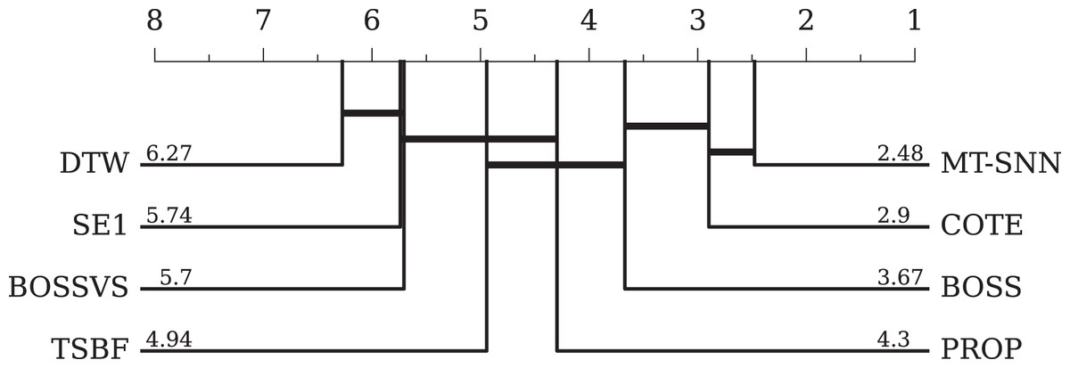
Figure 8: The critical difference diagram between MT-SNN and traditional methods.
| Err rate | MCNN (Cui, Chen & Chen, 2016) | MLP (Wang, Yan & Oates, 2017) | FCN (Wang, Yan & Oates, 2017) | ResNet (Wang, Yan & Oates, 2017) | MT-SNN (Ours) |
|---|---|---|---|---|---|
| Adiac | 0.231 | 0.248 | 0.143 | 0.174 | 0.117 |
| Beef | 0.367 | 0.167 | 0.25 | 0.233 | 0.125 |
| CBF | 0.002 | 0.14 | 0 | 0.006 | 0 |
| ChlorineCon | 0.203 | 0.128 | 0.157 | 0.172 | 0.196 |
| CinCECGTorso | 0.058 | 0.158 | 0.187 | 0.229 | 0.040 |
| Coffee | 0.036 | 0 | 0 | 0 | 0 |
| CricketX | 0.182 | 0.431 | 0.185 | 0.179 | 0.250 |
| CricketY | 0.154 | 0.405 | 0.208 | 0.195 | 0.185 |
| CricketZ | 0.142 | 0.408 | 0.187 | 0.187 | 0.177 |
| DiatomSizeR | 0.023 | 0.036 | 0.07 | 0.069 | 0.013 |
| ECGFiveDays | 0 | 0.03 | 0.015 | 0.045 | 0.065 |
| FaceAll | 0.235 | 0.115 | 0.071 | 0.166 | 0.174 |
| FaceFour | 0 | 0.17 | 0.068 | 0.068 | 0 |
| FacesUCR | 0.063 | 0.185 | 0.052 | 0.042 | 0.066 |
| FiftyWords | 0.19 | 0.288 | 0.321 | 0.273 | 0.184 |
| Fish | 0.051 | 0.126 | 0.029 | 0.011 | 0.038 |
| GunPoint | 0 | 0.067 | 0 | 0.007 | 0 |
| Haptics | 0.53 | 0.539 | 0.449 | 0.495 | 0.50 |
| InlineSkate | 0.618 | 0.649 | 0.589 | 0.635 | 0.72 |
| ItalyPower | 0.03 | 0.034 | 0.03 | 0.04 | 0.026 |
| Lightning2 | 0.164 | 0.279 | 0.197 | 0.246 | 0.094 |
| Lightning7 | 0.219 | 0.356 | 0.137 | 0.164 | 0.094 |
| MALLAT | 0.057 | 0.064 | 0.02 | 0.021 | 0.042 |
| MedicalImages | 0.26 | 0.271 | 0.208 | 0.228 | 0.228 |
| MoteStrain | 0.079 | 0.131 | 0.05 | 0.105 | 0.073 |
| NonInvThorax1 | 0.064 | 0.058 | 0.039 | 0.052 | 0.098 |
| NonInvThorax2 | 0.06 | 0.057 | 0.045 | 0.049 | 0.073 |
| OliveOil | 0.133 | 0.60 | 0.167 | 0.133 | 0.033 |
| OSULeaf | 0.271 | 0.43 | 0.012 | 0.021 | 0.102 |
| SonyAIBO | 0.23 | 0.273 | 0.032 | 0.015 | 0.018 |
| SonyAIBOII | 0.07 | 0.161 | 0.038 | 0.038 | 0.083 |
| StarLightCurves | 0.023 | 0.043 | 0.033 | 0.029 | 0.022 |
| SwedishLeaf | 0.066 | 0.107 | 0.034 | 0.042 | 0.082 |
| Symbols | 0.049 | 0.147 | 0.038 | 0.128 | 0.033 |
| SyntheticControl | 0.003 | 0.05 | 0.01 | 0 | 0 |
| Trace | 0 | 0.18 | 0 | 0 | 0 |
| TwoLeadECG | 0.001 | 0.147 | 0 | 0 | 0 |
| TwoPatterns | 0.002 | 0.114 | 0.103 | 0 | 0 |
| UWaveX | 0.18 | 0.232 | 0.246 | 0.213 | 0.196 |
| UWaveY | 0.268 | 0.297 | 0.275 | 0.332 | 0.272 |
| UWaveZ | 0.232 | 0.295 | 0.271 | 0.245 | 0.232 |
| Wafer | 0.002 | 0.004 | 0.003 | 0.003 | 0 |
| WordSynonyms | 0.276 | 0.406 | 0.42 | 0.368 | 0.315 |
| Yoga | 0.112 | 0.145 | 0.155 | 0.142 | 0.145 |
| Win | 11 | 2 | 16 | 10 | 21 |
| AVG arithmetic ranking | 2.70 | 4.27 | 2.50 | 2.64 | 2.18 |
| AVG geometric ranking | 2.34 | 4.03 | 2.09 | 2.33 | 1.80 |
| MPCE | 0.0241 | 0.0407 | 0.0219 | 0.0231 | 0.0188 |
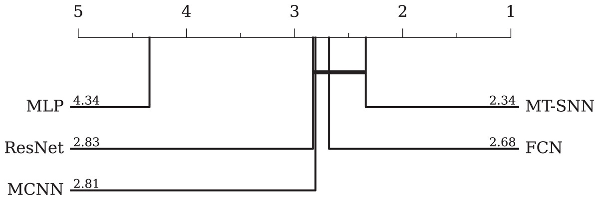
Figure 9: The critical difference diagram between MT-SNN and traditional DL methods.
Comparison with TSC-SNN work
The proposed MT-SNN is compared with previous TSC-SNN work on 24 univariate datasets from the UCR Time Series Classification Archive. The results are presented in Table 6, which shows the comparative performance of the proposed MT-SNN model against other state-of-the-art TSC-SNN models across various datasets. The MT-SNN model surpasses other models in the majority of datasets, achieving the highest accuracy in 19 out of 24 datasets.
| Dataset | GTE (Dey et al., 2022) | LSNN (Gaurav, Stewart & Yi, 2023) | CSNN (Gautam & Singh, 2020) | MT-SNN (Ours) |
|---|---|---|---|---|
| Beef | – | – | 86.66% | 87.50% |
| CBF | – | – | 100.00% | 100.00% |
| CinCECGTorso | – | – | 99.75% | 95.96% |
| Coffee | – | – | 100.00% | 100.00% |
| DiatomSizeR | – | – | 98.11% | 98.68% |
| Earthquakes | 71.94% | 80.43% | – | 81.25% |
| ECG200 | – | – | 92.00% | 93.75% |
| ECG5000 | – | 98.49% | – | 94.73% |
| FaceAll | – | – | 75.38% | 82.57% |
| FaceFour | – | – | 96.59% | 100.00% |
| FacesUCR | – | – | 85.36% | 93.45% |
| FordA | 80.37% | 93.56% | – | 94.62% |
| FordB | 64.32% | 82.72% | – | 85.50% |
| Gunpoint | – | – | 100.00% | 100.00% |
| ItalyPower | – | – | 97.37% | 97.36% |
| Lightning2 | – | – | 80.33% | 90.62% |
| Lightning7 | – | – | 83.56% | 90.62% |
| StarLightCurves | – | – | 97.91% | 97.79% |
| SyntheticControl | – | – | 100.00% | 100.00% |
| Trace | – | – | 100.00% | 100.00% |
| TwoPatterns | – | – | 100.00% | 100.00% |
| UWaveX | – | – | 80.37% | 80.43% |
| UWaveY | – | – | 76.68% | 72.80% |
| Wafer | 98.85% | 99.51% | 100.00% | 100.00% |
Comparison with CSNN: The MT-SNN achieves significant improvements on several datasets. For example, MT-SNN shows remarkable advancements in the FacesUCR and Lightning2 datasets, with accuracies of 93.45% and 90.62%, compared to CSNN’s 85.36% and 80.33%, respectively. While CSNN reaches 100% accuracy on seven datasets, MT-SNN additionally achieves 100% on the FaceFour dataset. Despite CSNN achieving better results on datasets such as CinTorso and uWaveY, the advantage is insignificant. It is also worth noting that CSNN contains only a single layer of spiking neurons and still uses ReLU as activation functions, whereas MT-SNN replaces all ReLU with spiking neurons in feature extraction, encoding along with decoding, demonstrating superior spiking plausibility.
Comparison with GTE and LSNN: GTE and LSNN were exclusively tested on vibration time series datasets. Within these datasets, MT-SNN demonstrated significant advantages. The sole exception was the ECG5000 dataset, where LSNN achieved a higher accuracy compared to MT-SNN; however, the difference was not substantial. Overall, MT-SNN exhibited more comprehensive and outstanding performance compared to both GTE and LSNN.
In summary, the results demonstrate the consistent performance of MT-SNN across multiple datasets, highlighting its generalizability and effectiveness. Remarkably, MT-SNN achieves these results without relying on specialized encoding schemes or pre-feature engineering techniques, using a very low timestep of 5 or 3. This underscores the inherent capability of SNNs to capture discriminative features directly from original time series data.
Visualization of spike encoder
To visualize the original one-dimensional data, the Lighting2 dataset is selected. The spike sequences of the feature maps extracted by the encoder in five time steps are plotted. For ease of visualization, the encoding of the first five channels is displayed, illustrating encoding effects at different timesteps as shown in Figs. 10, 11, 12.
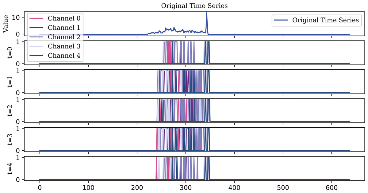
Figure 10: Due to its decay property, the LIF encoder fires spikes that are more dispersed over time compared to the IF and TAIF encoders.
However, this sparse representation compromises temporal precision by missing the rise in the original time series at the length of 400.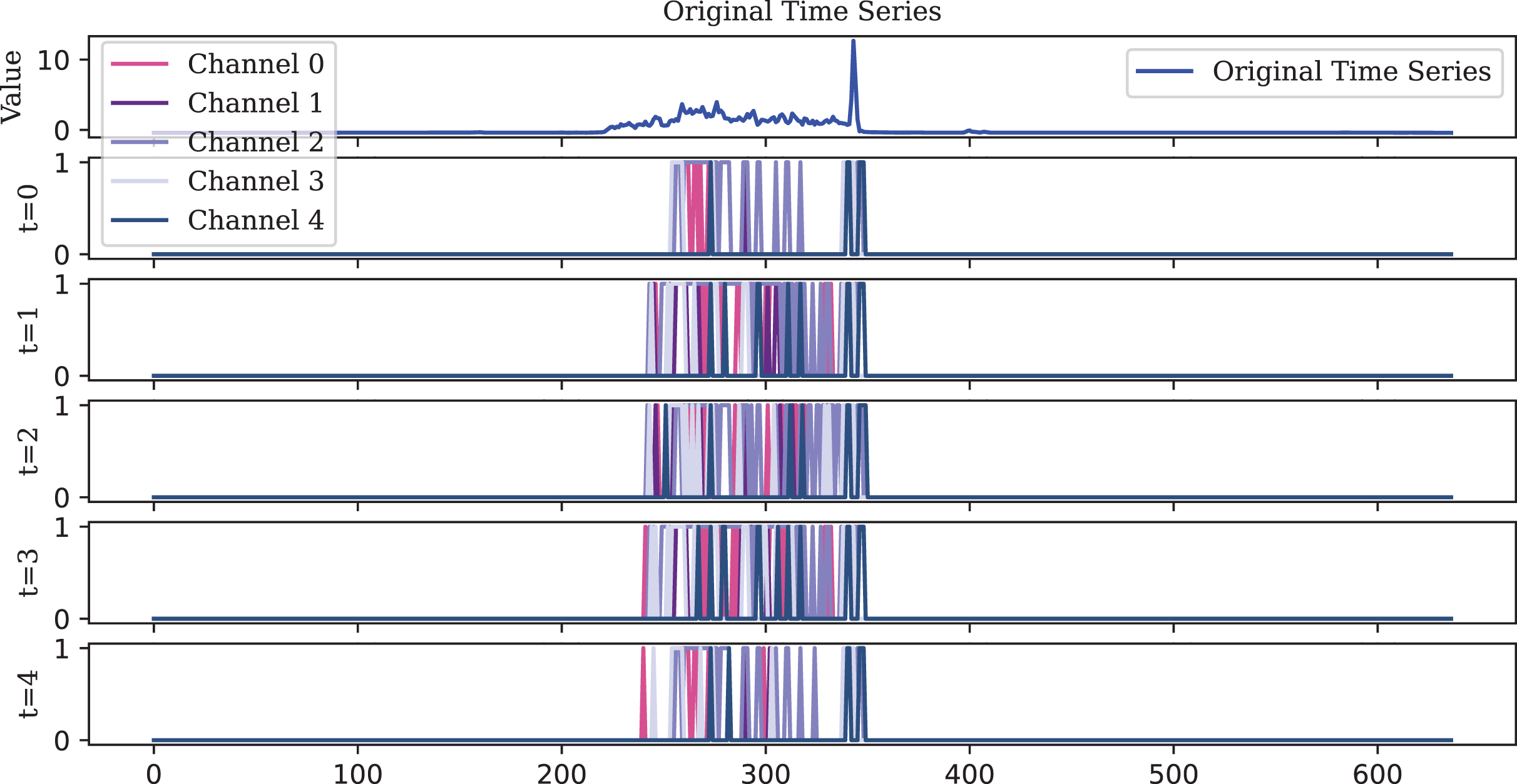
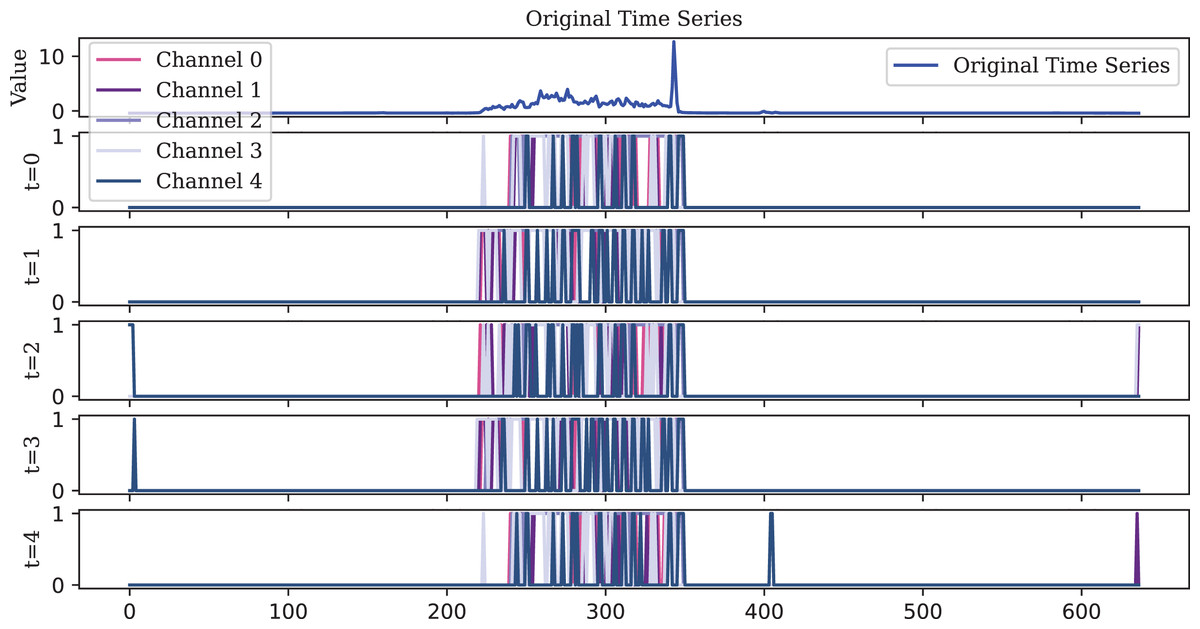
Figure 11: The IF encoder, functioning as an ideal integrator, generates a higher density spike representation.
However, this also results in lower robustness. In the final stage (t = 4), an abnormal spike, which should not have been fired, appeared at the end of the sequence.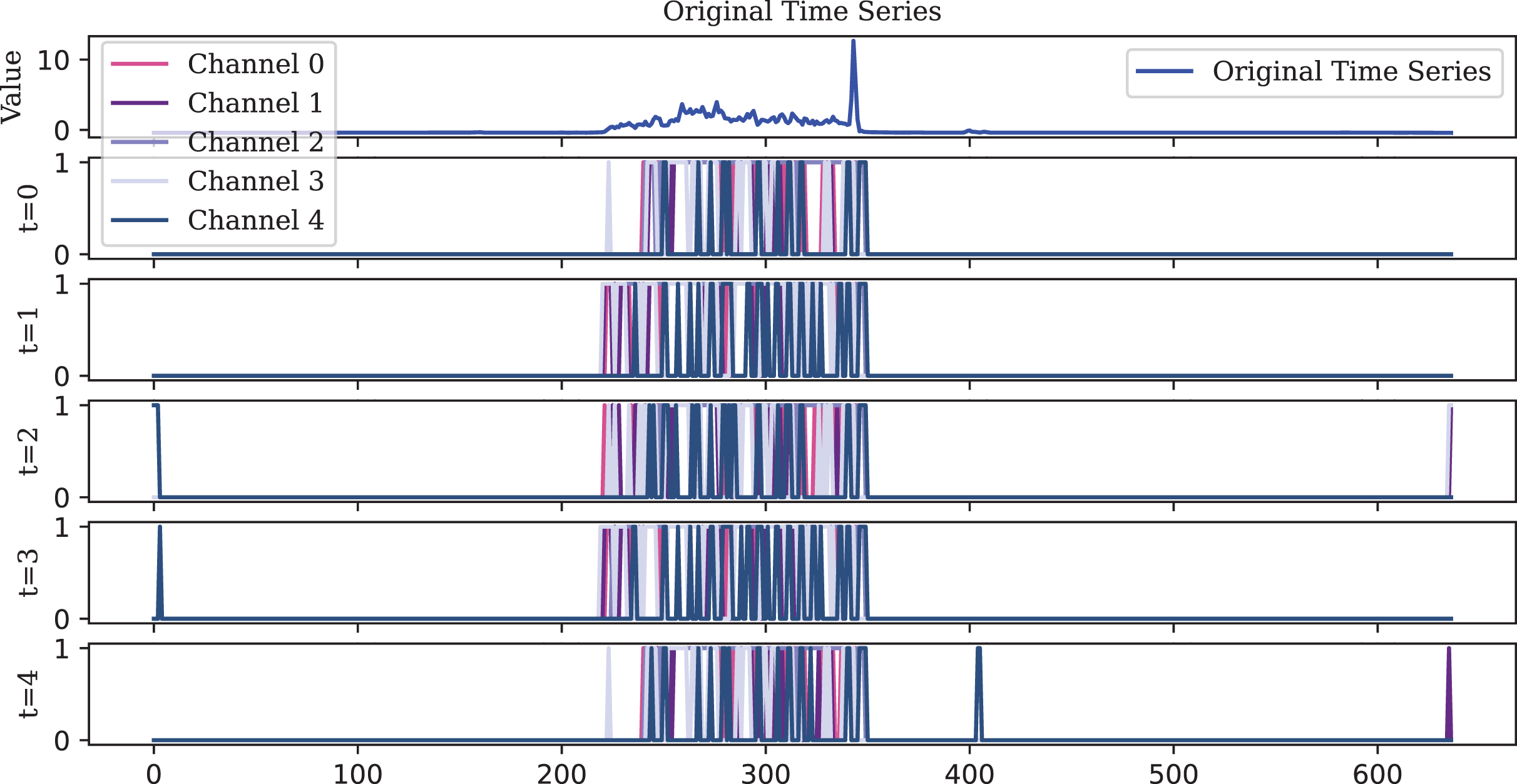
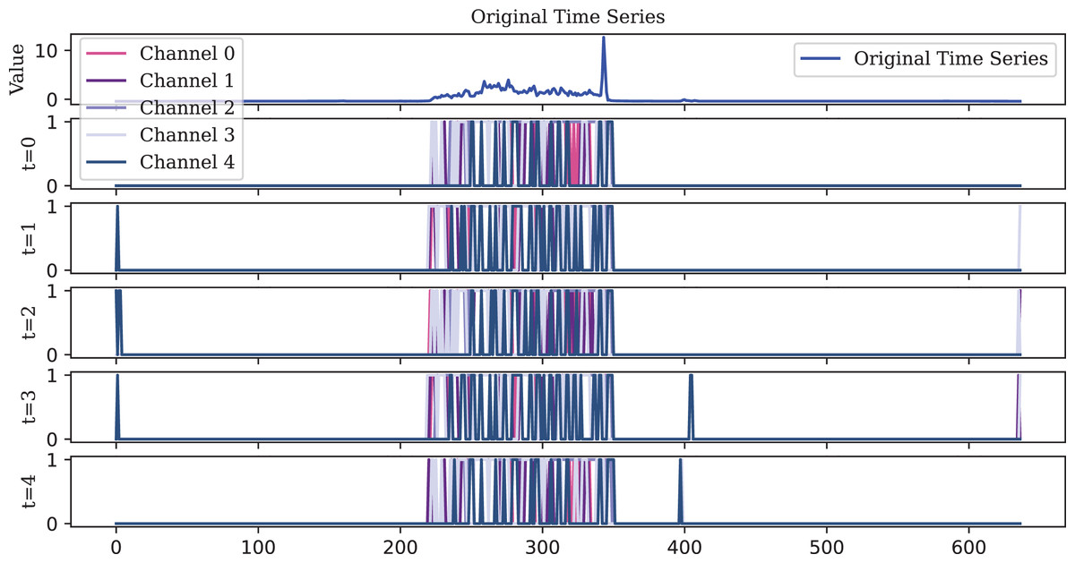
Figure 12: The TAIF encoder is similar to the IF encoder, but its spikes are more evenly distributed over time and more compact than those of the LIF encoder.
Due to its temporal adaptive feature, the TAIF encoder effectively captures the rise without producing abnormal spikes.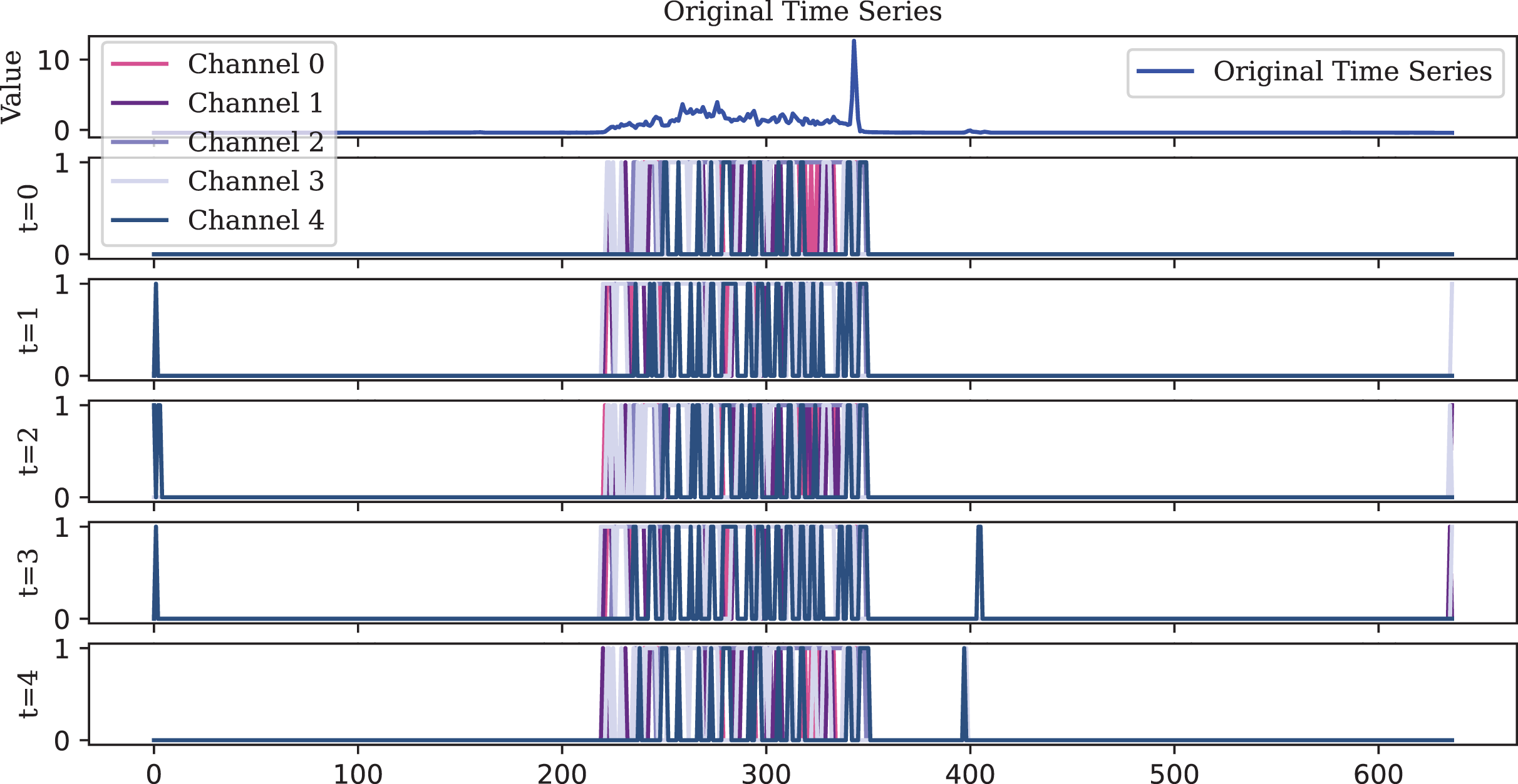
Observations illustrate that, in the early timesteps, the features extracted by the spike encoder are relatively sparse. However, as the timesteps progress, more features are activated, indicating that the TAIF encoder is capable of gradually extracting and accumulating key information from the input signals over time, forming an efficient spike encoding representation. This approach avoids the non-firing issue of the LIF encoder and the misfiring issue of the IF encoder.
In addition, Fig. 13 illustrates the comparison between IF and TAIF encoders in a single channel. Through a visual analysis of feature mappings across different timesteps and neurons, the effectiveness of the TAIF spike encoder in encoding time series data becomes evident. The overlay results demonstrate the overall encoding performance, while the feature mappings of individual channels reveal fine-grained encoding characteristics. This section includes the raw data, feature mappings at various timesteps, feature mappings of individual neurons, providing a comprehensive evaluation of the encoding performance of different spike encoders.
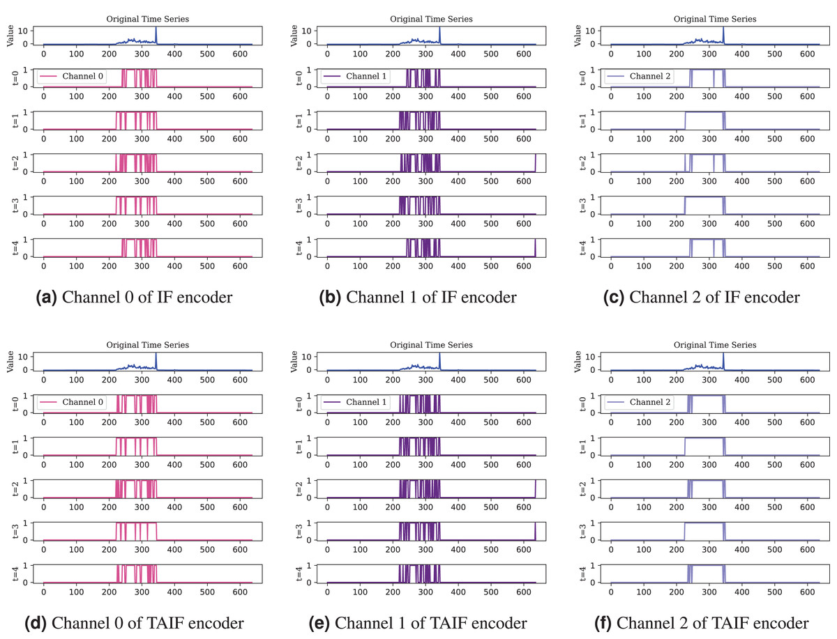
Figure 13: Comprasion of IF and TAIF encoder in single channel.
The TAIF encoder provides smoother encoding compared to the IF encoder, especially noticeable in less sensitive channel, maintaining a consistent and adaptive spiking pattern.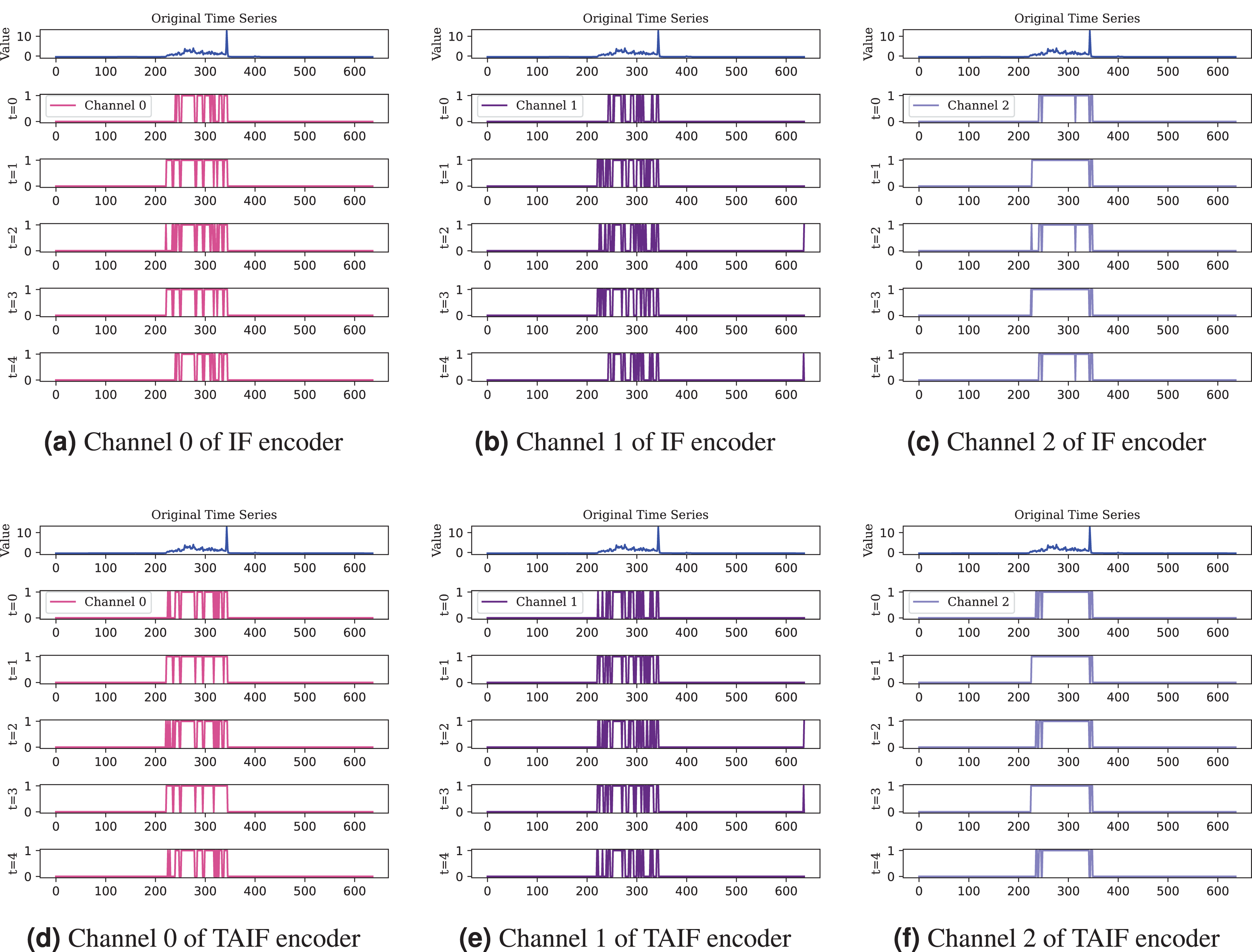
Noise tolerance in masked timesteps
In this section, we conduct an experiment to evaluate robustness under varying levels of Gaussian noise. By introducing Gaussian noise with different standard deviations to the original time series data, we aim to analyze the impact on the performance of IF and TAIF under Masked Timestep.
The datasets used for this analysis include the CBF, Coffee and Gunpoint datasets, each subjected to three different levels of Gaussian noise: 0.5, 1.0, and 1.5.
The performance metrics for each model under different noise conditions are summarized in Fig. 14.
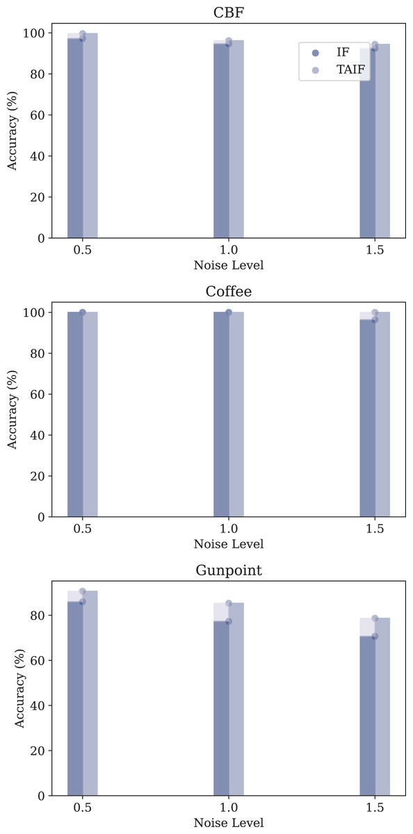
Figure 14: Evaluation of three datasets of noise tolerance of IF and TAIF in MT-SNN.
In the MT-SNN architecture, both models exhibit varying degrees of robustness to different levels of Gaussian noise. In the CBF and Coffee datasets, both models have a certain robustness, maintaining high accuracy across all noise levels. However, in the Gunpoint dataset, the TAIF model consistently outperforms the IF model across all noise levels. This dataset contains short sequences with localized temporal patterns, making it highly sensitive to noise. By introducing temporal adaptivity, TAIF achieves a more stable response to critical timesteps and thus preserves discriminative features more effectively, leading to greater robustness under Gaussian noise.
Training with restricted data subset
In this section, to simulate edge scenarios with limited device or training resources, real-time requirements, and costly annotation, the performance of the MT-SNN is evaluated on a restricted data subset. Unsolved binary classification tasks, which better reflect real-world situations, are selected. Their training sets are reduced to 10% of their original size, ensuring that each class has at least one sample, while the test sets remain unchanged.
To provide a thorough comparison, we also present the performance of Spiking Reservoir method using Gaussian Temporal Encoding (GTE) as described in Dey et al. (2022). Importantly, this method is trained on 20% of the training data. This comparison allows us to assess the relative performance and robustness of the MT-SNN under harsher constraints. The detailed settings and performance comparisons are provided in Tables 7 and 8.
| Datasets | Samples | GTE (20%) | MT-SNN (10%) |
|---|---|---|---|
| Earthquakes | 322 | 64 | 32 |
| ECG200 | 100 | – | 10 |
| ECGFiveDays | 23 | – | 2 |
| FordA | 3,601 | 720 | 360 |
| FordB | 3,636 | 727 | 362 |
| ItalyPower | 67 | – | 6 |
| Lightning2 | 60 | – | 6 |
| MoteStrain | 20 | – | 2 |
| SonyAIBO | 20 | – | 2 |
| SonyAIBOII | 27 | – | 2 |
| Yoga | 300 | – | 30 |
| Datasets | GTE | MT-SNN (10%) | MT-SNN (100%) |
|---|---|---|---|
| Earthquakes | 63.64% | 80.47% | 81.25% |
| ECG200 | – | 85.42% | 93.75% |
| ECGFiveDays | – | 70.74% | 93.35% |
| FordA | 74.27% | 92.54% | 94.62% |
| FordB | 59.57% | 78.12% | 85.50% |
| ItalyPower | – | 86.80% | 97.74% |
| Lightning2 | – | 78.33% | 90.62% |
| MoteStrain | – | 89.42% | 92.27% |
| SonyAIBO | – | 67.71% | 98.17% |
| SonyAIBOII | – | 79.31% | 91.70% |
| Yoga | – | 60.99% | 85.50% |
The adaptability of the MT-SNN using direct encoding enables it to perform significantly better than the GTE using temporal encoding, even with only half the amount of training data. Despite the reduced size of the training set, the MT-SNN reaches reasonably high accuracy on several datasets with limited training samples. For datasets with a large number of original training samples, such as Earthquake, FordA and FordB, the performance of MT-SNN in a restricted setting is almost comparable to that of the full dataset, outperforming GTE under more challenging conditions. Additionally, for datasets with only a few training samples, MT-SNN still achieves acceptable performance, even reaching levels comparable to those with the full dataset in cases like MoteStrain and Lightning2. The lower results in Yoga and SonyAIBO are probably due to the inadequate representation in the 10% training data for the spike encoder. However, considering the reduction in sample size, this decrease is acceptable. In conclusion, the enhanced performance of MT-SNN under more constrained conditions highlights its robustness and adaptability compared to the Spiking Reservoir method.
Conclusion
In this article, we propose the MT-SNN architecture to address the issue of temporal redundancy in TSC-SNN when training from scratch. As a purely end-to-end model, MT-SNN employs a simple and effective direct encoding method, eliminating the need for pre-trained encoders and data augmentation while achieving SoTA performance in univariate TSC tasks with stronger generalization capabilities. The masked timestep method improves efficiency and reduces computational cost by selectively masking less informative timesteps, thereby focusing computational resources on the most significant features. Furthermore, the introduction of TAIF neurons provides MT-SNN with greater noise tolerance, allowing it to maintain robust performance even in the presence of exsiting noisy input data.
Compared to RC methods, MT-SNN demonstrates enhanced learning capabilities with smaller datasets, making it particularly suitable for edge scenarios where computational resources and data availability are limited. The architecture design inherently supports efficient implementation on edge devices, offering significant advantages in low-latency and real-time processing environments. In future work, we plan to deploy MT-SNN on specialized hardware, such as neuromorphic chips, to fully leverage its computational efficiency and low power consumption.
Further, we aim to refine the encoding method to further enhance the performance and adaptability of the models. We will also extend the application of the masked timestep method to multivariate TSC tasks, thereby broadening the scope and utility of MT-SNN across diverse real-world applications. At present, the evaluation is limited to benchmark univariate datasets, and its effectiveness in multivariate and real-world noisy environments remains to be validated. Moreover, we intend to optimize the MT method to enable automatic adjustment of the reduction of timesteps, replacing the current reliance on manual settings. This optimization will involve developing adaptive algorithms that can dynamically determine the most appropriate timestep reduction strategy based on the property of the input data.