
Deriving groundwater storage anomalies based on GRACE data and drought prediction using deep learning
- Published
- Accepted
- Received
- Academic Editor
- Giovanni Angiulli
- Subject Areas
- Algorithms and Analysis of Algorithms, Scientific Computing and Simulation, Neural Networks
- Keywords
- GRACE data, Standardized groundwater index, Deep learning models, Shaanxi Province
- Copyright
- © 2026 Tian et al.
- Licence
- This is an open access article distributed under the terms of the Creative Commons Attribution License, which permits using, remixing, and building upon the work non-commercially, as long as it is properly attributed. For attribution, the original author(s), title, publication source (PeerJ Computer Science) and either DOI or URL of the article must be cited.
- Cite this article
- 2026. Deriving groundwater storage anomalies based on GRACE data and drought prediction using deep learning. PeerJ Computer Science 12:e3459 https://doi.org/10.7717/peerj-cs.3459
Abstract
The sustainability of water resources is significantly threatened by groundwater drought, primarily due to the increasing impacts of climate change. Therefore, understanding the variability of water resources and making accurate projections regarding their future availability is crucial. This study focuses on Shaanxi Province, which is divided into three distinct regions: Guanzhong in the center, Southern Shaanxi, and Northern Shaanxi. Each region has vastly different climates, which complicates drought monitoring. This study utilized data from the Global Land Data Assimilation System (GLDAS) and the Gravity Recovery and Climate Experiment (GRACE) satellites to analyze the changes in groundwater storage anomalies (GWSA) in Shaanxi Province from 2002 to 2021. We developed the Standardized Groundwater Index (SGI) to elucidate the spatial and temporal characteristics of groundwater drought and its changing trends. The Mann-Kendall (MK) trend test was employed to quantitatively assess groundwater drought conditions in three regions. Furthermore, to enhance drought monitoring and prevention capabilities, we applied four deep learning models: long short-term memory (LSTM), convolutional neural network–long short-term memory (CNN-LSTM), bidirectional long short-term memory (BiLSTM), and long short-term memory with attention mechanism (LSTM-Attention) to predict drought indices. Our findings indicate that while the drought trend in Southern Shaanxi is not as prominent, it is declining in Northern Shaanxi and Guanzhong. Overall, the average accuracy of the deep learning models in forecasting drought indices across all grid points in the three regions is above 84%, with the CNN-LSTM model demonstrating the best performance. This research highlights the significant potential of deep learning approaches for drought monitoring and forecasting, providing a new and effective strategy for water resource management and early warning systems. The implications for drought monitoring and prevention in Shaanxi Province and beyond are substantial, as these methods can enhance responses to drought occurrences and ensure the sustainable use of water resources.
Introduction
Drought impacts escalate from local to global scales. In Shaanxi Province, located in the water-stressed northwest of China, 22 large-scale meteorological drought events were recorded during 1961–2024; events after 2000 exhibited significantly longer durations and expanded spatial coverage (Wang et al., 2025). In 2023 the province’s per-capita water resources were only 50% of the national average (ranking 24th nationwide), while groundwater abstraction reached 2.73 billion m3 (ranking 9th nationally), underscoring a heavy reliance on aquifers (Ministry of Water Resources of the People’s Republic of China, 2024). Globally, 30% of the terrestrial surface experienced moderate-to-severe drought in 2022, and the global drought area has expanded at a rate of 0.36% yr−1 since 1981 (Gebrechorkos et al., 2025). These facts highlight the urgent need for robust, high-resolution groundwater-drought monitoring and prediction tools in Shaanxi and similar semi-arid regions worldwide.
Groundwater drought (Di Nunno & Granata, 2024; Gumus, 2023) is a critical natural resource issue that poses a significant danger to global agricultural productivity and socioeconomic activity (Deng et al., 2024). Monitoring and preventing drought has become increasingly important, especially given the combined effects of climate change and human activities (Acreman, Casier & Salathe, 2022). Shaanxi, a key province in China, is characterized by its unique geographic location, diverse climate, and significant regional variations in groundwater resources. These factors, combined with low rainfall and rising water demand, complicate drought monitoring in the area. Numerous scholars, both domestic and international, have undertaken extensive research on drought indices. McKee, Doesken & Kleist (1993) established the Standardized Precipitation Index (Karbasi et al., 2024) (SPI) after analyzing the drought in Colorado in the United States, and discovering that precipitation followed a skewed distribution. The Palmer Drought Severity Indicator (PDSI), created by American meteorologist Wayne Palmer in 1965, is another widely used drought index in meteorology, climate studies, agriculture, and hydrological water resources management. The Standardized Precipitation Evapotranspiration Index (SPEI) evaluates the relationship between precipitation and evapotranspiration, including plant transpiration. In addition, SPEI quantitatively describes an area’s level of aridity or wetness by standardizing time-series data on precipitation and evapotranspiration.
The integration of deep learning with groundwater drought research provides a novel alternative to conventional groundwater modeling and forecasting techniques, which are largely based on statistical and physical models. Traditional methods, including time series analysis, grey system models, analytical solutions, and distributed hydrological models, offer detailed insights into groundwater systems but are often limited in practical application. These limitations stem from high computational costs, the complexity of modeling physical processes, and the extensive hydrogeological data required for model calibration and validation (Clark, Pagendam & Ryan, 2022). In contrast, the integration of deep learning provides a more efficient, data-driven approach that effectively handles complex non-linear relationships and reduces dependency on extensive data, thereby enhancing the accuracy and efficiency of groundwater modeling and forecasting. Within this field, long short-term memory (LSTM) networks are frequently used to create prediction models of groundwater level fluctuations, as they are particularly adept at capturing temporal dependencies in data (Cai et al., 2021; Zhou et al., 2024). These models are ideally suited to represent the dynamic nature of groundwater systems (Ramakrishnan et al., 2024). However, the prediction of groundwater storage anomalies (GWSA) derived from Gravity Recovery and Climate Experiment (GRACE) data using the LSTM model has also revealed certain limitations, particularly the model’s vulnerability to overfitting. So, we explored whether other models developed based on the LSTM model could work better than the LSTM.
This study aims to analyze the groundwater drought conditions in Shaanxi Province from 2002 to 2021 and identify suitable deep learning models for predicting the Standardized Groundwater Index (SGI). To the best of our knowledge, this study is the first to integrate the Standardized Groundwater Index with deep-learning frameworks and to systematically compare the applicability and predictive accuracy of LSTM and its three derivative architectures for groundwater-drought forecasting. To achieve this objective, data from the GRACE satellite and the Global Land Data Assimilation System (GLDAS) were utilized to derive and analyze the GWSA over the study period. Specifically, Shaanxi Province was divided into 576 study areas based on a regular grid with a spatial resolution of 0.25° in both latitude and longitude. To model GWSA data collected from these study areas, five distinct distribution functions were evaluated: Pearson III, Beta, Gumbel, Normal, and Extreme Value distributions. To model the GWSA effectively, the Pearson Type III distribution was identified as the most suitable function and subsequently used to construct the SGI. The Mann-Kendall (MK) trend test was applied to the SGI (Guo et al., 2021) values of all grid points, enabling a quantitative assessment of groundwater drought conditions across different regions of Shaanxi Province. Additionally, four advanced deep learning models (Alabdulkreem et al., 2023; Aybey & Gümüş, 2023) were explored to enhance the accuracy and effectiveness of drought index prediction (Chen et al., 2023) and to improve drought monitoring and prevention capabilities. These models included LSTM, convolutional neural network–long short-term memory (CNN-LSTM), bidirectional long short-term memory (BiLSTM), and long short-term memory with attention mechanism (LSTM-Attention). The application of these models in groundwater sustainability research (Secci et al., 2021) holds significant practical implications. It not only provides valuable reference experience for drought studies in Shaanxi Province and other regions with complex geographic and climatic conditions but also enables more accurate prediction and monitoring of changes in groundwater resources. This approach ultimately offers a robust scientific basis for groundwater sustainability management.
Study area and data
Study area
Shaanxi Province, located in the central part of China, extends along the middle reaches of the Yellow River. The province’s geographic coordinates range from 105°29′ to 111°15′ east longitude and from 31°42′ to 39°35′ north latitude. Shaanxi is notable for its diverse natural geography, which comprises three distinct regions: Northern Shaanxi, Guanzhong, and Southern Shaanxi. Northern Shaanxi, lying at the center of the Loess Plateau (Di Nunno & Granata, 2024), features plateaus and hills with long gullies and ravines. This region has low vegetation coverage and an ecologically fragile environment, typical of the arid climate of the Loess Plateau, which receives limited precipitation. The Guanzhong region in central Shaanxi contains one of the most extensive plains in northwestern China. It enjoys a mild climate with four distinct seasons, flat terrain, and fertile soil, making it a hub for developed agriculture, often called “800 miles of Qinchuan.” In contrast, Southern Shaanxi, situated south of the Qinling Mountains, is predominantly mountainous terrain and experiences a humid climate characteristic of the subtropical zone (Gautam, Chandra & Henry, 2024). This region is rich in water resources, with the Han River and other rivers flowing through it, and it boasts high forest coverage (Fig. 1).
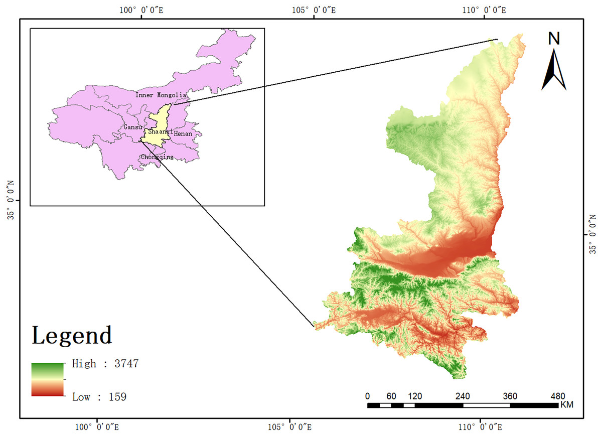
Figure 1: Topographic map of Shaanxi Province with digital elevation model (DEM).
Data
GRACE satellite data are utilized to capture monthly measurements of the Earth’s gravity field by monitoring changes through gravimetric satellites (Xu et al., 2023; Castle et al., 2014). These changes are then translated into a representation of total terrestrial water storage changes expressed as equivalent water column height. The GRACE data used in this study are from the Center for Space Research (CSR) (https://www2.csr.utexas.edu/grace/) in Austin, Texas, USA. Specifically, the CSR GRACE Mascon data were used, which provide information on terrestrial water storage anomalies (TWSA). These data have been oversampled from their native resolution of 3° to a spatial resolution of 0.25° × 0.25°. The temporal resolution of the dataset is one month. The TWSA anomalies have been adjusted for surface mass bias, with the baseline established using the average data from January 2004 to December 2009.
The GLDAS (https://hydro1.gesdisc.eosdis.nasa.gov/data/GLDAS) assimilation system data integrates ground observation and satellite remote sensing data to inform the land surface model. In this study, month-by-month shallow surface water storage data from the Noah land surface model (GLDAS_NOAH025_M.2.1) within the GLDAS framework. The data covers the time period from April 2002 to April 2021 and includes data for soil water storage, snow water equivalent, and canopy water storages at depts of 0–10 cm, 10–40 cm, 40–100 cm, and 100–200 cm, all with a spatial resolution of 0.25° × 0.25°. To ensure consistency in the GRACE data (Sade et al., 2014), we applied the same baseline from January 2004 to December 2009 and calculated month-by-month changes in shallow surface water storage by comparing the month-by-month data with the baseline value. The GLDAS data contained rainfall, snow water equivalent, and soil moisture. This study focuses on the changes in soil water content, especially in soil moisture and snow water equivalent at various depths. Given the specific geographic characteristics of Shaanxi Province, we chose these variables for our analysis.
In this study, the data from GRACE and GLDAS span from April 2002 to April 2021. The subsequent analysis leveraged spatial grid points with a resolution of 0.25° × 0.25°, encompassing the broad global area covered by the GRACE satellite.
Methods
Calculating groundwater storage anomalies
The total terrestrial water storage includes groundwater, surface water, canopy water, and snow water. Canopy water is negligible in arid and semi-arid regions (Felfelani et al., 2017; Lv et al., 2019), so the calculation of groundwater storage anomaly can be performed using the following equation:
(1) where GWSA represents the change in groundwater storage (in mm), TWSA represents the change in terrestrial water storage, SMSA represents the change in soil water storage, SWESA represents the change in snow water equivalent, and CSWA represents the change in canopy water storage. Due to technical issues such as satellite sensing problems (including instrument malfunctions, data gaps during calibration, environmental interference, battery management issues, and signal noise), some data are missing from the GRACE dataset. To address this challenge, the missing data are interpolated using the mean value interpolation method, which involves using the average values of adjacent months to fill in the missing data. Soil moisture data are particularly important because they directly reflect the water status in the soil, which is closely related to canopy water storage. Since soil moisture can be absorbed by plant roots and stored in the canopy, we have decided not to consider the canopy water factor in this study.
Standard Groundwater Drought Index (SGI)
To calculate the Standardized Groundwater Drought Index (SGI), an optimal probability density function (PDF) is first selected to fit the groundwater storage data and obtain the corresponding fitting parameters. The cumulative distribution function (CDF) is then derived by integrating the chosen PDF. Finally, the CDF values are converted into SGI values using the inverse function of the standard normal distribution.
Firstly, selecting an appropriate probability density function (PDF) to accurately fit the groundwater storage data is crucial. To evaluate whether the data conform to a specific distribution, we employ the Anderson-Darling (AD) test. This test involves calculating a test statistic and comparing it with critical values to determine if the data significantly deviate from the hypothesized distribution. Below is the procedure for calculating the AD test:
(2)
(3)
(4) where n is the number of samples; i is the rank order of the data (all data are to be arranged from smallest to most significant); and F(x) is the normal distribution cumulative probability density function. We calculated the AD-adjusted value based on these parameters, denoted as AD*. Subsequently, we determined the P-value based on the AD* value. If the P-value is less than 0.05, this indicates that the data are statistically significantly out of line with the distribution of that density function; conversely, if the P-value is greater than or equal to 0.05, the data are in line with the distribution of that density function.
After passing the AD test and identifying a suitable probability density function (PDF), one can proceed to calculate the SGI index. This process involves fitting the data to the chosen PDF to determine the parameters of the fitted distribution. Once these parameters are established, they are used to calculate the corresponding cumulative distribution function (CDF) values. Finally, we apply the inverse function of the CDF of the standard normal distribution, which has a mean of zero and a standard deviation of 1, to convert the CDF values into SGI values.
The SGI is calculated as follows
(5) where fit is the fitting function, θ is the parameter that receives the fit, f(Xk) is the chosen probability density function, and Xk is the groundwater level data for the kth grid point.
(6)
Further, f(t, θ) is the same PDF as in Eq. (6), and F(x,θ) is a CDF.
(7) where Φ-1 is the inverse function of the cumulative distribution function of the standard normal distribution.
The SGI (Akl & Thomas, 2024) was developed based on the Standardized Precipitation Index (SPI) to measure changes in groundwater storage (Zeng et al., 2024). An SGI greater than 0 indicates groundwater levels above the average during the baseline period (Dubois & Larocque, 2024), suggesting wet conditions; conversely, an SGI less than 0 indicates levels below the average, potentially signifying drought conditions. An SGI equal to 0 indicates groundwater levels at the average during the baseline period. In this study, we evaluated five standard probability density functions—Pearson Type III, Beta, Gumbel, normal, and gamma distributions—to determine which best describes groundwater level changes. Through comparative analyses, we selected the most appropriate model for our data.
The Mann-Kendall (MK) trend test
The MK trend test is a well-established non-parametric statistical method for analyzing trends in time series data (Ren et al., 2024). The core principle of the MK test involves comparing each pair of data points in a time series to assess whether the overall time series shows a trend change. This is done by evaluating the correlation between the data points. One of the advantages of the MK test is that it does not require any specific assumptions about the distribution of the data, making it particularly suitable for trend analysis in hydrology and can effectively test the statistical significance of trends observed in the data. We begin by assuming a set of time series for analysis.
(8)
(n is the number of variables and n ≥ 10) to establish the standard normal distribution statistic Z.
(9)
The procedure for calculating the parameters in Eq:
(10)
(11)
(12) where Var(S) is the variance, S is the statistic of an approximately normal distribution, q denotes the number of groups with the same value in the data, and tp is the number of data with the same value as the pth group.
The starting point for the MK test is the null hypothesis H0, which assumes that the dataset is independently and identically distributed, i.e., no trend exists in the data. We set a significance level α and determine the critical value Z1 − α/2. If the absolute value of the test statistic Z |Z| exceeds this critical value, we have sufficient evidence to reject the null hypothesis H0 and thus conclude that the data series shows a statistically significant change in trend. Specifically, if the value of Z is greater than 0, it indicates a significant upward trend in the series. Conversely, if the value of Z is less than 0, it signifies a significant downward trend. If the absolute value of the test statistic Z does not exceed the critical value, we do not have sufficient evidence to reject the null hypothesis H0, which asserts that the data series does not exhibits a significant trend change.
Selection and validation of optimal functions for GWSA
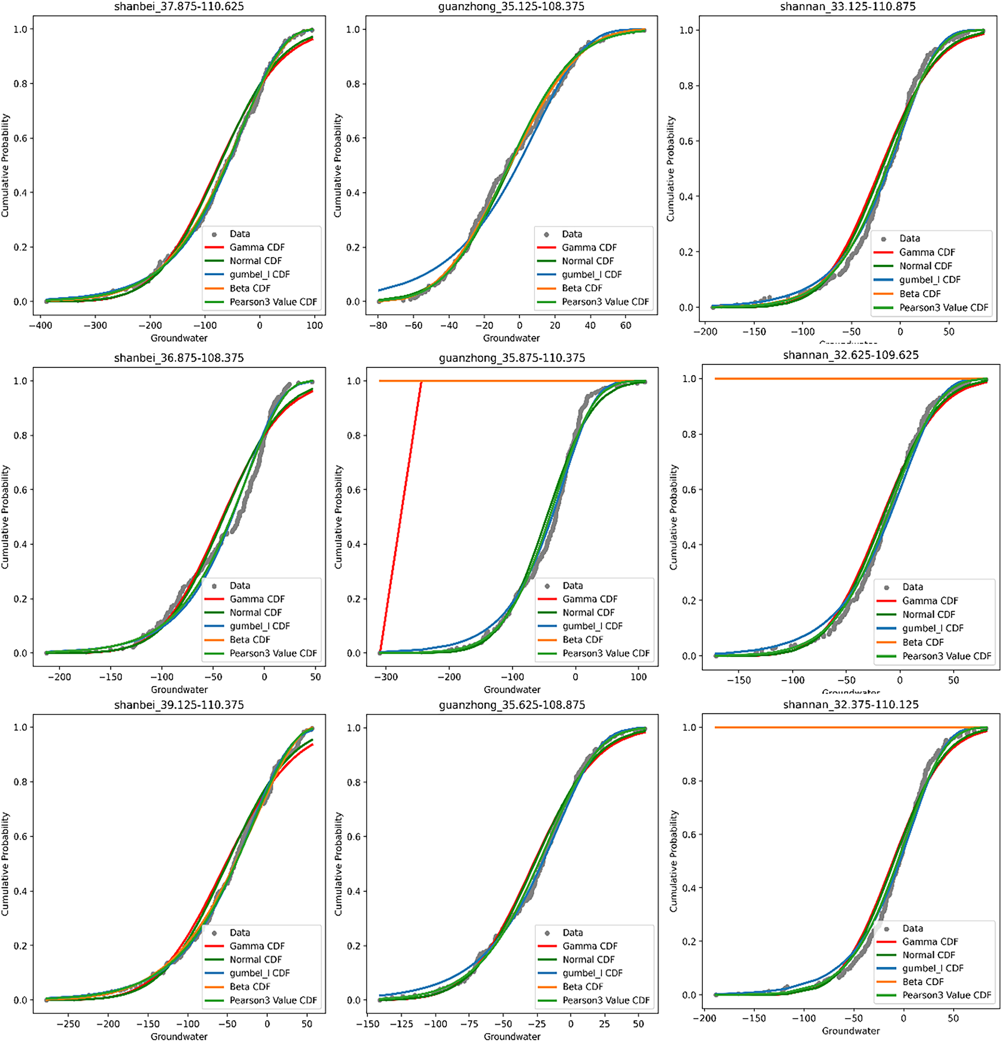
In this study, we randomly selected three grid points from three regions of Shaanxi Province: Northern Shaanxi, Southern Shaanxi, and Guanzhong. Our goal was to analyze the best-fit functions of GWSA data and their cumulative distribution function (CDF) curves for the grid points across these regions. Specifically, there are 256 grid points in Northern Shaanxi, 128 in Guanzhong, and 192 in Southern Shaanxi. In this study, three grid points were randomly selected from each region to ensure representation of the entire study area. This strategy was implemented to minimize selection bias and enhance the generalizability and reliability of the outcomes. The primary goal was to determine the distribution that most accurately characterizes the GWSA data.
The coordinates of the three randomly selected grid points for the Northern Shaanxi region were 37.875°N, 110.625°E; 36.875°N, 108.375°E; and 39.125°N, 110.375°E. Our analysis reviewed that the Pearson Type III and Beta distributions best fit the GWSA data for Northern Shaanxi. For the Guanzhong region, the coordinates of the three random grid points are 35.125°N, 108.375°E; 35.875°N, 110.375°E; and 35.625°N, 108.875°E. The fitting analysis showed that neither the Gamma nor the Beta distributions were well-suited for the region; the Pearson Type III distribution was determined to be the most appropriate. In Southern Shaanxi, the coordinates of the three grid points are 33.125°N, 110.875°E; 32.625°N, 109.625°E; and 32.375°N, 110.125°E. The Beta distribution was found to be the least suitable for this region.
To further corroborate the selection, the Anderson–Darling (AD) test was applied to all 576 grid points across Shaanxi Province. A cell was deemed to have passed the test if its p-value exceeded 0.5. The goodness-of-fit of the Pearson type III, Beta and Gumbel distributions was evaluated separately. The dataset included 256 points in Northern Shaanxi, 128 points in Guanzhong, and 192 points in Southern Shaanxi. Following this, we documented the number of grid points that successfully passed the AD test across these regions to further analyze the distributional characteristics of the GWSA data. This statistical outcome will offer valuable insights into data fitting across different regions, thereby enhancing our capability to more accurately understand and predict drought conditions in Shaanxi Province.
Deep learning models
This study examines the performance of four deep learning models designed to predict the Standardized Groundwater Index (SGI) across all grid points in Shaanxi Province. The models evaluated include the LSTM model, the CNN-LSTM model, the BiLSTM model, and the LSTM-Attention model. These models employ SGI values as input variables and generate SGI predictions as output variables. Given the limited number of data samples, the training and testing datasets were divided in a 9:1 ratio. To optimize the models’ ability to learn complex patterns within the data while maintaining computational efficiency, the mean squared error (MSE) was used as the loss function, and the Adam optimizer was used with a learning rate of 0.01.
-
(1)
LSTM model
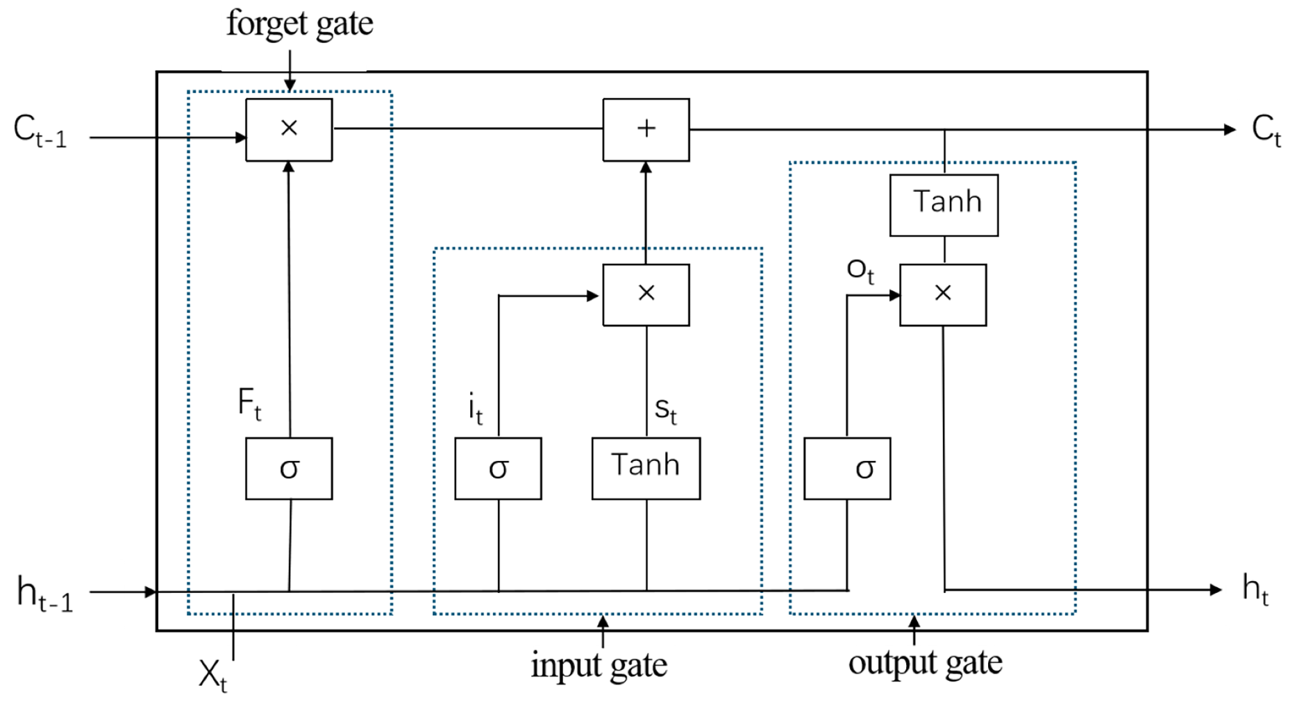
LSTM (Sadeghzadehyazdi, Batabyal & Acton, 2021) is a specialized form of Recurrent Neural Network (RNN) designed to effectively handle long-term dependencies within sequential data. Central to LSTM’s functionality is its unique cell structure, which comprises three primary gates: the forget gate, the input gate, and the output gate. These gates regulate the flow of information within the cell, thereby enabling the capture of long-term dependencies. The forget gate determines which information to discard from the cell state, the input gate decides which new information to store, and the output gate controls which part of the cell state is outputted. This intricate gating mechanism allows LSTM to dynamically manage its internal state, making it highly effective for tasks involving long sequences. The architectural of the LSTM model (Fig. 2).
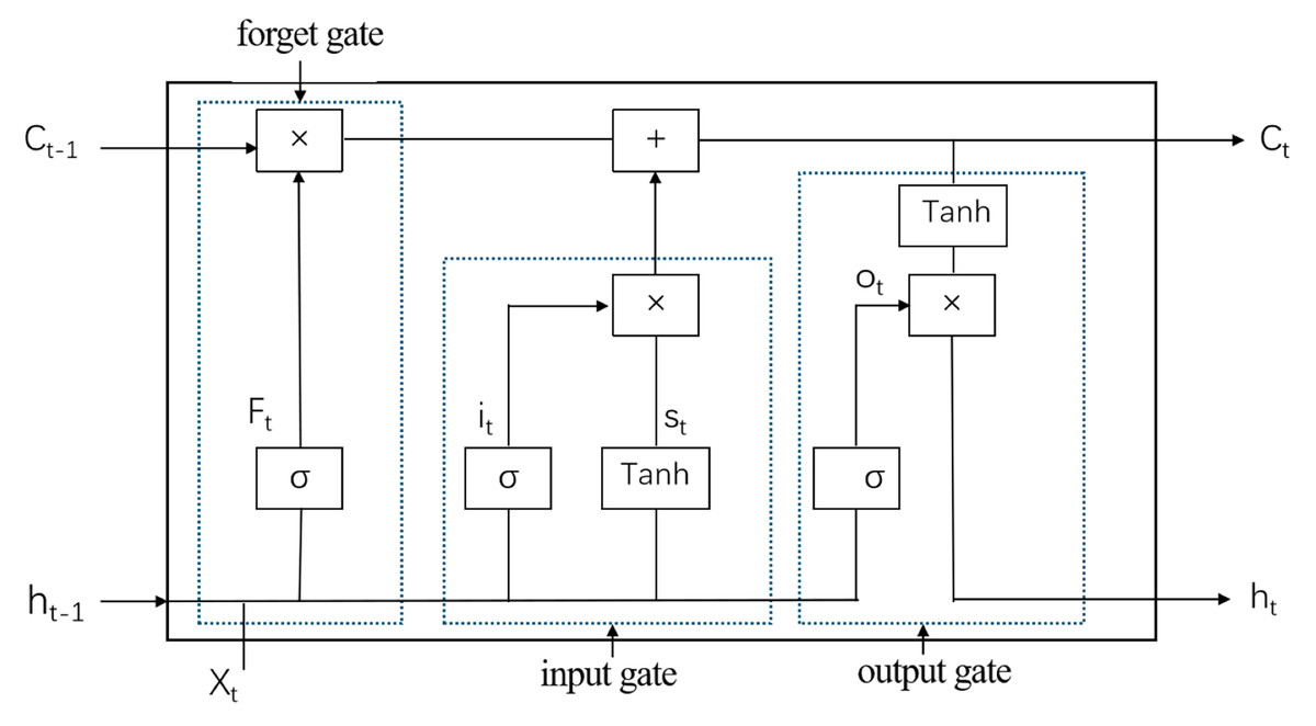
Figure 2: LSTM model diagram.
The mathematical formulation of LSTM is presented as follows:
(13)
(14)
(15)
(16)
(17)
(18) where * denotes element-by-element multiplication, ht is the hidden state at the current time step, xt is the input, and W and b are the weights and biases, respectively. Here ft, it, ot are the activation values of the forgetting gate, the input gate and the output gate respectively, st is the candidate input cell and σ is the sigmoid activation function.
In this study, the proposed model architecture comprises a single LSTM layer designed to process sequential data effectively. The LSTM layer has an input dimension of 4 and a hidden layer dimension of 4, with 2 layers in total. This configuration enables the LSTM to capture both short-term and long-term dependencies within the data. Subsequently, the output from the LSTM layer is connected to a fully connected layer with an output dimension of 1, which generates the final predictions.
-
(2)
CNN-LSTM model
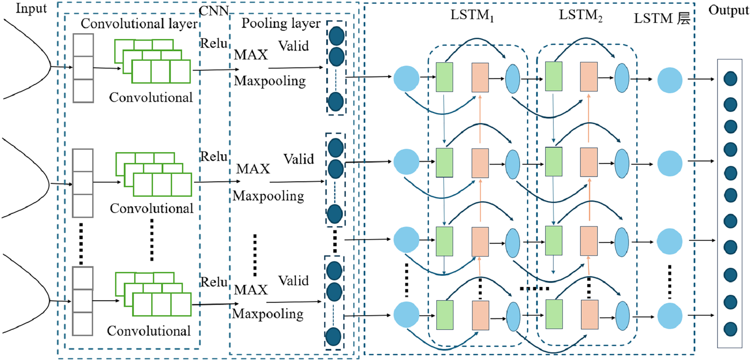
The CNN-LSTM model (Cui et al., 2024; Bi et al., 2024) represents a hybrid architecture that merges the feature extraction capabilities of CNNs with the sequential processing capabilities of LSTM networks. This integration enables the model to effectively manage spatiotemporal data by capturing both spatial and temporal dependencies. Specifically, the CNN component is tasked with extracting spatial features from the input data (Lessels & Bishop, 2020), which are subsequently fed into the LSTM component for temporal sequence processing. This dual-layered approach allows the model to identify complex patterns that may not be readily apparent when using CNNs or LSTMs in isolation. Conversely, traditional LSTM models concentrate exclusively on temporal dependencies and are unable to extract spatial features, rendering them less effective for data with significant spatial components. Thus, the CNN-LSTM model provides a more holistic methodology for analyzing data that exhibit both spatial and temporal characteristics. The architectural of the CNN-LSTM model (Fig. 3).
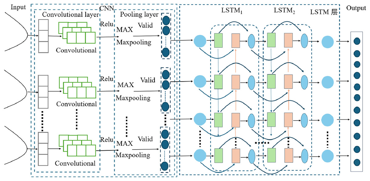
Figure 3: CNN-LSTM model diagram.
In this study, the proposed model architecture integrates a CNN layer with a LSTM layer to enhance the processing of sequential data. The CNN layer, designed with an input channel dimension of 4, utilizes a Conv1D operation with 12 output channels, a kernel size of 3, and padding of 1, followed by a ReLU activation function. This CNN layer effectively captures local patterns within the input sequences. Subsequently, the output from the CNN layer is fed into an LSTM layer with a hidden layer dimension of 4 and 2 layers, which is capable of capturing long-term dependencies in the data. Finally, the LSTM output is connected to a fully connected layer with an output dimension of 1, which generates the final predictions.
-
(3)
BiLSTM model
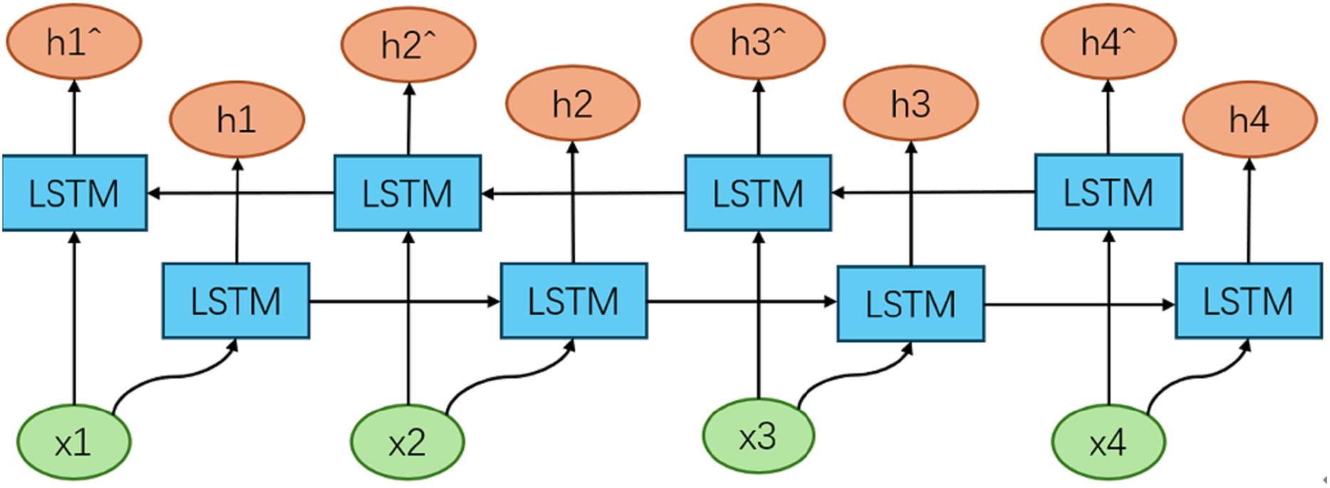
The BiLSTM model (Talebi, Torabi & Daneshpour, 2024) extends the traditional LSTM architecture by incorporating two independent LSTM layers that process the input sequence in both forward and backward directions. This dual-direction processing enables the model to capture both past and future context, thereby providing a more comprehensive representation of the sequence data. Specifically, the forward LSTM layer processes the sequence from the beginning to the end, capturing information from the past, while the backward LSTM layer processes the sequence from the end to the beginning, capturing information from the future. The outputs of these two layers are then combined, typically through concatenation or summation, to produce the final hidden states that encapsulate both forward and backward context. This bidirectional approach allows the BiLSTM model to outperform traditional LSTM models in tasks that require a deep understanding of context, such as natural language processing and time series prediction, where both preceding and subsequent information is crucial for accurate analysis and prediction. The architectural of the BiLSTM model (Fig. 4).
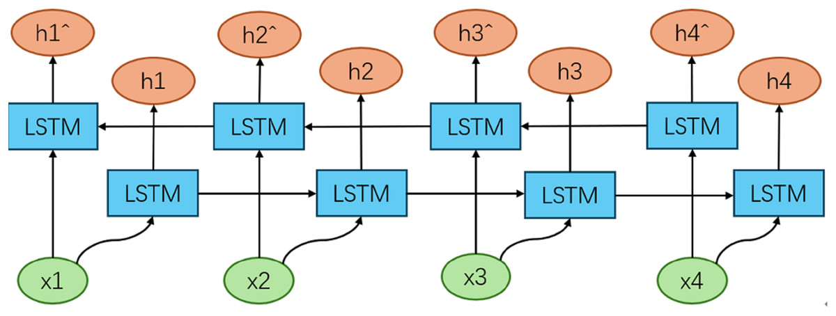
Figure 4: Structure of BiLSTM model.
In this study, the BiLSTM model consists of two separate LSTM layers: one for processing the sequence in the forward direction and another for processing the sequence in the backward direction. Each LSTM layer has an input dimension of 4 and a hidden layer dimension of 4, with two layers in total. The forward LSTM layer processes the input sequence from start to end, capturing forward dependencies, while the backward LSTM layer processes the input sequence from end to start, capturing backward dependencies. The outputs from both LSTM layers are concatenated and fed into a fully connected layer with an output dimension of 1, which generates the final predictions.
-
(4)
LSTM-Attention model
The LSTM-Attention model (Karbasi et al., 2024) synergistically integrates the capabilities of LSTM networks with attention mechanisms to augment the analysis of sequential data. The model’s architecture initiates with an LSTM layer designed to encapsulate temporal dependencies within the input sequence, yielding a succession of hidden states (h1, h2, h3). Subsequently, these states are directed into an attention layer that apportions differential importance to each state, facilitating the model’s ability to prioritize salient information. Following this, the attention-weighted hidden states are projected through a linear layer to produce the ultimate output. The incorporation of an attention mechanism (Neupane, Aryal & Rajabifard, 2024; Mamdouh, Ezzat & Hefny, 2024) within the LSTM framework distinguishes the LSTM-Attention model from conventional LSTM models by endowing selective concentration on specific segments of the input sequence. This feature is particularly beneficial for enhancing the model’s efficacy in applications such as natural language processing and time series prediction, where contextual understanding is paramount. The attention mechanism effectively mitigates a key limitation of standard LSTM models, which uniformly process all time steps, by adaptively modulating focus in accordance with the significance of the input data.
In the LSTM-Attention model, the Attention Layer plays a crucial role. It assigns weights to values using the Attention mechanism, which involves three matrices: the Query, the Key, and the Value. Specifically, when given a Query, the model calculates the correlation between the Query and the Key to select the most appropriate Value based on this correlation. This mechanism allows the model to focus on the most relevant parts of the sequence for generating the final output. In this process, Query, Key, and Value represent different feature vectors: the Query corresponds to the feature vector of subjective awareness, indicating where our attention is focused; the Key corresponds to the vector of a salient feature that identifies the essential information in the data; and Value represents the feature vector of the object itself, which contains the complete details of the data. The architectural of the LSTM-Attention model (Fig. 5).
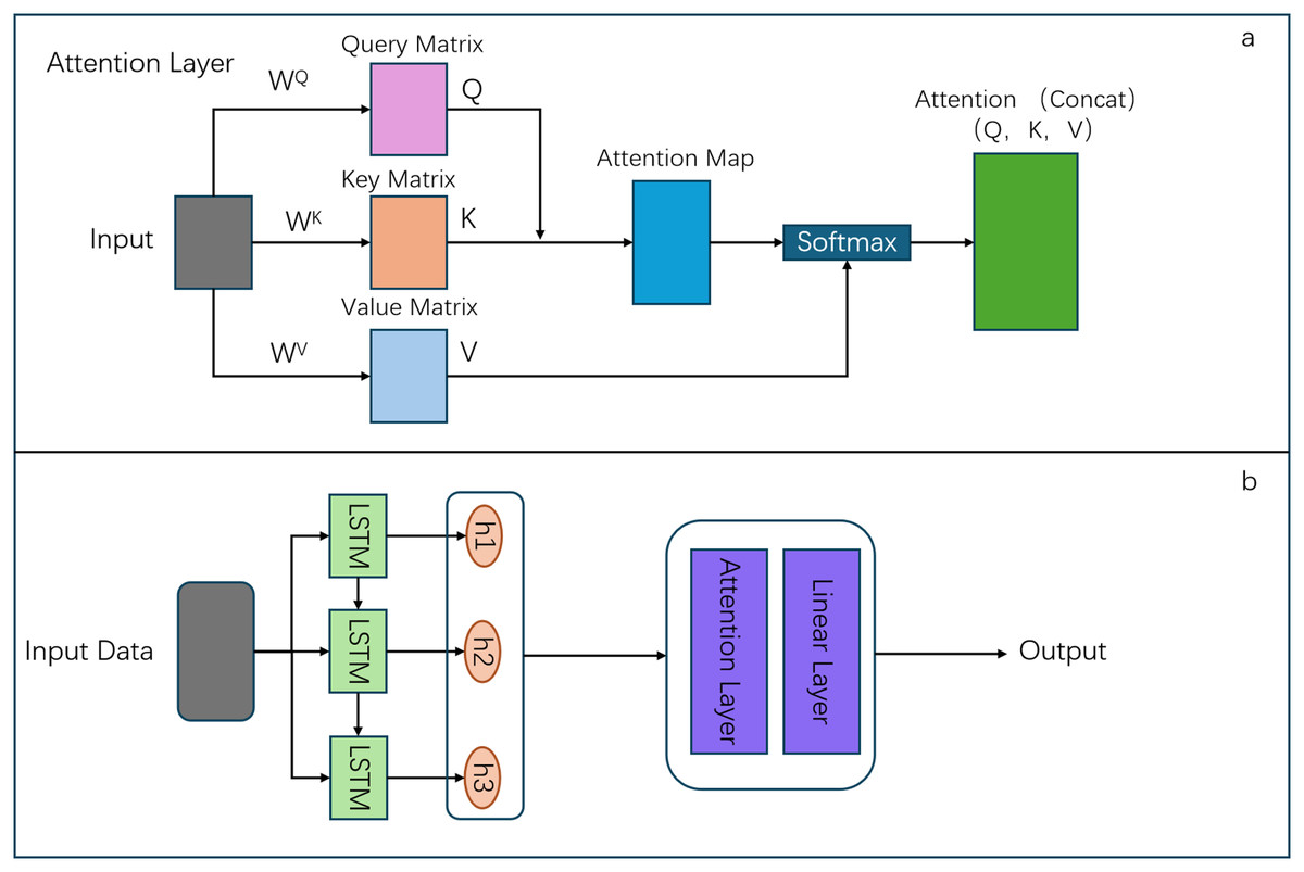
Figure 5: Structure of LSTM Attention model.
In this study, the proposed model architecture integrates an attention mechanism with an LSTM layer to enhance the temporal modeling of sequential data. The LSTM layer, designed with an input dimension matching the feature size, utilizes a hidden layer dimension of 4 with 2 stacked layers, which effectively captures temporal dependencies in the data. The attention mechanism employs three learnable parameter matrices (Wa, Ua, Va) initialized via Xavier uniform distribution, where each matrix has dimensions of (hidden_size, hidden_size). This attention layer computes importance scores through tanh-activated transformations of the LSTM outputs, followed by softmax normalization along the temporal dimension to generate attention weights. The weighted context vector is computed through matrix multiplication between the attention weights and the original LSTM outputs. Finally, the attention-enhanced representations are processed by a fully connected layer with an output dimension of 1 to generate final predictions.
In addition, to rigorously evaluate the performance of the proposed models, we selected three widely recognized metrics in regression analysis: the coefficient of determination (R2), the Root Mean Squared Error (RMSE), and the Mean Absolute Error (MAE). The R2 metric quantifies the proportion of variance in the dependent variable that is predictable from the independent variables, with values closer to 1 indicating a better fit of the model to the data. Conversely, values further from 1 suggest a poorer fit. The RMSE, defined as the square root of the mean squared error, is a widely used metric that is particularly sensitive to outliers due to its quadratic nature. This sensitivity means that large errors can disproportionately influence the RMSE value, making it a stringent measure of model performance, especially when the model is not well-suited to the data. The MAE, which measures the average absolute difference between the predicted and actual values, provides a straightforward and interpretable measure of prediction accuracy. Unlike RMSE, MAE is less sensitive to outliers and offers a more robust measure of central tendency of the residuals. Generally, lower values of RMSE and MAE indicate a better fit of the model to the data, suggesting higher predictive accuracy and reliability.
Finally, it is essential to process data inputs before performing the predictive analyses. We adopted a random sampling approach for data processing (Haq, Jilani & Prabu, 2021; Staudinger et al., 2025), which helps prevent model overfitting and ensures that the model closely aligns with actual data. Specifically, our random sampling method involves shuffling the sequence indices to establish a random order of data samples. Data are then extracted according to the shuffled indices and grouped into sets of four data points. Subsequently, these four data points are used to predict the next data point in the random sequence. This approach is essential for facilitating unbiased learning and enhancing the model’s generalization across diverse conditions. By employing random sampling, we provide the model with a more robust learning environment, thereby improving the accuracy and reliability of predictions.
Results and discussion
Optimal distribution function
Figure 6 shows the locations of the selected grid points and the corresponding Cumulative Distribution Function (CDF) curves, Table 1 presents the distribution of grid points across Shaanxi Province that successfully passed the Pearson Type III distribution test. After a comprehensive evaluation of the CDF curves and the outcomes of the AD test, it has been determined that the Pearson Type III distribution is the most suitable for effectively modeling the GWSA data in subsequent analyses. This choice is based on the distribution’s superior performance in capturing the characteristics of GWSA data, as evidenced by its fitting to the observed data and the statistical validation provided by the AD test.
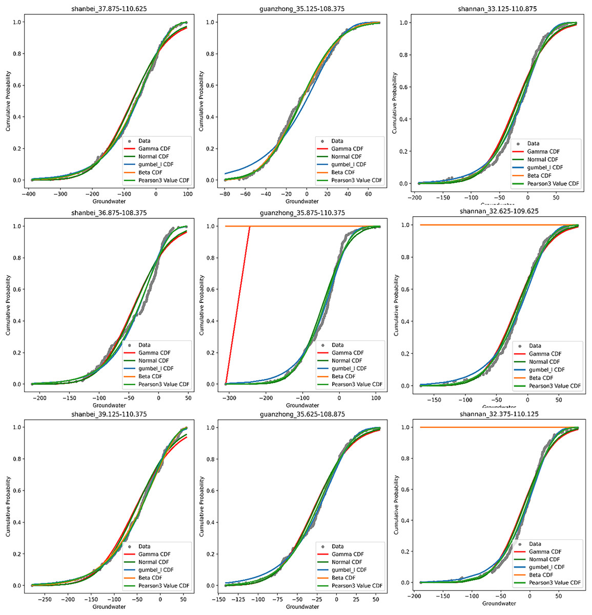
Figure 6: CDF curve fit for three random grid point in the region (Northern Shaanxi, central Guanzhong, and Southern Shaanxi).
| Northern Shaanxi (256) | Central Guanzhong (128) | Southern Shaanxi (192) | |
|---|---|---|---|
| Pearson III | 111 | 99 | 59 |
| Beta | 124 | 101 | 41 |
| Gumbul_L | 63 | 19 | 18 |
Climatic influences on groundwater data fitting in Shaanxi Province
As depicted in Table 1, a considerable number of grid points failed to pass the test. Notably, since 2015, Shaanxi Province has experienced significant changes in groundwater levels, a deteriorating climatic environment, and frequent natural disasters. In July 2015, Northern and Central Shaanxi faced severe drought conditions, exacerbated by widespread high temperatures across the province, leading to hydrological droughts and subsequently groundwater droughts. That summer, many areas in Shaanxi also faced hailstorms. In 2016, Guanzhong and Southern Shaanxi dealt with a prolonged spring drought, which severely impacted the irrigation of food crops. Persistent high temperatures and low rainfall increased reliance on groundwater for irrigation, resulting in a drop in the groundwater level and an elevated risk of groundwater droughts. In 2017, Shaanxi Province encountered dual natural disasters of heavy rainfall and drought on several occasions. In July, Northern Shaanxi received substantial rainfall, whereas Guanzhong and Southern Shaanxi suffered from severe ambient drought, despite increased rainfall in March. July 2018 brought widespread heavy rain and storms, particularly in north-central Shaanxi, western Guanzhong, and western and Southern Shaanxi, with torrential downpours occurring in Southern Shaanxi in August. Throughout that summer, the province also endured widespread and long-lasting hot weather. From August to September 2019, Northern Shaanxi, central Guanzhong, and Southern Shaanxi experienced heavy rainfall and storms, while most of the province faced severe drought in March and April. This included moderate to severe meteorological droughts occurring in Northern Shaanxi, east-central Guanzhong, and eastern Southern Shaanxi. July saw sustained high temperatures, with thermometers exceeding 37 °C and occasionally surpassing 40 °C. In August 2020, Shaanxi Province experienced frequent heavy precipitation processes from south to north, while late spring and early summer were marked by low rainfall and drought conditions, particularly severe drought in Northern Shaanxi, ranging from severe to exceptional. These extreme weather events led to drastic fluctuations in groundwater levels, resulting in outliers that negatively impacted the accuracy of subsequent calculations and made it challenging to select a suitable fitting function for data analysis.
We found that fitting groundwater data was particularly challenging in Northern and Southern Shaanxi. This may be attributed to the specific geographic locations and climatic conditions of these regions. Northern Shaanxi is characterized by a temperate continental monsoon climate with sparse rainfall, which essentially contributes to the region’s drought and anomalous GWSA values. As Northern Shaanxi is already affected by drought and has limited river systems, these conditions further complicate the data fitting process. In contrast, the Guanzhong region experiences a warm temperate semi-humid and semi-arid climate (Zhong et al., 2018; Talebi, Torabi & Daneshpour, 2024) with more abundant rainfall, moderate temperatures, and fewer extreme weather events. These favorable conditions result in relatively stable GWSA changes, making it easier to find a suitable function for data fitting. Southern Shaanxi, located immediately south of the Qinling Mountains, falls within the subtropical continental monsoon climate zone. The Han River flows through the region from west to east, and it borders Southern areas such as Sichuan and Chongqing. The warm and humid climate of Southern Shaanxi, with its plentiful rainfall, leads to more significant fluctuations in the water table with increased precipitation and warmer temperatures. This variability increases the frequency of outliers, resulting in fewer data points that can be successfully matched when fitting the function distribution in Southern Shaanxi. Overall, these climatic and geographical factors significantly influence the effectiveness and difficulty of fitting groundwater data across different regions.
Comparison of GWSA and their correlation with climatic conditions
Guanzhong region has the highest number of grid points that passed in the AD test compared to the Northern and Southern regions of Shaanxi. This phenomenon can be attributed to the relatively mild climatic conditions in Guanzhong, where changes in groundwater levels are relatively smooth and infrequent, resulting in less drastic fluctuations in GWSA. In contrast, Northern Shaanxi has long experienced severe drought conditions, while Southern Shaanxi frequently faces persistent high temperatures and extreme weather events, such as heavy rainfall and storms. These factors contribute to more drastic changes in GWSA in these two regions. This indicates that the climatic characteristics and environmental conditions of different significantly impact the stability of GWSA data and the selection of appropriate prediction models.
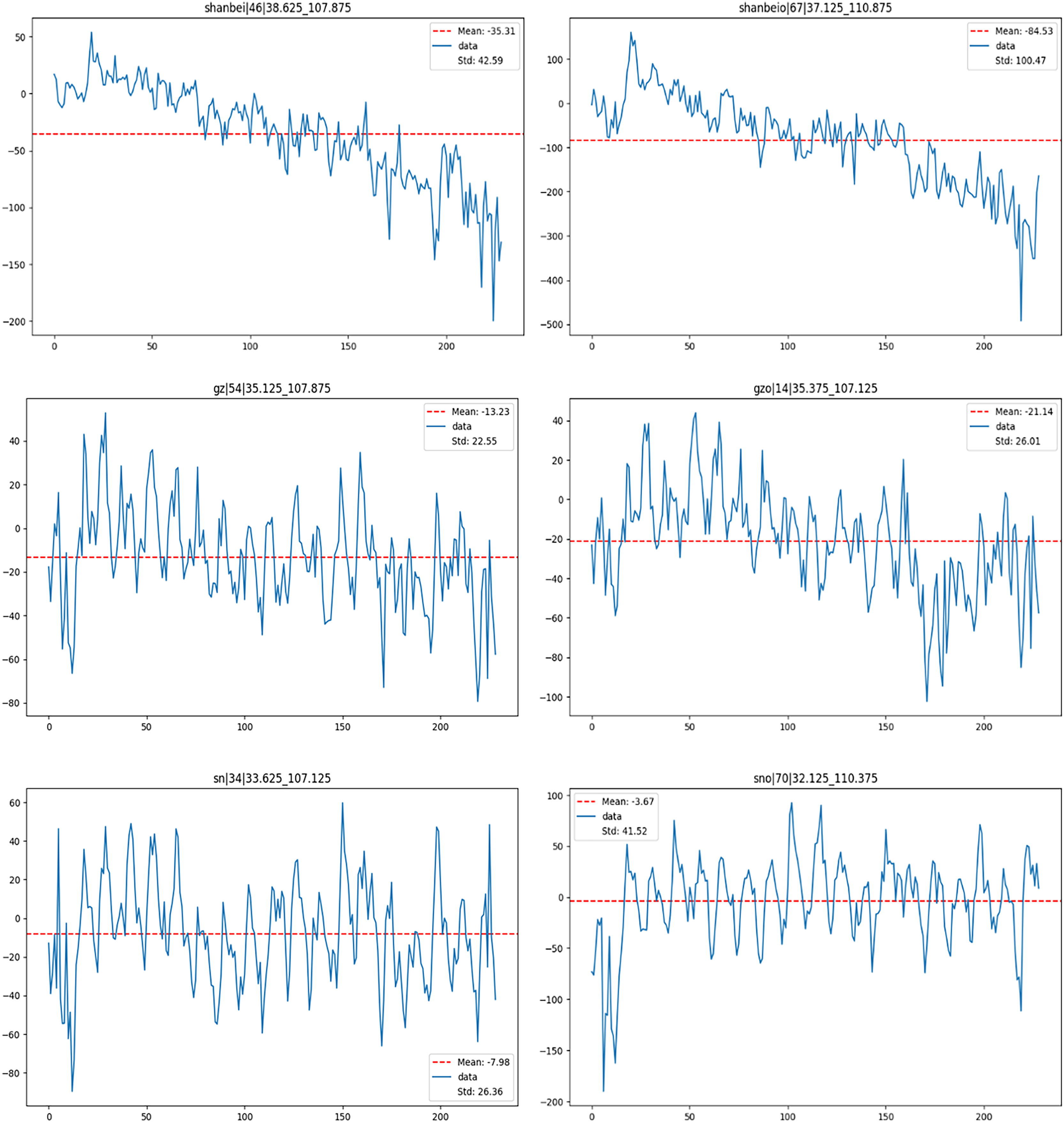
We chose one grid point that passed the AD test and one that did not, from each of the Northern Shaanxi, Guanzhong, and Southern Shaanxi regions for the observation of GWSA data. Figure 7 illustrates the distribution of GWSA and its change patterns across areas of Shaanxi Province. By analyzing the GWSA change graph, we can highlight the difference between the grid points that passed the test and those that did not. The untested ones tend to exhibit outliers, which is why they are less amenable to precise fitting compared to the tested ones. The left side of the figure shows the tested grid point and the right side displays the untested grid point.
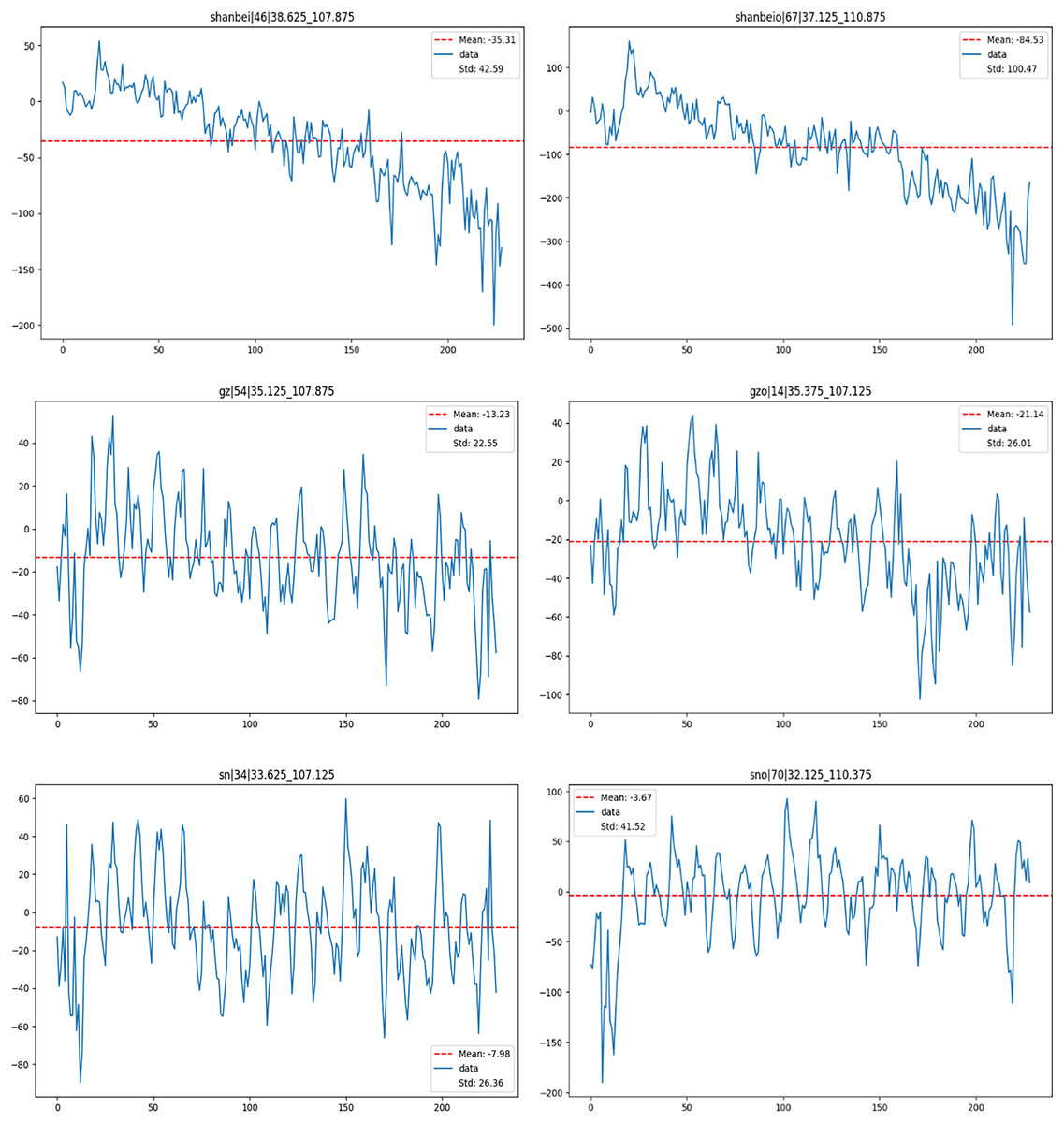
Figure 7: Map analyzing changes in groundwater storage in different regions (passing points on the left and non-passing grid point on the right).
In the Northern Shaanxi region, GWSA values for grid points that passed the AD test range from −200 to 50, whereas those for points that failed the test range from −500 to 100. The mean and standard deviation for the passing grid points are −35.31 and 42.59, respectively; for the failing points, these values are significantly higher at −84.53 and 100.47, respectively. This comparison indicates that the passing data set shows less fluctuation, suggesting higher consistency, while the failing set exhibits more variability, with some deviation from the overall trend. The overall trend of GWSA in Northern Shaanxi is decreasing, signifying a reduction in groundwater levels and an aggravation of drought conditions. The decline in GWSA among the tested grid points is relatively minor. However, there are significant differences in drought conditions among grid points in Northern Shaanxi, where extreme events may induce particularly severe drought conditions at certain points, leading to substantial data fluctuations. These findings provide valuable insights into groundwater drought conditions in Northern Shaanxi and underscore outliers that require focused analysis in data fitting and trend analysis.
In the Guanzhong region, characterized by a temperate monsoon climate with hot and rainy summers and cold, dry winters, the climate is relatively mild, resulting in minor fluctuations in precipitation and temperature. As a consequence, the GWSA values exhibit a relatively narrow range. Specifically, the GWSA values for grid points that passed the AD test range from 40 to −80, whereas those that failed the test range from 40 to −100. The mean values for the passing and failing groups are −13.23 and −21.14, respectively, with standard deviations of 22.55 and 26.01, respectively. These statistics indicate that the data that passed the AD test demonstrate greater stability. In contrast, the data that did not pass the test display more significant variability. The general decreasing trend in GWSA, accompanied by fluctuations, corresponds with the climatic characteristics of the Guanzhong region. These variations are likely influenced by extreme climatic events, including extremely high temperatures and heavy rainfall, which may adversely affect the groundwater system. Additionally, the tested grid point exhibit a lower frequency of outliers in GWSA compared to the untested ones, suggesting that a higher incidence of anomalous events may complicate the process of identifying a suitable model for the data.
In the Southern Shaanxi region, GWSA values for grid points that passed the AD test range from 60 to −80, while those for grid points that did not pass the test span a broader range, extending from 100 to −200. The mean values for these two sets of grid points are −7.98 and −3.67, respectively, with standard deviations of 26.36 and 41.52, respectively. This suggests that the data not passing the test exhibit greater fluctuations and a higher frequency of outliers compared to the data that passed the test. Extreme weather events, such as high temperatures and heavy rainfall, are common in Southern Shaanxi and contribute to the recurring fluctuations observed in the GWSA.
The findings underscore a strong correlation between the GWSA and climatic conditions in the region, highlighting the potential impacts of extreme weather on the groundwater system.
Combining SGI and deep learning methods to analyze drought conditions
Table 2 presents a comprehensive comparison of the performance of the four deep-learning models. The analysis of the performance metrics reveals several important insights. The CNN-LSTM model demonstrates the highest R2 value of 0.88, indicating its superior ability to explain the variations in the drought index. This suggests that the CNN-LSTM model captures the underlying patterns in the data more effectively than the other models. Additionally, both the CNN-LSTM and LSTM-Attention models achieve the lowest RMSE values at 0.32, highlighting their effectiveness in controlling prediction errors. This is further supported by the MAE metrics, which confirm that these two models exhibit the best overall performance. These findings suggest that the CNN-LSTM and LSTM-Attention models are particularly well-suited for predicting the groundwater drought index, offering a balance between accuracy and robustness.
| R2 | RMSE | MAE | |
|---|---|---|---|
| LSTM | 0.84 | 0.36 | 0.24 |
| CNN-LSTM | 0.88 | 0.32 | 0.16 |
| BiLSTM | 0.86 | 0.34 | 0.20 |
| LSTM-Attention | 0.87 | 0.32 | 0.16 |
Although GRACE directly provides measurements of GWSA, the physical units of these measurements—such as centimeters of equivalent water height—pose challenges for comparing drought intensity across different regions and time periods. To address this limitation, we will employ the SGI. The SGI enables a more standardized and comparable assessment of drought frequency and severity, thereby facilitating a more robust analysis of groundwater drought conditions.
After selecting the Pearson Type III function as the best-fitting model to estimate the SGI, we conducted a further analysis of the SGI data. This involved applying the MK trend test to evaluate the SGI trend and infer drought trends in each region. The MK trend test categorizes the trend into three types: increasing, decreasing, and no trend. The P-value from the test results indicates the significance of any trends in the data; a P-value less than 0.05 signifies a significant trend. In contrast, the s-value indicates the direction of the trend: an s-value greater than zero implies an increasing trend, while an s-value less than zero indicates a decreasing trend.
Analyzing Table 3, it is observed that the SGI values from all grid points in Northern Shaanxi demonstrate a clear and pronounced decreasing trend. This trend suggests that drought conditions in Northern Shaanxi are continuing to worsen. In the Guanzhong region, the situation is more complex; while several grid points show a decreasing trend, others do not exhibit any significant trend. Specifically, 112 grid points show a clearer downward trend, whereas 16 grid points show no notable trend. The data suggest that the drought situation in Guanzhong is also severe and gradually worsening. In Southern Shaanxi, drought conditions exhibit more variability: 95 grid point show a significant increasing trend in SGI values, 38 show a significant decreasing trend, and 59 show an insignificant trend. These findings highlight substantial differences in drought conditions across various regions of Southern Shaanxi.
| Increasing | Decreasing | No trend | P | S | |
|---|---|---|---|---|---|
| – | – | – | – | – | |
| Northern Shaanxi | – | 256 | – | <0.05 | <0 |
| – | – | – | – | – | |
| – | – | – | – | – | |
| Central Guanzhong | – | 112 | – | <0.05 | <0 |
| – | – | 16 | >0.05 | – | |
| 95 | – | – | <0.05 | >0 | |
| Southern Shaanxi | – | 38 | – | <0.05 | <0 |
| – | – | 59 | >0.05 | – |
The analysis of the SGI index reveals distinct dynamics of groundwater drought in each region. In Northern Shaanxi, groundwater drought is significantly influenced by climatic and environmental factors, as this region is classified as arid or semi-arid. The region experiences low rainfall and high evaporation rates, which limit the recharge of groundwater resources. The uneven distribution of water resources, coupled with a high dependence on groundwater for agricultural, residential, and industrial use, has led to overexploitation, further exacerbating the drought problem and its progressive deterioration over the years. In contrast, the Guanzhong region, characterized by its relatively flat terrain, mild climate, and abundant rainfall, faces its own set of challenges. The region, home to the Weihe River Plain, relies heavily on water resources due to agricultural and industrial development, resulting in excessive groundwater extraction, particularly during the hot summer months. However, Guanzhong benefits from its proximity to the Wei River, allowing for some groundwater recharge through river inflows and precipitation. On the other hand, Southern Shaanxi is renowned for its humid climate and ample rainfall, leading to relatively abundant water and forest resources. Groundwater reserves in this region account for 49.7% of the province’s total groundwater supply. Agricultural, industrial, and domestic demands heavily rely on these groundwater supplies. The region benefits from sufficient precipitation, ensuring adequate groundwater recharge. Additionally, low population density and high forest cover contribute to the conservation of these resources.
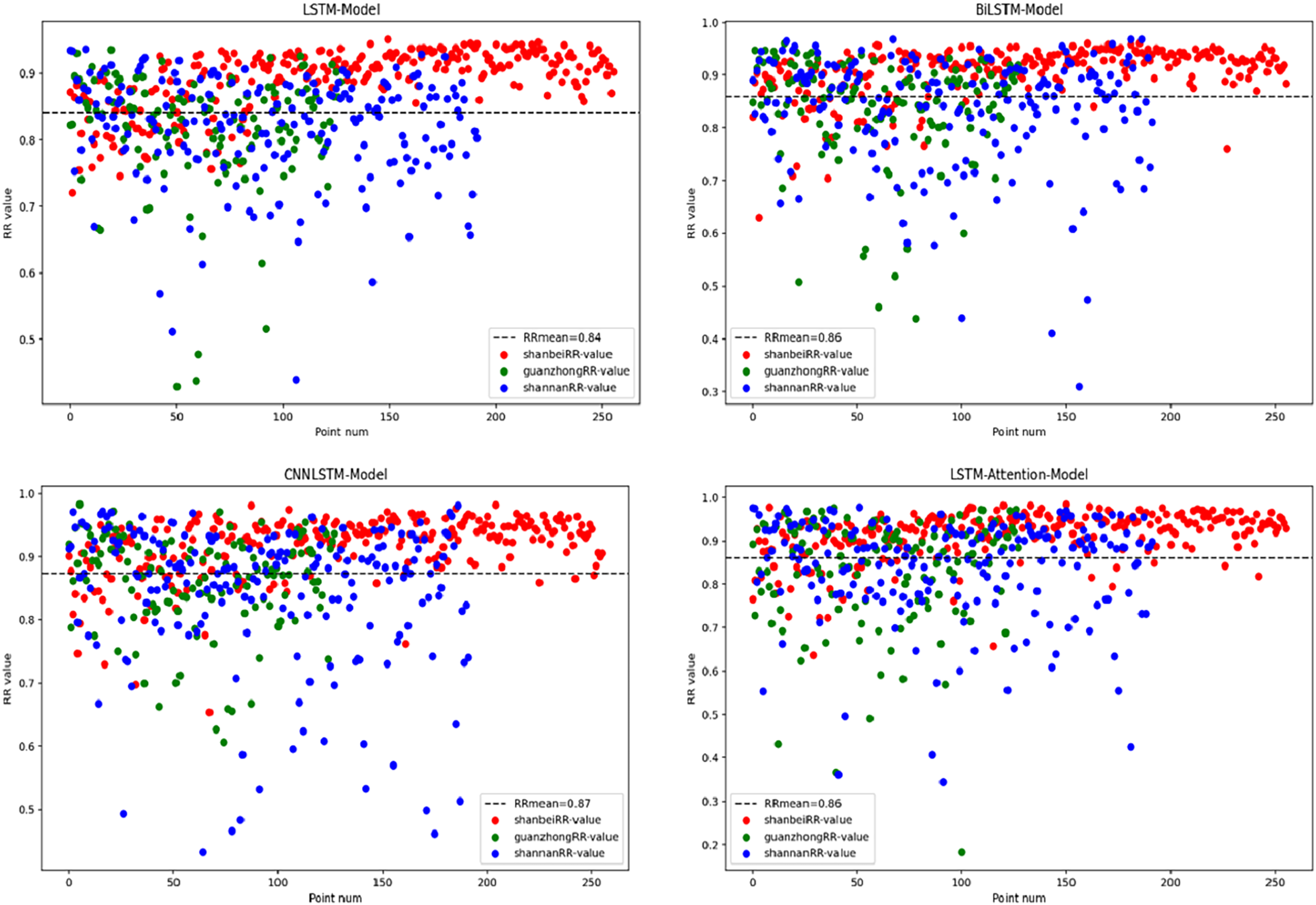
Therefore, analyzing the dynamics of the SGI is crucial for our objectives (Bi et al., 2024). Deep learning techniques have been widely applied in various fields and show great potential in hydrology. In this study, we selected and compared four popular deep learning models: LSTM, BiLSTM, CNN-LSTM, and LSTM-Attention. We assessed their accuracies in predicting the drought index (Afan et al., 2021) (Fig. 8) to determine the most suitable model for drought index prediction. Figure 8 illustrates that, despite variations among the models, their performance in predicting the SGI across different regions is generally similar. The prediction performance indexes clustered between 80% and 90% for most of the grid points in the three areas studied. By comprehensively evaluating the prediction accuracies of the 576 grid points, we found that the LSTM model had an average accuracy of 84%, which was relatively low compared to the other models. The BiLSTM and LSTM-Attention models also showed lower prediction accuracies for individual observations; however, their average accuracies improved, reaching 86% and 87%, respectively. Compared to the other models, the CNN-LSTM model performed best in drought index prediction, achieving an average accuracy of 88%. This remarkable achievement is attributed to its deep learning algorithm, which enables the model to automatically learn and adapt from the input data to generate predictive outputs. The strength of the CNN-LSTM model lies in its ability to automatically identify and extract complex features from the data, significantly reducing the challenges encountered when manually selecting drought predictors and managing spatial-temporal variability in the traditional approaches. This indicates a notable enhancement in the predictive performance of these improved LSTM models compared to the original LSTM models.
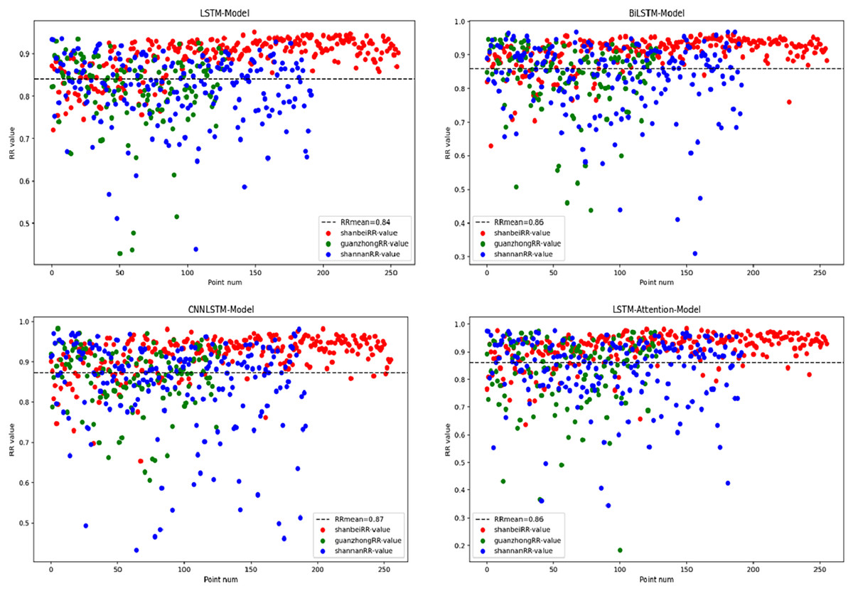
Figure 8: Performance plot of the four models in predicting the SGI for all grid point.
Our results reveal that the prediction performance of all models is particularly strong in the Northern Shaanxi region. Specifically, the prediction accuracies of grid points in this area are primarily within the range of 80% to 90%, showing the high reliability of the models. In contrast, the model performance in Guanzhong and Southern Shaanxi regions is slightly deficient, with grid points there showing greater fluctuations in error. This discrepancy may stem from the more complex and variable climatic conditions in these regions, which can include extreme climatic events, such as heavy rainfalls and droughts. These factors introduce additional uncertainties and challenges when predicting the groundwater drought index.
To improve the accuracy of forecasts for Guanzhong and Southern Shaanxi, future work should consider the specific climatic factors of these regions in greater detail. This may involve adapting and optimizing the model to better align with the climatic characteristics of these areas. By doing so, we can expect to improve the model’s prediction performance in these critical regions, thereby providing more accurate and reliable data to support drought monitoring and early warning systems.
Based on the model performance metrics and their corresponding prediction results, the CNN-LSTM model demonstrates the best performance in drought-index forecasting. Given its high R2 value, low RMSE, and optimal MAE, the CNN-LSTM model effectively balances accuracy and robustness, making it the most suitable choice for this task.
The study by Haq, Jilani & Prabu (2021) has demonstrated the significant potential of LSTM models in predicting groundwater levels. Therefore, exploring variants of the LSTM model became the primary objective of our research. Our results indicate that the CNN-LSTM model outperforms the traditional LSTM model in predictive performance. Moreover, by integrating the SGI with deep learning, we have proposed a more standardized method for drought assessment. This framework not only enhances the accuracy of assessing drought frequency and severity across different regions and time periods but also provides a solid foundation for drought monitoring and early warning systems. Future research could further improve model accuracy and applicability by incorporating higher-resolution data sources and exploring other advanced deep learning models.
Conclusions
In this study, we utilized the SGI, which is derived from the SPI, to conduct a comprehensive assessment of groundwater drought in Shaanxi Province. By using GRACE data, we estimated the groundwater storage in three regions: Northern Shaanxi, Guanzhong, and Southern Shaanxi, and analyzed the spatial and temporal evolution characteristics of 576 grid points. The findings indicate that changes in groundwater storage exhibit significant regional differences within Shaanxi Province. The SGI index inherits both the strengths and weaknesses of SPI, making it critical to select a suitable distribution function for accurate SGI calculations. Our analysis of the groundwater drought situation in each region demonstrated that the SGI index effectively reflects local groundwater drought conditions. Further trend analysis of the SGI index using the MK trend test reveals that changes in its trend are closely related to regional characteristics, confirming the applicability of the SGI as an SPI-derived index for assessing groundwater drought. By predicting the SGI index, we can monitor and prevent future groundwater drought events, providing a scientific basis for the sustainable management and protection of groundwater resources. This study also explores applying deep learning techniques in predicting the SGI index by selecting four models: the LSTM, BiLSTM, CNN-LSTM, and LSTM-Attention. The results of the study show that:
The Pearson III function was found to be the most appropriate after evaluating the Pearson III, Beta, Gumbel, Normal, and Polar distribution functions for the AD test.
Analysis of the SGI indicates that trends in the drought index align with regional groundwater drought conditions.
Among the four deep learning models, the CNN-LSTM model demonstrates the best performance in predicting the SGI index, yielding strong overall results.
The findings of this study hold significant practical implications for the understanding and management of groundwater drought conditions in Shaanxi Province. The accurate prediction of the SGI index provides a robust basis for decision-making in water resource management, agriculture, and disaster preparedness. By offering early and precise warnings of impending groundwater droughts, stakeholders are empowered to implement timely interventions that can effectively mitigate the impacts of drought on ecosystems, agriculture, and human activities.
The application of deep learning models in groundwater drought research is both forward-looking and pragmatic. Utilizing this technology for groundwater drought prediction represents a promising approach and offers a novel method for the scientific and rational detection and prevention of groundwater drought events. This not only facilitates the sustainable management of groundwater resources but also enhances their protection.