
Node disjoint path construction algorithm in the folded divide-and-swap cube
- Published
- Accepted
- Received
- Academic Editor
- Michele Pasqua
- Subject Areas
- Algorithms and Analysis of Algorithms, Distributed and Parallel Computing, Optimization Theory and Computation, Scientific Computing and Simulation, Theory and Formal Methods
- Keywords
- Node-disjoint path, Folded divide-and-swap cube, Interconnection network
- Copyright
- © 2026 Gao et al.
- Licence
- This is an open access article distributed under the terms of the Creative Commons Attribution License, which permits unrestricted use, distribution, reproduction and adaptation in any medium and for any purpose provided that it is properly attributed. For attribution, the original author(s), title, publication source (PeerJ Computer Science) and either DOI or URL of the article must be cited.
- Cite this article
- 2026. Node disjoint path construction algorithm in the folded divide-and-swap cube. PeerJ Computer Science 12:e3458 https://doi.org/10.7717/peerj-cs.3458
Abstract
The folded divide-and-swap cube FDSCn (n = 2d, d ≥ 1) is a new hypercube variant, which has many superior properties compared to the hypercube. FDSCn is suitable as a candidate topology for data center networks. In this article, we investigate the one-to-one node disjoint path problem of FDSCn. We first present an algorithm to construct a path between any two distinct nodes u and v based on the structural characteristics of FDSCn. Then we develop an algorithm to build d + 2 node disjoint paths between any two different nodes in FDSCn, and show that the maximum length of these paths shall not exceed n + 9.
Introduction
Supercomputers are high-performance computing systems that can perform complex tasks at an unprecedented speed. These systems typically consist of thousands or even millions of processors. An interconnection network, which is the fundamental topological structure of a supercomputer, plays a vital role in the performance of a supercomputer. The topology structure of an interconnection network is always modeled with a graph , where is the processor set and is the set of communication links connecting these processors. In a graph, a path is a sequence of distinct vertices such that each pair of consecutive vertices and is connected by an edge in , where . The length of a path P, denoted by , is the number of edges it contains. The distance between two vertices and , denoted by , is the length of the shortest path connecting them. The diameter of G is the maximum distance between any two vertices in G. A vertex is a neighbor of if there exists an edge . The neighborhood of , denoted by , is the set of all neighbors of . Let . Then and and . In this work, the terms “vertex” and “node” are used interchangeably.
One-to-one node-disjoint paths between any two distinct nodes and in a graph refer to a set of paths that do not share any common nodes except the end nodes and . Since each path is independent with the other ones, node-disjoint paths allow data to be transmitted through multiple paths. In distributed computing systems, node-disjoint paths are essential for fault-tolerant communication between different nodes. By using multiple disjoint paths, supercomputers can continue to function properly even when some nodes become unavailable due to hardware failures or network issues. There are many works on disjoint path problem in hypercubes (Saad & Schultz, 1988), crossed cubes (Kulasinghe, 1997), twisted cubes (Chang, Wang & Hsu, 1999), m bius cubes (Kocik & Kaneko, 2017), balanced hypercubes (Cheng, Hao & Feng, 2014; Liu et al., 2024), folded hypercubes (Lai, 2021; Liu, 2010), bcube (Fan et al., 2023), -ary -cube networks (Lv et al., 2024), enhanced hypercubes (Ma, Guo & Li, 2022), dcell networks (Wang et al., 2016), dragonfly networks (Wu et al., 2022), and alternating group graphs (You et al., 2015).
The -dimensional hypercube which has network cost is one of the most important interconnection networks. The divide-and-swap cube is a newly proposed hypercube variant, which reduces the network cost to (Kim et al., 2019), while and have the same number of nodes. To reduce the diameter of , the folded divide-and-swap cube is proposed. The upper bounds of diameters of and are and ( ), respectively (Kim et al., 2019). Both and are hierarchical networks. Besides, and are Hamiltonian and Hamiltonian-connected. Chang et al. (2021) pointed out that is suitable as a candidate topology for data center networks, and they proposed a recursive construction of a dual-CIST for . Zhao & Chang (2023) investigated the generalized connectivity on . Zhou et al. (2024) determined the -extra connectivity of the divide-and-swap cube . has a node degree of , which is much lower than most of the hypercube variants. Lower node degree reduces hardware costs, as it requires fewer ports per server/switch, minimizing the expense of network adapters and cabling. has the smallest network cost among all hypercube variants, which proves ’s superiority in balancing performance and resource usage. Besides, exhibits double exponential scalability, which surpasses many traditional interconnection topologies (e.g., bcube, dcell) and meets the demand for connecting massive numbers of servers in modern data centers.
In this work, we investigate the one-to-one node disjoint path problem of . Let and be any two distinct nodes in where and . We give an algorithm to construct disjoint paths between and . The main contributions of this work are shown as below:
We present an algorithm QP to construct a path between any two distinct nodes and based on the structural characteristics of . This algorithm can quickly locate the subgraph where these two vertices are located, thereby reducing the scale of the path constructing problem.
We develop an algorithm O2OMain to build disjoint paths between any two different nodes in and show that the maximum length of these paths shall not exceed .
Preliminaries
In this section, we give the formal definition of and . Each node in is denoted by an -bit binary string, where with for . is defined as follows.
Definition 1. (Kim et al., 2019) For any integers and , has nodes, each of which is represented by an -bit binary string, where and with . For each with , , and . If , then and is empty. If node satisfies one of the following conditions, then .
-
(1)
, where is the complement of . Here, is called an -edge.
-
(2)
Here, is called an -edge.
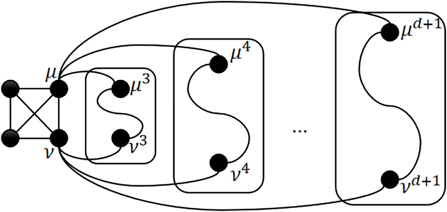
and are shown in Fig. 1. Each node in has neighbors. Hence, is -regular. If is connected to with an -edge, then we call the 1-neighbor of , denoted by ; If is connected to with an -edge ( ), then we call the -neighbor of , denoted by , where (See Table 1).
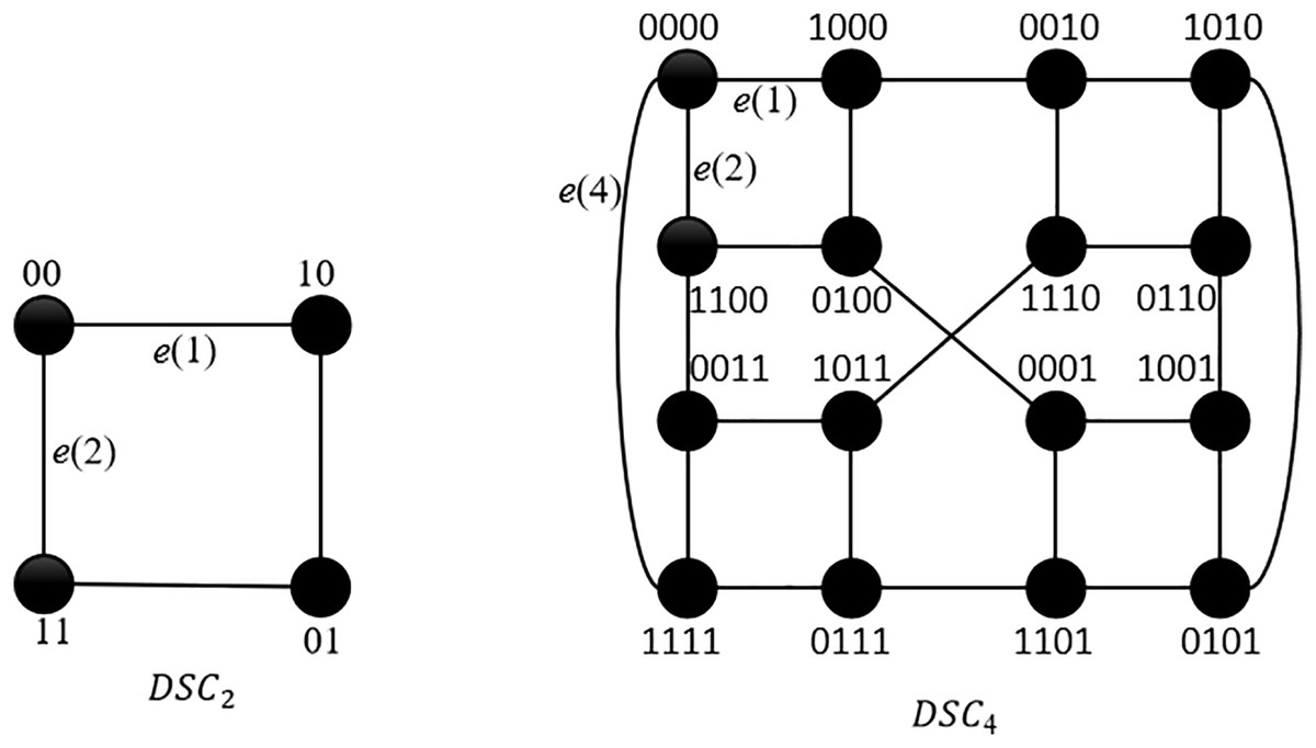
Figure 1: and .
| Symbols | Values | ||||
|---|---|---|---|---|---|
Definition 2. Let be a specific ( − )-digit binary string where and . Define as a subgraph of induced by is a -digit binary string}. We call an embeded of with the identifier .
For example, is an embeded induced by in Fig. 1, where 00 is the identifier. The rightmost 2-digit binary string of each node in is same, which is 00. Let with . According to Definition 2, node belongs to . For two different nodes and of , if the rightmost ( − )-digit binary strings of and are same, or only the leftmost -digit binary strings of and are different, then and belong to the same . In this work, we say that is an embeded subgraph of its own, where the identifier is empty.
From Table 1, we can see that only the leftmost -digit binary strings of and are different. Hence, and are in the same embeded . In this work, in order to simplify the expression, we may omit the identifier of the embeded subgraph sometimes.
Next, we give the definition of . For any integer with and , is built based on by adding an edge to each node of . Hence, is -regular.
Definition 3. (Kim et al., 2019) , , where and . An edge in is called an -edge.
If is connected to with an -edge, then we call the 0-neighbor of , denoted by . and are shown in Fig. 2. By the definition of , the concept of embeded subgraph can also apply to . Hence, we have the following properties:
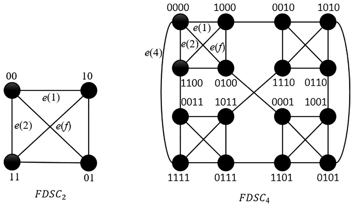
Figure 2: and .
Property 1. For any node with and , there exist the following properties:
-
(1)
If the rightmost ( − )-digit binary strings of and are the same, or only the leftmost -digit binary strings of and are different where , then and are in the same embeded .
-
(2)
has neighbors in the embeded of , where .
-
(3)
, , and are in the same embeded .
Suppose is an embeded subgraph of , where and . The direct subgraph of D is callled a module of D. D can be decomposed into embeded subgraph , each of which is a module of . For example, in Fig. 3, suppose , then D can be decomposed into embeded . Let , where is the address in a module and is the address of the module in D. For example, in Fig. 3, suppose , then are the module addresses of the embeded in D. Suppose , then are the module addresses of the four embeded in D. Each module in is denoted by where ( ) is the module address. Each node in has interior neighbors inside and is the external neighbor outside . Any two distinct modules in D are connected by at least one edge, which is called a bridge edge.
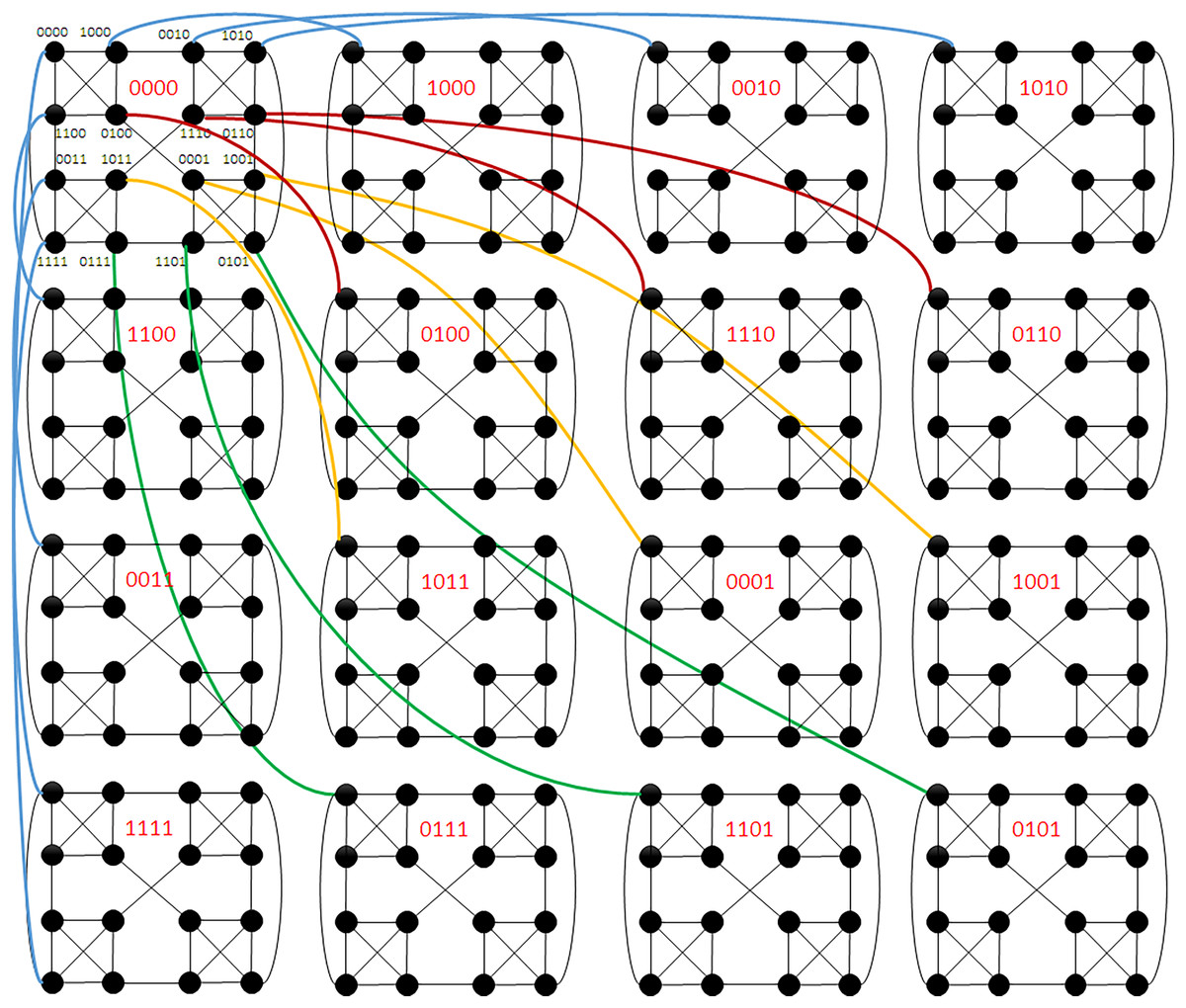
Figure 3: A partial view of .
Property 2. (Kim et al., 2019) For any two distinct modules and in with identifier B where and , there exist the following properties:
-
(1)
if , then there is one bridge edge between modules and .
-
(2)
if , there are two bridge edges and between modules and .
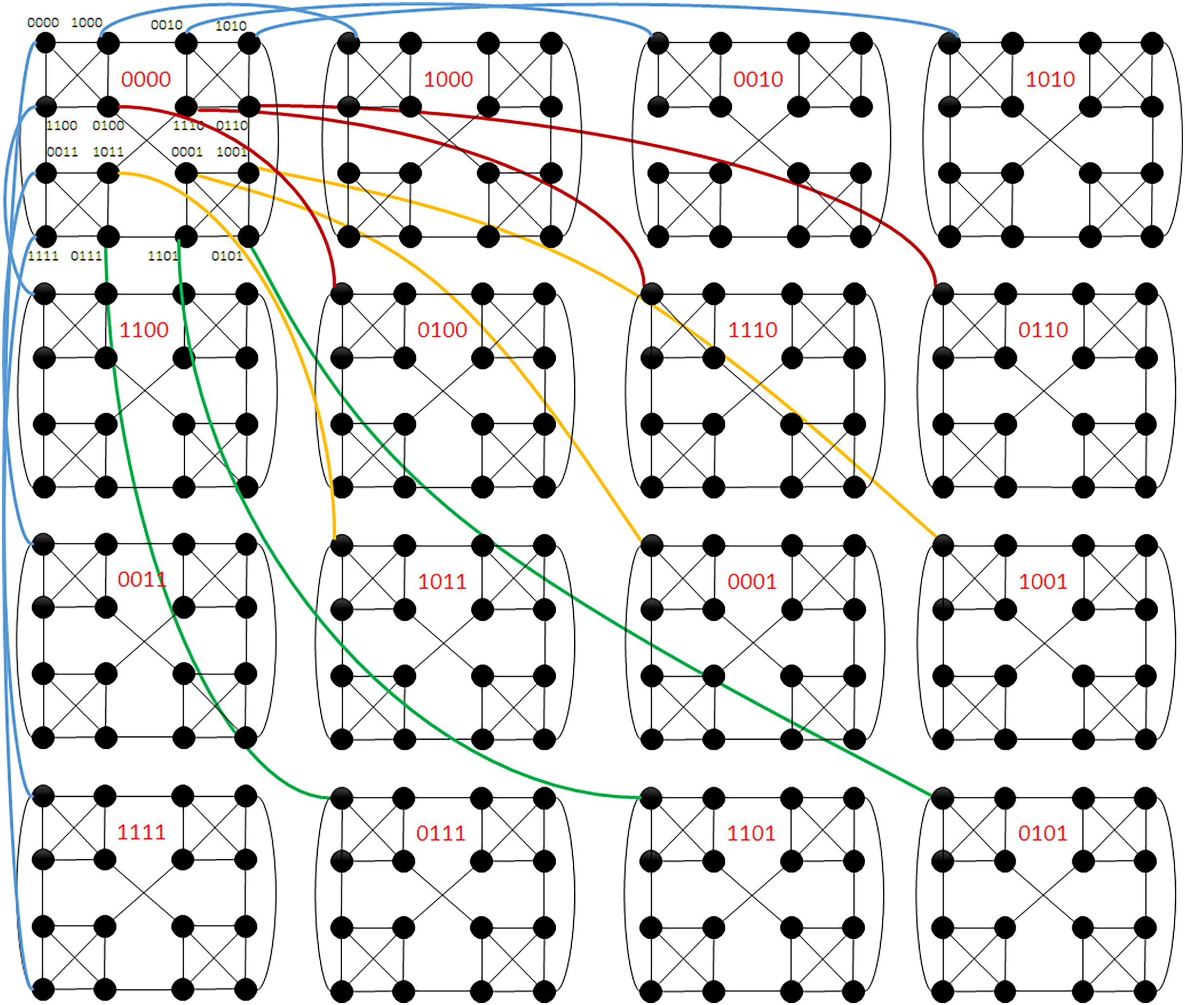
For example, in Fig. 3, suppose . For modules and in D, there are two bridge edges (00000000, 11111111) and (11110000, 00001111). For modules and in D, there is one bridge edge (00001000, 10000000). Suppose . For modules and in D, there are two bridge edges (00000000, 11110000) and (11000000, 00110000). For modules and in D, there is one bridge edge (01000000, 00010000).
Let and be two distinct nodes in different modules and of the same where . Then, is the module address of , and is the module address of . If we replace the first bits of with to obtain node , and replace the first bits of with to obtain node , then is a bridge edge between and .
For example, in Fig. 3, suppose , and with . Then is in module with and is in module with . If we replace the first 2 bits of with , then we get node . And if we replace the first 2 bits of with , then we get node . Then, (01000000, 00010000) is a bridge edge between and . We list some acronyms and notations in Table 2, which will be used in this work.
| Symbol | Definition |
|---|---|
| An -dimensional folded divide-and-swap cube | |
| An embeded subgraph of | |
| A direct embeded subgraph of or a module of | |
| The interior neighbor set of inside the where lies | |
| The external neighbor of in outside the where lies | |
| The module which node is connected to | |
| The module set |
Construction of a path between any two distinct nodes in
In this section, we will give two basic algorithms which will be used to build a path between any two distinct nodes in . Let and be any two distinct nodes in and with . If exists, then and . By Property 1(1), and are in the same embeded . Otherwise, and are in the same embeded .
If and are in the same embeded where , then they are also in the same embeded . For example, suppose and . Then these two nodes are in the same , and we can also consider that and are in the same . Hence, is the minimum common dimension of the embeded subgraph where and lie. We give an algorithm to get the minimum common dimension for and as follows.
As shown in Fig. 3, for nodes and where , since , then algorithm MinCommonDimension returns 3. Hence, is the minimum common dimension of the embeded subgraph, and , are in the same embeded . For nodes and where , since and , then algorithm MinCommonDimension returns 2, and , are in the same embeded . For nodes and where , since and , then algorithm MinCommonDimension returns 1, and , are in the same embeded .
Next, we use a recursive algorithm to build a path between any two different nodes. Let and be any two distinct nodes in . If and are in the same embeded , then is the required path. If and are in the same embeded where is the minimum common dimension of the embeded subgraph in which and lie, then and are in different s. We select nodes and where and , and are in the same respectively, and is the bridge edge connecting these two . For nodes and , and , we use the same method to build the paths between them. Therefore, we can adopt a recursive construction approach to build the path between and . The detailed algorithm is shown as below.
Each node exists in a certain embeded subgraph. In line 1, we get the minimum common dimension of the embeded subgraph where and lie with Algorithm 1; In lines 2–4, if and exist in the same , we return the required path , since is a complete graph. If and lie in the same embeded , we need to get the bridge edge which connects the s where and lie. In line 5, we get node by replacing of with of . In line 6, we get node by replacing of with of . Then, is the required bridge edge.
| Input: Nodes , , and |
| Output: an integer k where 2k is the minimum common dimension of the embeded subgraph in which μ and ν lie. |
| 1: for do |
| 2: if then |
| 3: ; |
| 4: return k; |
| 5: end if |
| 6: end for |
| 7: return ; |
| Input: Nodes , and . |
| Output: a path P between μ and ν in FDSCn. |
| 1: ; |
| 2: if then |
| 3: return “,” ; |
| 4: end if |
| 5: |
| 6: |
| 7: if then |
| 8: if then |
| 9: “,” ; |
| 10: else |
| 11: “,” ; |
| 12: end if |
| 13: else |
| 14: if then |
| 15: “,” ; |
| 16: else |
| 17: “,” ; |
| 18: end if |
| 19: end if |
| 20: return P; |
As shown in Fig. 3, for nodes and where , , , and . In this case, . Then, we have , and is the bridge edge which connects subgraphs and . For nodes and where , and are in the same . In this case, . Then, we have and . Subgraphs and are connected by the bridge edge (11000000, 00110000).
For node and , we apply the recursive call of algorithm QP to build the path between and . If , use node to represent the path between and . The same method is used to build the path between and . In lines 7–19, we concatenate the path between and , as well as the path between and to obtain the path between and .
Algorithm QP first determines the minimum common subgraph with where and are located, such that and are in two different modules of , named and . Then select the connecting edge between and . Note that the recursive path construction only occurs within the modules and , and does not involve nodes from other modules of .
Construction of node disjoint paths in
In this section, we will give some algorithms to construct one-to-one disjoint paths between any two disctinct nodes and in , where and are in the same embeded subgraph .
Lemma 1. Let be any vertex in the embeded of with . Then for each with , and belong to the same embeded , but in different .
Proof. Let = , , and with . By Definition 1, we have
Obviously, only the leftmost -digit binary strings of and are different, then and belong to the same embeded . Besides, belongs to the embeded , and belongs to the embeded or . Hence, and belong to different embeded s of the same embeded .
As seen in Fig. 3, suppose that which lies in the embeded of . Then, and . We can see that lies in , lies in , while and belong to the same embeded . Similarly, and belong to the same , while belongs to the embeded and belongs to the embeded .
Lemma 2. Suppose nodes and are in the same embeded of with , then for each with , and are in the same embeded , but in the embeded in which and don’t lie.
Proof. Let = , , and with . Meanwhile, Let = , , and . Since and are in the same embeded , we have . Since , then .
By Lemma 1, and are in the same embeded for each with . For the same reason, and are in the same embeded . Hence, and are in the same embeded for each with .
Again, by Lemma 1, and are in different s of for each with . For the same reason, and are in different s of . Since , and are in the same embeded of . Hence, for each with , and are in the embeded in which and do not lie.
and can lie in the same or in different . As seen in Fig. 3, we suppose and , which lie in the same . Then we have , and . We can see that and lie in the same , and the same . For and , they lie in the same , but in different embeded which are and .
Lemma 3. Suppose nodes and are in the same embeded of with , then for each with , and lie in the same embeded subgraph , which is different from the s where and are located.
Proof. Let . Then and are in the same embeded . By Lemma 2, and lie in the same embeded subgraph , while and lie in the same embeded subgraph , where . Since , then . Hence, and are in the same embeded subgraph as and . By Lemma 2, and lie in the embeded in which and don’t lie. Hence, and lie in the same embeded subgraph , which is different from the s where and are located.
Let and where and are in the same embeded . Then we have and . We can see that and lie in the same embeded , which is different from and where and are located. Please see Fig. 3.
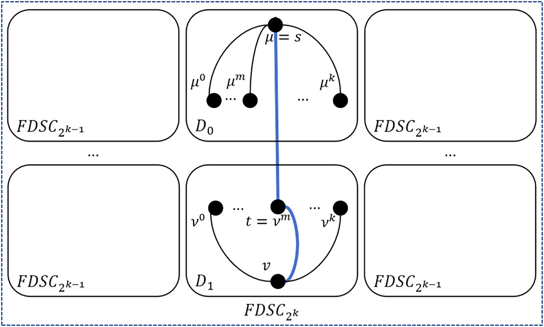
Lemma 4. Let and be any two distinct nodes in the same embeded of , where , and . There exist disjoint paths between and out of .
Proof. By Lemma 2, has an -neighbor and has an -neighbor , which lie in the same embeded of for each with . And we can use algorithm QP to construct a path between and which traverses and for each with . The detailed algorithm is shown as below.
In Algorithm 3, a loop is used to build node disjoint paths between and out of , where and are in a certain embeded .The loop will take iterations. Therefore, it takes time. In lines 2–9, we get the -neighbor of . And in lines 10–17, we get the -neighbor of . In line 18, we use algorithm QP to obtain the path between and which traverses and . In line 20, we return the constructed node disjoint paths between and out of .
| Input: Nodes , , and . |
| Output: d − k disjoint paths in a FDSC2d. |
| 1: for do |
| 2: ; |
| 3: ; |
| 4: ; |
| 5: if then |
| 6: ; |
| 7: else |
| 8: ; |
| 9: end if |
| 10: ; |
| 11: ; |
| 12: ; |
| 13: if then |
| 14: ; |
| 15: else |
| 16: ; |
| 17: end if |
| 18: ; |
| 19: end for |
| 20: return ; |
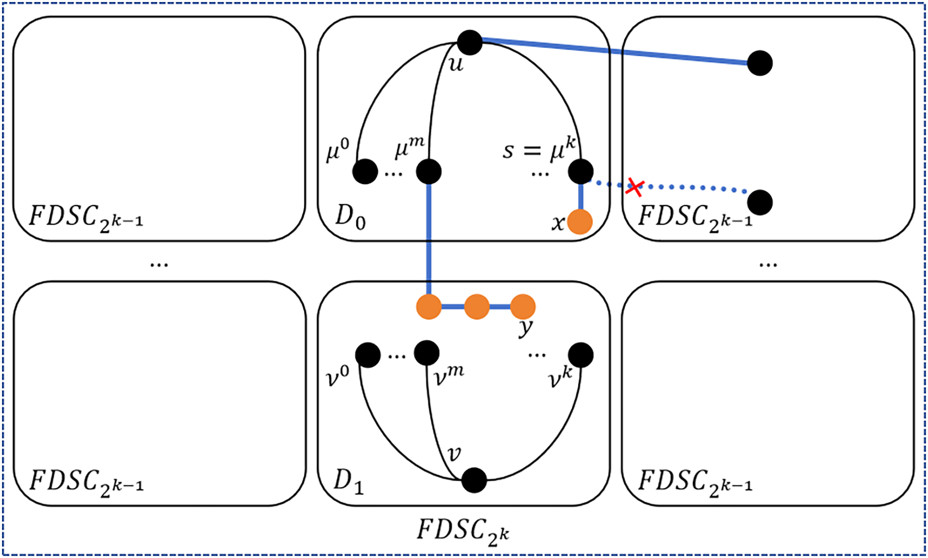
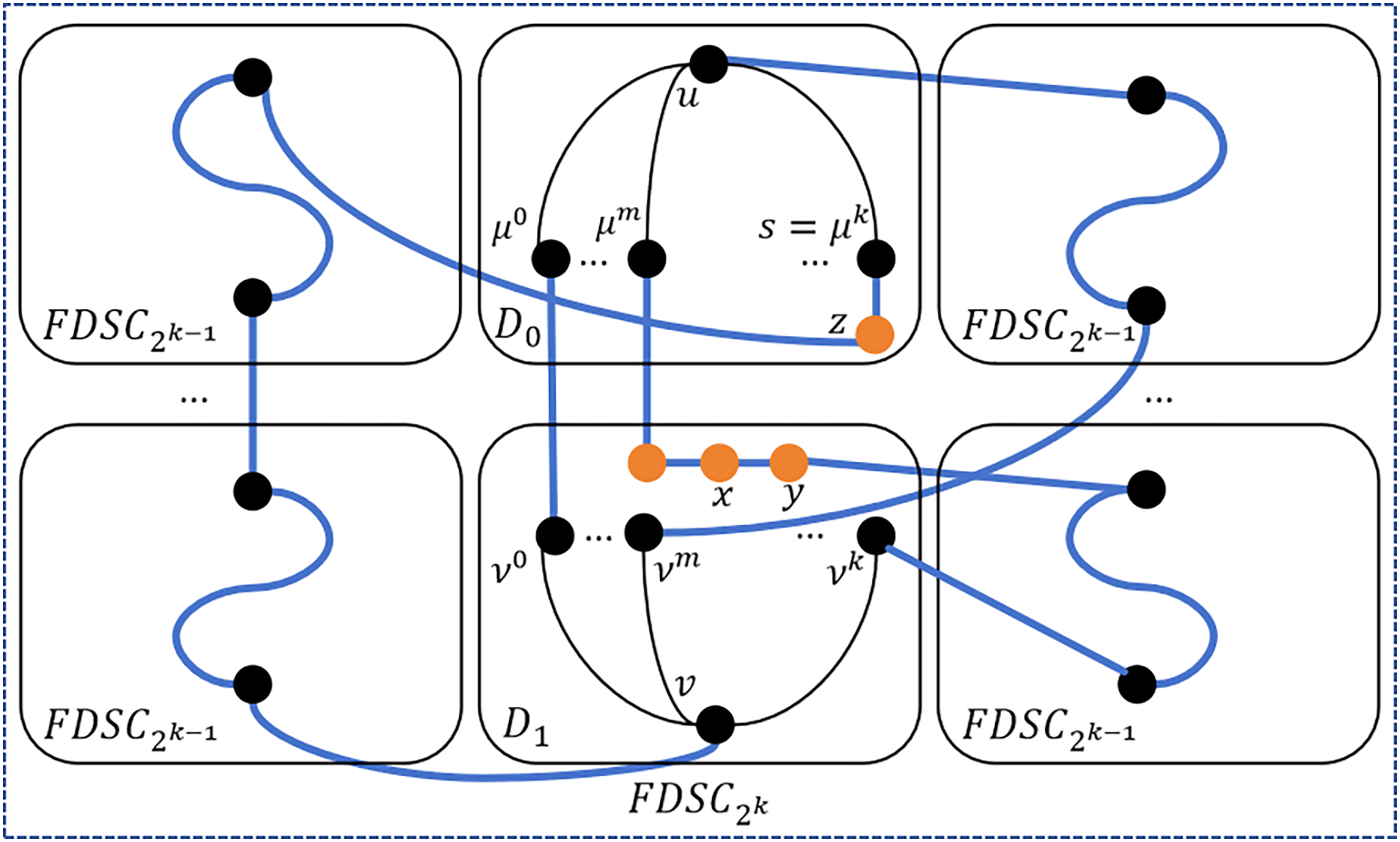
According to Lemma 2, nodes and are in the same embeded , but in the embeded in which and don’t lie. Hence, algorithm QP only occupies the embeded s where and are located and where and don’t lie. By Lemma 2 and Lemma 3, for each with , nodes and are in the same embeded , but in the embeded in which and don’t lie. Hence, algorithm QP only occupies the embeded s where and are located and where and don’t lie. Hence, each path in algorithm DisjointPathOutFDSCK is disjoint. Then, there exist disjoint paths between and out of . Please see Fig. 4 for an illustration.
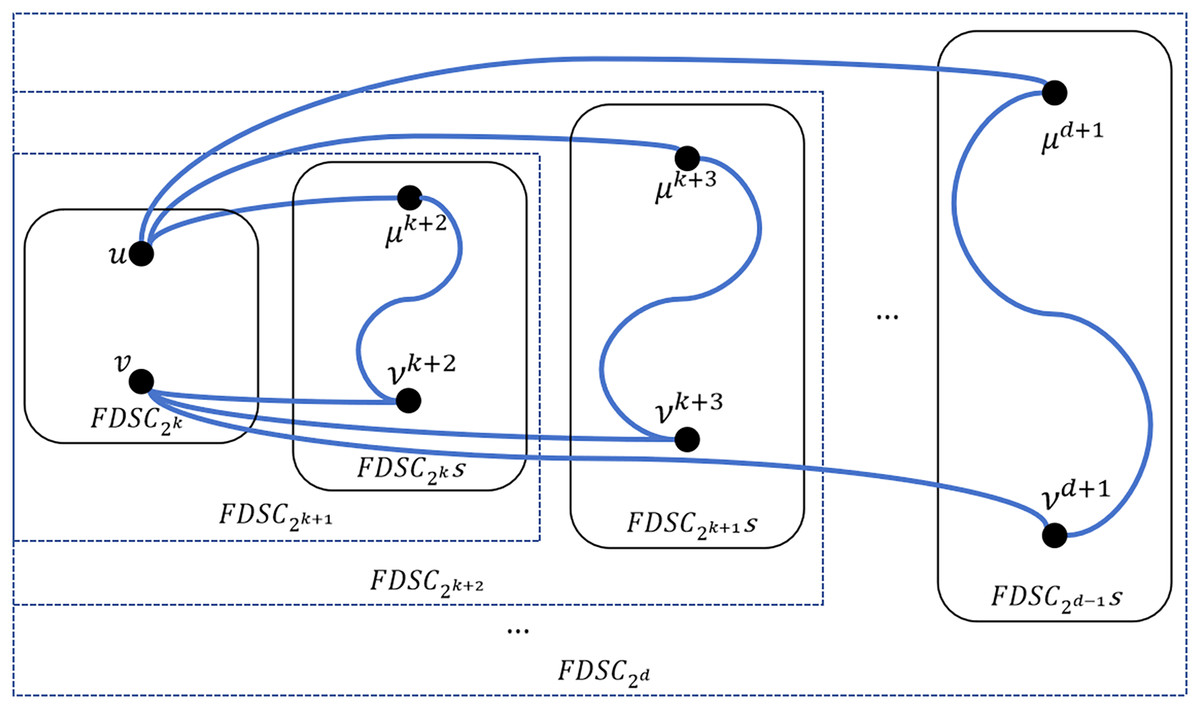
Figure 4: An example of one to one node disjoint paths between and out of .
Each pair of and can lie in different s. In the worst case, is the longest path which occupies two embeded s. Since the diameter of is , then in theory, the maximum length of these paths is .
Lemma 5. Let and be any two distinct nodes in the same embeded of ( and ). There exist node disjoint paths between and in .
Proof. Let and . In this case, , then . Since is a complete graph, we can construct 3 disjoint paths between and with algorithm DisjointPathInFDSC2 ( ) (Algorithm 4).
| Input: Nodes , , and . |
| Output: 3 disjoint paths in an embeded FDSC2. |
| 1: |
| 2: for do |
| 3: ; |
| 4: end for |
| 5: ; |
| 6: return ; |
Then, we use algorithm DisjointPathOutFDSCK to construct disjoint paths out of .
Algorithm 5 is used to build node disjoint paths between and , where , . In line 1, we get three disjoint paths in , which takes time. In line 3, we use algorithm DisjointPathOutFDSCK to obtain disjoint paths between and out of . Since algorithm DisjointPathOutFDSCK takes time, the time complexity of Algorithm 5 is . In line 5, we return the constructed node disjoint paths between and . The theoretical maximum length of is where . If , then Algorithm 5 only needs to construct three disjoint paths in . The theoretical maximum length of these three disjoint paths in is 2. Please see Fig. 5 for an illustration.
| Input: Nodes , and . |
| Output: disjoint paths in . |
| 1: DisjointPathInFDSC2( ); |
| 2: if then |
| 3: DisjointPathOutFDSCK( ); |
| 4: end if |
| 5: return ; |
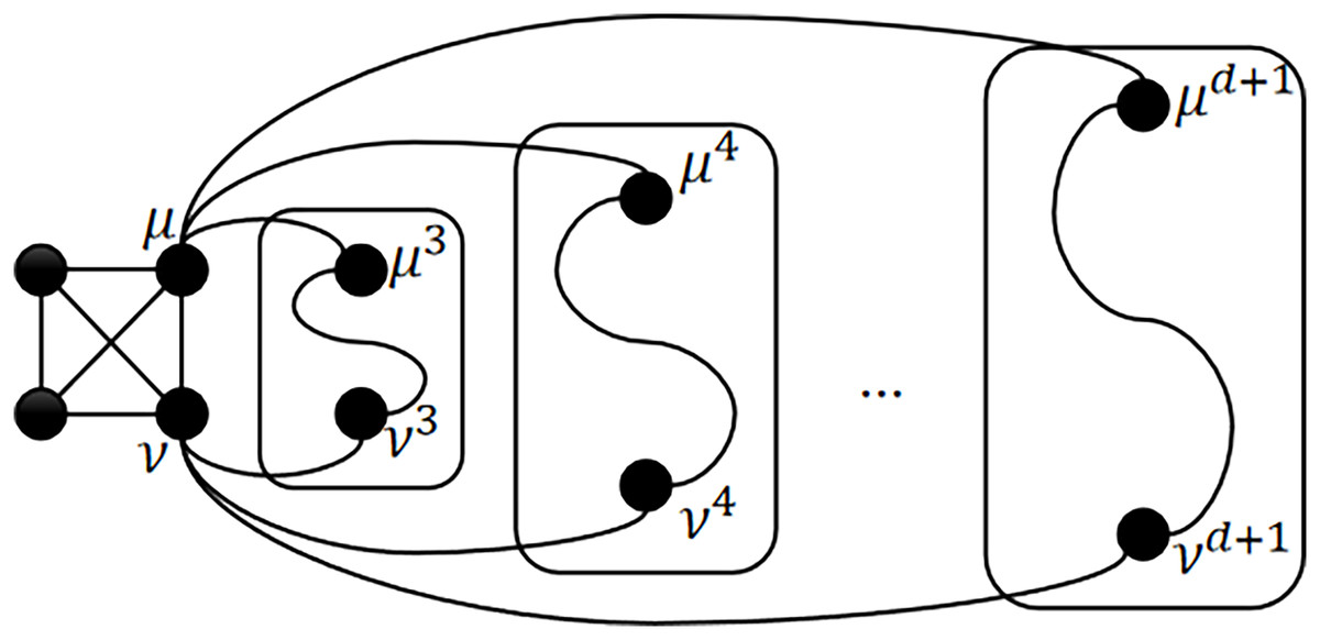
Figure 5: An example of one-to-one node disjoint paths between and in the same .
Lemma 6. Let and be any two distinct nodes in the same embeded of ( and ). There exist node disjoint paths between and in .
Proof. Suppose that and are any two distinct nodes in the same embeded named D. First, we will construct four disjoint paths between and in D. According to the locations of and , we have the following two cases.
Case 1. and are in the same of D.
We can easily get the four disjoint paths with algorithm O2OInFDSC2( ).
Case 2. and are in different s of D.
Suppose that is in and is in , where and are two different s of D. By Property 1(3), each node has three neighbors in . Then, let in and in . We can build four disjoint paths with the following steps.
Step 1: For each in U, if is adjacent with a node in V, build a path as follows. Then remove from U and from V.
(6.1)
Step 2: For each in U, if there is a node such that and are connected to the same , build a path as follows. Then remove from U and from V.
(6.2)
Step 3: For each in U, if there is a node such that and are connected to different s, build a path using the method of Step 2. Then remove from U and from V.
By Property 2, there exist one or two edges between and . Then, we have the following two subcases.
Case 2.1. there exist two edges between and .
In this case, we can construct two disjoint paths between and with Step 1, and two disjoint paths between and with Step 2. Hence, there exist four disjoint paths between and .
Case 2.2. there exists one edge between and .
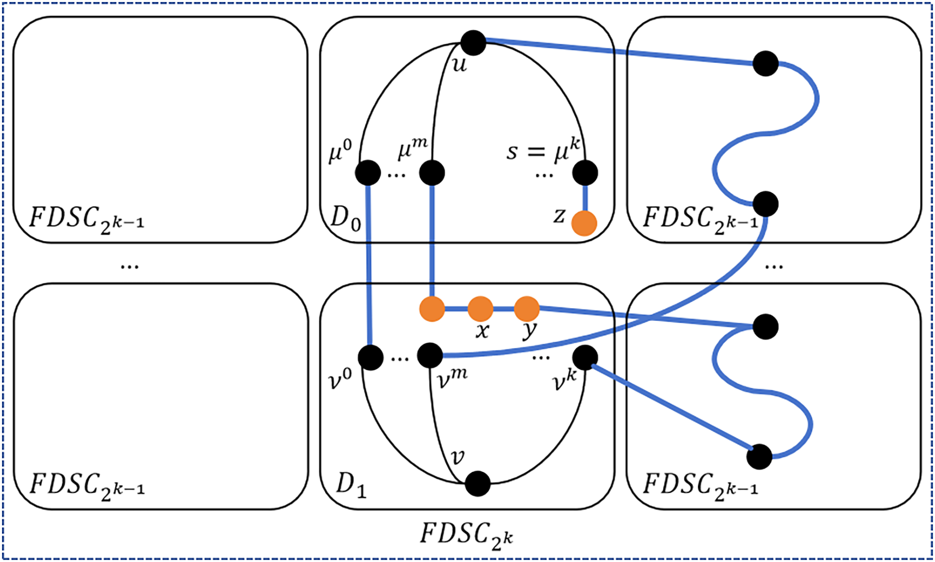
In this case, assume the other two modules of D are named and . With Step 1, we can construct one disjoint path between and . In Step 2, for each pair and where and are in the same , we can construct a disjoint path according to Eq. (6.2) where QP returns . Hence, there exist two disjoint paths between and with Step 2. Let be the subgraph of , containing the nodes not used in Step 2. Since is a complete graph, then is a connected graph. Since the bridge edge between and exists, is connected. Each node in is connected to a different node out of , then and in Step 3 can only connected to , and there exists one disjoint path between and with Step 3. Hence, there exist 4 disjoint paths between and .
For example, in Fig. 2, suppose , and . With Step 1, we can construct a disjoint path , then and . In Step 2, node pairs and are connected to the same , respectively. We can construct two disjoint paths and , then and . We can see that is connected where . In Step 3, is connected to and is connected to . We can build a disjoint path . Hence, there exist 4 disjoint paths between 1000 and 0010.
After building four disjoint paths in the embeded , we can build disjoint paths out of the embeded with algorithm DisjointPathOutFDSCK. Hence, there exist disjoint paths between any two distinct nodes and in .
Algorithm O2OInFDSC4 is used to build node disjoint paths between and , where and are in the same embeded . In lines 1–3, if and are in the same embeded FDSC2, we can get disjoint paths with algorithm O2OInFDSC2. In lines 4–9, we use algorithm DisjointPathInFDSC4 (Algorithm 6) to construct four disjoint paths in the embeded , which takes time. Then use DisjointPathOutFDSCK to obtain disjoint paths between and out of the embeded , which takes time. Therefore, the time complexity of Algorithm 7 is . In line 10, we return the constructed node disjoint paths between and . The theoretical maximum length of is where . If , then Algorithm 7 needs to construct 4 disjoint paths in . The theoretical maximum length of 4 disjoint paths in is 7, and the path is generated in Step 3.
| Input: Nodes , and . |
| Output: 4 disjoint paths between μ and ν in an embeded FDSC4. |
| 1: paths ← []; ; ; |
| 2: for each do Δ Step 1 |
| 3: for each do |
| 4: if isAdjacent(s, t) then |
| 5: build a path P according to Eq. (6.1); |
| 6: paths.append(P); |
| 7: U.remove(s); V.remove(t); |
| 8: end if |
| 9: end for |
| 10: end for |
| 11: for each do Δ Step 2 |
| 12: for each do |
| 13: if s and t are connected to the same FDSC2 then |
| 14: build a path P according to Eq. (6.2); |
| 15: paths.append(P); |
| 16: U.remove(s); V.remove(t); |
| 17: end if |
| 18: end for |
| 19: end for |
| 20: for each do Δ Step 3 |
| 21: for each do |
| 22: if s and t are connected to different FDSC2s then |
| 23: build a path P according to Eq. (6.2); |
| 24: paths.append(P); |
| 25: U.remove(s); V.remove(t); |
| 26: end if |
| 27: end for |
| 28: end for |
| 29: return paths; |
| Input: Nodes , , and . |
| Output: disjoint paths in . |
| 1: if μ and ν are in the same embeded FDSC2 then |
| 2: O2OInFDSC2 ); |
| 3: end if |
| 4: if μ and ν are in different embeded FDSC2s then |
| 5: DisjointPathInFDSC4 ); |
| 6: if then |
| 7: DisjointPathOutFDSCK( ); |
| 8: end if |
| 9: end if |
| 10: return ; |
Lemma 7. Let be any node in the embeded with identifier B in ( , and ) and . Each in U is connected to a different module of .
Proof. Suppose that and are in , and they are connected to the same , where and are two modules of . By Property 2, we have and , or vice versa, where is a -digit binary string. Hence, and are in the same embeded , but in different embeded s of . According to the definition of , . Then and form a triangle. There is no triangles in , and for , an -edge is added for each node in the embeded s. Hence, there only exist trangles in the embeded s in . Then, and should be in the same embeded , which conflicts with that and are in different embeded s. Hence, each in U is connected to a different module of .
Let in and . We can see that each element in U is connected to a different element in in Fig. 3.
Lemma 8. Let and be any two nodes in different embeded s of the same embeded in where , and . There exist node disjoint paths between and in .
Proof. Suppose D is the embeded , and are two embeded s of D where and . By Property 1(2), each node has neighbors in . Let in , , in , and . First, we construct disjoint paths between and in D. Then use algorithm DisjointPathOutFDSCK to obtain the disjoint paths between and out of D. Considering the locations of and in , we have the following steps to construct disjoint paths.
Step 1: Identify the vertex pairs and such that and are directly connected. If such pairs are found, for each pair of and , use the following method to construct a path P between and , and then remove from U and from V. Please see Fig. 6 for an illustration. In this case, is directly connected to , then there exists a path .
(7.1)
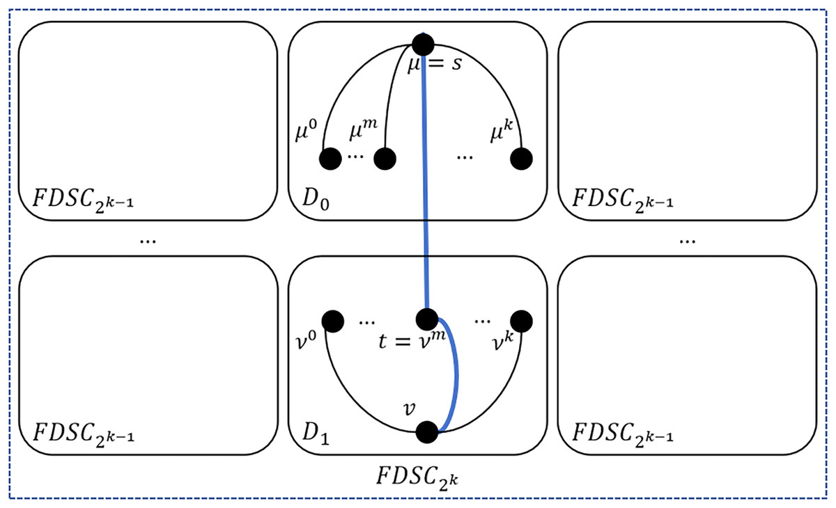
Figure 6: An illustration of step 1.
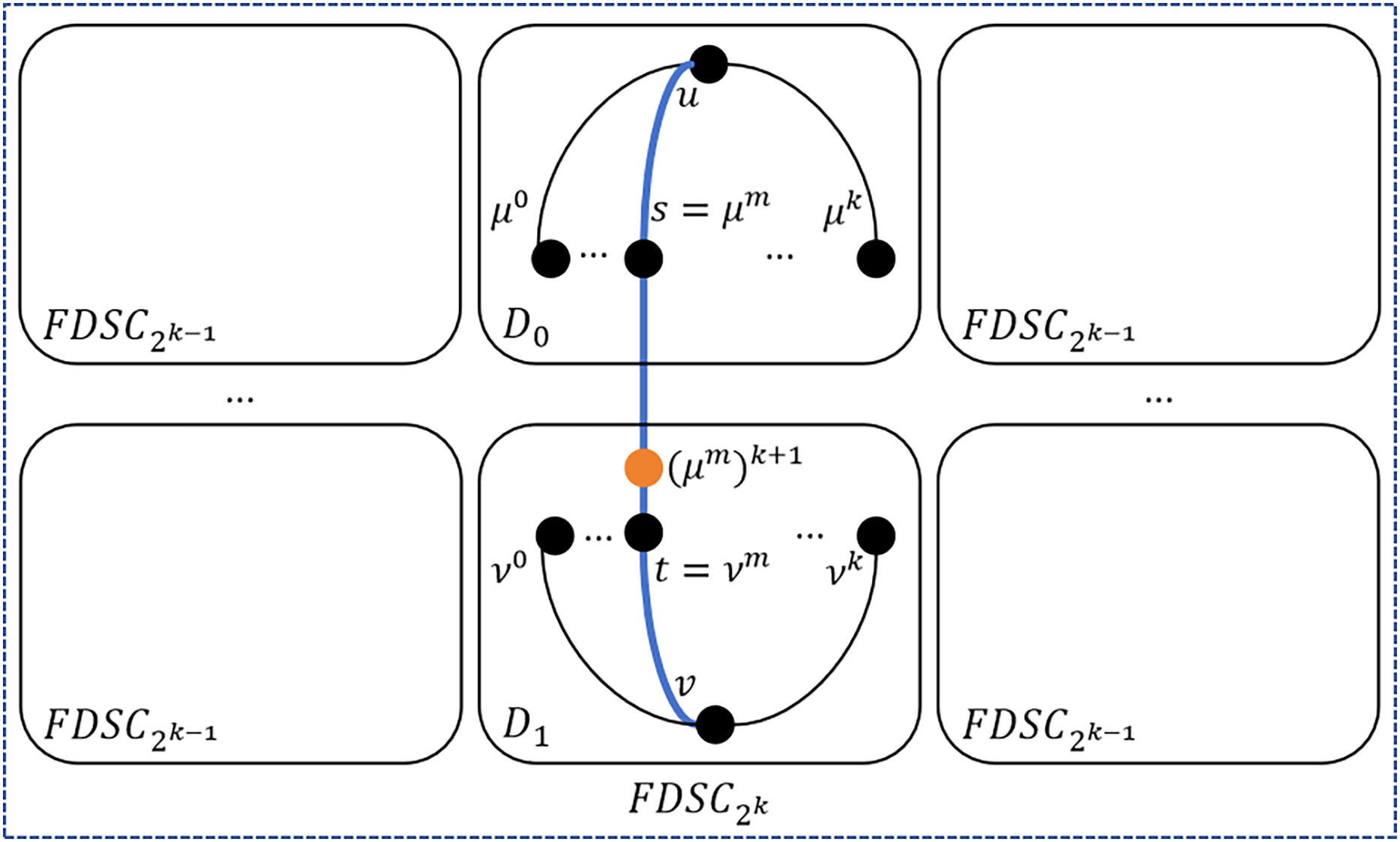
Step 2: Identify the vertex pairs and such that the external neighbor of in is directly connected to . If such pairs are found, for each pair of and , use the following method to construct a path between and , and then remove from U and from V. Please see Fig. 7 for an illustration. In this case, , whose external neighbor is directly connected to , then there exists a path .
(7.2)
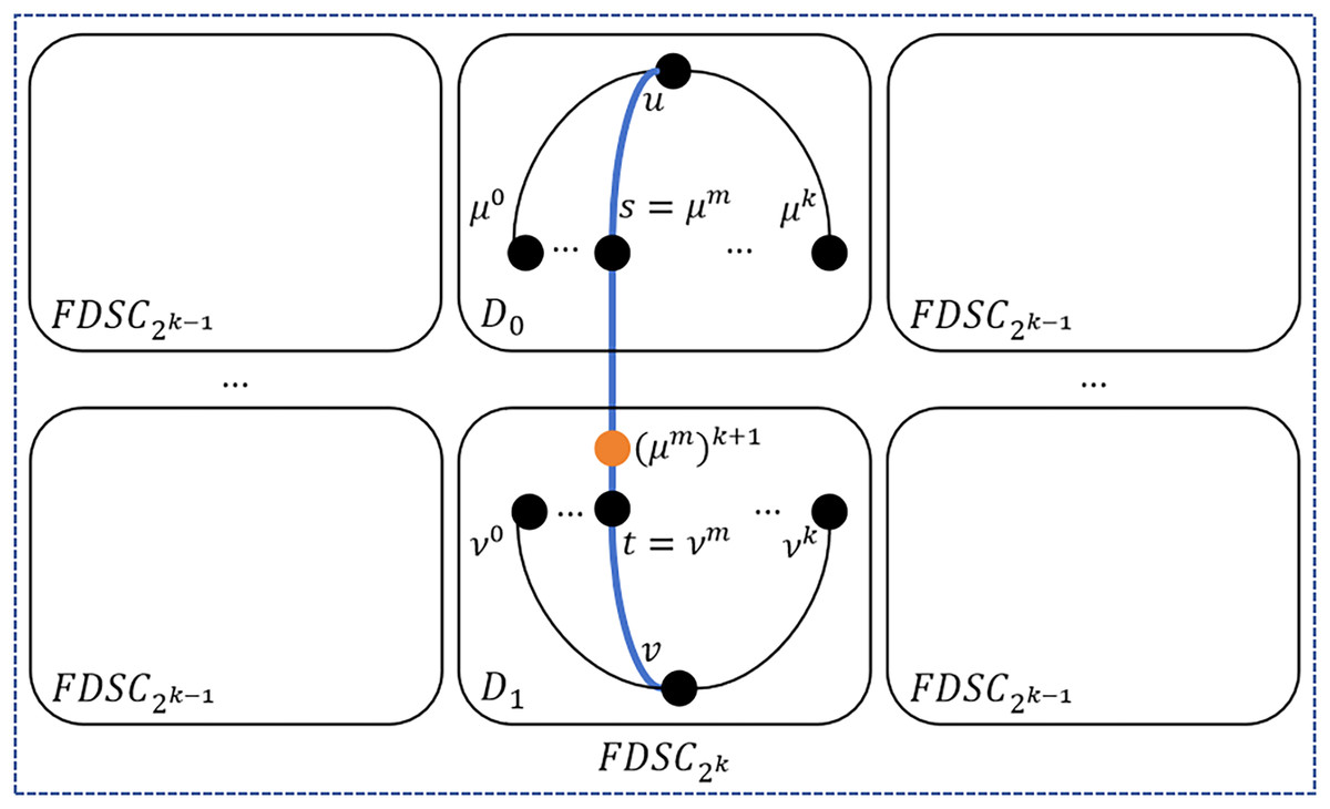
Figure 7: An illustration of step 2.
Step 3: Identify the vertex pairs and such that the external neighbor of in is directly connected to . If such pairs are found, for each pair of and , use the following method to construct a path P between and , and then remove from U and from V. Please see Fig. 8 for an illustration. In this case, , whose external neighbor is directly connected to , then there exists a path .
(7.3)
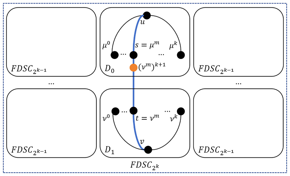
Figure 8: An illustration of step 3.
Step 4: Check each vertex in U. If is connected to and is not adjacent to any of the vertices in V and , we select an edge such that , and . Then put into U to replace , and build a partial path from to as follows. Since and by Lemma 7, then for the worst case. Hence, we can easily find a node such that and . Please see Fig. 9 for an illustration. In this case, , then there exists a partial path .
(7.4)

Figure 9: An illustration of step 4.
Step 5: Check each vertex in V. If is connected to and is not adjacent to any of the vertices in U and , then similiar to Step 4, select an edge such that , and . Then put into V to replace , and build a partial path from to as follows. Please see Fig. 10 for an illustration. In this case, , then there exists a partial path .
(7.5)
Figure 10: An illustration of step 5.
Step 6: If , check each vertex in . For each , if and are connected to the same module in D, select a neighbor of in such that . Then, put into U to replace and construct a partial path from to as follows. By Lemma 7, any two different neighbors of in are connected to different modules in D. Then only and one of its neighbor in can be linked to the same module. Since and each neighbor of is connected to a different module, we can easily find a neighbor of such that . Please see Fig. 11 for an illustration. In this case, , then there exists a partial path .
(7.6)
Figure 11: An illustration of step 6.
Step 7: If , check each vertex in . Similar to Step 6, for each , if and are connected to the same module in D, then select a neighbor of in such that . Put into V to replace and construct a partial path from to according to Eq. (7.6).
Step 8: Identify vertex pairs and , such that and are connected to the same . If found, for each pair of and , place into set , into set , and then remove from U and from V.
Step 9: For each pair of vertices and which are connected to the same , use the following method to construct a disjoint path between and . If is the replaced node generated in step 4 or step 6, then set S as the partial path generated in step 4 or step 6. Otherwise, set S to an empty string. If is the replaced node generated in step 5 or step 7, then set T as the partial path generated in step 5 or step 7. Otherwise, set T to an empty string. Afterwards, construct a path P between and with algorithm QP, and connect P with S and T. Then, we can build a disjoint path between and . Please see Fig. 12 for an illustration.
(7.7)
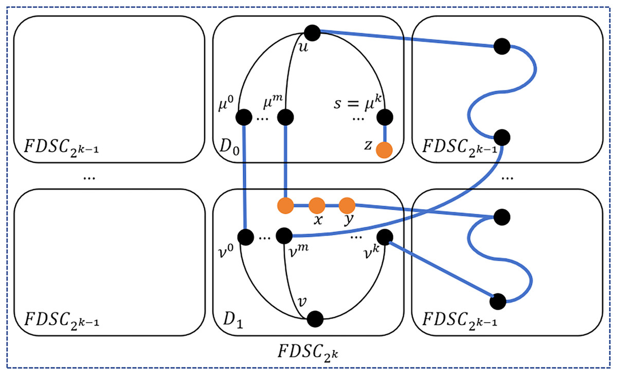
Figure 12: An illustration of step 9.
We give the detailed algorithm as follows.
Step 10: For each pair of vertices and which are connected to the different s, use a method similar to Step 9 to construct a disjoint path between and . Please see Fig. 13 for an illustration.
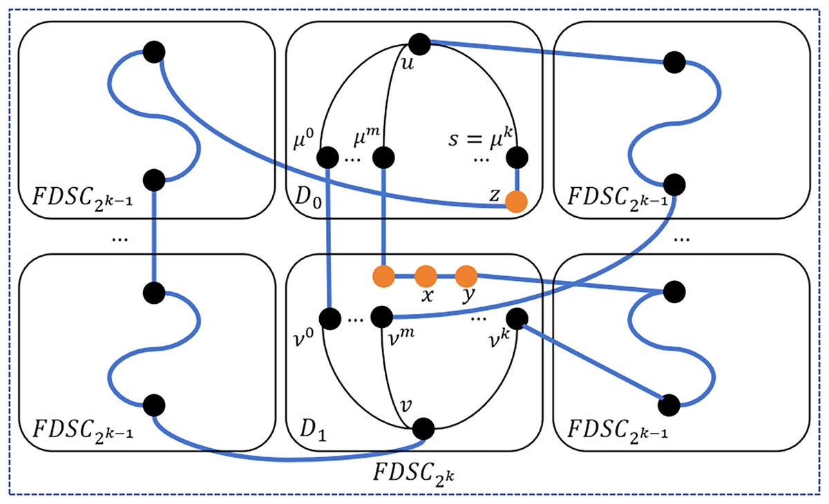
Figure 13: An illustration of step 10.
Step 11: If , then has a neighbor in and has a neighbor in for each with . We can build disjoint paths between and with algorithm DisjointPathOutFDSCK.
In lines 3–6, construct a path for each and , if . In lines 7–16, construct a path for each and , if or . In lines 17–23, check each vertex s in U, if , select an edge such that , and . In lines 24–30, check each vertex t in V, if , select an edge such that , and . In lines 31–39, if and are connected to the same module of D, then select a neighbor of in such that . In lines 40–48, if and are connected to the same module of D, then select a neighbor of in such that . In lines 49–52, put and connected to the same module of D into and , respectively. In lines 53–56, construct a path for each and connected to the same module of D between and with Algorithm 8. In lines 57–60, construct a path for each and connected to different modules of D between and with Algorithm 8. In lines 61–63, construct disjoint paths out of D between and .
| Input: Nodes and t in . |
| Output: a disjoint path between μ and ν in . |
| 1: S ← “”; T ← “”; |
| 2: if s was generated in step 4 or step 6 then |
| 3: S ← partial path from step 4 or 6; |
| 4: end if |
| 5: if t was generated in step 5 or step 7 then |
| 6: T ← partial path from step 5 or 7; |
| 7: end if |
| 8: construct a path P according to Eq. (7.7); |
| 9: return P; |
From Step 1 to Step 3, for each vertex pair and which are adjacent or connected with a common neighbor, we construct a disjoint path between and which traverses and . Each step takes time. From Step 4 to Step 7, we ensure that the vertices in U and V are connected to different modules of , respectively. Each step takes iterations. From Step 8 to Step 10, we first construct disjoint paths between and which traverses vertex pairs connected to the same module of D, then we construct disjoint paths between and which traverses vertex pairs connected to different modules of D. Each step has less than or equal to iterations. Hence, the time complexity from Step 1 to Step 10 is . In Step 11, we construct disjoint paths between and out of D. Since the time complexity of algorithm DisjointPathOutFDSCK is , the time complexity of algorithm O2OInFDSCK is . When approaches , dominates the time complexity of algorithm O2OInFDSCK. Hence, is the time complexity of algorithm O2OInFDSCK in the worst case.
Since and , then we can build disjoint paths between and in from Step 1 to Step 10. In Step 11, we can build disjoint paths between and out of . Hence, there exist node disjoint paths between and in .
In the worst case, is the replaced node in Step 4 and is the replaced node in Step 5, where and are connected to different modules of . Set S as the partial path generated in Step 4 where and set T as the partial path generated in Step 5 where . Then, and the theoretical maximum path length is for .
Theorem 1. Let and be any two distinct nodes in the same embeded of where , and . There exist node disjoint paths between and in .
Proof. We have the following three cases.
Case 1. and are in the same embeded .
By Lemma 5, the theorem holds in this case.
Case 2. and are in the same embeded .
By Lemma 6, the theorem holds in this case.
Case 3. and are in the same embeded where .
By Lemma 8, the theorem holds in this case.
Hence, there exist node disjoint paths between and in where and are any two distinct nodes in the embeded with .
Based on Algorithms 5, 7 and 9, we define the main algorithm to construct disjoint paths between and . Algorithm 10 is an implementation of Theorem 1. Since the theoretical maximum path lengths for Algorithms 5, 7 and 9 is and , Hence, the theoretical maximum path length for Algorithm 10 is for . For , the theoretical maximum path length for Algorithm 10 is 2, and for , the theoretical maximum path length for Algorithm 10 is 7. The time complexity of algorithms O2OInFDSC2, O2OInFDSC4 and O2OInFDSCK are , and , respectively. Therefore, is the time complexity of algorithm O2OMain.
| Input: Nodes , , and . |
| Output: disjoint paths between μ and ν in . |
| 1: paths ← []; ; ; |
| 2: for each and where doΔ Step 1 |
| 3: construct a path P according to Eq. (7.1); |
| 4: paths.append(P); |
| 5: U.remove(s); V.remove(t); |
| 6: end for |
| 7: for each and where do Δ Step 2 |
| 8: construct a path P according to Eq. (7.2); |
| 9: paths.append(P); |
| 10: U.remove(s); V.remove(t); |
| 11: end for |
| 12: for each and where do Δ Step 3 |
| 13: construct a path P according to Eq. (7.3); |
| 14: paths.append(P); |
| 15: U.remove(s); V.remove(t); |
| 16: end for |
| 17: for each do Δ Step 4 |
| 18: if and and then |
| 19: select an edge such that , and . |
| 20: U.replace(y, s); |
| 21: build a partial path from s to y according to Eq. (7.4); |
| 22: end if |
| 23: end for |
| 24: for each do Δ Step 5 |
| 25: if and and then |
| 26: select an edge such that , and . |
| 27: V.replace(y, t); |
| 28: build a partial path from t to y according to Eq. (7.5); |
| 29: end if |
| 30: end for |
| 31: if then Δ Step 6 |
| 32: for each do |
| 33: if s and μ are connected to the same module in D then |
| 34: select a neighbor z of s in D0 such that . |
| 35: U.replace(z, s); |
| 36: build a partial path from μ to z according to Eq. (7.6); |
| 37: end if |
| 38: end for |
| 39: end if |
| 40: if thenΔ Step 7 |
| 41: for each do |
| 42: if s and ν are connected to the same module in D then |
| 43: select a neighbor z of s in D1 such that . |
| 44: V.replace(z, s); |
| 45: build a partial path from ν to z according to Eq. (7.6); |
| 46: end if |
| 47: end for |
| 48: end if |
| 49: for each and connected to the same module of D do Δ Step 8 |
| 50: U1.add(s); V1.add(t); |
| 51: U.remove(s); V.remove(t); |
| 52: end for |
| 53: for each and connected to the same module of D do Δ Step 9 |
| 54: DisjointPathInFDSCK ; |
| 55: paths.append(P); |
| 56: end for |
| 57: for each and connected to different modules of D do Δ Step 10 |
| 58: DisjointPathInFDSCK ; |
| 59: paths.append(P); |
| 60: end for |
| 61: if then Δ Step 11 |
| 62: paths.append(DisjointPathOutFDSCK( )); |
| 63: end if |
| 64: return paths; |
| Input: Nodes , , and . |
| Output: node disjoint paths in FDSCn. |
| 1: ; |
| 2: if then |
| 3: return O2OInFDSC2( ); |
| 4: else if then |
| 5: return O2OInFDSC4( ); |
| 6: else |
| 7: return O2OInFDSCK( ); |
| 8: end if |
Table 3 compares the number of generated paths, longest path length, time complexity of the disjoint path algorithms for and some other hypercube variants. has a smaller time complexity because grows far more slowly than . For large , this makes ’s disjoint path algorithm much more efficient than those of other hypercube variants. For the longest path length, has a length of , which is longer than that of twisted cubes ( ) and folded hypercubes ( ) but comparable to hypercubes ( ) and better than crossed cubes and m bius cubes( ).
| Network | Diameter | Number of generated paths | Longest path length | Time complexity |
|---|---|---|---|---|
| Hypercubes | ||||
| Crossed cubes | ||||
| Twisted cubes | ||||
| Folded hypercubes | ||||
| M bius cube | or | |||
Performance evaluation
In the section, we conduct a computer experiment to inspect the practical performance of the algorithm O2OMain. We implemented the algorithm using Java programming language, and the target machine is equipped with an Intel Core i5-7200U CPU 2.80 GHz and 12 GB RAM. For with various values of , we constructed node disjoint paths between any two distinct nodes for a certain number of times. Then we evaluated the average path length and the average of the maximum path lengths for each . Taking into account the impact of both the parameter and the positions of the two nodes in when constructing disjoint paths, we randomly selected six distinct node pairs for , 120 distinct node pairs for and 10,000 distinct node pairs for , respectively.
For each value of , Fig. 14 illustrates the average of maximum and the average lengths of all disjoint paths obtained using algorithm O2OMain compared with theoretical maximum lengths. The theoretical maximum lengths take values of , 7, , corresponding to , , ( ). We can see that the actual average of maximum lengths are very close to the theoretical maximum lengths when . However, when , the gap between them gradually becomes larger.
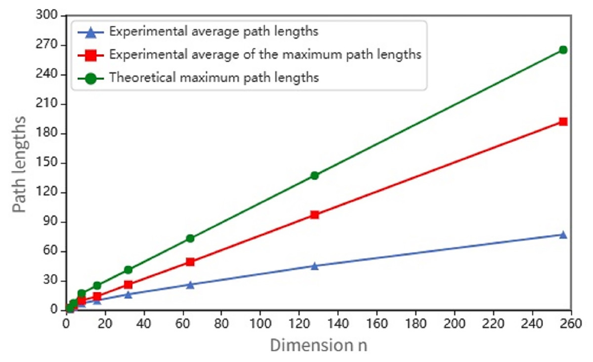
Figure 14: Results of average of maximum and average path lengths compared with the theoretical maximum path lengths.
Conclusion
As a newly proposed hypercube variant, has many superior properties over the hypercube. In this work, we investigate the disjoint path problem for . The main contributions of this work are that we give an algorithm QP to build a path between any two distinct nodes and , as well as an algorithm O2OMain for constructing one-to-one disjoint paths in . In future work, we can consider the construction of node-to-set disjoint paths (Wang et al., 2022; Kocik, Hirai & Kaneko, 2016; Ling & Chen, 2014) or set-to-set disjoint paths (Zhuang et al., 2024) for . In addition, component diagnosticability (Liu et al., 2022) and extra fault diagnosticability (Lin et al., 2021) are also future research directions.