
Trajectory planning for uncrewed combat aircraft penetration with dynamic radar cross section constraint
- Published
- Accepted
- Received
- Academic Editor
- Giovanni Angiulli
- Subject Areas
- Algorithms and Analysis of Algorithms, Artificial Intelligence, Data Mining and Machine Learning, Emerging Technologies, Neural Networks
- Keywords
- Dynamic RCS, UCAV, Trajectory planning, Penetration mission
- Copyright
- © 2025 Wang et al.
- Licence
- This is an open access article distributed under the terms of the Creative Commons Attribution License, which permits using, remixing, and building upon the work non-commercially, as long as it is properly attributed. For attribution, the original author(s), title, publication source (PeerJ Computer Science) and either DOI or URL of the article must be cited.
- Cite this article
- 2025. Trajectory planning for uncrewed combat aircraft penetration with dynamic radar cross section constraint. PeerJ Computer Science 11:e3444 https://doi.org/10.7717/peerj-cs.3444
Abstract
The survivability and mission effectiveness of uncrewed combat aircraft (UCAV) is directly dependent on the probability of detection as determined by radar cross section (RCS) characteristics. This article presents a trajectory optimization method incorporating dynamic RCS constraints, addressing the limitation of existing approaches that model radar threats as static regions, thereby improving the adaptability of UCAVs to complex battlefield penetration scenarios. It develops a dynamic RCS model to calculate the detection probability, thereby overcoming the limitation of existing radar threat models that rely solely on distance or static RCS interpolation table. Furthermore, an improved black-winged kite algorithm incorporating dynamic selection scoring mechanism, random cross-up update strategy is presented. The proposed method combines multi-structural optimization to modify the position update strategy for hovering predation. Simulation results validate that the algorithm efficiently determines optimal trajectories under dynamic RCS constraints in multi-objective environments, ensuring rapid and accurate path planning for UCAV penetration.
Introduction
The increasing role of uncrewed combat aircraft (UCAV) in modern warfare, while driving the development of advanced countermeasures, has resulted in a rapidly evolving and highly adversarial air warfare environment (Li et al., 2022a, 2022b; Kuhnert et al., 2024). Specifically, UCAV penetration missions face unprecedented challenges due to the proliferation of integrated air defense systems, multi-domain sensor networks, and dynamic threat areas (Ge, Xiang & Li, 2024; Yang et al., 2024). In order to maintain mission effectiveness, UCAVs must be equipped with adaptive trajectory planning capabilities to navigate complex electromagnetic interference environments while minimizing detection probability and maximizing penetration success under time-critical constraints (Xu et al., 2020; Zhong, Xiao & Gao, 2025).
The purpose of UCAV penetration trajectory planning is to ultimately maximize the probability of survival by optimizing and making real-time decisions to follow the most appropriate path to a specific endpoint in an adversarial environment (Zhang et al., 2020a; Liu et al., 2021; Luo, Liang & Li, 2023; Zhang et al., 2025b). Trajectory planning for UCAVs is often formulated as a constrained optimization problem that integrates dynamic operational constraints such as threat area avoidance, fixed cruise altitude, and mission objectives, among other requirements (Liu et al., 2023). For UCAVs to compete for air power in high-risk environments, they must have the means and capabilities to break out of complex radar environments. UCAVs face mainly different types of radar detection threats in their missions, and the probability of being detected by radar is closely related to the radar cross section (RCS) (Ezuma et al., 2022; Costley et al., 2022; Taj et al., 2023). The attitude of UCAV under different flight paths affects its RCS (Persson & Bull, 2016). Therefore, it is critical to use RCS to develop a trajectory that minimizes the likelihood of radar detection.
Common constraints in UCAV flight trajectory planning studies include obstacle threat minimization, radar threat minimization, path constraints, flight altitude constraints, and flight angle constraints (Liu et al., 2021, 2023; Luo, Liang & Li, 2023; Gao et al., 2024). The main focus in current research for minimization of radar threat constraint is to model the radar threat as a static hazardous area and assess the risk of collision utilizing the Euclidean distance separating UCAVs from the threat source. An A* algorithm that considers static 3DRCS values is used for trajectory planning and no longer uses a simple radar model to estimate risk exposure (Guan et al., 2024). Traditional trajectory planning methods ignore the dynamic changes in RCS caused by the fuselage attitude angle and radar line-of-sight angle, resulting in the existing models being unable to deal with the time-varying RCS constraints in complex battlefield scenarios. A method is proposed to calculate the RCS constraints in trajectory planning using the physical optics method (Woo, Shin & Kim, 2019). However, the reference trajectory obtained by this method is rather coarse. A penetration path planning algorithm for stealthy UAVs considering dynamic RCS is proposed to address the challenge of complex environments containing Bogie or Bandit threats (Zhang et al., 2020b). However, this model treats the 3DRCS as a single ellipsoid, which still has a gap with reality. Zhang et al. (2023) proposes a combined approach integrating the minimum radar cross-section tactic with an enhanced A* algorithm. By accounting for sudden appearances of rogue radar systems and moving targets, it enables stealth UAVs to achieve efficient, optimized online penetration path planning in complex dynamic environments, effectively reducing the probability of radar detection. However, since radar cross-section tactics are applied only as reactive measures rather than being integrated as core optimization objectives from the outset, their rule-driven hierarchical structure inherently limits the ability to achieve globally optimal solutions. In complex operational environments, it is clear that current trajectory planning research modeling for dynamic RCS constraints cannot meet the requirements of surprise defense.
In addition to this, algorithms applied to trajectory planning are developing rapidly. Traditional algorithms often face problems such as computational redundancy, issues such as suboptimal real-time responsiveness, and a tendency to become trapped in local optima often arise due to their reliance on global information and fixed rules. Heuristic algorithms have become an important tool for solving multi-constraint optimization problems in trajectory planning by virtue of their efficient search strategies and dynamic environment adaptability, which significantly enhance the practicality of planning. An improved A* algorithm for path planning of stealth drones infiltrating three-dimensional networked radar environments is proposed by significantly enhancing the search strategy and cost function of the A* algorithm, and closely integrating the dynamic RCS characteristics of stealth drones with the detection model of networked radars (Zhang et al., 2022). To cope with complex optimization problems in agricultural production and biological control, the researchers proposed an improved gray wolf optimization algorithm (NAS-GWO) that incorporates a multi-agency synergy mechanism (Liu et al., 2023). A fusion optimization algorithm of Gray Wolf Optimizer (GWO) and Dubins Path Theory is proposed to address the core requirements of UCAV path planning and precision strikes (Huang et al., 2022). An Intelligent Path Planning Framework Incorporating Immune Plasma Optimization Algorithm (IPA) is proposed (Aslan, 2022). A novel Event-Triggered Multimodal Adaptive Pigeon-Inspired Optimization (ET-MAPIO) algorithm is proposed, to solve the real-time cooperative path planning problem for multiple autonomous UAVs in complex dynamic environments (Zhang et al., 2025c). Furthermore, other intelligent optimization algorithms can be applied to the trajectory planning study, such as the Crow Search Algorithm (CSA) (Abualigah et al., 2024), Teaching-Learning-Based Optimization (TOC) (Ma, Li & Yong, 2024), Grasshopper Optimization Algorithm (GOA) (Alirezapour, Mansouri & Mohammad Hasani Zade, 2024), Puma Optimizar Algorithm (POA) (Abdollahzadeh et al., 2024), Black-winged Kite algorithm (BKA) (Wang et al., 2024), etc. BKA innovatively integrates the dual-mode search mechanism of high-altitude wide area scanning and low-altitude precision predation to realize the rapid localization of global optimal solutions for complex objective functions (Zhang, Wang & Yue, 2024b; Li et al., 2025). However, when faced with complex constraints such as the superposition of multiple threat sources, the algorithm is prone to fall into the local optimization trap due to the lack of an adaptive strategy adjustment mechanism, leading to a decrease in search accuracy and insufficient response speed (Zhang et al., 2025a).
For existing theories, there are still some obvious limitations: Most current trajectory planning studies consider the radar threat as a fixed threat area and only consider the distance between the UCAV and the threat sources, which does not take into account the specific impact on the UCAV, leading to inaccurate threat assessments during penetration maneuvers. Constraints on the RCS are usually static data tables or reduced to invariant ellipsoid models, which are still far from reality. The BKA is slow to find optimal paths under complex constraints and easily falls into local optimality.
This study proposes a penetration planning method for UCAVs that incorporates dynamic RCS constraint. The dynamic RCS is added to the path constraints to take into account changes in the attitude angle and the radar line-of-sight angle relative to the aircraft that occur at all times during the flight of the UCAVs. In the trajectory planning process, the scoring mechanism and the cross-exploration mechanism are fused into BKA to reduce the sensitivity to parameters. This is the core rule of the improved BKA for adaptive decision-making and faster convergence of the algorithm. In addition, the method integrates a multistructure strategy and modifies the cyclic predation update strategy in the traditional BKA algorithm.
This article proceeds with the following structural arrangement. “Problem Formulation” presents the formulation of the problem, including the established UCAV model, the dynamic RCS model, and the assessment of radar threats. The design of the trajectory planning is shown in “Trajectory Planning of UCAV”. In “Improved BKA”, the potential optimized multistructured integrated BKA, named PO-MIBKA, is proposed to rapidly perform the UCAV penetration mission. “Simulation and Experiments” presents the simulation results for different scenarios. Finally, conclusions are given in “Conclusion”.
Problem formulation
In this section, we first present the model of UCAV, followed by the design of dynamic RCS and the radar threat assessment scheme. Finally, we introduce the framework for UCAV penetration trajectory planning.
Kinematic model of UCAV
The kinematic model of the mass based on the inertial coordinate system can be described as:
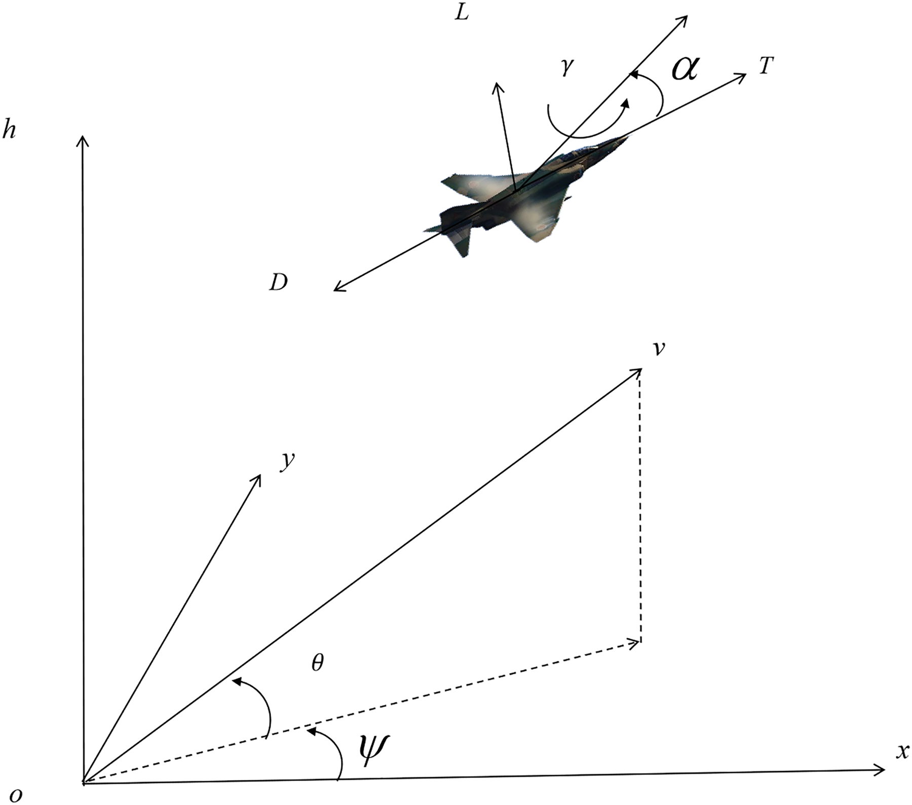
(1) where are the coordinates of the position at time , is the speed of the UCAV. is the track inclination, which is the angle between the velocity and the horizontal plane; is the yaw angle, which is the angle between the projection of the velocity in the horizontal plane and the horizontal axis.
The simplified three-degree-of-freedom model of the UCAV can be expressed as:
(2) where is the acceleration of gravity, is the roll angle, is the angle of attack, is the weight of the UCAV, F is the engine thrust, D is the aerodynamic drag, and L is the aerodynamic lift.
Describing the dynamic behavior of UCAVs during real-time trajectory planning based on the three-degree-of-freedom (3DOF) prime assumption:
(3)
The 3DOF model and the angle relationships are shown in Fig. 1. The drag and lift of the UCAV during flight is modeled as follows:
(4) where is the air density, S is the equivalent cross-sectional area, is the aerodynamic lift coefficient, and is the aerodynamic drag coefficient.
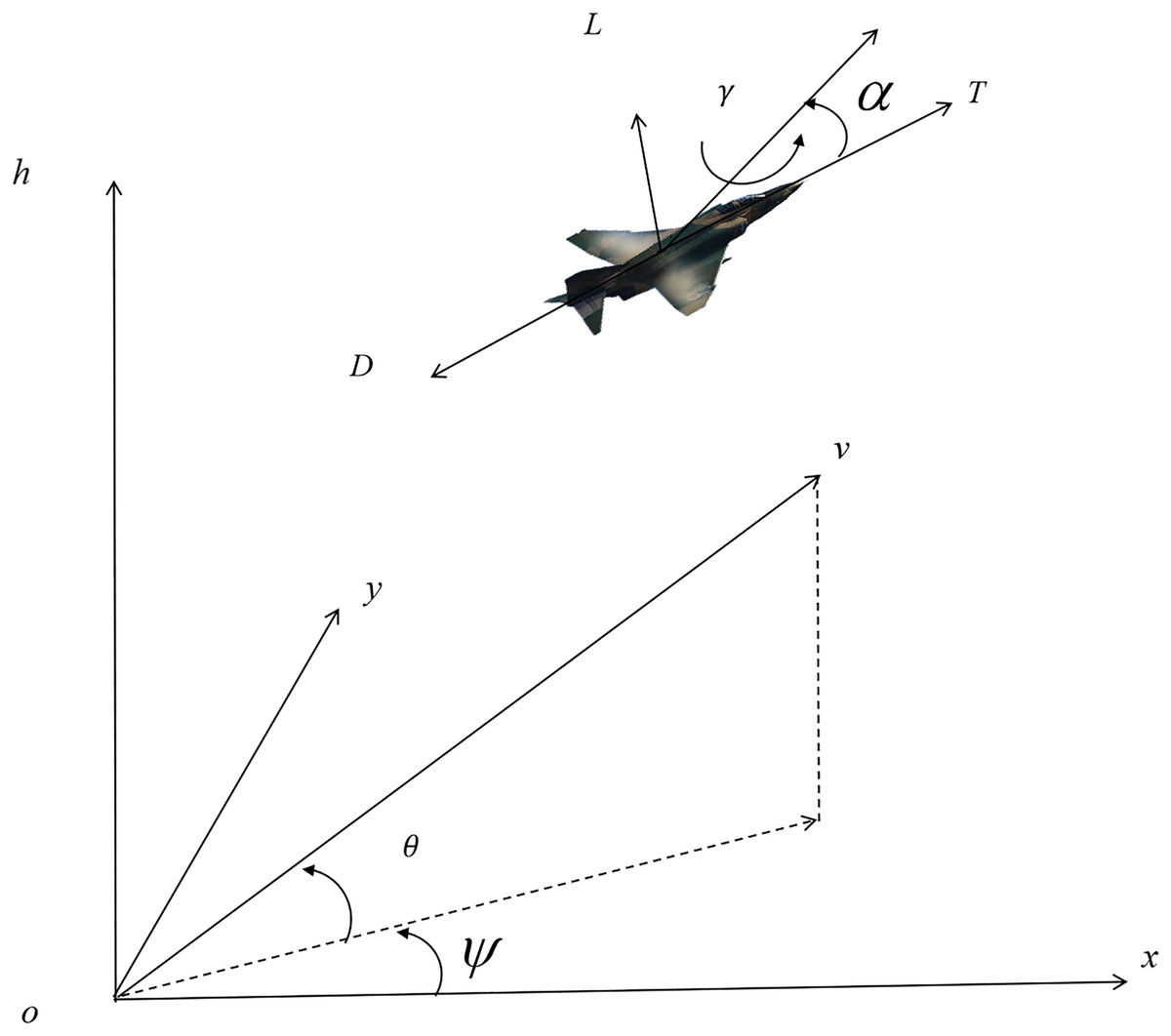
Figure 1: The 3DOF model and the angle relationships.
Remark 1: The following assumptions are made when establishing 3DOF for the UCAV: The UCAV is a rigid body, with no elastic deformation in the process of movement; the additional effects of the Earth’s rotation, revolution and curvature of the Earth are not taken into account; the tactics used are low-altitude surprise defense, with a relatively small range of change in flight altitude, and the acceleration of gravity and the density of the air are constant within the UAV’s flight altitude; that is to say, the mass of the UCAV is constant in the process of flight.
Dynamic RCS model
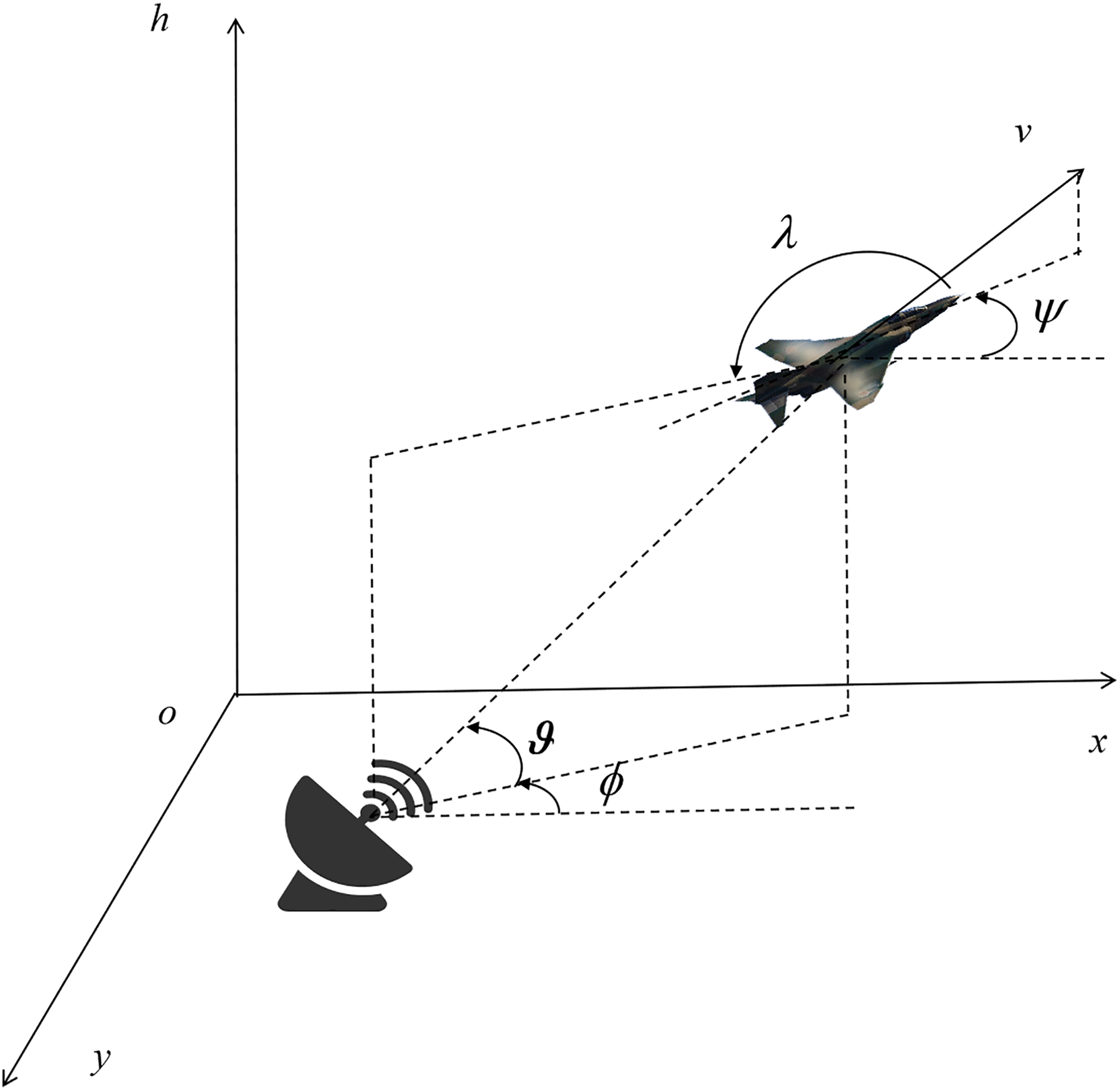
The RCS exhibits a direct positive relationship with its detectability by radar: a larger RCS corresponds to a stronger reflected signal captured by the radar, thereby enhancing the likelihood of target detection and recognition. When analyzing radar threats, the relative attitude and position of the UCAV and the radar need to be modeled to evaluate the RCS value (See Fig. 2; Hu et al., 2022).
(5) where is the position of the radar, is the height angle between the enemy radar and the UCAV, and is the azimuth angle between them.
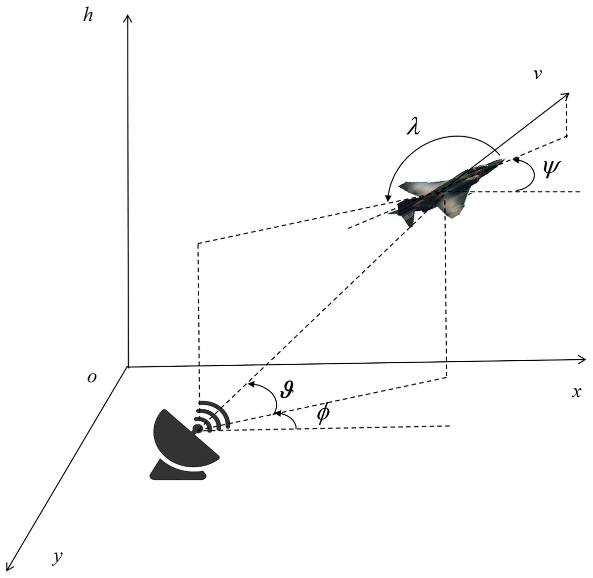
Figure 2: UCAV and radar position attitude relationships.
The RCS of an UCAV exhibits dynamic variations throughout its flight, as the real-time angle between the fuselage and the incident radar wave continuously shifts. Its directional scattering behaviors can be categorized into forward, tail, and vertical scattering patterns: Forward Scattering: When radar waves approach directly from the front of the fuselage, the UCAV demonstrates relatively low RCS values due to the alignment that minimizes wave reflection. Tail Scattering: A significant increase in RCS is observed when radar waves impinge from the rear direction, as the structural geometry at the tail section tends to enhance electromagnetic wave reflection. Vertical Scattering: Incidence of radar waves from the top or bottom of the fuselage results in comparatively higher RCS magnitudes, primarily influenced by the vertical surface configurations that offer larger effective reflection areas. The relationship between dynamic RCS and UCAV attitude is designed accordingly:
(6) where , and and are process variables.
(7)
The model will be used as one of the constraints.
Radar threat assessment
After the UCAV position and attitude are determined, the dynamic RCS model is used to calculate a. The probability of detection of the UCAV is calculated based on the characteristics of the radar and the distance. Solve for the signal power S according to the following equation.
(8) where is the transmitting power of the radar, is the transmitting antenna gain, is the receiving antenna gain, is the wavelength, is the distance between the transmitting radar and the target, and is the distance between the receiving radar and the target. When the radar is a single antenna radar, , , then .
The number of false detections per unit time produced by the radar system in a noisy background is Marcum.
(9)
In this expression, the variable represents the number of accumulated pulses, which has been set to a value of 10. Typically, 10 pulses accumulated by a detection radar are sufficient to achieve accurate detection of a target. The variable represents the false alarm probability, which has been set to .
A threshold is preset as a initialized detection threshold to distinguish between the target signal and noise.
(10)
Update by iterating until convergence:
(11) where is the incomplete gamma function. And check the convergence of .
Then the probability that the UCAV is detected by the radar is solved as follows:
(12) where SNR represents the signal-to-noise ratio and is related to S.
Trajectory planning of UCAV
Objective function establishment
Trajectory planning is essentially a class of constrained optimization problems. During the penetration mission of an UCAV, trajectory planning and radar threat assessment based on dynamic RCS characteristics are paramount considerations for ensuring survivability and mission success. This dual focus on geometric path constraints and RCS-dependent observability metrics establishes a critical framework for minimizing exposure to hostile radar systems.
The Euclidean distance between the candidate track point and the target point is used as a cost indicator to measure the track length to guide the UCAV to fly in the target direction.
(13) where, is the candidate position of the i-th UCAV at the time , and is the task target position of the i-th UCAV.
The UCAV based on dynamic RCS is subject to the radar threats of each radar detection at .
(14)
At time, the detection threat coefficient of the i-th UCAV is .
The overall objective function of the design is as follows:
(15) where, are the weight factors. They are used to balance the costs in the objective function . is a set of attack angle, rolling angle and thrust variable. is the upper limit and is the lower limit.
Constraints design
In addition to avoiding constraints such as enemy radar detection areas during penetration, UCAV also has many constraints. Affected by limited fuel and limited range, the range constraints of reasonable planning of the flight track and optimized flight speed and route length; flight performance constraints subject to the maximum flight speed and other flight performance limitations; mission time constraints that require the completion of penetration and corresponding tasks within the specified time; and altitude cruise conditions.
Consider the performance parameters of UCAV and set flight speed constraint:
(16) where is the speed of the current moment, is the minimum flight speed allowed, and is the maximum flight speed.
Constrained by UCAV performance conditions, there is an upper limit in flight, which represents the highest flight altitude that UCAV can achieve, and is usually defined by the vertical distance relative to sea level. At the same time, from a safety perspective, in order to effectively reduce the risk of UCAV colliding with ground obstacles, its minimum flight altitude must be limited. Designing the flight altitude constraints of UCAV:
(17) where is the height of the current moment, is the minimum height, and is the maximum height. Normally, . H is the terrain height corresponding to the track point, and is the safe height of UCAV.
In addition, we do not use flight time as a constraint, but as an evaluation criterion for subsequent algorithms.
Improved BKA
The optimal route based on dynamic RCS constraints is obtained by the following improved heuristic algorithm. The BKA draws inspiration from the survival strategy of the Black-winged kite. It has strong evolution ability, fast search speed and strong excellence ability. However, the attack and migration behavior of black-winged kites in this algorithm is in a sequential sequence. This design inherently limits the algorithm’s parallelism and might create an imbalance between global exploration and local development. This potential imbalance was observed to lead to suboptimal solution accuracy and sluggish convergence speed in our initial tests that are shown in subsection Function test on PO-MIBKA.
To solve the above problem, the sequence is adjusted to a dynamic selection scoring mechanism, and the location update strategy based on migratory populations is changed to a random cross-up update strategy. In addition, multi-structure fusion is added to BKA to obtain the optimal solution faster. The improved BKA algorithm is called PO-MIBKA.
Dynamic selection scoring mechanism
In traditional BKA, the sequential execution of attacks and migration behaviors simplifies the algorithm design but sacrifices flexibility, speed, and resource efficiency. In practical applications, a dynamic adaptive strategy needs to replace the fixed stage division in order to better balance the global exploration and local exploitation and improve the algorithm performance.
Fusion of dynamic selection scoring mechanism before migration and attack behavior triggers. Dynamically adjusting attack scores and migration scores with the optimization process. The score for setting up an attack behavior is calculated as follows:
(18) where is the overall objective function at time , and means the mean of .
The attack behavior score is calculated as follows:
(19) where means the standard deviation.
When the attacking behavior score is greater than the migratory behavior score, the attacking behavior is selected. When the attacking behavior score is less than the migrating behavior score, select the migrating behavior.
Random cross-up update strategy
In traditional BKA, if the fitness value of the current population is less than the fitness value of the random population, then the leader will give up leadership and join the migratory population. However, the location of the migrating population is not optimal, which can easily lead to the population falling into the local optimization trap.
Therefore, when is smaller than , the migratory population-based location update strategy is improved to a cross-exploration update strategy. This enhancement scheme is based on the crossover principle of genetic algorithms, promoting population diversity by recombining information from multiple parents (Goldberg, 1989). By employing random perturbation factors and six reference solutions to construct multiple differential vectors, it simulates the multi-parent crossover concept in genetic algorithms (Eiben & Smith, 2015). These vectors facilitate structured yet randomized exploration of the search space, significantly enhancing global search capabilities (Storn & Price, 1997). This improved mechanism contains a randomized perturbation factor G and 6 reference solutions for enhanced exploration capabilities. The cross-exploration strategy is as follows:
(20) where is the new position of the i-th individual, is the random perturbation factor, are difference vectors generated by randomizing individual positions for enhanced exploration, is a randomized individual location.
introduce difference terms to the update strategy.
(21) where and are indexes of six different individuals randomly selected from the population.
In this design, the complexity and diversity of the search paths are enhanced by generating nonlinear perturbation terms through the introduction of multi-order differences and . In addition, the stochastic factor G is defined as a dynamic parameter in the interval , whose positive and negative values allow the solution vector to perform forward updating or reverse exploration in iterations, thus breaking the singularity of the search direction. At the same time, the algorithm constructs a differential perturbation pattern by introducing six randomly selected reference solutions, which form a multidirectional guiding effect in the solution space, avoiding the algorithm from falling into local stagnation due to over-reliance on a single optimal solution. This strategy, which incorporates multi-order differential perturbation and bi-directional stochastic factors, significantly improves the global search capability and local escape efficiency.
Multi-structure fusion
PO-MIBKA dynamically balances global exploration and local exploitation through a multi-strategy fusion mechanism to significantly improve the solution efficiency of complex optimization problems. In the global exploration stage, the Lévy flight mechanism is introduced, which utilizes its property of combining long step jumps with short step fine search to enable the algorithm to perform non-uniform and efficient exploration in the solution space. Meanwhile, a population diversity maintenance strategy based on individual similarity is designed to dynamically identify the degree of population aggregation and avoid premature convergence by calculating the similarity between individuals. In the local development stage, an adaptive feedback adjustment strategy is used to dynamically adjust the search intensity according to the convergence state of the current iteration.
Lévy flight mechanism: When the algorithm continues to iterate during the optimization process, if the average value of the historical optimal fitness is monitored to remain unchanged for five consecutive generations, the algorithm is determined to enter a stagnant state. To break this local convergence dilemma, the system will automatically activate a random wandering mechanism based on Lévy flights to redistribute the positional coordinates of individuals in the population (Zhang et al., 2024a). This strategy, through the introduced stochastic step size, can realize long-distance exploratory jumps as well as maintain fine search in local areas, thus effectively enhancing the diversity level of the population. The strategy model is designed as follows:
(22)
(23) where R is a random quantity obeying a normal distribution and is a scale factor, is the random wandering step size, which is given by:
(24) where, both and are parameters that follow a normal distribution, and is the exponential parameter. and are as follows:
(25)
(26)
Individual similarity strategy: To avoid large numbers of black-winged kites choosing similar migration directions during the migration behavior phase, cosine similarity was used to calculate the degree of crowding among individuals.
Construct vectors P and Q:
(27)
The cosine similarity is calculated as follows:
(28)
Other individuals are compared and the one with the smallest cosine similarity is selected as the update direction . Calculate the new candidate position.
(29) where is a vector of random elements and K is a random number of 1 or 2.
Feedback mechanism: Feedback regulation is a method of control in which the output of a system is fed into the system as information. In the context of engineering control, Proportional-Integral-Derivative (PID) controller is one of the most frequently used types of automatic controllers, which is designed based on the concept of feedback regulation. Among the many PID control strategies, incremental PID control is a representative recursive algorithm (Li, Ang & Chong, 2006). It is based on the output value of the controlled object to implement the adjustment operation, in order to ensure the stable operation of the system. This control method has a wide range of potential applications and can be introduced into the optimization algorithm (Chen et al., 2024). Specifically, in the optimization algorithm, the search process can be regarded as a system, and the best fitness value obtained at each iteration can be taken as the output value, and incremental PID feedback adjustment can be applied.
Incremental PID output results in .
(30) where is the constant of the proportional term, is the constant of the integral term, is the constant of the differential term, are the random numbers, and are iterative biases.
When , the current iteration bias is calculated as:
(31)
The deviation of the previous iteration is calculated as:
(32) where is the amount of change in the target position. For ease of calculation, is calculated as:
(33)
When , we assume that for ease of calculation.
Update the position after the feedback mechanism :
(34) where and are random elements, is regulatory factor. T is the total number of iterations.
Design of PO-MIBKA
Using the proposed improved PO-MIBKA, suitable flight path is found in the framework of the designed constrained optimization problem. In PO-MIBKA, there exist three key and major steps in the algorithm operation, which are the initialization of the population location setting, the execution of the population migration behavior, and the simulation of the population attack behavior. The full process is schematized in Fig. 3.
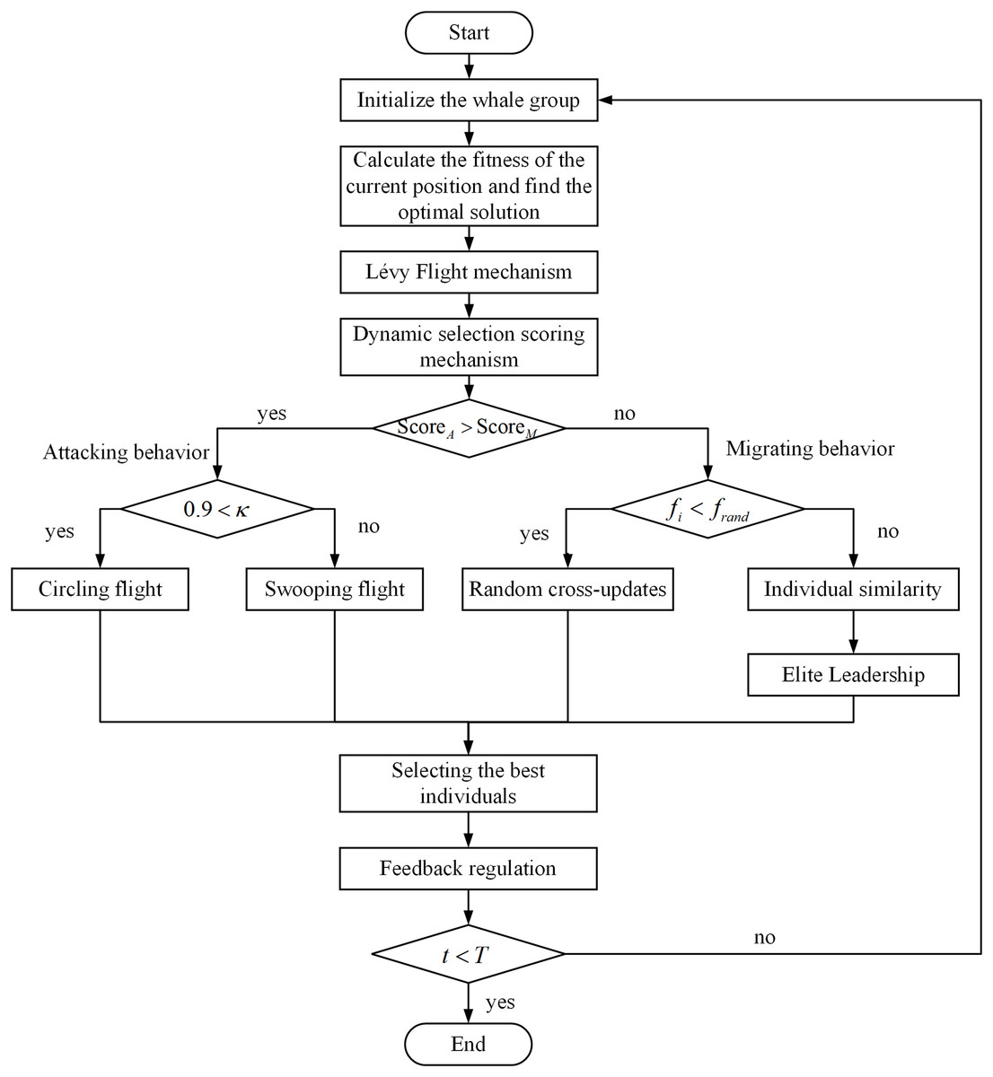
Figure 3: Schematic diagram of PO-MIBKA process.
Initialization of PO-MIBKA: The first step in initializing the population is to create a set of random solutions, where the position of each individual black-winged kite is represented by a matrix. Assuming a population size of and a problem dimension size of , the -th dimensional position of the -th black-winged kite can be represented as .
(35)
The location of each black-winged kite is usually distributed evenly over a range.
(36) where , and are the lower and upper bounds of the -th dimension, respectively, and rand is a randomly chosen value between 0 and 1.
After initializing the position, the fitness value of each individual is calculated and the individual with the smallest value is taken as the leader.
(37)
is the optimal location for this population at the time .
Attack behavior: The capture of prey by black-winged kites is usually divided into two phases: circling flight in search of prey and swooping flight to feed on prey.
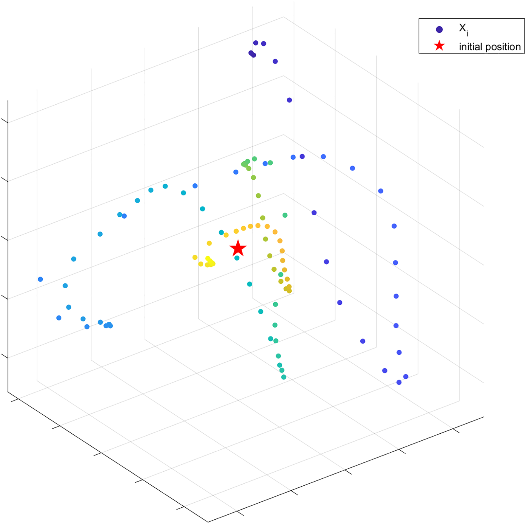
The formula for calculating black-winged kites circling for prey in the traditional BKA causes the update position to appear only in the upper right of the most advantageous point, and does not achieve a circling effect. To solve the above problem, we introduce a spiral factor to update the position. Assuming an iteration period of , the possible update positions in the hovering behavior are shown in Fig 4.
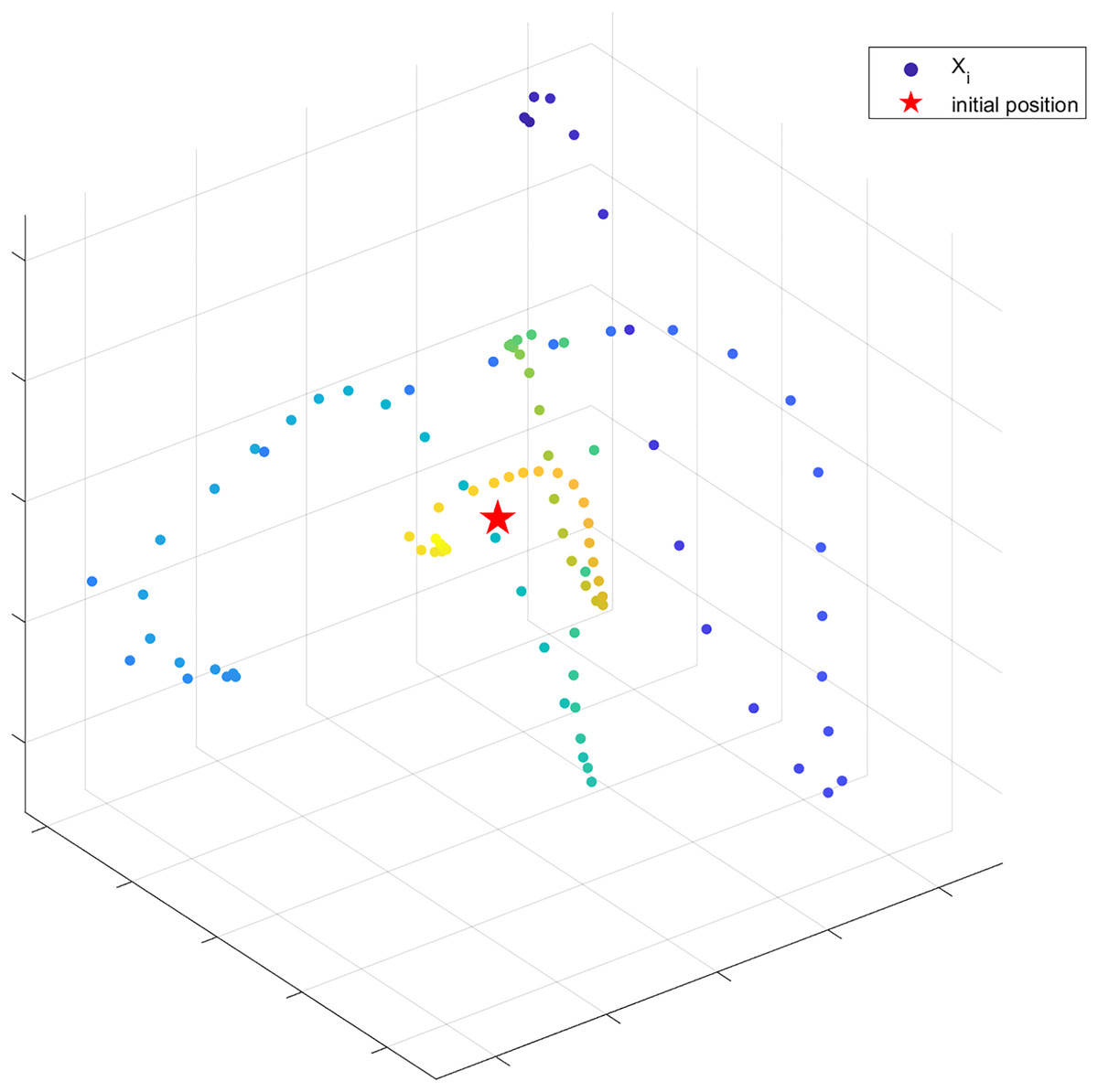
Figure 4: Possible update locations for hovering behavior.
Assume is a random number. If , the position is updated when hovering as follows:
(38)
(39) where is the dynamic radius and is the spiral factor.
(40) where are the frequency parameters of each dimension that control the spiral shape.
If , the black-winged kite makes a swooping attack. This action causes the status to be updated to:
(41)
Migration behavior: In order to better adapt to change seasons, many birds migrate from north to south during winter to obtain better living conditions and resources. During the migration process, a leader will usually lead the group. The navigational ability of the leader is crucial to the success of the entire group in completing the migration. When the fitness value of the current population exceeds that of the randomly generated population, the leading individual will guide the population to move forward until reaching the target destination. Conversely, when the fitness value of the current population is lower than that of the random population, the leader abdicates its guiding role, and the population migration process is regulated by the proposed stochastic cross-updating mechanism. The model for population migration is described as follows:
(42)
When , the model is updated in a manner consistent with Eq. (20). C is the Corsi mutation.
(43) where and .
The above are the three main steps of PO-MIBKA, the pseudo code is shown in Algorithm 1.
| Initialization: . |
| Calculation of the adaptation: . |
| Determination of the optimal: |
| while do |
| Lévy Flight mechanism: |
| Calculation: |
| Calculation: |
| if then |
| if then |
| else |
| end if |
| else |
| if then |
| else |
| end if |
| end if |
| end while |
| return |
Function test on PO-MIBKA
A comparison is made between PO-MIBKA and traditional BKA on classical test functions. The number of iterations for optimization of each function is 1,000 and optimal fitness curves are shown in Fig. 5
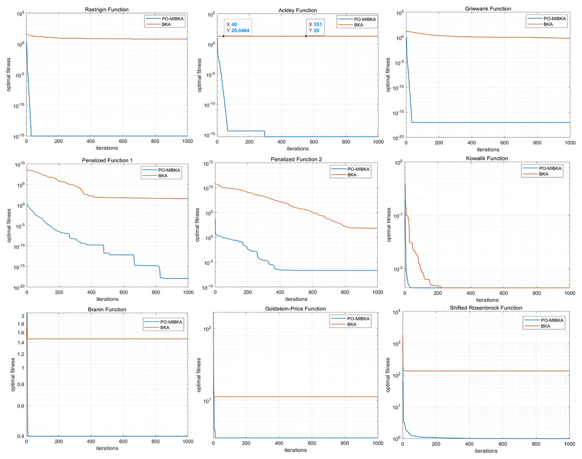
Figure 5: The optimal fitness curves of PO-MIBKA and BKA.
The improved PO-MIBKA achieves a faster optimization search speed than the traditional BKA algorithm and significantly improves its ability to find the global optimal solution or a better solution. The comparison of the optimal fitness values of the test functions at 1,000 iterations is shown in Table 1.
| Function | Rastrigin | Ackley | Griewank | Penalized 1 |
| PO-MIBKA | 1.00e−15 | 4.44e−16 | 1.00e−17 | 1.31e−18 |
| BKA | 5.97 | 20.00 | 0.52 | 32.86 |
| Function | Penalized 2 | Kowalik | Branin | FGoldstein-Price |
| PO-MIBKA | 2.30e−07 | 4.40e−2 | 0.40 | 3.00 |
| BKA | 64.85 | 4.40e−2 | 1.47 | 11.22 |
| Function | Shifted Rosenbrock | |||
| PO-MIBKA | 0.36 | |||
| BKA | 280.70 |
Complexity analysis
Based on the position update and fitness calculation mechanism of the PO-MIBKA algorithm, assume the complexity of the fitness function Fit( ) is , the search space dimension is , the population size is , and the maximum number of iterations is T. In the initialization phase, the algorithm generates initial solutions and calculates their fitness, with a complexity of . In the main loop, each iteration includes the Lévy flight mechanism, score calculations, position updates under conditional judgment, and the best solution update. Among these, the Lévy flight and position update operations involve vector computations with a complexity of ; fitness calculation and score calculations require traversing the population, resulting in a complexity of . Since the operations in the conditional branches are all related to the population size and dimension, the worst-case complexity per iteration is . Therefore, the overall time complexity is .
Simulation and experiments
For real-time UCAVs path planning under dynamic RCS constraints, we performed three sets of experiments to verify the reliability of the algorithm. These simulations propose a scenario-adaptive trajectory optimization framework for UCAVs to dynamically modulate their RCS characteristics, thus probabilistically evading adversarial radar detection locks and ensuring successful penetration missions. Through multiobjective evolutionary algorithms, flight trajectories are reconfigured in real time in various threat environments, achieving a reduction of at least in average radar detection probability compared to conventional path-planning methods. The parameters required for real-time trajectory planning are shown in Table 2. All of these parameters are used in the following three cases.
| Parameters | |
|---|---|
| Battlefield mission space | {xmax = 60 km, ymax = 60 km} |
| Attack angle | |
| Roll angle | |
| Air density | 1.225 km/m3 |
| Gravitational acceleration | 9.8 m/s2 |
| Equivalent cross-sectional area S | 49.24 m2 |
| Weight of UCAV | 14,680 kg |
| Real-time detection radius | 30 km |
Case 1: A comparative evaluation of UCAV trajectories before and after optimization was performed in a planar terrain configuration scenario with a single static radar threat source to quantify the effectiveness of the proposed algorithms in reducing the probability of locking on radar detection. The locations of the UCAV and the radar in case 1 are shown in the Table 3.
| Coordinate | |
|---|---|
| UCAV takeoff position | (5, 12, 0) |
| Target position | (50, 36, 0) |
| Radar station position | (23, 39, 0) |
Figure 6 shows the results of trajectory planning considering dynamic RCS. In order to effectively avoid the risk of radar detection locking, the proposed dynamic RCS-based trajectory planning enables the UCAV to adopt a circuitous route instead of a line traversal, which is used to circumvent the radar detection range. This tactic significantly reduces the risk factor of being tracked by maintaining a safe distance from the radar station and keeping the dynamic RCS at a minimum.
Figure 6: Comparison of penetration planning incorporating and neglecting dynamic RCS in case 1.
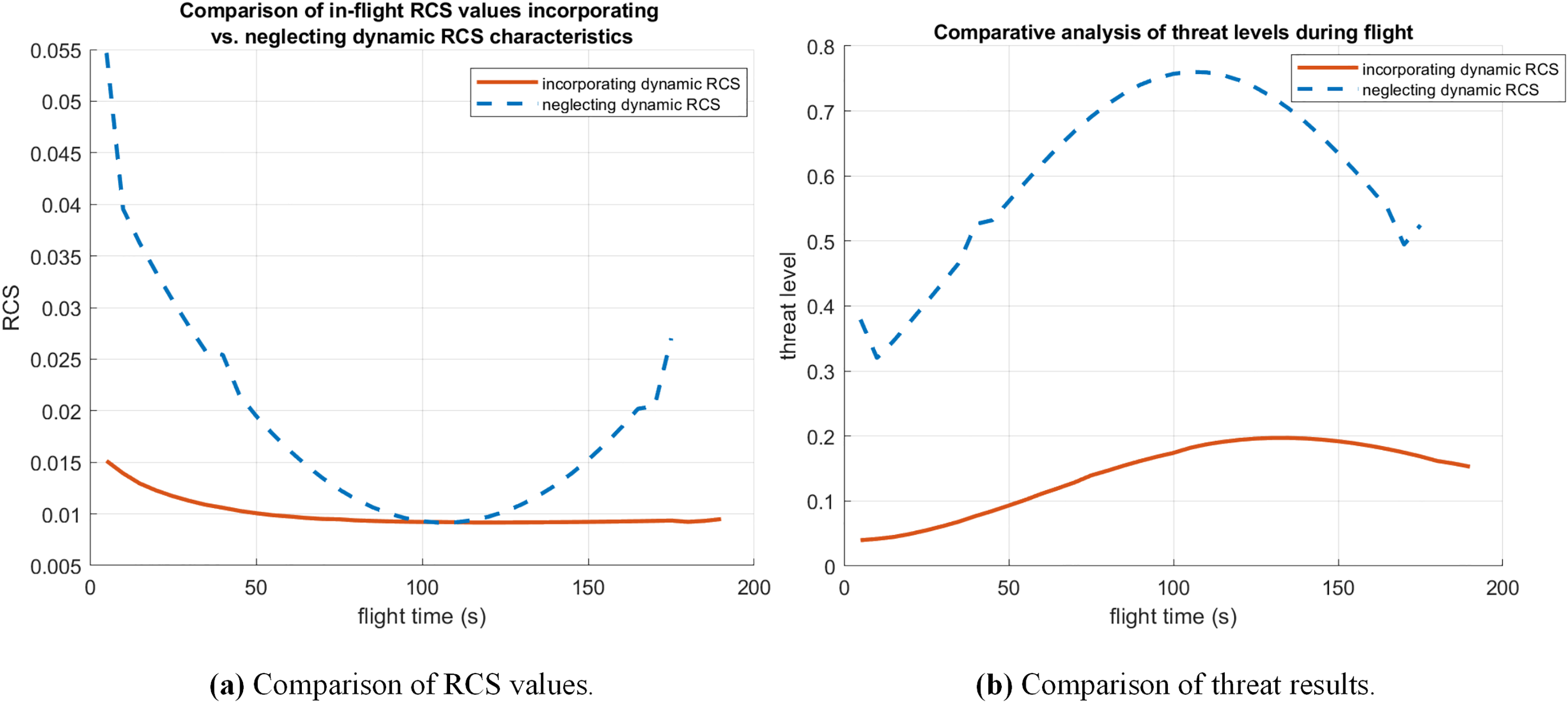
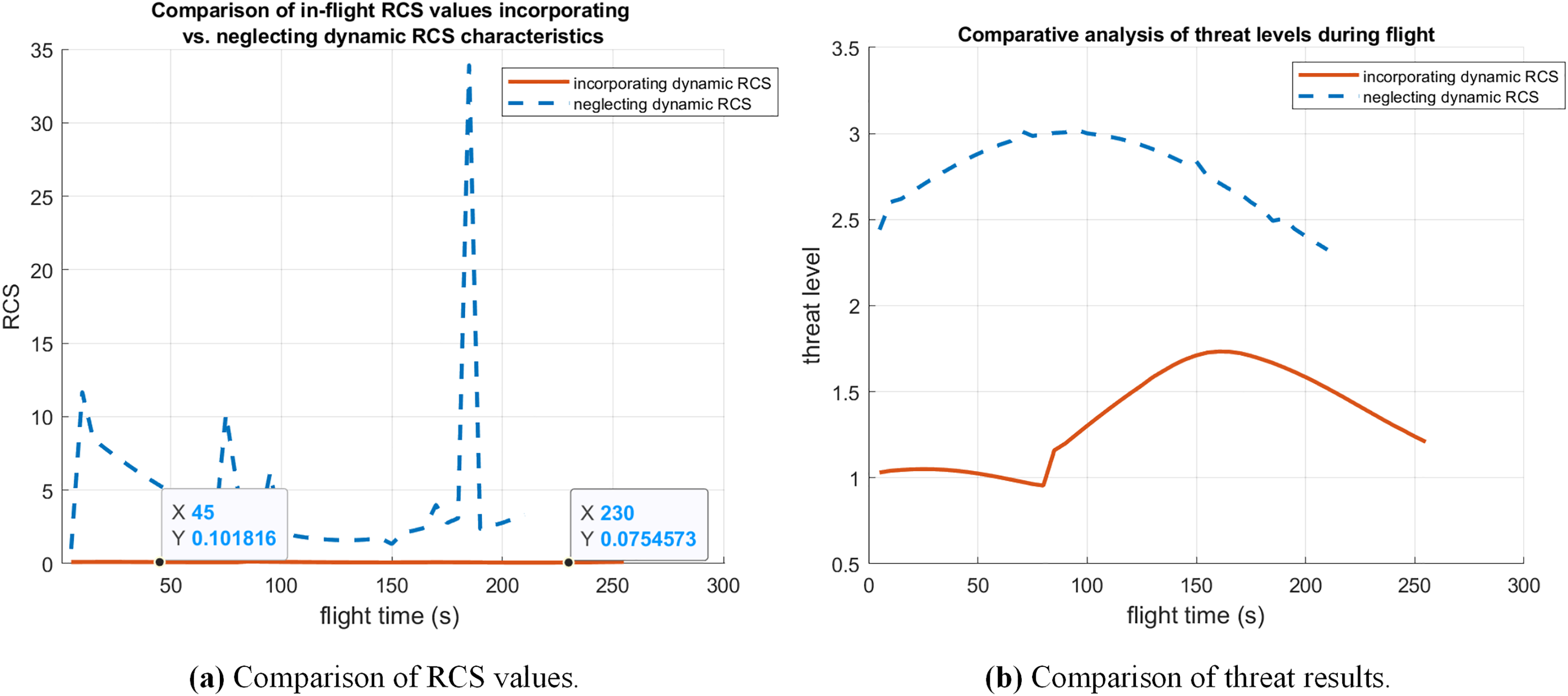
The variations of dynamic RCS values and the probability of radar threat received under two flight trajectories are shown in Fig. 7. It is obvious that this trajectory planning strategy successfully achieves the tactical goal of suppressing radar locking through flight path optimization while safeguarding the electromagnetic concealment of the UCAV. Quantifying the risk aversion effect of proposed vehicle planning algorithms (Table 4). The average RCS is reduced by compared to conventional path planning methods. At the same time, the radar threat is reduced by .
Figure 7: Comparison of RCS values and threat results in case 1.
| Incorporating dynamic RCS | 0.0100 | 0.1400 |
| Neglecting dynamic RCS | 0.0187 | 0.6047 |
Additionally, we compare the optimal path results obtained by the proposed PO-MIBKA algorithm and the traditional BKA algorithm in case 1. The comparison results are shown in the Table 5. The data in the table shows that when considering dynamic RCS, the proposed algorithm performs better than traditional BKA.
| Path length | Computation time | |
|---|---|---|
| PO-MIBKA-RCS | 50.3200 | 44.8779 |
| BKA-RCS | 51.7356 | 48.3765 |
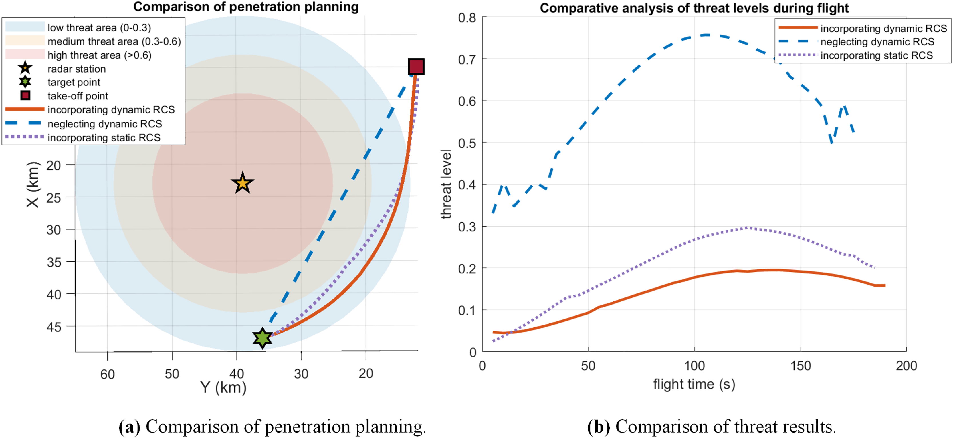
Furthermore, comparing static RCS and dynamic RCS as distinct constraints, the method for establishing static radar cross section models involves data table interpolation. Due to differences in the implementation of the RCS model as a constraint condition, we only compared the obtained paths and the results of the threats encountered. The results are shown in the Fig. 8.
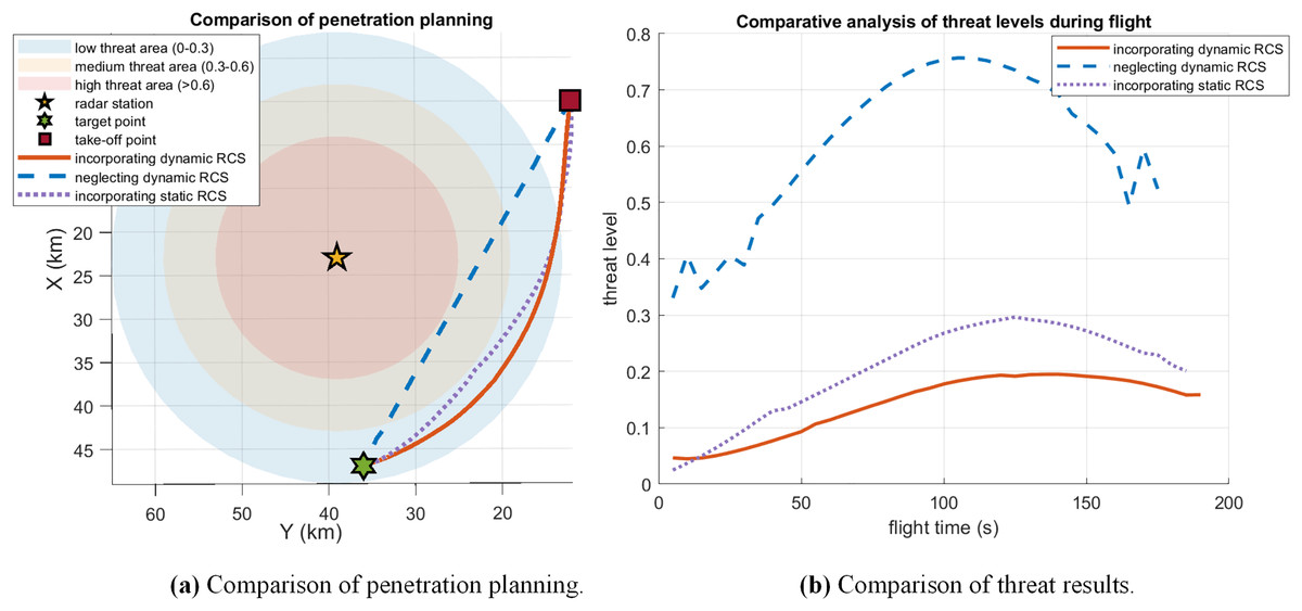
Figure 8: Comparison of dynamic RCS and static RCS in case 1.
In this case, the path obtained by the PO-MIBKA algorithm considering static RCS can deviate from the radar but still poses a significant threat.
Case 2: Increased radar threat leads to more complex penetration missions. Evaluate the anti-detection performance of the proposed algorithm in a multi-radar collaborative electromagnetic environment (three radars). The locations of the UCAV and the radar in case 2 are shown in the Table 6.
| Coordinate | |
|---|---|
| UCAV takeoff position | (5, 12, 0) |
| Target position | (50, 55, 0) |
| Radar Station 1 position | (15, 31, 0) |
| Radar Station 2 position | (56, 27, 0) |
| Radar Station 3 position | (34, 60, 0) |
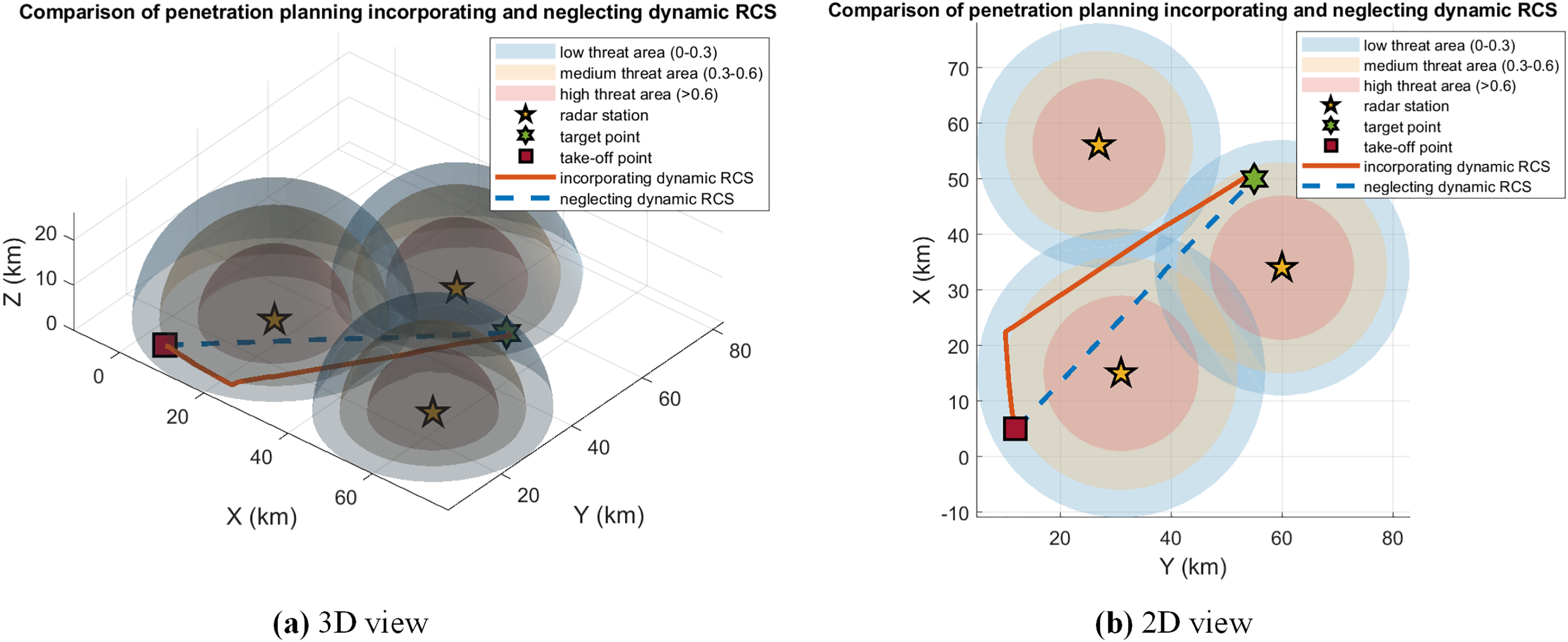
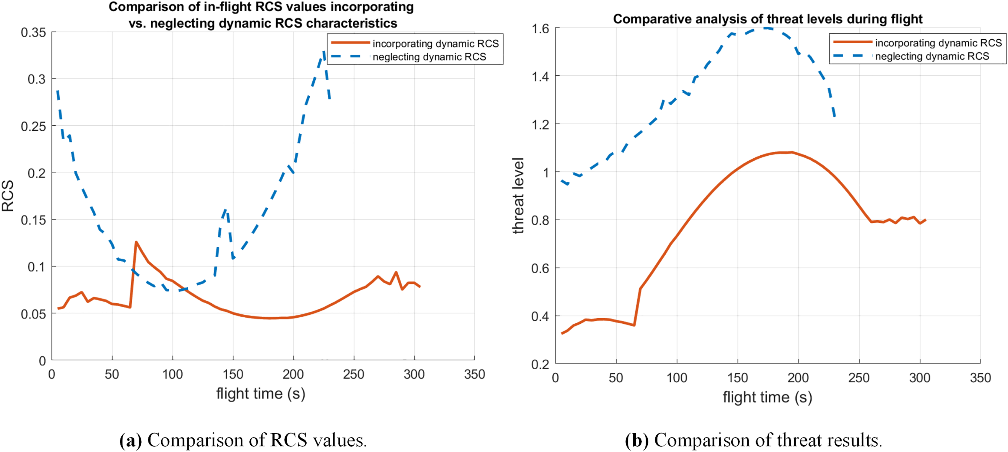
The comparison of penetration planning incorporating and neglecting dynamic RCS is shown in Fig. 9. Dynamic RCS-based trajectory planning generates results as orange curves. It is obvious that the UCAV chose to fly in the middle of the three radars to avoid an increase in RCS. The comparisons of dynamic RCS values and the probability of radar threat received under two flight trajectories are shown in Fig. 10. The trajectory without considering dynamic RCS has an RCS value of under the influence of radar 1, which is much higher than the trajectory after risk aversion. The required trajectory reduces the RCS value in the preexisting period under the influence of radar 3. Although the RCS due to radar 2 is larger, the total real-time dynamic RCS value of the UCAV is much lower than that of the trajectory without considering dynamic RCS.
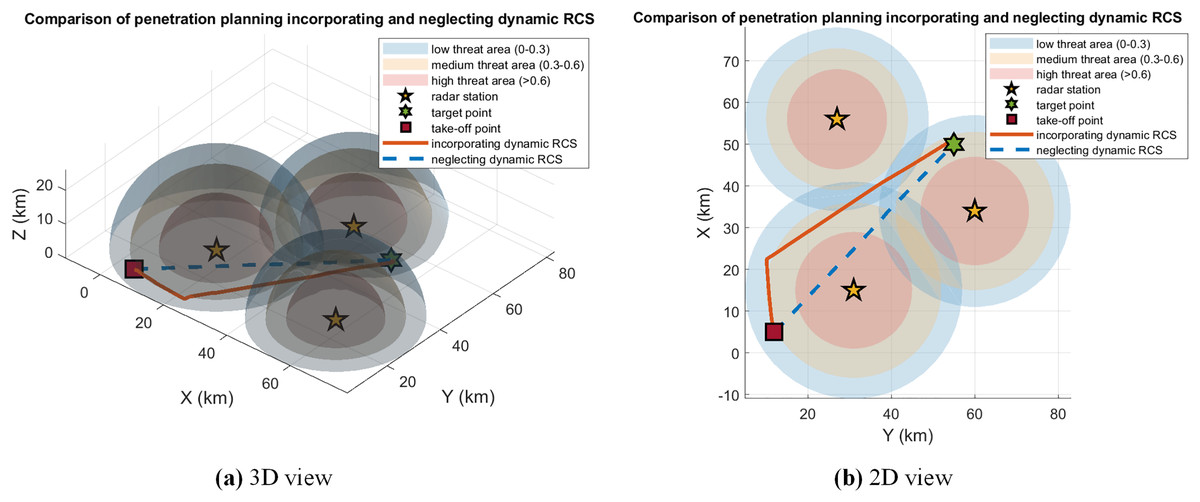
Figure 9: Comparison of penetration planning incorporating and neglecting dynamic RCS in case 2.
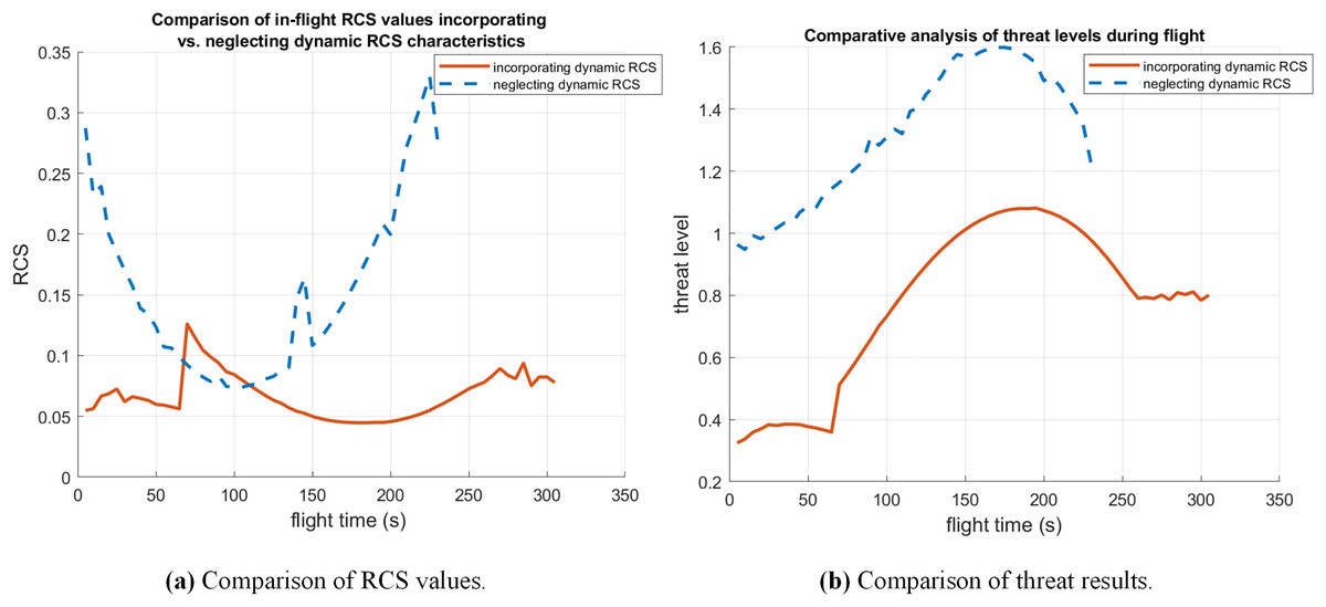
Figure 10: Comparison of RCS values and threat results in case 2.
The trajectory obtained by the PO-MIBKA considering dynamic RCS exhibits an average RCS of , whereas the trajectory generated by the standard PO-MIBKA without RCS consideration yields a significantly higher average RCS of (see Table 7). The average RCS is reduced by compared to conventional path planning methods. At the same time, the radar threat is reduced by .
| Incorporating dynamic RCS | 0.0670 | 0.7766 |
| Neglecting dynamic RCS | 0.1536 | 1.3232 |
In case 2, both the PO-MIBKA and traditional BKA algorithms account for dynamic RCS. The results for optimal path length and computation time obtained during operation are shown in Table 8.
| Path length | Computation time | |
|---|---|---|
| PO-MIBKA-RCS | 67.9815 | 120.3765 |
| BKA-RCS | 68.7619 | 122.0182 |
The data in the table indicates that, when accounting for dynamic radar cross section, the proposed PO-MIBKA algorithm achieves shorter computation times and path lengths.
Similarly, using the static RCS design method from case 1, simulations were conducted for case 2 under both dynamic RCS and static RCS constraints. The results are shown in the Fig. 11.
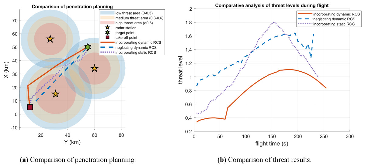
Figure 11: Comparison of dynamic RCS and static RCS in case 2.
Dynamic RCS, when applied as a path planning constraint, enables real-time adaptation to battlefield environment changes. By adjusting flight paths and aircraft attitude, it minimizes radar detection risk. Compared to static RCS or ignoring RCS, this approach offers greater flexibility and adaptability. Paths incorporating dynamic RCS not only avoid high-threat zones but also reduce sustained threat levels, thereby enhancing the survivability and success rate of penetration missions.
Case 3: A more complex penetration scenario is designed to rigorously evaluate the performance of the proposed path planning algorithm under challenging conditions. This scenario integrates a network of five heterogeneous radar systems, strategically deployed to create overlapping threat zones. The specific geographic locations and operational parameters of the UCAV’s starting point, designated target, and all five radar sites are detailed in Table 9. This configuration aims to test the algorithm’s ability to evade multiple threats.
| Coordinate | |
|---|---|
| UCAV takeoff position | (8, 6, 0) |
| Target position | (47, 50, 0) |
| Radar Station 1 position | (18, 20, 0) |
| Radar Station 2 position | (44, 22, 0) |
| Radar Station 3 position | (15, 60, 0) |
| Radar Station 4 position | (38, 42, 0) |
| Radar Station 5 position | (30, 5, 0) |
The comparison of penetration planning incorporating and neglecting dynamic RCS is shown in Fig. 12. This comparison clearly reveals that neglecting dynamic RCS characteristics leads to substantially higher predicted detection probabilities along the trajectory. Accurate RCS modeling is therefore critical for generating feasible low-observability paths.
Figure 12: Comparison of penetration planning incorporating and neglecting dynamic RCS in case 3.
A quantitative comparison of the RCS values and radar detection probability, as delineated in Fig. 13 and Table 10, unequivocally demonstrates the superiority of the proposed approach. The results reveal a staggering 97.92 reduction in the average RCS when compared to conventional path planning methods. This dramatic suppression of the aircraft’s radar signature directly translates into a substantial operational advantage, manifesting as a 51.47% decrease in the integrated radar threat probability throughout the penetration mission. This significant mitigation of detection risk markedly enhances the likelihood of mission success and survivability.
Figure 13: Comparison of RCS values and threat results in case 3.
| Incorporating dynamic RCS | 0.0941 | 1.3471 |
| Neglecting dynamic RCS | 4.5242 | 2.7756 |
Similarly, comparing the path length and computation time of the PO-MIBKA and traditional BKA algorithms in case 3 yields the results shown in Table 11.
| Path length | Computation time | |
|---|---|---|
| PO-MIBKA-RCS | 73.4400 | 490.6411 |
| BKA-RCS | 76.1384 | 531.5243 |
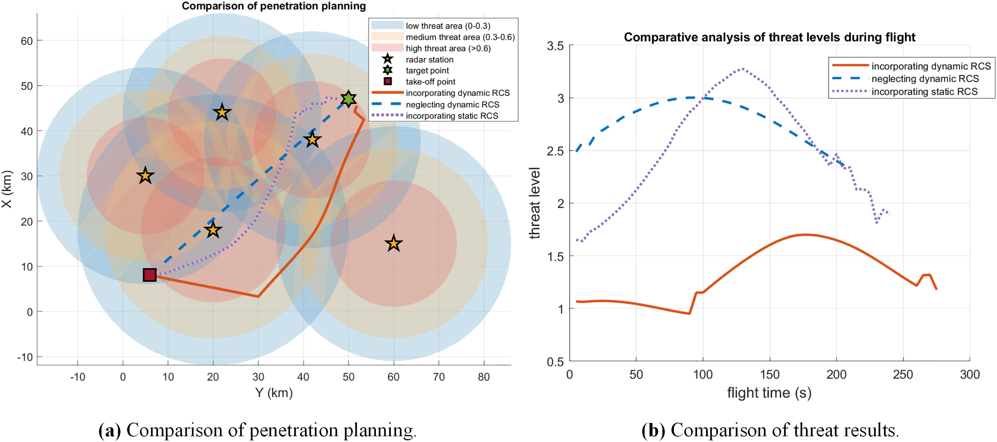
To ensure a consistent comparison across scenarios, the static RCS design methodology established in case 1 was applied as a benchmark in case 3. A comprehensive simulation was then conducted, contrasting the outcomes of this static RCS approach against those obtained under dynamic RCS constraints. The comparative results of these two planning strategies are presented in Fig. 14. The results indicate that path planning with dynamic RCS constraints can effectively avoid high-threat areas and maintain a lower threat level throughout the entire flight.
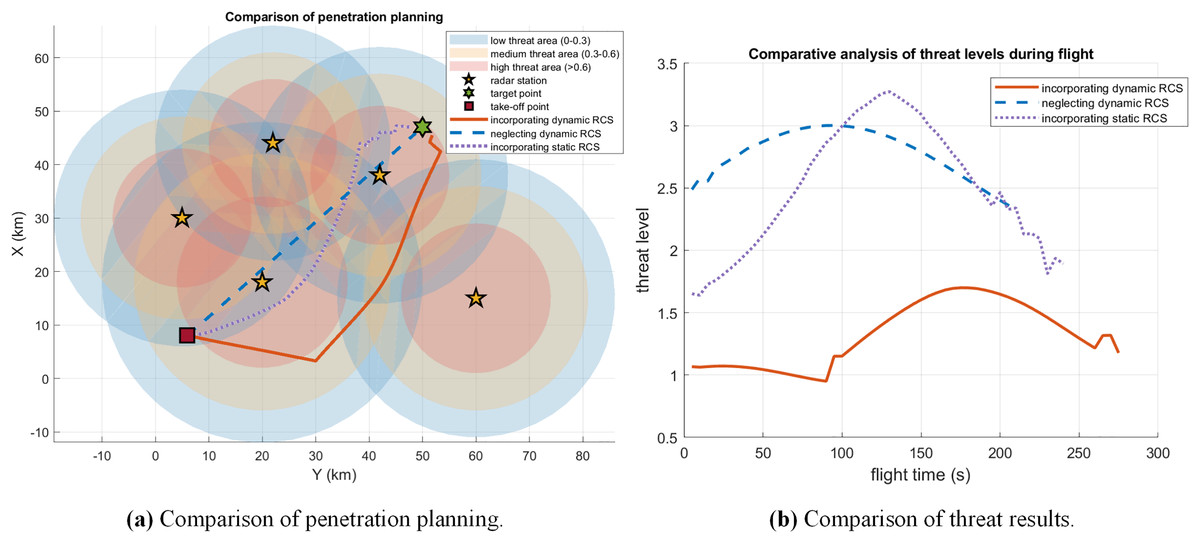
Figure 14: Comparison of dynamic RCS and static RCS in case 3.
Conclusion
The dynamic RCS-aware PO-MIBKA proposed in this study optimizes the generation of low-observable trajectories by calculating RCS changes in real time. Simulation results show that the algorithm can effectively reduce the average RCS by at least compared with the traditional trajectory planning methods, and at the same time satisfy the mission constraints such as flight time and path. The algorithm ensures that the UCAV always has a low RCS during flight, which significantly improves the penetration capability. In addition, the algorithm has fast convergence and low computational overhead, making it suitable for real-time mission planning in complex battlefield environments.
Future work could provide insights for more complex flight conditions, such as considering UCAV skin surface damage leading to high RCS at specific angles. In addition, deep reinforcement learning could be introduced in conjunction with dynamic RCS-based trajectory planning. Finally, different UCAVs are modeled differently, which leads to different models for dynamic RCS, and we will soon attempt to build a real-time RCS dynamic database instead of building a model to obtain a more accurate relationship between RCS, radar, and UCAV attitude.