
Energy awareness prediction model based on multi-agent decision-making modeling in green supply chain marketing strategy
- Published
- Accepted
- Received
- Academic Editor
- Muhammad Asif
- Subject Areas
- Algorithms and Analysis of Algorithms, Artificial Intelligence, Data Mining and Machine Learning, Data Science, Natural Language and Speech
- Keywords
- Green supply chain, Energy awareness prediction, Multi-agent decision-making, Evidence theory, K-means clustering, BiLSTM
- Copyright
- © 2026 Chen
- Licence
- This is an open access article distributed under the terms of the Creative Commons Attribution License, which permits unrestricted use, distribution, reproduction and adaptation in any medium and for any purpose provided that it is properly attributed. For attribution, the original author(s), title, publication source (PeerJ Computer Science) and either DOI or URL of the article must be cited.
- Cite this article
- 2026. Energy awareness prediction model based on multi-agent decision-making modeling in green supply chain marketing strategy. PeerJ Computer Science 12:e3440 https://doi.org/10.7717/peerj-cs.3440
Abstract
In the context of the “dual carbon” strategy and sustainable development, the green supply chain marketing strategy has become an essential means to guide enterprises and consumers to form awareness of energy conservation and emission reduction. This article proposes a Bidirectional Long Short-Term Memory (BiLSTM) prediction model structure that integrates evidence theory and K-means clustering to address the complex and dynamic modeling of energy awareness in multi-agent participation, and constructs an energy awareness prediction model for green supply chains. Firstly, utilizing evidence theory to fuse multi-source information enhances the ability to handle data uncertainty and decision robustness. Subsequently, the K-means algorithm was used to cluster the historical behavior data of different entities in the supply chain and identify typical energy behavior patterns. Finally, based on the clustering results, a BiLSTM prediction model is constructed to explore temporal behavior characteristics and predict and analyze the energy awareness evolution trends of different entities under green marketing strategy intervention. The experimental results show that compared with models such as CNN BiLSTM, the method proposed in this article has reduced Root Mean Square Error (RMSE) and Mean Absolute Error (MAE), while the upper limit of relative error does not exceed 8%.
Introduction
With the increasing severity of global climate change and resource and environmental issues, green supply chain management has become a key path to promote sustainable development. While pursuing economic benefits, enterprises are increasingly emphasizing energy efficiency, environmentally friendly production methods, and the improvement of consumers’ green awareness. Especially under the guidance of the “dual carbon” target, how to achieve collaboration and interaction among various entities in the upstream and downstream of the supply chain on green goals has become an important issue that urgently needs to be addressed (Shen & Wang, 2024).
Accurately predicting key variables such as energy demand, consumption preferences, environmental impact factors, etc., in green supply chain management is the foundation for achieving scientific decision-making and optimizing resource allocation. The commonly used prediction methods currently include traditional time series analysis and intelligent modeling techniques based on machine learning. In recent years, deep learning models such as recurrent neural networks (RNNs) and convolutional neural networks (CNNs) have demonstrated excellent predictive performance in fields such as cold chain management and inventory control (Cheng & Yang, 2021; Semenoglou, Spiliotis & Assimakopoulos, 2023). For example, Meng et al. (2024) constructed an efficient stock index prediction model by combining an improved bacterial foraging optimization algorithm (BFO) with a Bayesian network, verifying the practicality of deep models in predicting complex variables.
The many variables in green supply chains often have obvious temporal dependencies and dynamic evolution characteristics, making their prediction problems essentially belong to the category of time series modeling. Long short-term memory network (LSTM), as a typical variant of RNN, is widely used in tasks such as lifecycle prediction and price trend judgment due to its advantages in modeling long-term dependency problems. Park et al. (2020) used LSTM to predict the lifespan of lithium batteries, and the results significantly reduced the risk of battery failure. Nelson, Pereira & De Oliveira (2017) used the LSTM model to predict stock price trends, achieving an average accuracy of 55.9%. Tsironi et al. (2017) used LSTM to model the temperature changes of green leaf salad in cold chain environments, which outperformed traditional methods under various conditions.
On this basis, this article introduces a bidirectional long short–term memory network (BiLSTM) to improve the performance of the model further. Compared with traditional LSTM, BiLSTM can extract features from both forward and backward directions of time series, capture contextual information more comprehensively, and improve the modeling ability of complex time-dependent structures. It is particularly suitable for highly nonlinear and dynamic prediction tasks such as energy awareness changes and multi-agent behavior feedback in green supply chains. To further improve prediction accuracy and model robustness, this article integrates K-means clustering and evidence theory and constructs a clustering evidence fusion deep model (K-BiLSTM) based on BiLSTM. This model integrates class preprocessing, information fusion, and sequence learning, and can effectively identify the behavioral characteristics of the subject and dynamically model its green consciousness evolution process.
Related works
In recent years, deep learning has shown strong performance in tackling real-world prediction tasks, especially time series forecasting. Businesses leverage these models to mine consumer patterns and enhance marketing decisions. Accurate sales forecasting has thus become essential for optimizing strategies and driving future growth. The success of deep learning has also accelerated the advancement of machine learning as a whole. Deep learning outperforms traditional methods in key machine learning areas like natural language processing (NLP) (Zheng et al., 2025), image analysis (Deng, Zhang & Shu, 2018), and speech synthesis (Irshad, Gomes & Kim, 2023). For example, Yongsheng & Yingquan (2025) used time series models to extract market signals for predicting future price movements.
Based on the field of deep learning, the processing capabilities of different neural network models are analyzed. With the ability of LSTM to fully consider the temporal data sequence relationship, more and more scholars (Verma & Chafe, 2021; Black & Scholes, 2019) were inputting the effective features extracted by CNN into LSTM to construct a CNN-LSTM combination model. Improved and enhanced validated models, such as Generalized Autoregressive Conditional Heteroskedasticity (GARCH), using machine learning components such as artificial neural networks (Baek, 2024; Zhang et al., 2024). Adopting new hybrid models and neural networks to improve the original performance (Song & Choi, 2023). In Kristjanpoller & Michell (2018), and Xu, Yang & Alouini (2022), neural networks were used to predict future exchange rates. The model was tested for daily and annual predictions, and the conclusion was drawn that short–term predictions are more accurate. Beniwal, Singh & Kumar (2023) proposed a deep portfolio theory that utilizes autoencoders to generate optimal investment portfolios.
However, traditional LSTM models only consider the unidirectional relationship of time (Abedin et al., 2025), lacking consideration for the bidirectional relationship of time. Soleymani & Paquet (2020) used the BiLSTM bidirectional neural network model to predict the S&P500 dataset, and empirical results showed that the prediction accuracy of the BiLSTM model was higher than that of CNN and LSTM. The bidirectional LSTM model fully utilizes the relationship between the forward and backward time dimensions of the time series, resulting in improved prediction accuracy. Meng et al. (2023), and Yang et al. (2024) introduced the BiLSTM model from deep learning into financial time series analysis, and the research results showed that the model performed the best in prediction accuracy. It can synchronously extract historical and future information features, taking into account the bidirectional dependence of data. Therefore, it has significant advantages in capturing short–term fluctuations and long-term trends in financial time series. Abduljabbar, Dia & Tsai (2021) proposed an atmospheric temperature prediction model based on a symmetric BiLSTM and an attention mechanism. This model utilizes BiLSTM to simultaneously extract forward and backward feature information in the time dimension, and introduces an attention mechanism to overcome the performance bottleneck of traditional LSTM in processing long time series, thereby achieving accurate prediction of atmospheric temperature and effectively improving the prediction accuracy of the model. Bhattacharjee, Kumar & Senthilkumar (2022), Lu et al. (2021) proposed a BiLSTM short–term prediction model based on phase space reconstruction, taking into account the chaotic characteristics of wind power sequences and meteorological data. This method enhances the modeling ability of BiLSTM for complex nonlinear relationships by reconstructing the dynamic characteristics of the original wind power time series, thereby effectively reducing the error of wind power prediction.
Materials and Methods
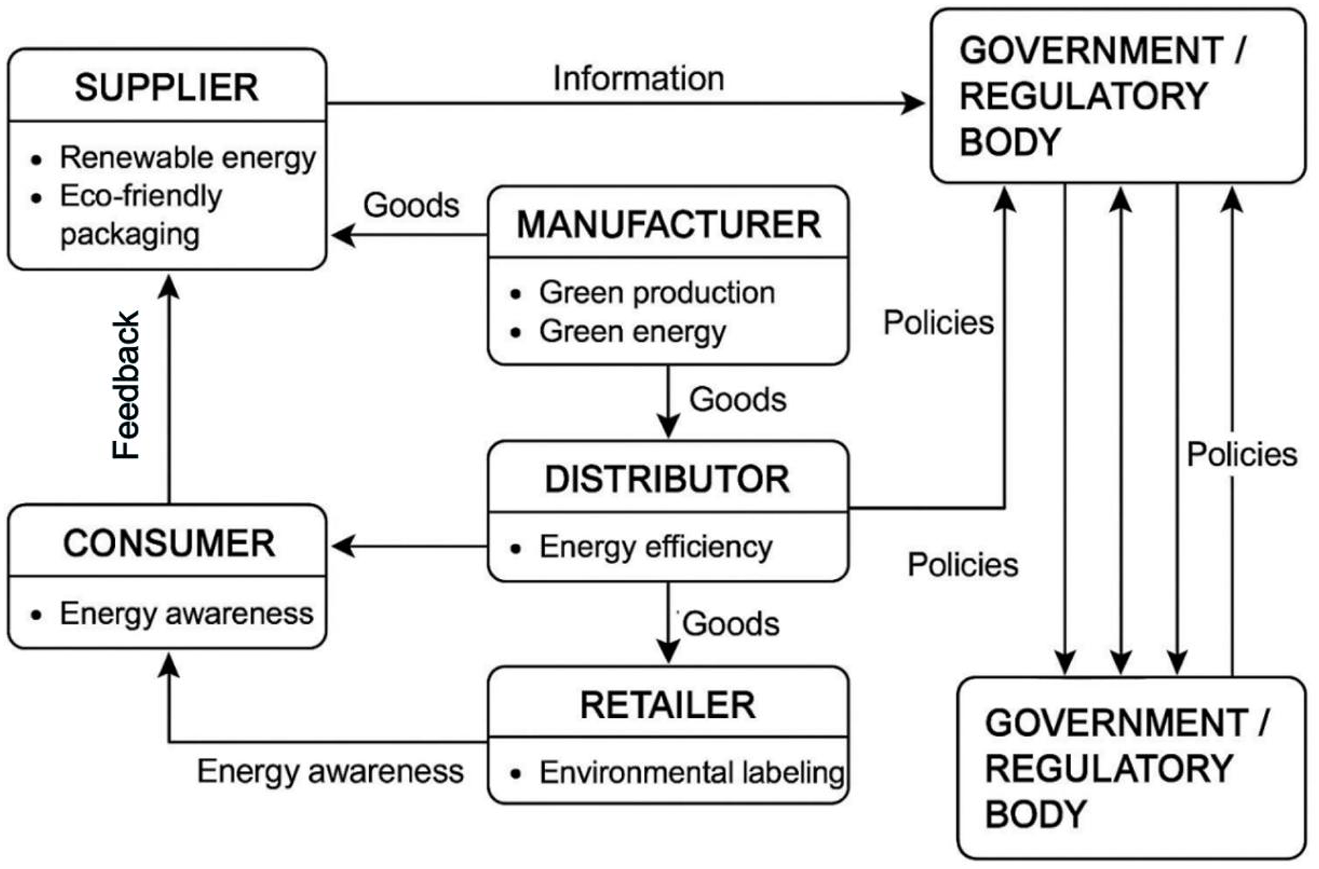
The structure of a green supply chain system involving multiple stakeholders is shown in Fig. 1, covering the interactive relationships between suppliers, manufacturers, distributors, retailers, consumers, and government/regulatory agencies. Each entity bears different green responsibilities in the circulation of goods. Suppliers provide renewable energy and environmentally friendly packaging, manufacturers focus on green production and green energy, distributors improve energy efficiency, retailers promote environmental labels, and consumers influence upstream enterprises through energy awareness and feedback. At the same time, government departments formulate relevant policies to regulate and guide the entire supply chain towards sustainable development, achieving a circular flow of information, goods, feedback, and policies among various entities.
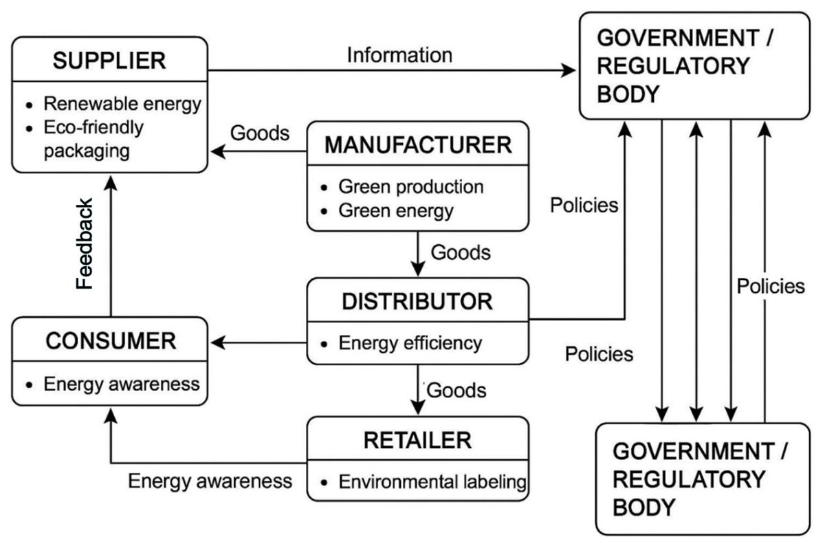
Figure 1: Multi stakeholder participation in green supply chain system structure.
To formally describe the multi-agent decision-making behavior in green supply chains, this article constructs the following mathematical model. The set of agents is defined as . The state of each agent at time t is represented by a vector , composed of its energy attributes and decision history. Interactions among agents are driven by a utility-based decision rule: the action of an agent depends on its own state and the joint state of its neighboring agents, i.e., , where the strategy aims to maximize its green utility function, .
Construction of multi-agent supply chain performance evaluation model
Building an evidence theory model
Evidence theory can merge information from different sources. In evidence theory, let evaluation indicator represent the j-th evidence in the i-th criterion layer, and represent the total number of evaluation indicators in the i-th criterion layer. represents the weight of the evidence at the i criterion layer, H represents the level set of evaluation indicators, represents the specific evaluation level, and represents the trustworthiness of evidence at evaluation level . Let the total evaluation value of the indicator be y.
Transformation based on utility theory
This article improves the use of the evaluation level performance value to distinguish the evaluation level from the utility level, as shown
(1) where represents the step size of value and represents the performance value set by the evaluation level after standardization, and is the nth normalized value.
Calculate the trustworthiness of belonging to using the equivalence rule. Let represent the value of the evaluation indicator , as , we can obtain:
(2)
In this way, the probability of the rating indicator being rated as evaluation level is , and the probability of being rated as is , namely .
Comprehensive evaluation based on evidence-based reasoning
(1) Calculate the initial trust value. Let be the basic probability allocation function of , representing the trustworthiness of the evaluation object am belonging to the evaluation level Hn, expressed as follows
(3) where is the weight coefficient.
(2) Evidence synthesis. Let represent the set of the first j pieces of evidence in the i-th layer, and be the comprehensive reliability of to . Use a nonlinear optimization model to calculate the fused confidence. According to the Dempster evidence combination process, fuse the evidence as shown
(4) where is the scaling factor used to indicate the degree of contradiction in the evidence.
(3) Use utility value mapping. Define as the expected utility value of for the overall evaluation, convert the evaluation value into a utility value, and use the result of the utility value as the final evaluation score for the supply chain, as shown
(5) Let and be two basic probability assignments on the same frame of discernment . For any proposition , , the combined basic probability assignment m(A) is calculated as follows:
(6) where the conflict coefficient K quantifies the total sum of all completely contradictory evidence combinations, defined as:
(7) The normalization factor 1/(1 − K) redistributes the probability mass assigned to the empty set proportionally to all consistent propositions, ensuring the combined result still satisfies the probability axioms.
Example 1: Let the frame of discernment be , representing “high energy awareness” and “low energy awareness,” respectively. Consider two pieces of evidence with the following basic probability assignments:
– Evidence 1:
– Evidence 2:
First, calculate the conflict coefficient:
(8) Then, compute the combined belief for proposition (H):
(9) Similarly, can be calculated. This example shows that although the two pieces of evidence are highly conflicting K = 0.74, the normalization process effectively preserves the weak consensus on hypothesis H from both sides and amplifies its relative weight from 0.1 to approximately 0.308, demonstrating the rule’s robust fusion capability under conflict.
BiLSTM multi-coupled energy prediction method based on K-means
Fuzzy clustering analysis based on K-means
K-means fuzzy clustering is a statistical method that classifies and organizes data samples based on the correlation between various factors. The steps are as follows:
(1) Assuming n observation samples, the sample set is: randomly select k samples as the initial clustering center .
(2) Calculate the Euclidean distance between each point in the sample and the initial cluster center point, and divide the nearest ones into the same category to form k clusters. The calculation formula is shown in Eq. (10)
(10)
Calculate the average of various samples and determine the new cluster center point.
Perform convergence judgment until the conditions are met, then clustering ends. Otherwise, return to step 2. The calculation formula is shown in Eq. (11)
(11) where is the collection of i-th class samples after the new clustering; is the object of sample ; is the center point of the -th cluster.
BiLSTM model
After K-means clustering, prediction is required. Neural network models are widely used in short–term load forecasting due to their strong self-learning and generalization abilities. The LSTM model can extract temporal information of loads and is more suitable for the field of energy prediction than traditional neural networks. The prediction model in this article is based on the BiLSTM model, which can simultaneously consider both forward and backward time information compared to the LSTM model, and better extract time series information.
The forward propagation process of LSTM
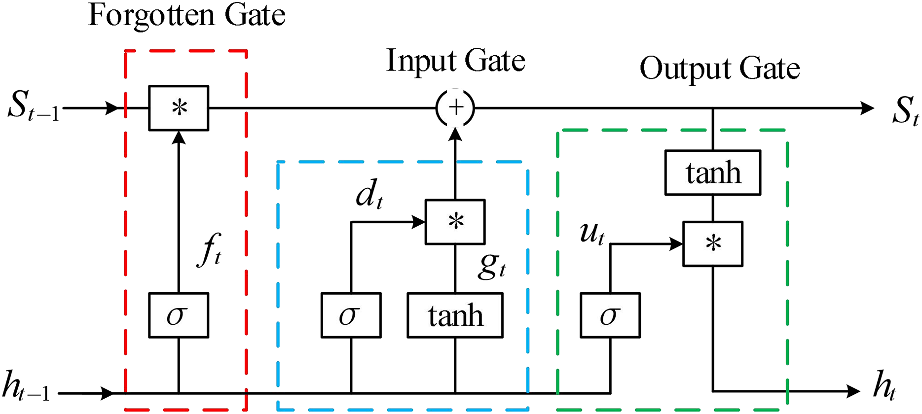
Compared to RNN, LSTM introduces the concept of “gates” to achieve long-term memory and solve gradient problems. The basic unit of LSTM is shown in Fig. 2.
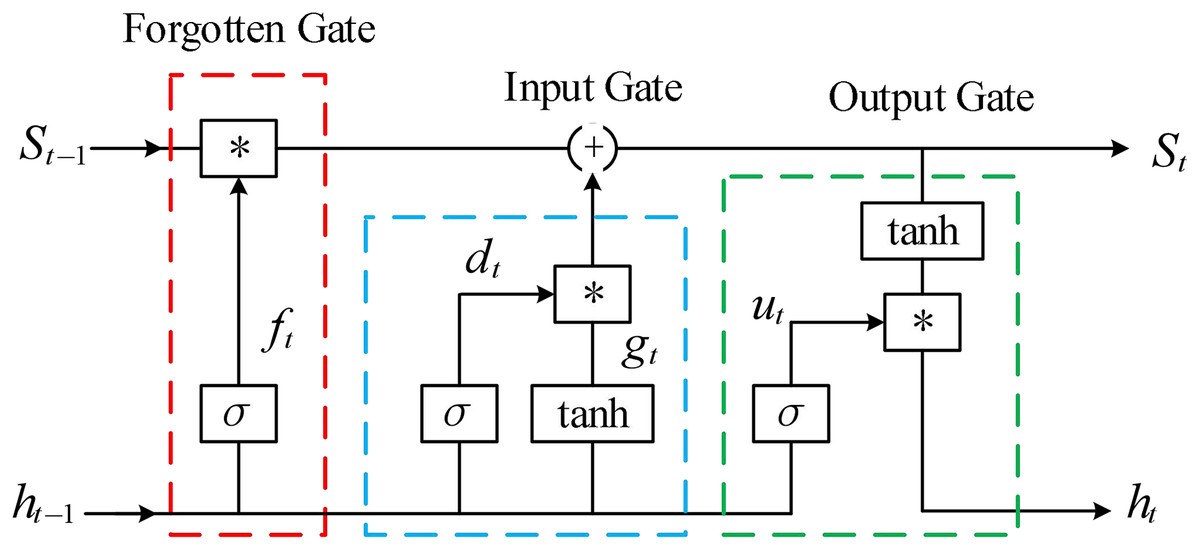
Figure 2: The basic unit of LSTM.
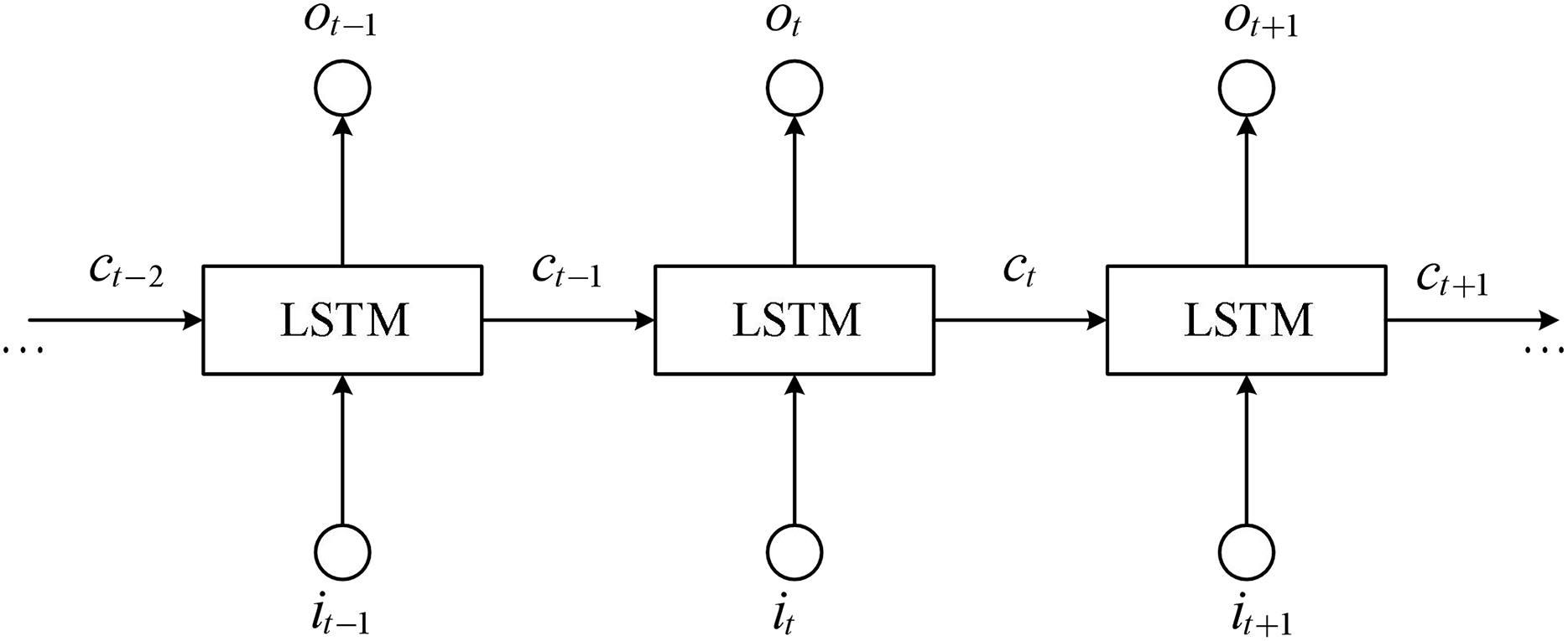
The schematic diagram of the structure of LSTM is shown in Fig. 3, where LSTM blocks are used to represent the basic units.
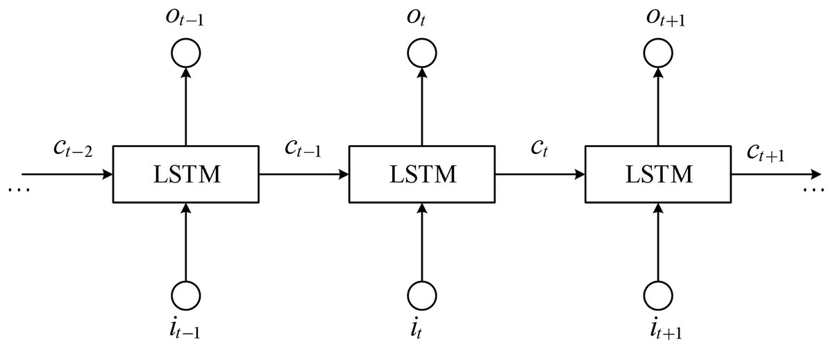
Figure 3: Structure diagram of LSTM.
The forget gate controls the memory function of historical time information, and LSTM controls the degree of forgetting of past time information through the forget gate. The calculation formula is shown in Eq. (12).
(12) where is the weight matrix of the forget gate, is the load forecast value at time t − 1, is the input feature at time t, is the bias matrix of the forget gate, and is the sigmoid function. The calculation formula is shown in Eq. (13).
(13)
The input gate determines which input data enters the LSTM, and the calculation formula is shown in Eq. (14).
(14) where and are the input gate weight matrix and input gate bias matrix, respectively.
The output gate is the last gate of the input state, used to control the amount of information transmitted to the external state . The calculation formula is shown in Eq. (15).
(15) where is the output gate weight matrix, is the output gate bias matrix, and is the output gate state at time t.
The internal information of LSTM is cyclically transmitted through memory units, while updating the external state . The calculation formulas are shown in Eqs. (16) and (17).
(16)
(17) where is the weight matrix of the memory unit, is the bias matrix of the memory unit, is the current input memory unit state, is the new memory unit state, is the state at t − 1, also known as the long-term memory state, and represents the element wise multiplication in the vector.
The final output update value of the LSTM basic unit is determined by the output gate and the state of the memory unit, and the calculation formula is shown in Eq. (18).
(18) where is the energy prediction value of LSTM unit at time t.
The forward propagation process of LSTM
The backpropagation process of LSTM is divided into three steps. Step one, at time t, calculate the partial derivatives of each gate according to Eq. (19).
(19)
Step two, calculate the partial derivative of the parameters in these gates according to Eq. (20).
(20)
Finally, calculate the partial derivatives of the hidden state, memory unit, and input according to Eq. (21).
(21)
By continuously adjusting the parameters of the LSTM neuron using the above formula, the error between the output value of the LSTM neural network and the true value becomes smaller and smaller until the predetermined accuracy is reached, and the training process ends.
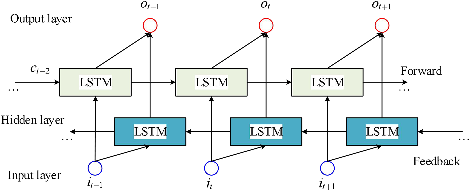
Working principle of BiLSTM
In energy forecasting, the energy at a later time also contains information about the energy at the earlier time; that is, the energy at a specific time is not only related to the load at the earlier time, but also to the energy at the later time. BiLSTM is composed of two directions of LSTM, one is forward LSTM and the other is backward LSTM. Forward LSTM can consider the information at the previous time, while backward LSTM can consider the information at a later time. Finally, the final prediction result is obtained by combining the two LSTMs.
The schematic diagram of the BiLSTM structure is shown in Fig. 4.
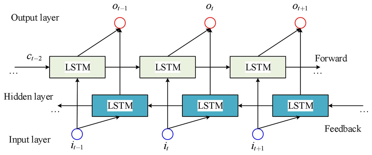
Figure 4: LSTM sequence display.
The calculation formula for BiLSTM is shown in (4.30)–(4.32).
(22)
(23)
(24) where is the energy prediction value at time t − 1, is the energy prediction value at time t + 1, and and are the energy prediction values of the forward and backward LSTM unit at time t, respectively. and are the forward and backward calculation processes of LSTM, and are the forward and backward output weights, is the bias optimization parameter at the current time, and is the final energy prediction value output by the BiLSTM unit at time t.
The model adopts an integration strategy of “clustering feature enhancement” rather than training independent sub-models. Specifically, K-means clustering is not applied to static enterprise profiles but to multi-variable time series segments processed via sliding windows. Its purpose is to identify distinct typical paradigms of energy consumption from the perspective of dynamic behavioral patterns. Each time series segment is assigned a corresponding cluster label, which is then concatenated with original multi-dimensional features such as energy consumption and marketing responses to form an enhanced feature vector, serving as the input to the BiLSTM network. In this way, clustering results are explicitly injected into the temporal model as crucial contextual information, guiding the BiLSTM to learn general temporal dynamics while adaptively capturing patterns specific to different behavioral types. This approach achieves a deep integration, shifting from a serial “sequence-clustering-prediction” pipeline to a cohesive “feature collaboration and end-to-end learning” framework.
Computing infrastructure
The computational experiments were performed on a high-performance workstation running Ubuntu 22.04 LTS as the operating system. The hardware included an Intel Core i9-13900K processor, 64 GB of RAM, and an NVIDIA RTX 4090 GPU with 24 GB VRAM, ensuring efficient processing of large datasets and deep learning models. The software environment utilized Python 3.10 with libraries such as TensorFlow 2.15 for BiLSTM implementation, scikit-learn for K-means clustering, and NumPy for data manipulation. Data storage was managed on a 1 TB SSD, with backups on a networked server to ensure data integrity during the training and evaluation phases.
Data preprocessing steps
Data preprocessing was a critical step to ensure the quality and usability of the multi-source datasets. Initially, raw data from supply chain entities were cleaned by removing outliers and missing values using a median imputation technique, followed by normalization to a [0, 1] scale to standardize features like energy consumption and marketing response rates. Categorical variables, such as entity type, were encoded using one-hot encoding. Time-series data were segmented into sequences of 30-day intervals to align with the BiLSTM input requirements, and a sliding window approach was applied to maintain temporal continuity. This preprocessing ensured compatibility with the clustering and prediction models, though no further transformation was applied post-clustering.
Evaluation method
The proposed energy awareness prediction model was evaluated using a comprehensive methodology that included both standard performance assessment and ablation experiments. The evaluation was conducted through a 5-fold cross-validation process on the preprocessed dataset, with 80% allocated for training and 20% for testing. Ablation experiments were designed to isolate the contributions of evidence theory, K-means clustering, and BiLSTM components by systematically removing each element and measuring the impact on predictive accuracy. This approach allowed for a robust assessment of the model’s effectiveness across different configurations, ensuring that comparative performance metrics justified the integration of these techniques.
Assessment metrics
The performance of the model was assessed using root mean square error (RMSE) and mean absolute error (MAE) as primary metrics, chosen for their sensitivity to prediction errors and alignment with the study’s focus on accurate energy awareness forecasting. RMSE, calculated as the square root of the average squared differences between predicted and actual values, emphasizes larger errors and is ideal for identifying significant deviations in trend predictions. MAE, the average absolute difference, provides a linear measure of error, offering a clear view of typical prediction accuracy. These metrics were selected to ensure a balanced evaluation of the model’s precision and reliability, with lower values indicating better performance, and their use was validated by comparing against baseline models like CNN-BiLSTM.
The complete workflow of the proposed K-BiLSTM method is shown in Algorithm 1.
| Input: Multi-agent raw time series data , number of clusters (K), BiLSTM hyperparameters |
| Output: *Predicted energy awareness sequence |
| 1. Data Preprocessing: |
| Clean X, handling missing values and outliers. |
| Normalize numerical features to the [0,1] range; apply one-hot encoding to categorical features. |
| Construct time series samples using the sliding window method. |
| 2. K-means Clustering: |
| Input the preprocessed time series sample set into the K-means algorithm. |
| Determine the optimal number of clusters K using the elbow method or silhouette score. |
| – Assign a cluster label l to each time series sample, forming an enhanced dataset . |
| 3. Evidence Theory Fusion: |
| If multi-source decision evidence exists, apply Dempster-Shafer theory for fusion. |
| Incorporate the resulting comprehensive confidence vector as additional features, combined with cluster labels into the feature set. |
| 4. BiLSTM Training and Prediction: |
| Split the enhanced dataset into training and test sets. |
| Construct a BiLSTM network, using both time series features and static features as input. |
| Train the BiLSTM model on the training set by minimizing prediction error. |
| Use the trained model to predict on the test set, obtaining the final energy awareness predictions . |
| 5. Output and Evaluation: |
| Evaluate model performance using RMSE and MAE. |
Experimental results
Experimental preparation
The research data is sourced from monthly panel data spanning 18 months (from January 2023 to June 2024) of 12 manufacturing enterprises in Region A of China, with a total sample size of 12 enterprises × 18 months = 216 records. The feature variables cover two categories: quantitative indicators and qualitative scores. Quantitative indicators include enterprise energy consumption, production output, sales revenue, etc., obtained through corporate financial reports and Internet of Things (IoT) monitoring systems. Qualitative indicators refer to customer satisfaction (A12) regarding green product services, collected by distributing Likert five-point scale questionnaires to 10 customers served by each enterprise. During the data preprocessing stage, missing values in quantitative indicators were handled using median imputation, followed by normalization of all numerical features to the [0, 1] interval using the min-max scaling method. For qualitative scores and category labels generated by K-means clustering, one-hot encoding was applied to eliminate the influence of ordinal relationships between categories. To prevent non-standard data disturbances and anomalies from affecting the prediction results. Therefore, the data should be standardized first. In order to eliminate the mutual influence between data and make the K-BiLSTM combined prediction model converge faster and more stably, the min-max method should be used to normalize the data and map it to the [0,1] interval. The normalization formula is
(25) where is the standard value; x is the current observation value; and are the minimum and maximum values of the sample data, respectively.
Given the integration of multiple deep learning modules in K-BiLSTM, a high-performance computational environment is required to support efficient model training and inference. The experimental environment used in this study is summarized in Table 1.
| Item | Value and type |
|---|---|
| CPU | I5 14400 |
| GPUs | RTX 4060 |
| Language | Python 3.7 |
| Framework | Pytorch |
In the field of data science, the selection and combination of hyperparameters affect the efficiency of algorithms and other practical results. Experimental results are also highly dependent on the chosen hyperparameter selection method. Therefore, the hyperparameter settings of the K-BiLSTM model will greatly affect its predictive performance. After repeated testing, the optimal hyperparameter settings were determined as shown in Table 2.
| Hyperparameters | Value |
|---|---|
| time_steps | 6 |
| miniBatchSize | 1 |
| Epochs | 200 |
| Loss function | MSE |
| Optimizer | Adam |
| Activation function | ReLU |
| Pooling layer | Maximum pooling |
To verify the superiority and effectiveness of the proposed model, this article adopts two methods: self-evaluation of the model and comparison with other traditional models or combination models, to comprehensively analyze the combination model. Select root mean square error (RMSE) and mean absolute error (MAE) to test the predictive performance of the model. The calculation formula is as follows:
(26)
The range of RMSE values is , and the final calculation result is susceptible to extreme observations in the sample data. The value range of MAE is . When the model prediction is completely accurate, the MAE of numerical analysis is 0, which means that the model prediction accuracy is as high as 100%, making it a perfect model. This indicator has a fast calculation speed and has always been an important evaluation indicator for time series prediction models.
Experimental analysis
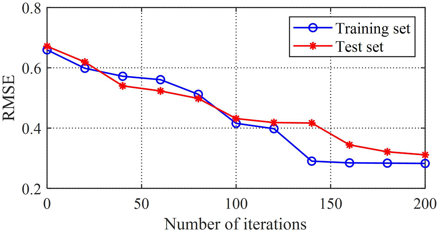
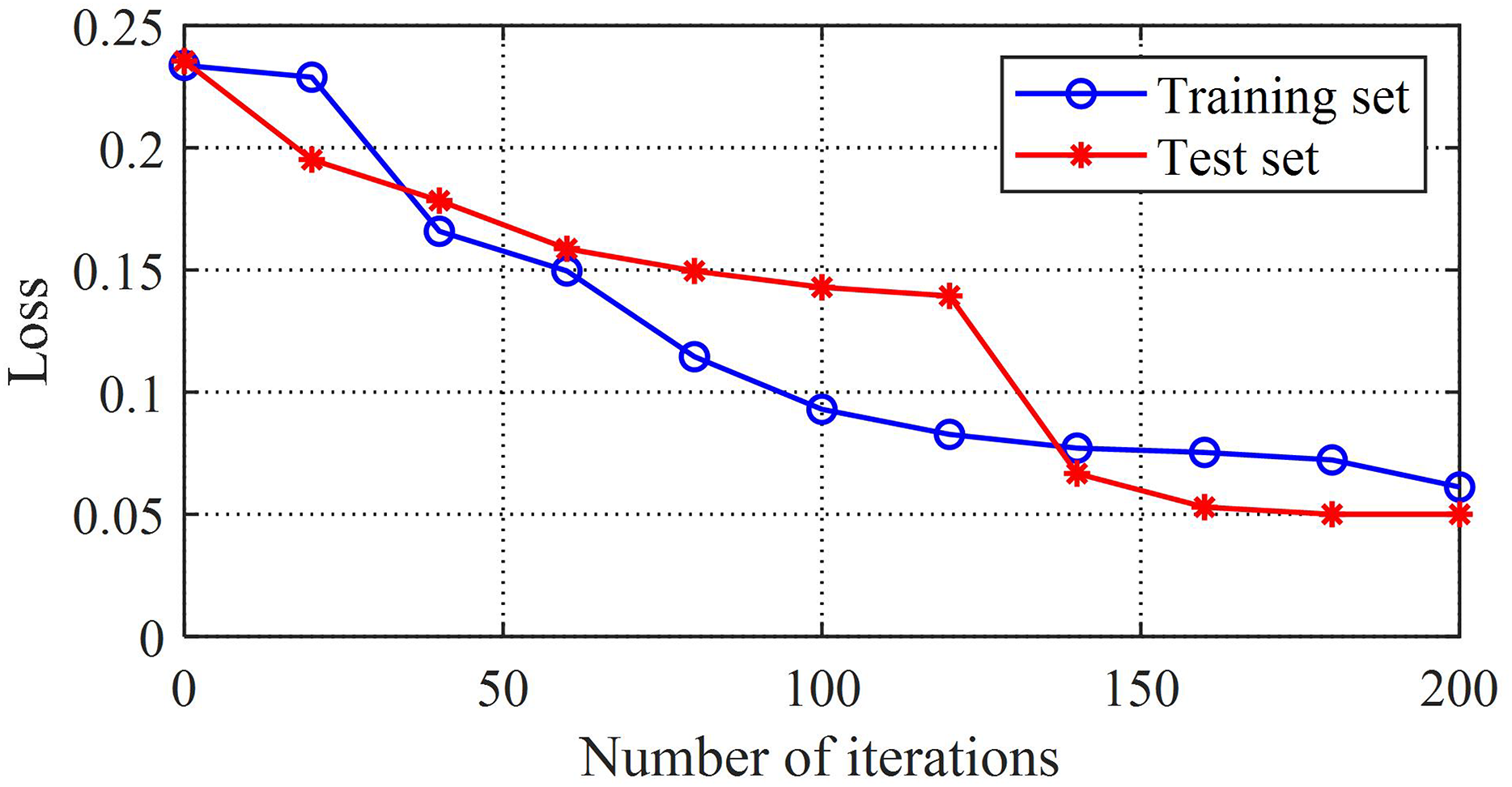
The comparison between the loss value and error value of the training set can reflect the adaptability of the model. The root mean square error curve of the training model in this study is shown in Fig. 5, and the error curve of the training set is shown in Fig. 6. From these two graphs, it can be observed that as the training time increases, the loss and error values first decrease rapidly, then gradually converge and tend to stabilize, and both the loss and error converge to relatively small values. This reflects the good generalization ability and fitting performance of the K-BiLSTM model proposed in this section.
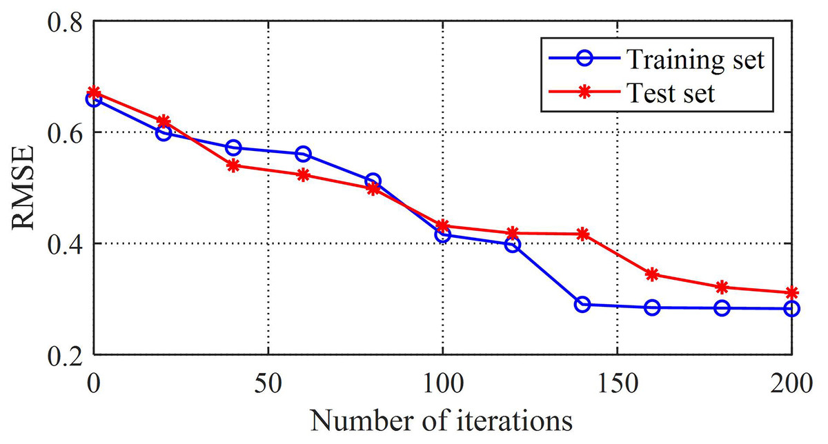
Figure 5: Root mean square error of the training model.
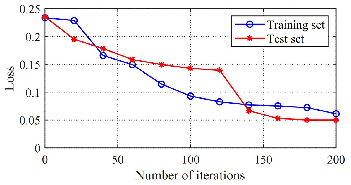
Figure 6: The loss value of the training model.
To further validate the effectiveness of the K-BiLSTM prediction performance proposed in this article, it was compared with the CNN BiLSTM model (Yang & Wang, 2022), BiLSTM Attention (Zhang, Ye & Lai, 2023; Hao et al., 2022), and Complementary Ensemble Empirical Mode Decomposition with Adaptive Noise–Bayesian Optimization–Bidirectional Long Short-Term Memory (CEEMDAN-BO-BiLSTM) (Ying et al., 2023). The RMSE and MAE experimental results of the three methods are shown in Table 3.
| Method | RMSE | MAE |
|---|---|---|
| CNN-BiLSTM | 0.68 | 0.12 |
| BiLSTM Attention | 0.59 | 0.29 |
| CEEMDAN-BO-BiLSTM | 0.71 | 0.17 |
| K-BiLSTM | 0.23 | 0.08 |
Table 3 shows the comparison of the predictive performance of four models under RMSE and MAE indicators. The results show that the K-BiLSTM model proposed in this article performs the best on both indicators, with RMSE of 0.23 and MAE of 0.08, significantly better than CNN BiLSTM, BiLSTM Attention, and CEEMDAN-BO BiLSTM models. This indicates that K-BiLSTM has significant advantages in improving prediction accuracy and stability, and verifies the effectiveness of the model structure that integrates K-means clustering and evidence theory.
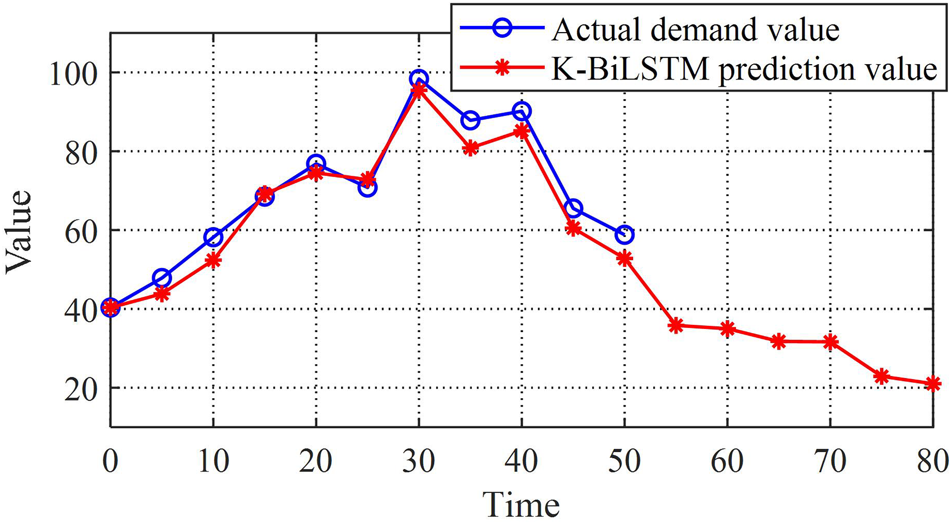
Compare actual sales with K-BiLSTM to further validate the performance of the model. Figure 7 shows the prediction comparison results of the dataset. Through the image, it can be intuitively seen that the actual values are quite close to the predicted values, which preliminarily reflects the good performance of the prediction model established in this chapter. Even for long-term prediction, it can ensure good error control. The final composite predicted value is very close to the actual value, with high prediction accuracy, indicating that the K-BiLSTM model has good predictive ability.
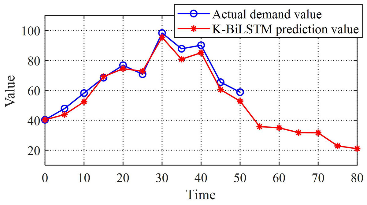
Figure 7: K-BiLSTM model predictions and actual values.
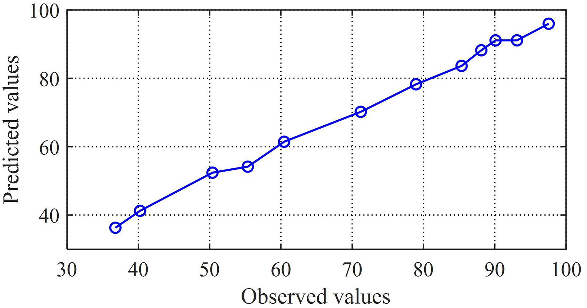
Next, perform a general correlation analysis on the predicted set samples and the true value samples. By plotting the predicted and observed values through a scatter plot, as shown in Fig. 8, it can be observed that there is a clear linear relationship between the two sets of values, and the regression function with the best fit is calculated
(27) where the regression coefficient is 1.002, which is very close to 1. This indicates that the combination prediction value is positively correlated with the observed value, also known as Pearson positive correlation. The close correlation between prediction and reality reflects the good predictive performance of the combination model proposed in this article.
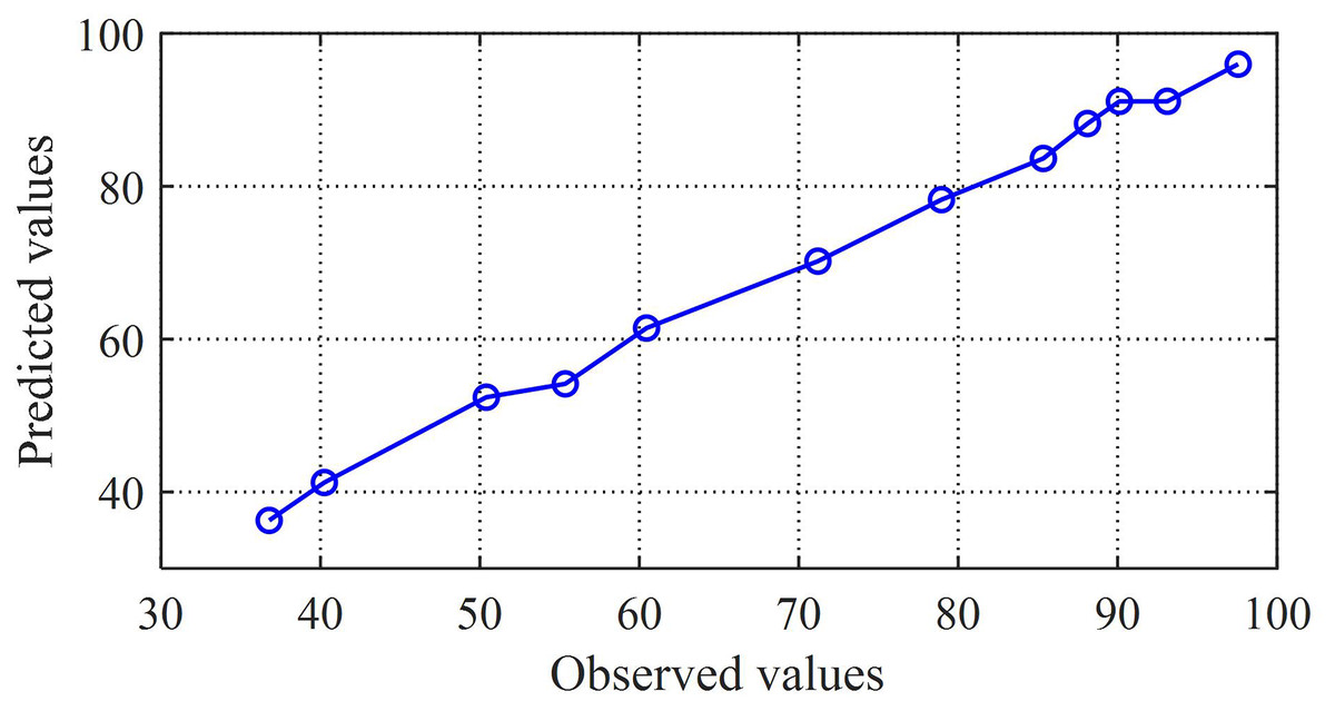
Figure 8: Scatter plot of predicted values and observed values.
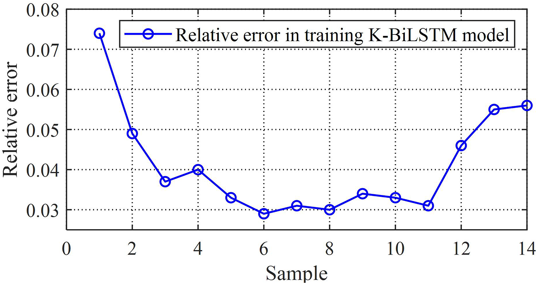
Furthermore, the relative error and absolute error frequency histograms of the K-BiLSTM model are shown in Fig. 9. The occurrence of errors is mainly concentrated in small error events, indicating that the prediction of K-BiLSTM is relatively accurate. The upper limit of relative error does not exceed 8%, indicating that the overall error of the model is not significant, the training effect of the data is good, and the independent remanufacturing supply chain prediction model based on multiple value chains has strong predictive ability.
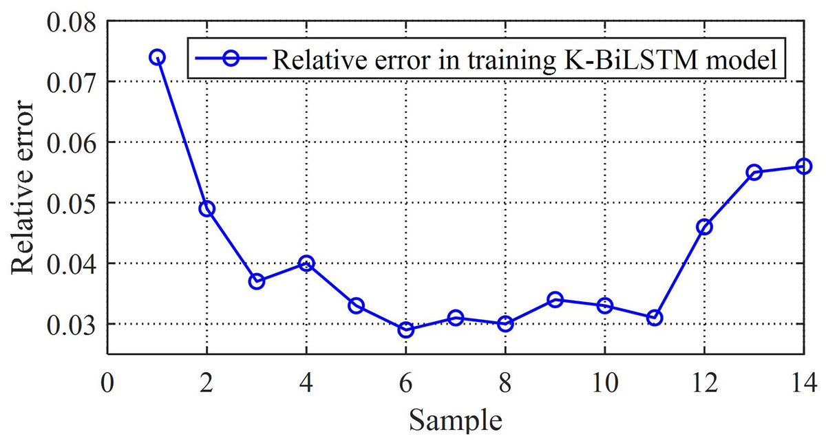
Figure 9: The relative errors of the proposed model.
Furthermore, to better demonstrate the advancement of the proposed algorithm, this article also conducted experimental comparisons with deep learning models, namely Transformer, Graph Convolutional Network–Long Short-Term Memory (GCN-LSTM), and Deep Reinforcement Learning–Bidirectional Long Short-Term Memory (DRL-BiLSTM). The experimental results are shown in Table 4.
| Model | RMSE | MAE | Training time (min) | Parameters (M) |
|---|---|---|---|---|
| K-BiLSTM (Ours) | 0.23 | 0.08 | 45.2 | 2.1 |
| Transformer | 0.41 | 0.19 | 68.7 | 36.5 |
| GCN-LSTM | 0.38 | 0.15 | 52.3 | 4.8 |
| DRL-BiLSTM | 0.35 | 0.12 | 89.1 | 5.2 |
As shown in Table 4, K-BiLSTM achieves the lowest RMSE (0.23) and MAE (0.08), indicating minimal prediction error and the highest accuracy. Simultaneously, the model demonstrates exceptional efficiency, with a training time (45.2 min) significantly lower than that of complex models like Transformer and DRL-BiLSTM, while also having the most compact parameter count (2.1M). This validates that K-BiLSTM achieves an optimal balance between prediction accuracy and computational efficiency, effectively integrating clustering and evidence theory to deliver superior performance with a more concise architecture.
Ablation experimental
To verify the effectiveness and contribution of each component in the proposed K-BiLSTM model, we conducted a series of ablation experiments. The following configurations were tested:
Model 1: Baseline BiLSTM Model: only the BiLSTM model is used, without any clustering or evidence fusion. This serves as the benchmark.
Model 2: K-means + BiLSTM: introduces the K-means clustering layer before the BiLSTM, allowing the model to preprocess and group similar data points for more stable training input.
Model 3: BiLSTM + Dempster-Shafer (DS) Theory: this version applies evidence fusion after BiLSTM outputs to integrate multi-source decision support, but does not perform clustering beforehand.
Model 4: Full K-BiLSTM Model: combines all components—K-means clustering, BiLSTM, and DS evidence theory—into a unified model.
The RMSE and MAE of ablation experimental results are shown in Table 5.
| Method | RMSE | MAE |
|---|---|---|
| Model 1 | 0.56 | 0.25 |
| Model 2 | 0.51 | 0.23 |
| Model 3 | 0.47 | 0.20 |
| Model 4 | 0.23 | 0.08 |
According to the ablation experiment results shown in Table 5, it can be clearly seen the contribution of each component to the model performance:
Starting from Model 1 (using only BiLSTM), its RMSE is 0.56 and MAE is 0.25, which is the lowest baseline model performance. This indicates that although BiLSTM can handle time series data, its prediction accuracy is still limited in the absence of effective data preprocessing and decision fusion mechanisms.
After introducing K-means clustering (Model 2), the RMSE decreased to 0.51 and the MAE decreased to 0.23, indicating that clustering and grouping the input data can help reduce data heterogeneity and noise, making the training process of BiLSTM more stable and slightly improving its predictive ability.
In Model 3 (introducing Dempster Shafer evidence theory), although clustering was not performed, a multi-source evidence fusion mechanism with an output layer was added, resulting in a significant decrease in RMSE to 0.47 and MAE to 0.20. It can be seen that this mechanism plays a significant role in integrating various uncertain information and improving the stability of output decisions.
Finally, in Model 4 (K-BiLSTM complete model), the three key modules of clustering, deep temporal modeling, and evidence fusion were combined, and the RMSE and MAE were reduced to 0.23 and 0.08, respectively, significantly better than other models. This indicates that the combination of each module has a synergistic effect, which can more comprehensively extract features and enhance the model’s generalization ability and robustness.
Conclusion and limitations
This article proposes a K-BiLSTM prediction model that integrates K-means clustering, evidence theory, and BiLSTM to address the issues of multi-agent collaboration and energy awareness prediction in green supply chains. This model combines the advantages of clustering preprocessing, evidence fusion, and deep temporal modeling in structure, and can more accurately capture the nonlinear dynamic characteristics of green behavior evolution process. Through empirical research using a supply chain enterprise in Xi’an as a case study, and comparative experiments with mainstream models such as CNN-BiLSTM, BiLSTM Attention, and CEEMDAN-BO BiLSTM, the results showed that K-BiLSTM performed the best in the root mean square error (RMSE) and mean absolute error (MAE) indicators, reaching 0.23 and 0.08, respectively, significantly better than the comparative models (CNN BiLSTM was 0.68/0.12, BiLSTM Attention was 0.59/0.29, CEEMDAN-BO BiLSTM was 0.71/0.17). The experimental results fully verify the significant advantages of the proposed method in terms of prediction accuracy and model stability.
In future research, we will introduce reinforcement learning mechanisms to enable predictive models to have adaptive optimization capabilities for policy adjustment and behavioral feedback.
Despite its promising results, the study has several limitations that warrant consideration. The model’s performance is contingent on the quality and availability of historical data, which may be inconsistent across supply chain entities, potentially skewing clustering outcomes. The computational demands of BiLSTM and evidence theory integration limit scalability on low-resource systems, restricting real-time application in smaller firms. Additionally, the model was tested on a specific dataset (2023–2024), which may not fully capture long-term trends or diverse regional variations in energy behavior. Future research should address these gaps by incorporating real-time data streams and validating the model across broader geographical contexts.