
Remaining useful life prediction for turbofan engines using an attention-based data-driven deep-learning approach
- Published
- Accepted
- Received
- Academic Editor
- Xiangjie Kong
- Subject Areas
- Algorithms and Analysis of Algorithms, Artificial Intelligence, Data Mining and Machine Learning, Data Science, Neural Networks
- Keywords
- Prognostics and health management (PHM), Aero-engine prognosis, Remaining useful life (RUL), Long short-term memory network (LSTM), Attention mechanism (AM)
- Copyright
- © 2025 Ghoneim et al.
- Licence
- This is an open access article distributed under the terms of the Creative Commons Attribution License, which permits using, remixing, and building upon the work non-commercially, as long as it is properly attributed. For attribution, the original author(s), title, publication source (PeerJ Computer Science) and either DOI or URL of the article must be cited.
- Cite this article
- 2025. Remaining useful life prediction for turbofan engines using an attention-based data-driven deep-learning approach. PeerJ Computer Science 11:e3438 https://doi.org/10.7717/peerj-cs.3438
Abstract
The remaining useful life (RUL) estimate is the fundamental building block of prognostics and health management (PHM), a field that has the potential to increase system safety and save maintenance expenses. Because of their adaptable structures and improved effectiveness in handling nonlinear behaviors, a variety of deep learning (DL) algorithms have surfaced for RUL forecasting. While DL models such as convolutional neural network (CNN) and Long short-term memory (LSTM) have shown promise, they often struggle to capture complex temporal dependencies and to assign appropriate importance to varying sensor features. The LSTM architecture is based on an attention mechanism integrated with an attention block called Dual Attention Block LSTM (DAB-LSTM). Preprocessing the dataset is the first step in the preparatory phase. The piecewise linear degradation approach is then applied to model RUL labels. The addition of the attention mechanism enhances the input features for time steps that are highly correlated with RUL, which helps to improve the network’s feature extraction performance. The adaptive attention method is then included in an LSTM network to effectively collect and evaluate long-term dependencies, use weighted features, and extract feature representations strategies for paying attention that can improve RUL performance by making use of long-term correlations. The Tree-structured Parzen Estimator (TPE) algorithm is used as a hyperparameter optimization method to find the best values for hyperparameters. In the end, weighted characteristics are combined to create RUL values using a fully connected neural network. We have successfully demonstrated the effectiveness of the DAB-LSTM model on the NASA Commercial Modular Aero-Propulsion System Simulation (C-MAPSS) dataset, and the model has demonstrated improved accuracy compared to other competing approaches.
Introduction
Prognostics and health management (PHM) constitutes a fundamental component of intelligent manufacturing systems (Vogl, Weiss & Helu, 2019). PHM represents a computational paradigm that explores the realm of empirical knowledge relevant to the functioning and upkeep of structures, systems, and components (SSCs). The estimation of remaining useful life (RUL) is a critical element of PHM that has garnered considerable attention from the research community in recent years (Cao, 2023). The operational dependability of turbofan engines constitutes an essential metric for evaluating the aviation safety of aircraft (Li et al., 2023). The aero-engine exemplifies a complex aerothermal-mechanical system and constitutes a vital safety-critical component of an aircraft (Gan et al., 2024). The aero-engine constitutes the primary component of the aircraft, responsible for producing a continuous supply of energy.
Being a complex machine, direct variables like design and manufacturing quality may affect how well it works and how long it lasts (Wang et al., 2023). With the ongoing progress in contemporary sensor technologies and the increasing prevalence of automation, the transition from conventional preventive maintenance (PM) to condition-based predictive maintenance (CBPM) signifies a notable advancement in the domain of aviation management (Fan, Li & Chang, 2024). This conventional maintenance approach has the potential to induce superfluous and somewhat redundant maintenance activities, thereby exacerbating the operational expenses of airlines. PM often results in superfluous maintenance activities due to its time-based nature, unnecessarily increasing operational costs and inefficiencies. In contrast, CBPM leveraging real-time sensor data and predictive analytics optimizes maintenance schedules by focusing on actual engine health, as demonstrated by our attention-based deep learning approach for RUL prediction. The shift to CBPM signifies a more effective and forward-thinking approach, improving the dependability and functionality of essential assets while optimizing operational effectiveness (Fan, Li & Chang, 2024). While CBPM for engines has roots in the 90s, driven by early adoption of vibration analysis and basic health monitoring, the paradigm has significantly evolved with contemporary advancements. In contemporary contexts, PHM has been implemented across diverse domains, including healthcare (Kontogiannis & Malakis, 2012; das Chagas Moura et al., 2017), finance (Andersen et al., 2012), and engine systems (Xu, Wang & Xu, 2013; Chen, 2007). The prediction of RUL for an aero-engine aims to estimate the length of time an aero-engine can continue to function prior to experiencing a failure. Precise estimation of RUL can not only minimize the occurrence of unnecessary maintenance interventions and facilitate effective condition-based maintenance but also mitigate the risk of aviation incidents resulting from engine malfunctions.
RUL prediction methods can be classified into three groups: model-based methods, data-driven methods, and hybrid methods (Darwish, 2024a; Wu et al., 2016). The model-based methods are categorized into physics-based methods and knowledge-based methods (Vrignat, Kratz & Avila, 2022). In the physics-oriented approach, a prior understanding of physical principles is essential for the formulation of the physical deterioration model pertaining to the apparatus (Wei, Dong & Chen, 2017; Cui et al., 2019). It works well if the degradation mechanisms are simple to model. Nonetheless, this approach exhibits suboptimal performance when applied to the development of tangible models for various intricate systems (Sun, Zhang & Wang, 2023). Formulating precise physical models that employ iterative methods to align with empirical findings may require an extensive time frame, potentially spanning multiple years. In order to address these obstacles, knowledge-driven approaches entail the creation of a linkage between a monitored operational state of machinery and a previously developed degradation knowledge repository, thereby facilitating the inference of the RUL (Wang et al., 2022). Nevertheless, knowledge repositories that exist in a compromised condition are generally formulated by specialists within a particular domain who depend on recognized principles, verified information, or their individual experiences accumulated over time through the operation of equipment (Djeziri, Benmoussa & Benbouzid, 2019). The precision in estimating RUL may vary according to the proficiency of practitioners within the discipline.
In contrast to model-based methodologies, the data-driven methodology demonstrates superior generalization capabilities and does not necessitate specialized expertise (Darwish, 2024b). Data-driven methodologies elucidate the relationship between sensor data and the extent of system deterioration (Wu et al., 2020). Data-driven techniques demonstrate a significant ability for extrapolation and require limited experiential insight (Fu et al., 2021). Data-driven techniques predict RUL by analyzing degradation patterns taken from past equipment monitoring data (Mitici et al., 2023). Scholars have largely adopted a data-driven approach. This study estimates the RUL of complex systems using a data-driven methodology.
Data-driven methods include machine learning (ML) and deep learning (DL). Machine learning and deep learning methodologies have been extensively implemented across significant domains in practical applications, including but not limited to manufacturing (Alshboul et al., 2024; Arafat, Hossain & Alam, 2024; Wang, Zhu & Zhao, 2024; Elkateb et al., 2024), climate change (Li et al., 2023; Yao et al., 2023; Kumar, 2023; Lou et al., 2023; Shahani et al., 2023), and healthcare (Mbunge & Batani, 2023; Chakraborty et al., 2023; Neto et al., 2024; Wang et al., 2024), among others. This enables computational systems to acquire insights from data without the necessity of direct programming, continuously enhancing their performance. In a broad sense, the potential of machine learning to assimilate information from datasets and perform tasks autonomously is fundamentally transforming our way of life, professional landscape, and engagement with technological systems. Machine learning methodologies possess the ability to leverage vast datasets comprising sensor information, operational metrics, and archival maintenance documentation. As this domain advances, we can foresee increasingly profound implications for our worldwide society. This methodology, which is fundamentally based on data analysis, empowers machine learning models to understand complex interrelations among various elements that influence the state and deterioration of machinery. The estimation of RUL has significantly leveraged conventional machine learning methodologies. For instance, classifiers such as artificial neural network (ANN) (Chinomona et al., 2020), random forest (RF) (Soni et al., 2021), and support vector machines (SVM) (Zhao et al., 2019), among others, are frequently utilized in the context of RUL prediction. Reducing the dimensionality of data and extracting features are essential for machine learning techniques; however, using the wrong features frequently results in weak performance.
The field of deep learning, a prominent area within machine learning, has instigated substantial changes across various dimensions of our lives. It utilizes artificial neural networks that consist of numerous layers to perform data processing in a fashion that mimics the cognitive functions of the human brain. The advancements in deep learning methodologies have been remarkable due to their inherent versatility. These deep learning techniques obviate the necessity for feature engineering, as they possess the capability to autonomously derive feature representations. Deep learning employs a forward training process alongside reverse fine-tuning of data by developing a multilayered neural network, thereby thoroughly exploring the latent features within the data to derive precise predictive outcomes. The prediction of RUL can be essentially classified as a time series regression issue. The deep learning models demonstrated efficacy in identifying time-related features from historical observational data. The methodologies for predicting RUL can be executed utilizing recurrent neural networks (RNNs) (Costa & Sánchez, 2022), LSTM architectures (Arunan et al., 2024; Boujamza & Elhaq, 2022; Cheng et al., 2023), gated recurrent units (GRUs) architectures (Duan et al., 2021), convolutional neural networks (CNNs) (Mo et al., 2021; Li et al., 2022), gray neural networks (Chen et al., 2022), and transfer learning techniques (Siahpour, Li & Lee, 2022), among others.
Despite remarkable advances in attention-based RUL prediction models, most existing approaches still face critical challenges in effectively capturing the joint influence of temporal and sensor-level dependencies. These methods often treat temporal and contextual modeling as separate components, which limits their capacity to represent complex degradation dynamics in aero-engines. Additionally, many frameworks lack interpretability, offering limited insight into which features, or time steps most strongly influence predictions. To address these issues, this study introduces the Dual Attention Block LSTM (DAB-LSTM) model, which integrates a dual-phase attention mechanism capable of simultaneously modeling temporal and feature-wise dependencies. This architecture enhances both predictive performance and interpretability, representing a distinct contribution beyond existing single-attention or hybrid models. DAB-LSTM is a new hybrid data-driven DL model for RUL prediction of aero-engines. The DAB-LSTM incorporates dual attention mechanisms. We implement the Attention Block founded on the dot product attention mechanism to facilitate the LSTM in forecasting an accurate RUL. To augment the model’s predictive efficacy and to more precisely depict the long-term interrelations among states, it can dynamically assign differing attention weights to various states; thus, we incorporate the adaptive attention mechanism for the output of the LSTM. The major contributions of this article are listed as follows:
-
We propose a dual-phase attention framework that progressively integrates temporal attention with sensor-specific variable attention. This design enables simultaneous modeling of temporal dependencies and feature-wise relationships, distinguishing our method from existing approaches that handle these aspects independently.
-
A hybrid deep learning model, termed DAB-LSTM, is developed by embedding both an attention block and an adaptive attention mechanism into the LSTM architecture. This integration enhances the model’s capacity to capture long-term dependencies and focus selectively on the most informative features, leading to improved accuracy and stability in RUL prediction.
-
The proposed framework introduces a joint adaptive learning mechanism that dynamically balances the contributions of temporal and sensor-level attention within a unified architecture. Unlike conventional single-attention or sequential designs, this dual-attention synergy improves the interpretability of the model by revealing the most influential sensors and time intervals contributing to engine degradation, while simultaneously enhancing predictive performance across multiple evaluation metrics.
-
A comprehensive set of experiments and ablation studies on the NASA C-MAPSS dataset (Saxena et al., 2008), demonstrates the effectiveness of the proposed approach. The DAB-LSTM consistently outperforms benchmark models in terms of RMSE and Score metrics, validating the framework’s robustness, generalization, and practical applicability in aero-engine prognostics.
The remainder of this article is organized as follows: ‘Related Literature’ covers related work; ‘The Proposed Method’ introduces the proposed attention-based RUL prediction model; ‘Experimental Settings’ outlines experimental settings; ‘Experimental Results and Analysis’ analyzes results; and ‘Conclusions’ concludes the study.
Related literature
The convolutional neural network architecture is extensively implemented in remaining useful life forecasting. A stacked deep convolutional neural network (stacked DCNN) framework was introduced by Solis-Martin, Galán-Páez & Borrego-Diaz (2021), which employs a dual-layered configuration of deep convolutional neural networks to effectively manage low-dimensional feature extraction and RUL prediction. Wang et al. (2021) introduced the spatiotemporal non-negative projected convolutional network (SNPCN) framework for identifying degradation patterns in neighboring matrices through the utilization of a three-dimensional convolutional neural network (3DCNN). Subsequently, the authors employed the PRONOSTIA platform to assess the effectiveness of this methodology.
Chen et al. (2022) employed convolutional kernels of varying dimensions to construct a deep convolutional neural network (DCNN) aimed at feature extraction and forecasting the RUL of engines. The most popular deep learning architecture that is used is the RNN model, and a large body of research has been done on RNN-based prediction methods (Zhao, Zhang & Wang, 2022; Catelani et al., 2021), which are frequently utilized for RUL prediction. Because of their efficiency in managing time-series data, RNN-based models have been extensively utilized for RUL prediction. Lin et al. (2022) developed a sophisticated deep LSTM network designed to extract temporal correlations from sensor data gathered over an extended timeframe. This architecture enables the prediction network to effectively preserve significant degradation information. In order to capture feature information from multi-scale temporal series, they adjust the sequence length. This adjustment facilitates the network in accessing comprehensive information and acquiring essential time-related insights.
Liu, Song & Zhou (2022) devised a prediction model utilizing LSTM networks for forecasting the remaining useful life of engines and diagnosing faults. In a similar vein, Chen et al. (2022) established a data-mining framework that integrates a multilayer LSTM architecture along with a conventional feedforward layer, enabling the prediction of RUL across diverse operational conditions, fault scenarios, and degradation models. Hu et al. (2021) proposed deep bidirectional recurrent neural networks (DBRNN) ensemble comprising three distinct RNN architectures to extract latent degradation patterns from sensor data. Bidirectional traditional RNN (Bi-TRNN) processes sequential data with simple recurrent units, capturing short-term dependencies in adjacent time steps. Bidirectional long short-term memory (Bi-LSTM) uses input, forget, and output gates to mitigate vanishing gradients, excelling at modeling long-range dependencies in degradation sequences. Bidirectional gated recurrent unit (Bi-GRU) employs reset and update gates (simplified vs. LSTM) to balance computational efficiency and intermediate-term dependency learning. The DBRNN model leverages both forward and backward data sequences to improve its ability to perceive data. Additionally, the integration of multiple networks enhances the overall prediction accuracy and generalization performance by creating an ensemble model.
Li et al. (2021) proposed a method that integrates the attention mechanism and LSTM architecture for predicting the RUL of rolling bearings. Cao (2023) proposed the DCNN-BiLSTM network. The utilization of the DCNN and the Bi-LSTM allows this network to take advantage of their respective abilities in feature extraction and bidirectional time-series feature capturing. The K-means algorithm is utilized to unveil prospective operational patterns within the data, which subsequently results in the achievement of a remarkably efficient data preprocessing technique. To expedite the training process of an LSTM-based method, Chen et al. (2019) devised an alternative method using GRU for predicting the RUL of aero-engines.
Zhang et al. (2022) applied a Bi-GRU, which incorporates a temporal self-attention mechanism for predicting the RUL. This method employs a self-learning weight that is determined based on the level of importance, thereby facilitating accurate and efficient RUL prediction. A temporal attention mechanism was implemented to assign weights to input features. Subsequently, the Bi-GRU network was employed to extract features that are closely associated with time. The temporal attention mechanism aids the Bi-GRU network in focusing on time steps that are highly pertinent to RUL and thereby enhances the accuracy of RUL prediction. Que, Jin & Xu (2021) proposed a model for predicting the RUL of bearings using a GRU-based approach. The model integrates an attention mechanism based on dynamic time warping and utilizes a Bayesian layer to establish a mapping between features and RUL through regression.
Despite the substantial advancements in RUL prediction using deep learning techniques, existing models still encounter challenges in effectively capturing long-term temporal dependencies and selectively focusing on the most informative features. Most existing methods either rely on single attention mechanisms or treat attention and temporal modeling independently, limiting their ability to exploit complex temporal and contextual interactions within the sensor data. Moreover, many models lack architectural flexibility to integrate multi-scale feature representations, which is critical for modeling the non-linear degradation behaviors typical in turbofan engines. To address these gaps, we propose DAB-LSTM, a novel hybrid architecture that integrates a dual-phase attention framework to jointly optimize temporal and sensor-specific feature importance, coupled with an adaptive attention mechanism that dynamically adjusts weights based on real-time contextual cues. By unifying these components, our model achieves superior generalization across diverse operational scenarios, as demonstrated by significant improvements in RMSE and score metrics compared to state-of-the-art methods.
The proposed method
The estimation of the remaining useful life for an aero-engine is regarded as a time series regression task. Data obtained from various sensors is used as input to estimate the remaining lifespan of the system. The DAB-LSTM model is based on LSTM, an attention block, and an adaptive attention mechanism. It is specifically constructed to capture the nonlinear correlation between the monitored data and the RUL.
DAB-LSTM framework materials
LSTM layer
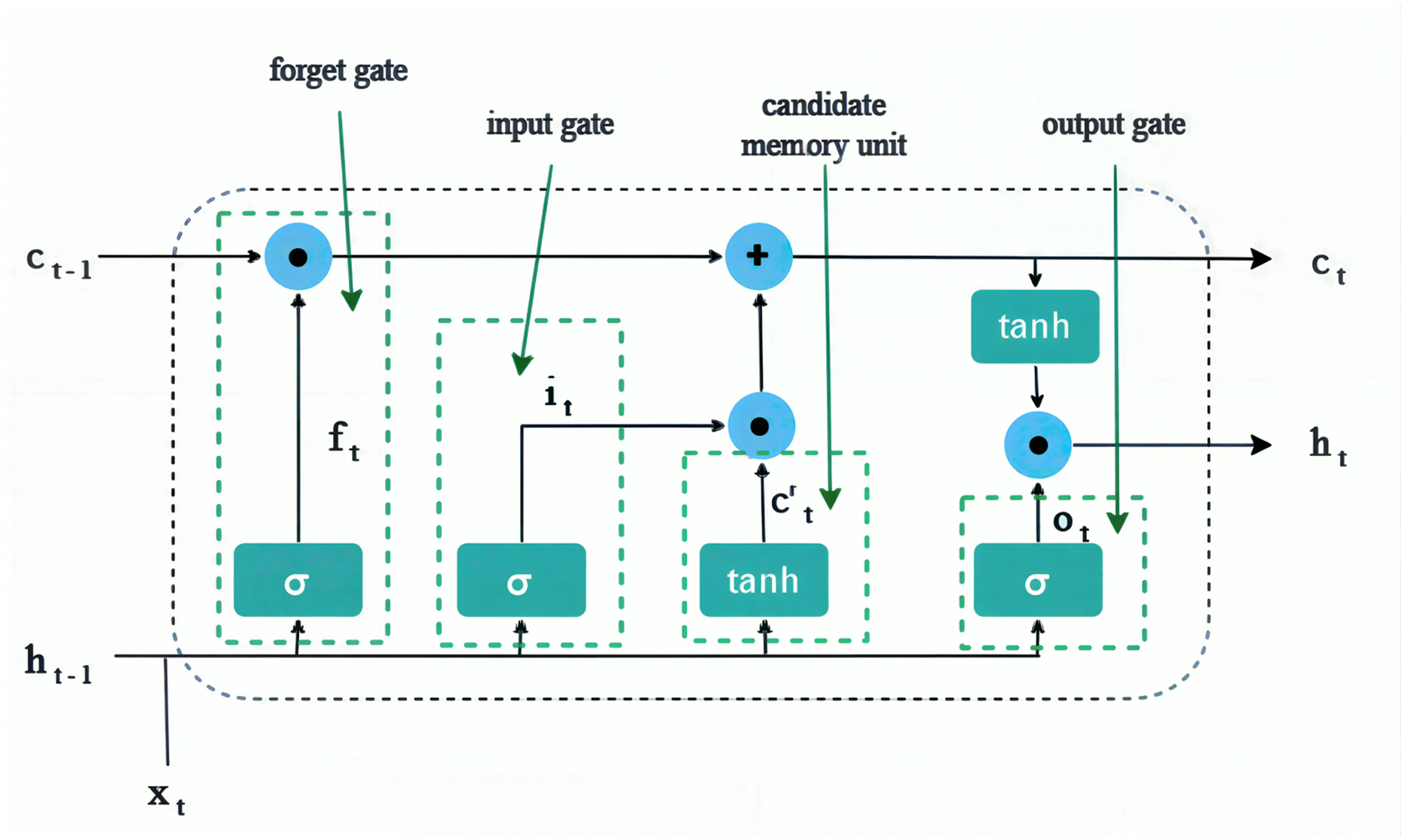
LSTM embodies a specific type of RNN architecture designed to address the vanishing gradient problem, a common obstacle encountered in the training of conventional RNNs. The phenomenon of the vanishing gradient emerges due to the propagation of gradients across multiple temporal steps throughout the training procedure, thereby presenting a significant obstacle for the neural network in its ability to learn long-range dependencies. LSTMs are excellent at capturing long-term dependencies in time series data. LSTMs can handle a wide range of time series patterns, including nonlinear trends, seasonality, and noise. They can adapt to changes in the underlying data-generating process, making them robust to real-world data. LSTM networks feature a sophisticated memory cell architecture that permits the retention of information throughout lengthy sequences, making them particularly suitable for tasks associated with time series data, such as the estimation of remaining useful life in aero-engines. As illustrated in Fig. 1, the architecture of LSTM includes gates, specifically the forget gate , input gate , and output gate which are implemented to address the issue of gradient vanishing, and their values are calculated by Eqs. (1), (2), and (3) respectively (Graves, 2012).
(1)
(2)
(3) where indicates the sigmoid function, t indicates the time sample, indicates the input feature at time t, indicates the output hidden state from the previous time sample, These are parameters that are optimized during the training process.
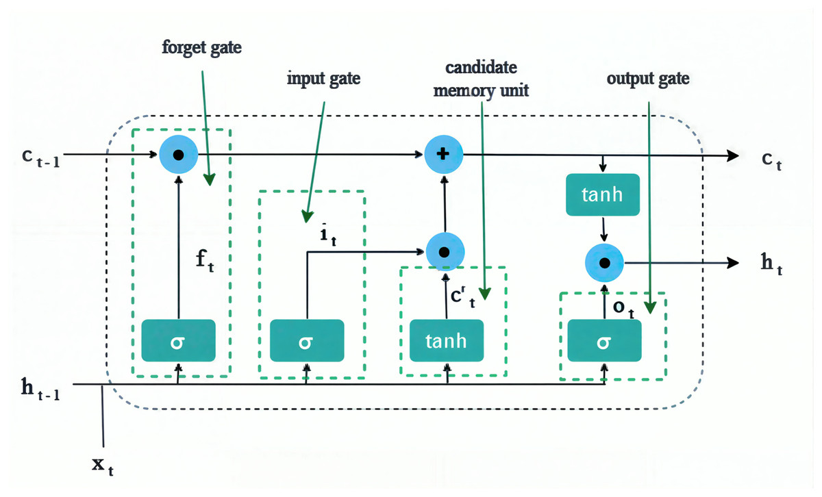
Figure 1: LSTM cell.
The forget gate determines which information from the previous cell state should be discarded. Then, the input gate decides which new information should be stored in the cell state. Then, the output gate controls the information that is passed on to the next step and used for prediction. Subsequently, the candidate memory component, which pertains to the information that may be incorporated into the cell state at a specific temporal point, is determined. In the process of computing the cell state modification, an LSTM unit participates in the assessment of a candidate memory update . This particular calculation serves to denote the new information that can potentially be retained within the cell state at a given time step t. calculated by Eq. (4)
(4)
(5)
(6) where are parameters that are optimized during the training process. Then, calculate the that indicates to unit state at time t. it is calculated by Eq. (5). Then calculate the that indicates the hidden state at time t. ht calculated by Eq. (6).
Adaptive attention mechanism
The conventional approach to assigning attention weights is predicated on the resemblance between query and key vectors. Conversely, the adaptive attention mechanism incorporates both contextual information and the input data, thereby enabling the model to modify the attention weights dynamically and selectively concentrate on varying segments of the input sequence. The adaptive attention mechanism is implemented following the LSTM layer. LSTM layers excel at identifying the sequential dependencies inherent in input sequences. However, they may face challenges in capturing long-range relationships or adequately concentrating on critical portions of the input sequence. By incorporating an adaptive attention mechanism after an LSTM layer, the model gains the ability to dynamically allocate its focus to different segments of the input sequence, thus enhancing its understanding of the contextual information and its efficacy in extracting relevant data. The adaptive attention mechanism’s output is computed using the calculations shown below (Vaswani et al., 2017):
(7)
(8)
(9)
(10) where , and are trainable parameters, stands for the input tensor, and donates the number of samples. Also, the adaptive attention mechanism facilitates the model’s ability to selectively integrate data from various segments of the input sequence, considering their pertinence to the present context. This process of selective information fusion empowers the model to concentrate on the most informative components of the sequence, disregarding any irrelevant or noisy information. Consequently, this leads to more accurate RUL predictions.
Attention block
The attention block (AB) is a constituent of neural network architecture that amalgamates the notions of attention mechanisms and residual connections. The AB is responsible for capturing long-range dependencies, and it is of utmost importance to pay attention to the pertinent sections of the input sequence, so it is useful to use it in time-series problems to capture long-range dependencies. The constructed AB consists of a convolutional layer, dropout, attention mechanism, and fully connected layer. The convolutional layer assumes an essential function in time series issues by allowing the extraction of significant characteristics, capturing localized patterns, and facilitating efficient and effective acquisition of knowledge from sequential data. Dropout is integrated to prevent overfitting by randomly eliminating a fraction of the neurons during training. An attention block constitutes a formidable instrument within the realm of deep learning, enabling a model to concentrate on particular segments of its input by ascribing differing levels of significance to various components. This process, which draws inspiration from the concept of human attention, markedly amplifies the model’s capacity to discern pertinent information and augments its overall efficacy.
The attention module employed in the present research constitutes a component of neural network architecture that integrates the principles of attention mechanisms alongside residual connections. The attention block is crucial for identifying long-range dependencies, and it is essential to focus on the relevant segments of the input sequence. Consequently, its application in time-series analysis proves beneficial for addressing long-range dependencies. The designed attention block comprises a convolutional layer, dropout, attention mechanism, and a fully connected layer. The convolutional layer plays a pivotal role in time series analysis by enabling the extraction of critical features, identifying localized trends, and promoting the efficient and effective acquisition of insights from sequential data. The dropout technique is incorporated to mitigate overfitting by randomly deactivating a portion of the neurons during the training process. A model that finds connections between distant components within a given sequence is made possible by the incorporation of the scaled dot-product attention mechanism into the attention block. This is achieved by computing attention scores, which are established by assessing the similarity between the query and key vectors. Through this process, the model gains the capacity to focus on pertinent data over the course of the input sequence, leading to a better understanding of long-range dependencies. To convert the attention mechanism’s output into a proper representation that can be processed further, the dense layer plays a critical role.
DAB-LSTM framework
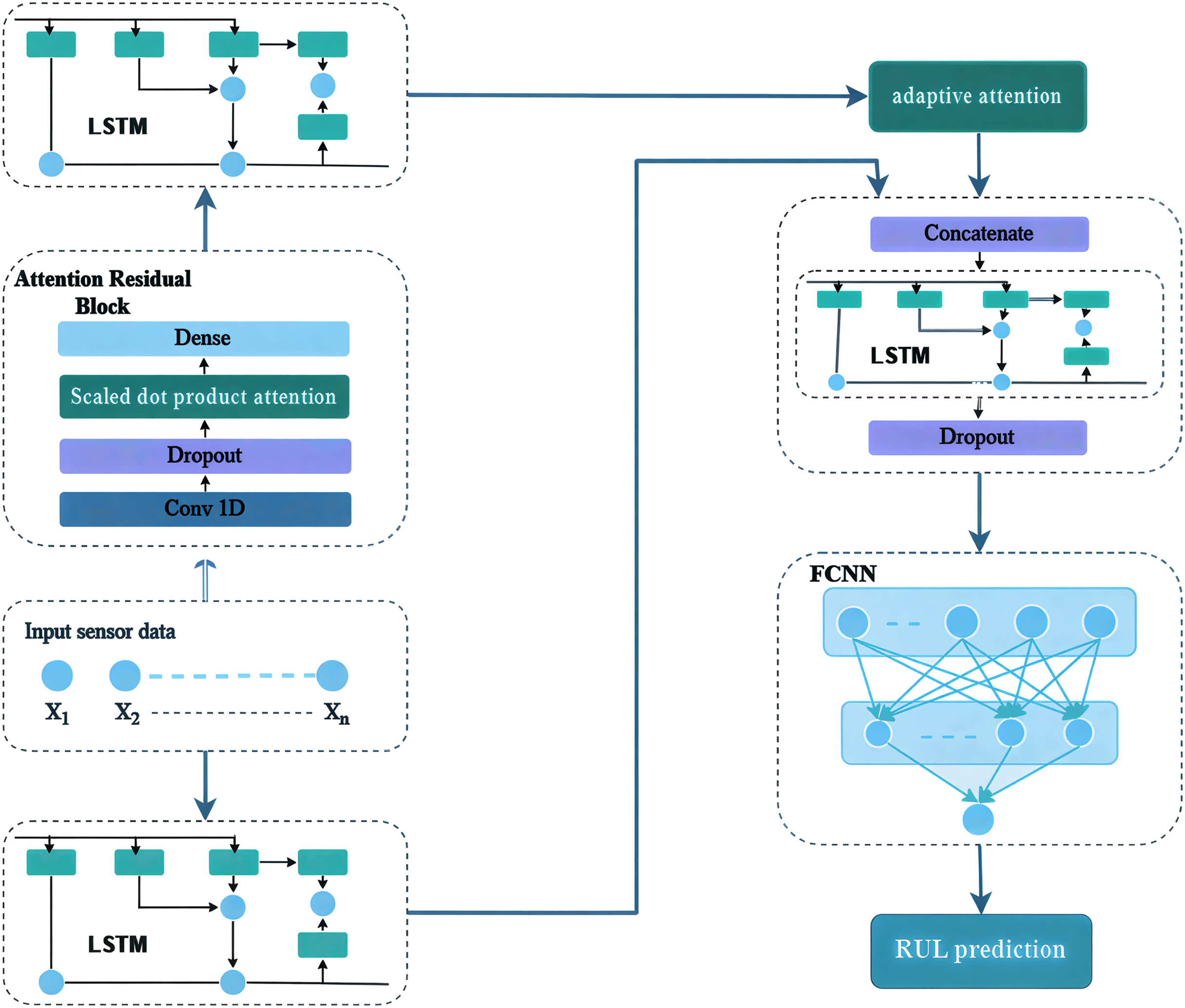
The evaluation of the remaining useful life of an aero-engine is classified as a supervised regression problem, relying on data acquired from diverse sensors for the purpose of training and assessing various deep learning models. In this study, we introduce a novel hybrid data-driven deep learning architecture that integrates long-term memory, an adaptive attention mechanism, and an attention block, termed DAB-LSTM, for RUL estimation of aero-engines. This architecture processes the input sensor data through two concurrent pathways. The initial pathway incorporates an LSTM to capture temporal dynamics within the input data. Simultaneously, the secondary parallel pathway features an attention residual block designed to extract the most pertinent characteristics, which are then directed towards a scaled dot-product attention mechanism to emphasize the most informative features. Subsequently, the result from the initial pathway is utilized as an input for an adaptive attention mechanism, which enhances the selection of salient features while disregarding those of lesser significance. The outcomes from both pathways are merged and supplied as input to an LSTM network, facilitating a more effective assimilation of temporal information. The resultant output from this LSTM is then directed to a fully connected layer to execute the prediction phase. Ultimately, Algorithm 1 outlines the pseudocode for the proposed framework, while Fig. 2 illustrates the schematic representation of its architecture.
| Input: Input data (D), batch size (Bs), maximum epoch (T), and number of trails (R) |
| Output: loss ( ), RMSE |
| 1: Conducting the preprocessing step |
| /* Create the proposed DAB-LSTM model */ |
| 2: Input: Construct an input layer to receive the input data |
| /* First Parallel Path*/ |
| 3: Path1: Create LSTM layer with 256 units and Tanh activation function to take the data from input layer |
| /* Second Parallel Path*/ |
| 4: Path2: Create Conv-1D layer with 32 filters and kernel size of 2 to take the data from input layer |
| 5: Path2: Add Dropout layer with a dropout rate of 0.6 to Path2 |
| 6: Path2: Add Scaled dot product attention mechanism to Path2 |
| 7: Path2: Add a dense layer with 32 nodes and ReLU activation function to Path2 |
| 8: Path2: Add an LSTM layer with 128 units and Tanh activation function to Path2 |
| 9: Path2: Add an adaptive attention with 32 units to Path2 |
| /* Concatenation stage */ |
| 10: x: Concatenate ([Path1, Path2]) |
| 11: x: Add an LSTM layer with 64 units and Tanh activation function to x |
| 12: x: Add Dropout layer with a dropout rate of 0.6 to x |
| /* Prediction Block */ |
| 13: x: Add a dense layer with 1 nodes to x |
| /* Optimization process using The TPE algorithm */ |
| 14: r = 0, Current trail |
| 15: while r < R |
| 16: generate hyperparameters using TPE |
| 17: N = Size(D)/Bs |
| 18: , Current epoch |
| 19: while |
| 20: , the current batch size |
| 21: while |
| 22: Compute the Score function using the batch |
| Update the weights based on the Adam to optimize the score function |
| 23: |
| 24: end while |
| 25: |
| 26: end while |
| 27: |
| 28: end while |
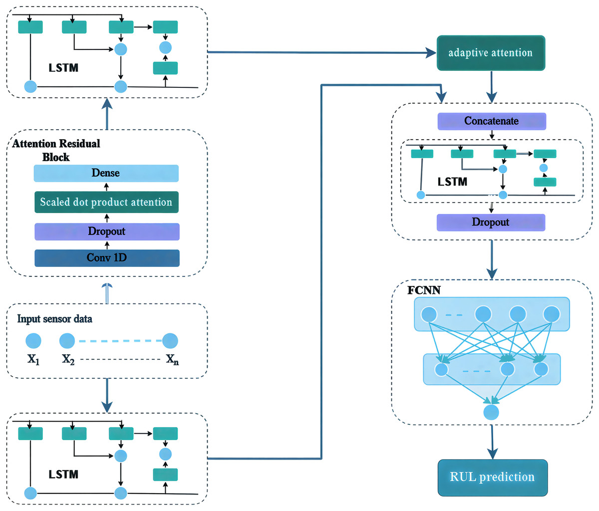
Figure 2: DAB-LSTM framework.
As delineated in Algorithm 1, the proposed framework assimilates the input dataset for preprocessing to eliminate various complications, such as outliers and irrelevant or redundant features. Subsequently, the input layer processes this data and channels it through two concurrent pathways. The initial pathway incorporates an LSTM comprising 256 neurons coupled with a Tanh activation function to capture temporal patterns from the input data. In parallel, the secondary pathway integrates an attention mechanism aimed at identifying the most salient features and focusing on the most informative attributes. The attention block processes the input sequences and subsequently transmits them to a convolutional layer comprising 32 filters, each with a kernel size of 2, to produce a set of feature maps that facilitate the extraction of the most relevant characteristics from the input data. These feature maps are then passed through a dropout layer with a dropout rate of 0.6, intended to reduce the number of trainable parameters in order to mitigate overfitting and enhance the generalization capability of the model. The resulting data is directed at a scaled dot-product attention mechanism, which further emphasizes the most salient features. These features are then forwarded to a fully connected (FC) layer comprising 32 neurons with a ReLU activation function, used to focus on the most impactful features. Subsequently, an LSTM layer comprising 128 neurons with Tanh activation functions processes the output from the attention block, thereby enhancing the extraction of temporal information. This temporal data is then passed through an adaptive attention mechanism to focus on the most critical features.
The results from the aforementioned two pathways are amalgamated through a concatenation layer and subsequently directed to an additional LSTM layer comprising 64 units, utilizing the Tanh activation function. This is followed by a dropout layer with a rate of 0.6, representing a further effort to enhance the efficacy and generalization capability of the proposed model. Finally, the output from this layer is passed to a fully connected layer with a single neuron, which is responsible for forecasting the remaining useful life of the aero-engines.
Experimental settings
The implementation was carried out using Python 3.8 as the primary development environment, with all experiments conducted on the Google Colab cloud platform. The computational workload was handled by a virtual machine configured with 2 CPU cores, 12 GB of DDR4 RAM, and 70 GB of NVMe storage, operating on Ubuntu 20.04 LTS. This cloud-based setup ensured reproducible experimental conditions and maintained hardware consistency across all trials.
C-MAPSS dataset
The NASA C-MAPSS aircraft engine degradation dataset was used in this article as a commonly used benchmark dataset to assess the RUL prediction methods (Saxena et al., 2008). This dataset simulates the actual degradation of the turbofan engine. The C-MAPSS platform was used to simulate the performance, degradation, and failure modes of turbofan engines under realistic operating conditions and collect degradation data. Engine units deteriorate over time as a result of repeated cycles under various operational circumstances and failure modes. The C-MAPSS dataset has four sub-datasets. The four sub-datasets are FD001, FD002, FD003, and FD004. Each subset of data consists of two distinct sets: a training set and a test set. Both sets contain valuable information about the trajectory number of the data, the operational conditions under which it was collected, and the specific failure modes observed. The description of the C-MAPSS dataset is explained in Table 1. Engine sensor testing results under one operating condition are represented by FD001 and FD003, while engine sensor testing results under six operation circumstances are represented by FD002 and FD004. Each sample in the dataset comprises 26 features such as the serial number, degradation cycle, three operational conditions, and 21 values from the sensor data. The details of the 21 sensors are listed in Table 2, and for more additional information is provided in Saxena et al. (2008). The dataset is publicly available on Kaggle (https://www.kaggle.com/datasets/behrad3d/nasa-cmaps).
| Dataset | C-MAPSS | |||
|---|---|---|---|---|
| FD001 | FD002 | FD003 | FD004 | |
| Train units | 100 | 260 | 100 | 249 |
| Test units | 100 | 259 | 100 | 248 |
| Operation condition | 1 | 6 | 1 | 6 |
| Fault mode | 1 | 1 | 2 | 2 |
| Min cycles | 128 | 128 | 145 | 128 |
| Max cycles | 362 | 378 | 525 | 543 |
| Avg cycle | 206 | 207 | 247 | 246 |
| Sensor number | Description | Symbol | Units |
|---|---|---|---|
| Sensor_1 | Total temperature at fan inlet | T2 | °R |
| Sensor_2 | Total temperature at LPC outlet | T24 | °R |
| Sensor_3 | Total temperature at HPC outlet | T30 | °R |
| Sensor_4 | Total temperature at LPT outlet | T50 | °R |
| Sensor_5 | Pressure at fan inlet | P2 | Psia |
| Sensor_6 | Total pressure in bypass-duct | P15 | Psia |
| Sensor_7 | Total pressure at HPC outlet | P13 | Psia |
| Sensor_8 | Physical fan speed | Nf | Rpm |
| Sensor_9 | Static pressure at HPC outlet | Nc | Rpm |
| Sensor_10 | Engine pressure ratio (P50/P2) | Epr | ––– |
| Sensor_11 | Static pressure at HPC outlet | Ps30 | Psia |
| Sensor_12 | Ratio of fuel flow to Ps30 | Phi | pps/psi |
| Sensor_13 | Corrected fan speed | NRf | Rpm |
| Sensor_14 | Corrected core speed | NRc | Rpm |
| Sensor_15 | Bypass ratio | BPR | ––– |
| Sensor_16 | Burner fuel–air ratio | farB | ––– |
| Sensor_17 | Bleed enthalpy | htBleed | ––– |
| Sensor_18 | Demanded fan speed | Nf_dmd | rpm |
| Sensor_19 | Demanded corrected fan speed | PCNfR_dmd | rpm |
| Sensor_20 | HPT coolant bleed | W31 | lbm/s |
| Sensor_21 | LPT coolant bleed | W32 | lbm/s |
Data preprocessing
Sensor selection
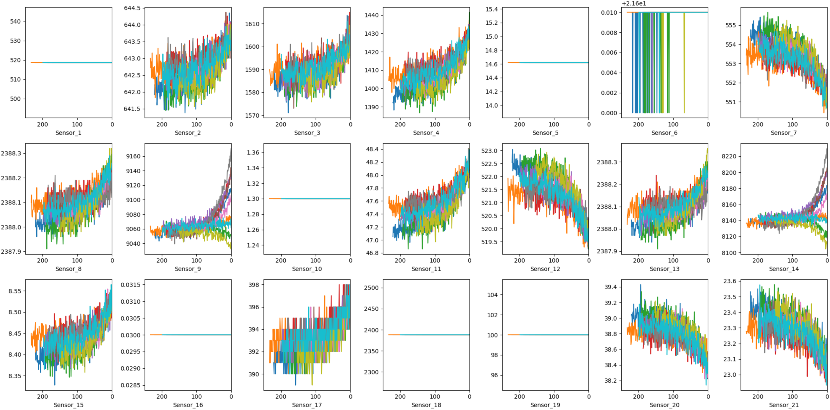
For the purpose of building the model, only sensor signals that demonstrate a clear upward or downward trend should be selected. Sensors that either show erratic patterns or remain constant over time do not contribute meaningful information to the degradation process and can be excluded as input features. Figure 3 displays the readings from all 21 sensors obtained from the engines in the FD001 training set, where the x-axis represents the RUL value and the y-axis represents the sensor readings. Certain sensor readings—specifically from sensors 1, 5, 6, 10, 16, 18, and 19 remain relatively constant and will not be used for RUL estimation. In contrast, sensors 2, 3, 4, 7, 8, 9, 11, 12, 13, 14, 15, 17, and 21 exhibit distinct patterns and are therefore selected as input features.
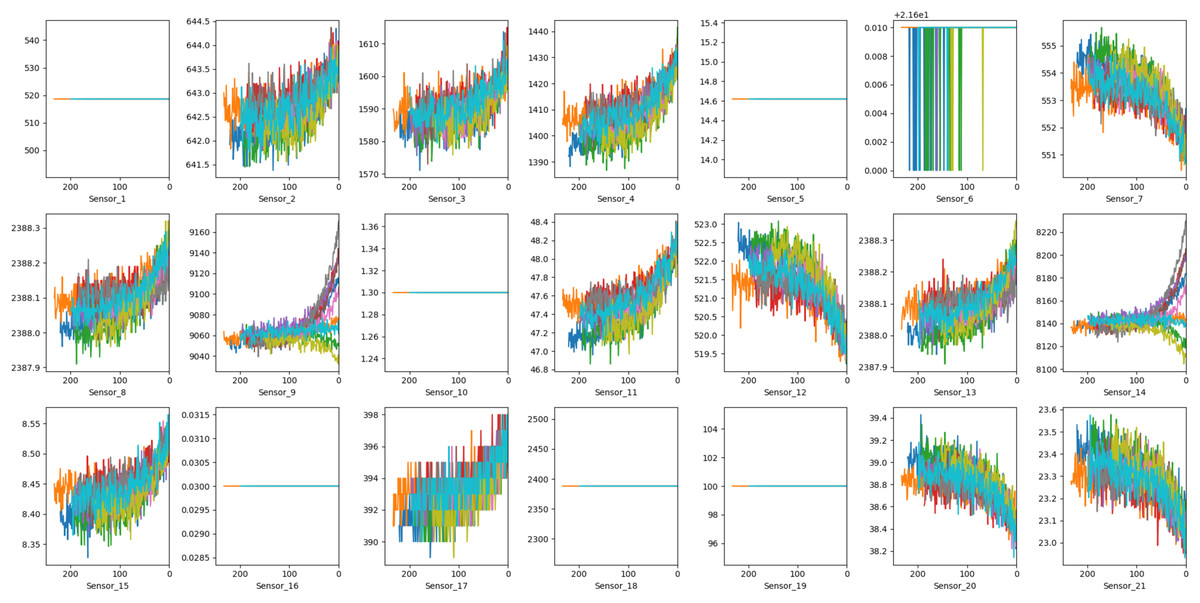
Figure 3: Visualize the information collected by 21 sensors from the FD001 training set.
Data normalization
The performance of deep learning models during training is adversely affected by features with varying scales in the C-MAPSS dataset. Normalizing such features is, therefore, necessary to eliminate any potential biases and distortions and improve the accuracy of the deep learning models. Z-score normalization has been widely used because of its simplicity and effectiveness, although several normalization techniques, including robust scaling normalization, min-max scaling, log scaling normalization, and decimal scaling normalization, have been proposed in the literature to carry out this process (Singh & Singh, 2020; Zheng et al., 2017). In order to mitigate the impact of outliers and dominant features, our study adopts this approach when normalizing the C-MAPSS dataset. According to the following definition, the z-score normalization method’s mathematical model is:
(11) where refer to the original value of the feature number j of the sample number i, the meaning of the feature number j, and the standard deviation of the feature number j.
Sliding time window
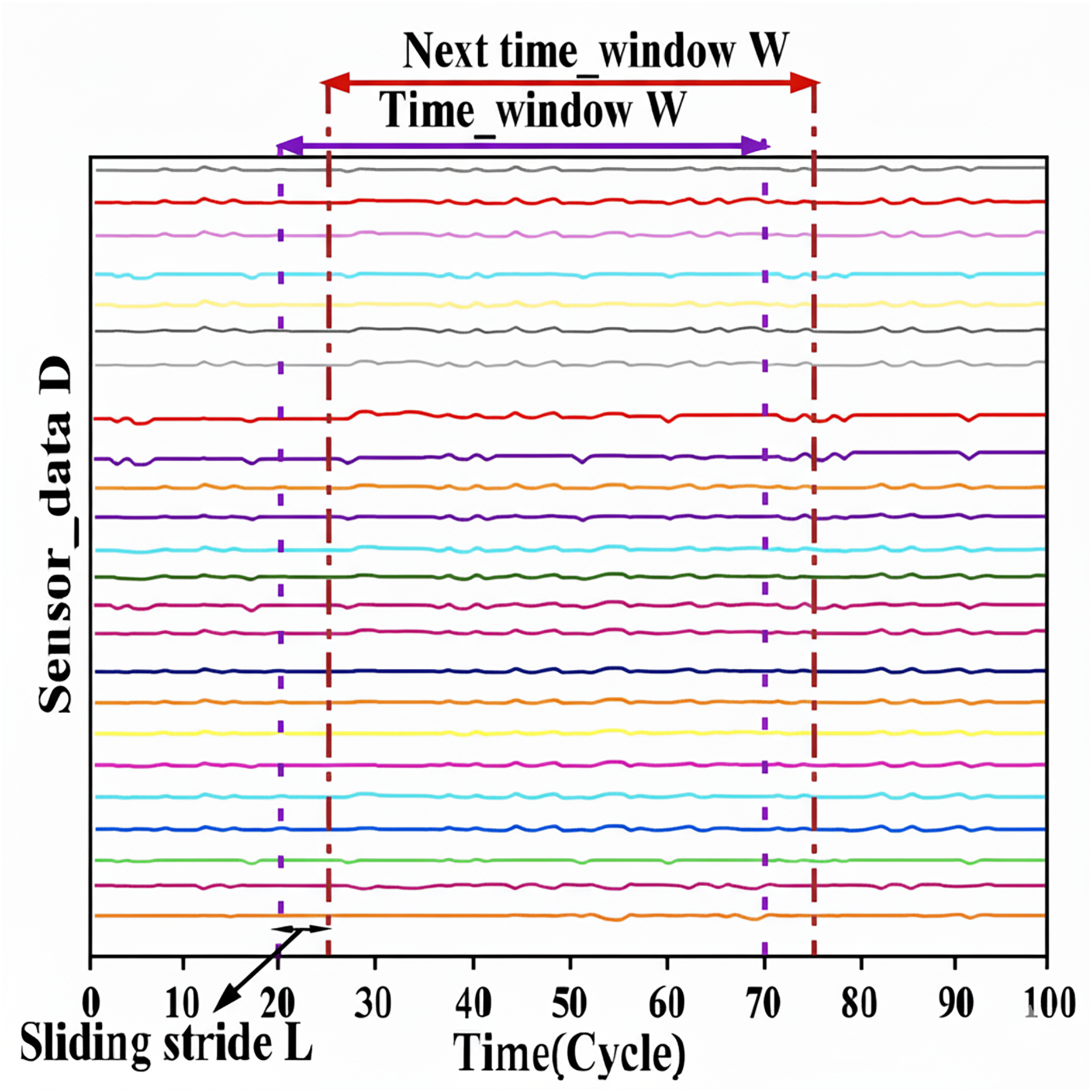
Given the significant correlation between data and temporal variables, it is imperative to choose an appropriate temporal window to accurately capture this interdependent relationship, which is crucial for analyzing time series data. The sliding time window is a technique for data augmentation used in time series analysis that utilizes fixed-size windows to capture and examine the interconnections within these series. The sliding window methodology partitions the normalized aero-engine data into discrete data samples within a fixed-size temporal window, as illustrated in Fig. 4. A sliding temporal window is used to produce network inputs for the dataset, resulting in a sample sequence of size D × W for model training, where W denotes the window width and D signifies the dimensionality of the data. This window advances by one step across the normalized aero-engine data to create the subsequent data sample. This procedure is iterated until the end of the dataset is reached. In our empirical investigations, the increment of the sliding window is configured to 1, facilitating a more effective acquisition of data samples that accurately reflect the patterns and intricacies within the time series (Xu et al., 2023). The original data determines the window’s length. The information becomes more valuable as the time window increases (Huang, Huang & Li, 2019). Each sequence sample is trained via a neural network, with the resultant output reflecting the RUL label value of the concluding cycle within the designated time window. An appropriately calibrated time window length can enhance the efficacy of time series feature extraction. As indicated in Lin et al. (2022), the dimensions of the sliding window may differ across datasets, facilitating the development of more precise models. This investigation evaluates the efficacy of the proposed model utilizing two subsets, FD001 and FD003, derived from the C-MAPSS dataset; thus, the sliding window dimensions for these subsets are established at 31 and 60, respectively, in accordance with (Lin et al., 2022; Xu et al., 2023).
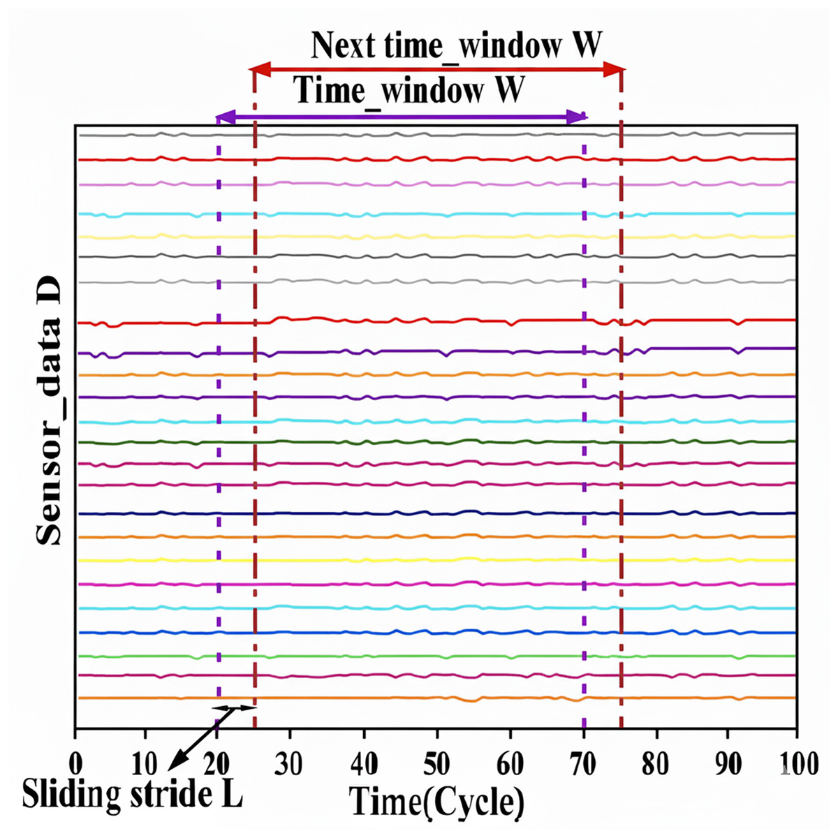
Figure 4: Sliding time window processing.
RUL labeling
Each entire sequence of takeoff, cruise, and landing is denoted as a cycle, and the aggregate count of cycles from the present flight cycle to the cycle of running until failure is designated as RUL. The RUL of an aero-engine is calculated by the following.
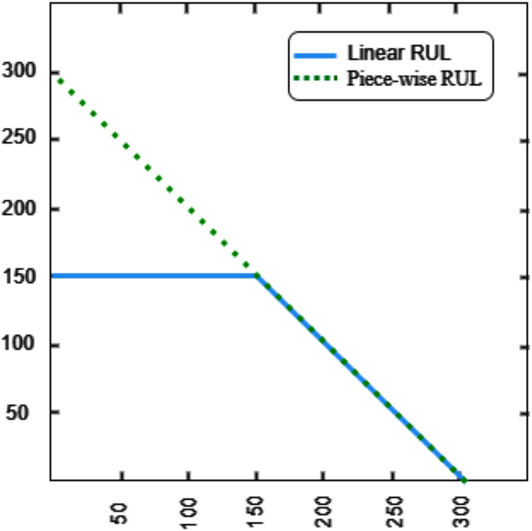
(12) where s indicates the aero-engine sample, indicates the maximum cycle number that can be performed, and indicates the current cycle number of the sample. A piecewise linear RUL is utilized as a substitute for the actual RUL. As shown in Fig. 5. The RUL of the aero-engine will be maintained at a consistent level until a fault arises. In this study, the maximum RUL value is more appropriate to set this constant value to 150. The following is how the RUL labels are configured.
(13) where t indicates time step.
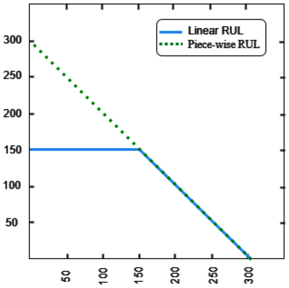
Figure 5: RUL labeling.
Prediction procedure
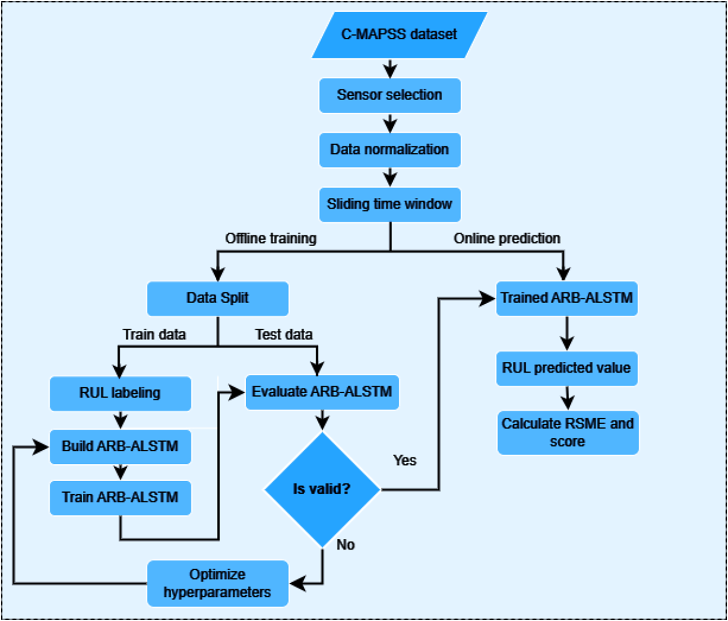
A flow chart for predicting the aero-engine’s remaining useful life using the DAB-LSTM model is illustrated in Fig. 6. For offline training of DAB-LSTM, the process begins by selecting suitable sensors from the C-MAPSS dataset for model training. Next, the sensor data is normalized using z-score normalization, followed by sliding time window processing. Training and testing datasets are then generated from the processed sensor data to serve as inputs for model training. After evaluation and hyperparameter optimization, a well-trained DAB-LSTM model is prepared for online predictions.
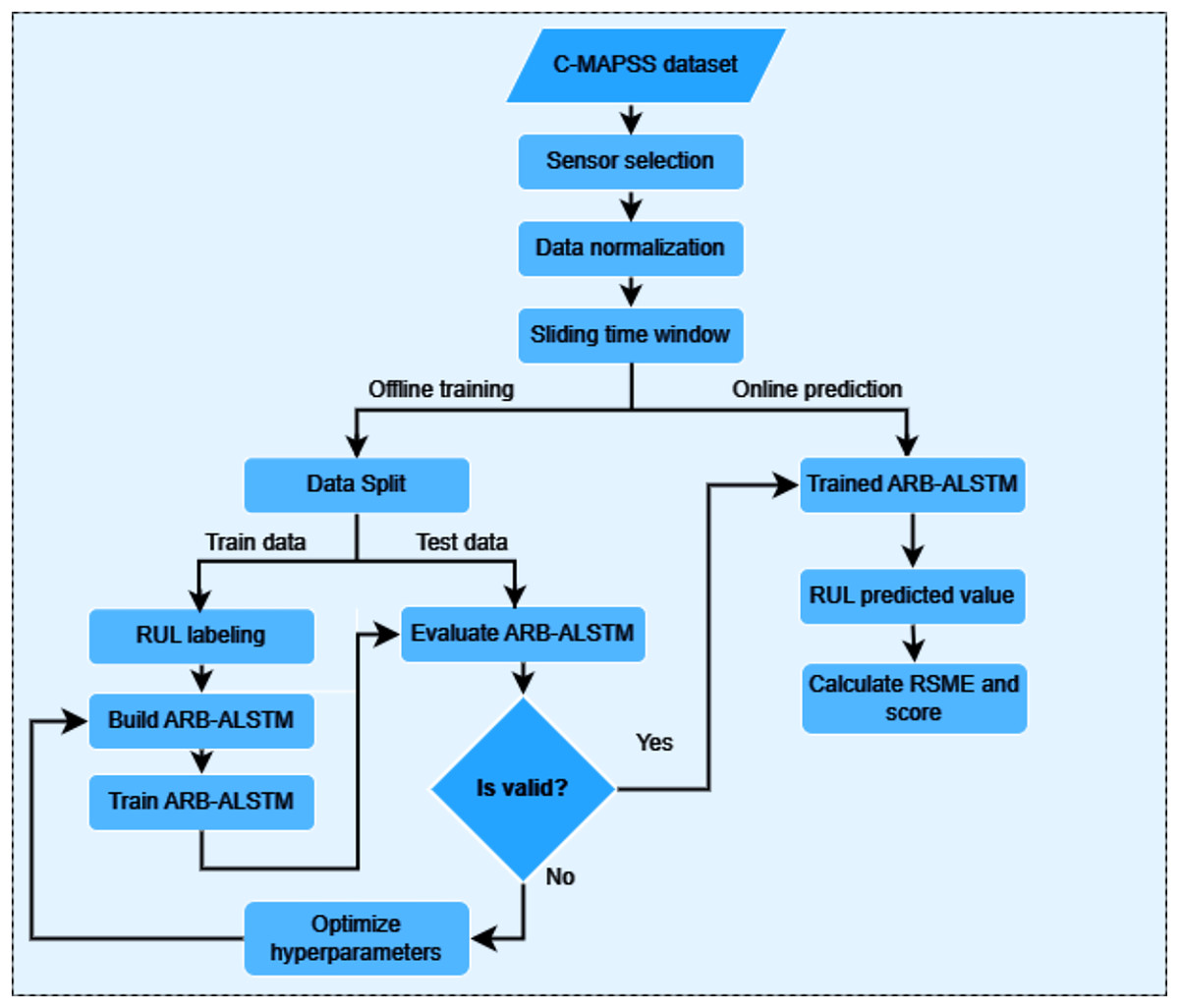
Figure 6: The AEB-ALSTM model flowchart.
Hyperparameter selection
The DAB-LSTM model under consideration incorporates various hyperparameters, including learning rate, batch size, dropout rate, and attention size, which must be precisely determined to enhance its efficacy. Consequently, this research employs the Optuna framework. Optuna serves as a hyperparameter optimization tool that utilizes sophisticated algorithms to effectively identify optimal hyperparameter configurations. Its principal search methodology is a sequential model-based optimization (SMBO) technique, specifically a variant of the TPE. Furthermore, Optuna accommodates additional algorithms, such as grid search and random search. The default primary algorithm utilized by Optuna is the TPE. Rather than directly modeling the objective function, TPE constructs two probability distributions: l(x) represents the probability of favorable parameter configurations (characterized by low loss values), while g(x) signifies the probability of all alternative configurations. The algorithm seeks to optimize the expected improvement (EI) in order to determine the subsequent set of hyperparameters to evaluate. It is particularly adept at optimizing both continuous and discrete hyperparameters. The hyperparameters of the DAB-LSTM model, such as window size, learning rate, batch size, dropout rate, and so on, are listed in Table 3. Moreover, a sensitivity analysis was conducted on key hyperparameters, including learning rate, dropout rate, and window size. The findings indicate that a dropout rate of 0.6 and a sliding window length of 31 yield optimal trade-offs between generalization and convergence stability, consistent with the hyperparameter configurations obtained via the Optuna-TPE optimization framework. The structural parameters of the proposed model on FD001 are listed in Table 4.
| Parameter | Value |
|---|---|
| Window size | 31/60 |
| Learning rate | 0.0002 |
| Batch size | 32 |
| Epoch | 120 |
| Attention size | 32 |
| Dropout rate | 0.6 |
| Optimizer | Adam |
| Loss | Score |
| Component | Layers | Parameters |
|---|---|---|
| Block_1 (path 1) | LSTM | units=256, activation=‘tanh’, regularizer=L1L2(l1=1e−5, l2=1e−3) |
| Block_2 (path 2) | Conv1D | Filters=32, kernel_size=2, padding=‘same’, activation=‘relu’, |
| Dropout | 0.6 | |
| Scaled dot-product | // scaled dot-product attention | |
| Dense | units=32, activation=‘relu’, | |
| LSTM | units=128, activation=‘tanh’, regularizer=L1L2(l1=1e−5, l2=1e−3) | |
| Adaptive attention | units=32 | |
| Repeat vector | // for repeat the output of adaptive to be tuple | |
| Block_3 | concatenate | // concatenate the out of path 1 and path 2 |
| LSTM | units=64, activation=‘tanh’, regularizer=L1L2(l1=1e−4, l2=1e−2) | |
| Dropout | 0.6 | |
| Block_4 | Dense (output) | units=1 |
Evaluation metrics
The root mean square error (RMSE) and score are used to evaluate the proposed model for predicting RUL performance. The Eq. (14) is used to calculate the RMSE value. RMSE serves as an indicator of the disparities between estimated values and actual values. The Eq. (15) is used to calculate the score value.
(14) where N indicates the total number of samples, i indicates the same number, indicates the true RUL of sample i, and indicates the predicted RUL of sample i. Contradicted to the RMSE metric, the scoring function gives higher weight to late predictions than early predictions, as defined in the following formula (Sateesh Babu, Zhao & Li, 2016):
(15) where . The method demonstrates superior performance when achieving lower values for RMSE and Score. In addition to RMSE and Score, the mean absolute error (MAE) metric was introduced to provide a more comprehensive evaluation of model performance. The Eq. (16) is used to calculate the MAE value. Unlike RMSE, which disproportionately penalizes large deviations, MAE measures the average magnitude of prediction errors, offering a balanced assessment of model accuracy and robustness to outliers. The inclusion of MAE aligns with best practices in recent PHM studies and strengthens the reliability of the comparative analysis.
(16)
Experimental results and analysis
Ablation study
To comprehensively assess the contribution of each architectural component, an extensive ablation study was performed to evaluate the individual and combined effects of the LSTM backbone, attention block, and adaptive attention mechanism within the proposed DAB-LSTM framework. Three model configurations were implemented for comparison: (i) a baseline LSTM-only network without any attention layers, (ii) an Attention-LSTM variant incorporating only the attention block, and (iii) the complete DAB-LSTM model integrating both the attention block and the adaptive attention mechanism. All models were trained under identical hyperparameter settings to ensure a fair evaluation. The results revealed that the LSTM-only baseline achieved stable performance but struggled to capture fine-grained temporal dependencies, resulting in higher RMSE and Score values. The addition of the attention block in the second variant led to a noticeable improvement, particularly in early fault detection, by allowing the model to focus on significant steps within the degradation sequence. However, as shown in Table 5, the integration of the adaptive attention mechanism in the full DAB-LSTM model yielded the most substantial gains, reducing RMSE by approximately 6.5–7% and MAE by 7–8% compared with the single-attention variant. This improvement confirms that the adaptive attention enables dynamic feature reweighting in response to be evolving degradation behavior, thereby enhancing robustness and generalization. The ablation findings clearly demonstrate that both attention modules contribute synergistically to model performance, validating the effectiveness and necessity of the proposed dual-phase attention design.
| Metrics | RMSE | MAE | Score |
|---|---|---|---|
| FD001 | 12.59 | 9.3 | 212.18 |
| FD003 | 12.38 | 9.2 | 221.52 |
RUL prediction
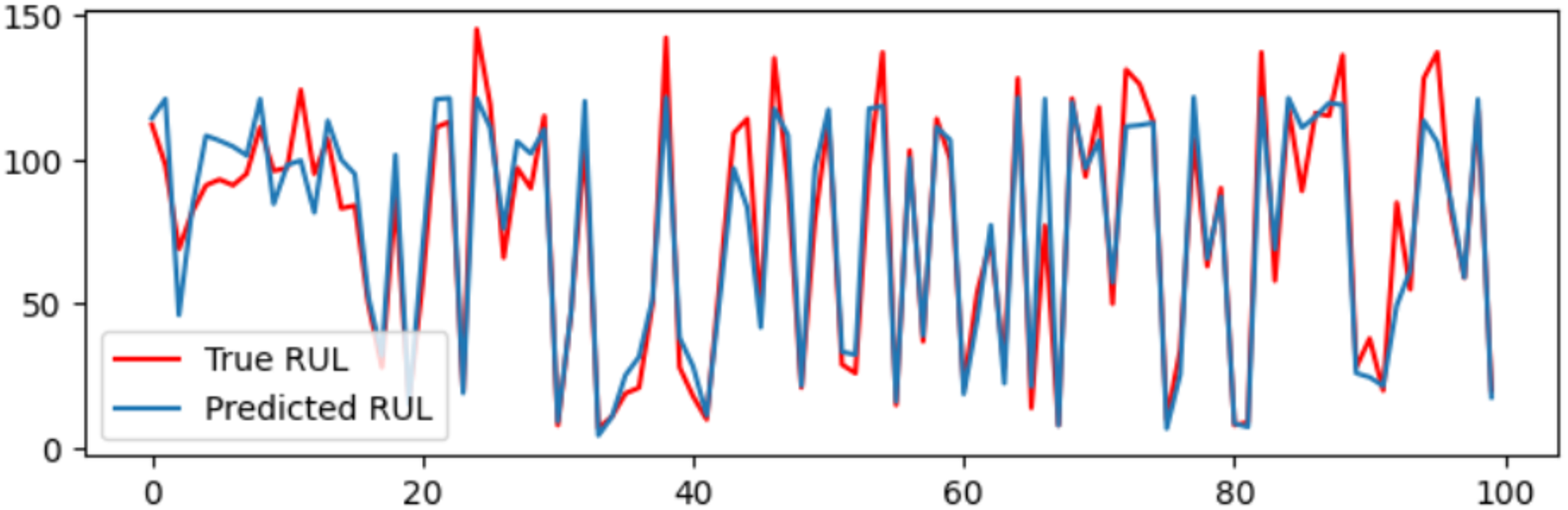
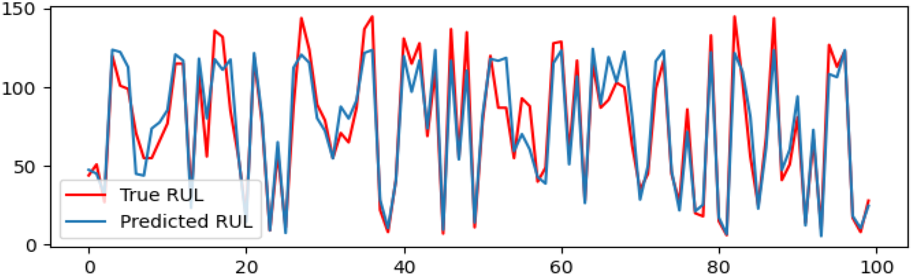
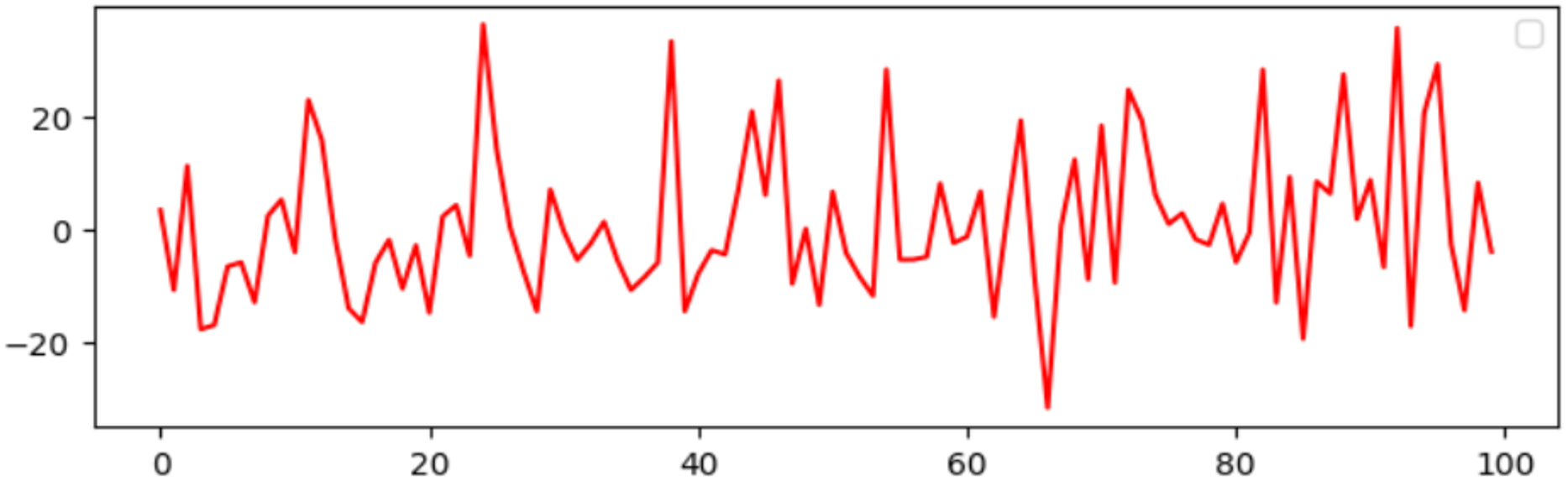
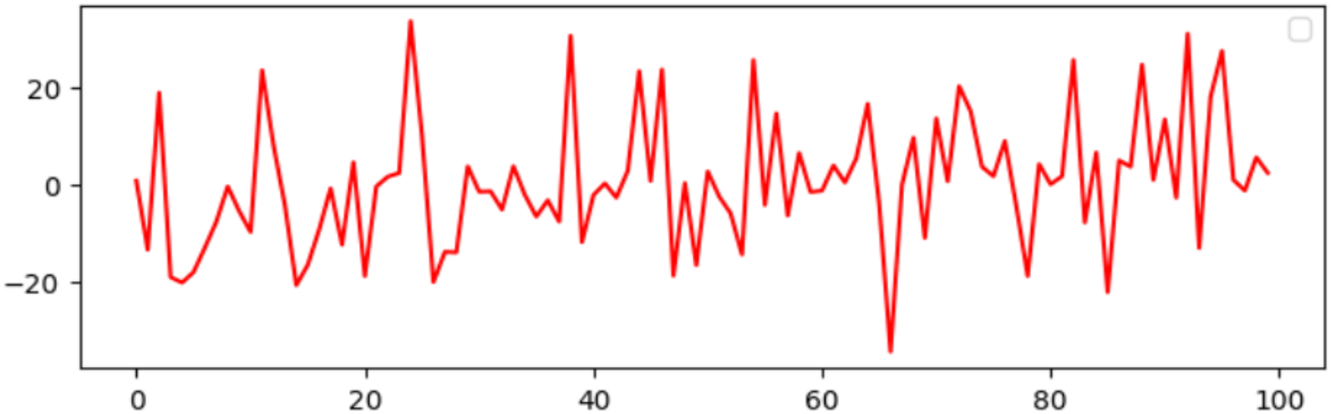
A DAB-LSTM model has been introduced to forecast the RUL of aero-engines. This section evaluates the actual RUL annotations against those predicted by the proposed DAB-LSTM for both FD001 and FD003 datasets to demonstrate the proximity of the predicted RUL to the true RUL. The predicted RUL values for each sample within the testing dataset are displayed alongside the corresponding actual RUL values. Figures 7 and 8 illustrate the discrepancies between the true and predicted values for the FD001 and FD003 datasets. It is evident from Figs. 7 and 8 that the RUL prediction values generated by the proposed model closely align with the actual RUL values for the FD001 dataset. To quantitatively assess the deviation between the predicted and actual RUL, Figs. 9 and 10 have been presented to depict the error for each test instance within the two analyzed sub-datasets. Additionally, Figs. 9 and 10 reveal that for both FD001 and FD003, the prediction errors are distributed within the interval [−30, 30]. Notably, the majority of the prediction errors are concentrated within the range of [−20, 20]. Most absolute errors remain below the size of a designated time window. The results of the model’s predictive performance on the test set are illustrated in Figs. 7, 8, 9, and 10. In Table 6, the RMSE values for the DAB-LSTM across the two sub-datasets are recorded as 12.59 and 12.38, while the MAE values are 9.3 and 9.2, respectively; the scores documented are 212.18 and 221.52, respectively. Based on the preceding analysis, it can be inferred that the proposed DAB-LSTM demonstrates considerable stability, as it achieves comparable performance across two distinct datasets, in addition to exhibiting robust efficacy in minimizing the divergence between the predicted and actual RUL.
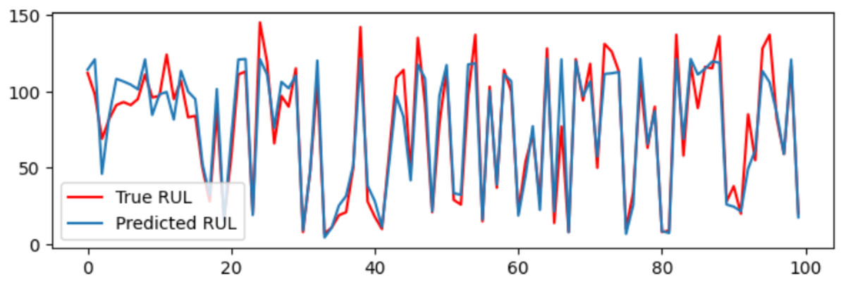
Figure 7: The true value and predicted value for FD001.
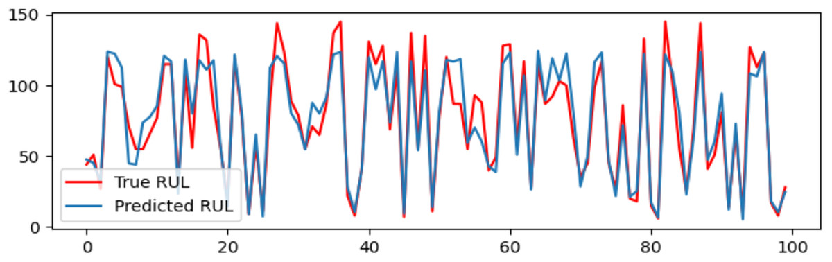
Figure 8: The true value and predicted value for FD003.
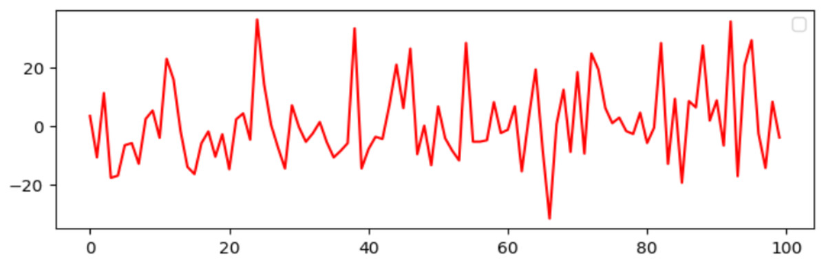
Figure 9: The prediction error for RUL on FD001.
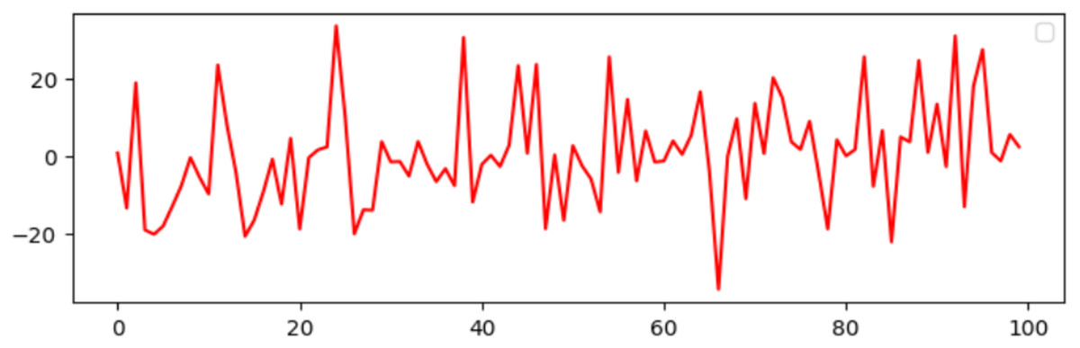
Figure 10: The prediction error for RUL on FD003.
| FD001 | FD003 | |||
|---|---|---|---|---|
| RMSE | Score | RMSE | Score | |
| BiGRU-AS (2021) | 13.86 | 284 | 15.53 | 428 |
| ELSTMNN (2021) | 18.22 | 571 | 23.34 | 839 |
| Bilstm attention (2021) | 13.78 | 255 | 14.36 | 438 |
| RVE (2022) | 13.42 | 323.82 | 12.51 | 256.36 |
| LSTM (2022) | 16.1 | 338 | 16.2 | 852 |
| DSAN (2022) | 13.4 | 242 | 15.12 | 497 |
| Att-LSTM (2022) | 13.95 | 320 | 12.72 | 223 |
| DCNN (2022) | 12.6 | 274 | 12.6 | 284 |
| KGHM (2023) | 13.18 | 251 | 13.54 | 333 |
| SAM-CNN-LSTM (2023) | 12.6 | 261 | 13.8 | 253 |
| Attention-LSTM (2023) | 15.45 | 455.92 | 14.67 | 473.97 |
| ABGRU (2023) | 12.83 | 221.54 | 13.23 | 279.18 |
| PINNs (2023) | 16.89 | 523 | 17.52 | 1194 |
| CP-LSTM (2024) | 13.59 | 224.88 | 12.94 | 207.1 |
| DA-LSTM (2024) | 12.62 | 263 | 13.34 | 360 |
| BayesLSTM (2024) | 13.26 | 265.76 | 12.68 | 242.91 |
| Proposed method | 12.59 | 217.18 | 12.38 | 221.52 |
A comprehensive interpretation of the results provides deeper insight into the mechanisms underlying the superior performance of the proposed DAB-LSTM framework. The model’s dual-phase attention architecture allows it to capture both long-term temporal dependencies and short-term degradation fluctuations, effectively integrating global and local information across the engine’s operational cycles. The attention block focuses on salient local features and critical sensor responses within each time window, while the adaptive attention mechanism dynamically adjusts attention weights according to the evolving degradation state, ensuring that the network prioritizes features most relevant to the current health condition. This adaptive behavior leads to more precise and stable RUL estimation across varying operational modes. Visualization of the learned attention weights further confirms that the model assigns higher importance to pressure, temperature, and rotational-speed sensors factors physically correlated with component wear and efficiency loss particularly during early and mid-stage degradation. This interpretable behavior not only strengthens the correspondence between the proposed model and underlying physical processes but also demonstrates that the improved predictive accuracy arises from meaningful, domain-aligned representations rather than overfitting or data artifacts. These findings underscore the scientific validity and practical value of the DAB-LSTM framework in real-world prognostics and health management applications.
Another strength of the DAB-LSTM is its inherent interpretability. By examining the learned attention weights, practitioners can identify which sensors and time steps were most influential in the model’s decisions. For instance, attention analysis revealed that sensor readings related to temperature and pressure fluctuations often received higher weights in early degradation stages. This insight can guide domain experts in understanding failure mechanisms and validating the model’s behavior, potentially facilitating trust and adoption in industrial settings.
The dual attention mechanism enhances both spatial and temporal feature extraction. By allowing the model to focus on critical time steps and sensor variables, it reduces the risk of overfitting to irrelevant patterns. This leads to improved generalization and stability across varying operational conditions. In comparison to other benchmark models such as vanilla LSTM and attention-LSTM, DAB-LSTM shows a marked improvement in predictive accuracy, particularly in early-stage fault progression where signal noise is higher.
Comparisons with other algorithms
Moreover, we systematically assess the efficacy of the suggested DAB-LSTM framework for RUL prediction. To establish its merit, we juxtapose the proposed model with a range of established methodologies that are broadly acknowledged within the discipline. These methods include BiGRU-AS (Duan et al., 2021), ELSTMNN (Cheng et al., 2020), BiLSTM attention (Liu et al., 2021), RVE (Costa & Sánchez, 2022), LSTM (Chen et al., 2022), DSAN (Xia et al., 2022), Att-LSTM (Boujamza & Elhaq, 2022), DCNN (Zhang et al., 2022), KGHM (Li et al., 2023), SAM-CNN-LSTM (Li et al., 2023), Attention-LSTM (Cheng et al., 2023), ABGRU (Lin et al., 2023), PINNs (Liao et al., 2023), CP-LSTM (Arunan et al., 2024), DA-LSTM (Liao et al., 2023), and BayesLSTM (Xiang et al., 2024). Table 7 shows the comparison results. The results of DAB-LSTM for both FD001 and FD003 are juxtaposed against those of 16 competing models to demonstrate its efficacy and efficiency. These results are conveyed in terms of RMSE and Score metrics.
| Metrics | RMSE | MAE | Score |
|---|---|---|---|
| FD001 | 12.59 | 9.3 | 212.18 |
| FD003 | 12.38 | 9.2 | 221.52 |
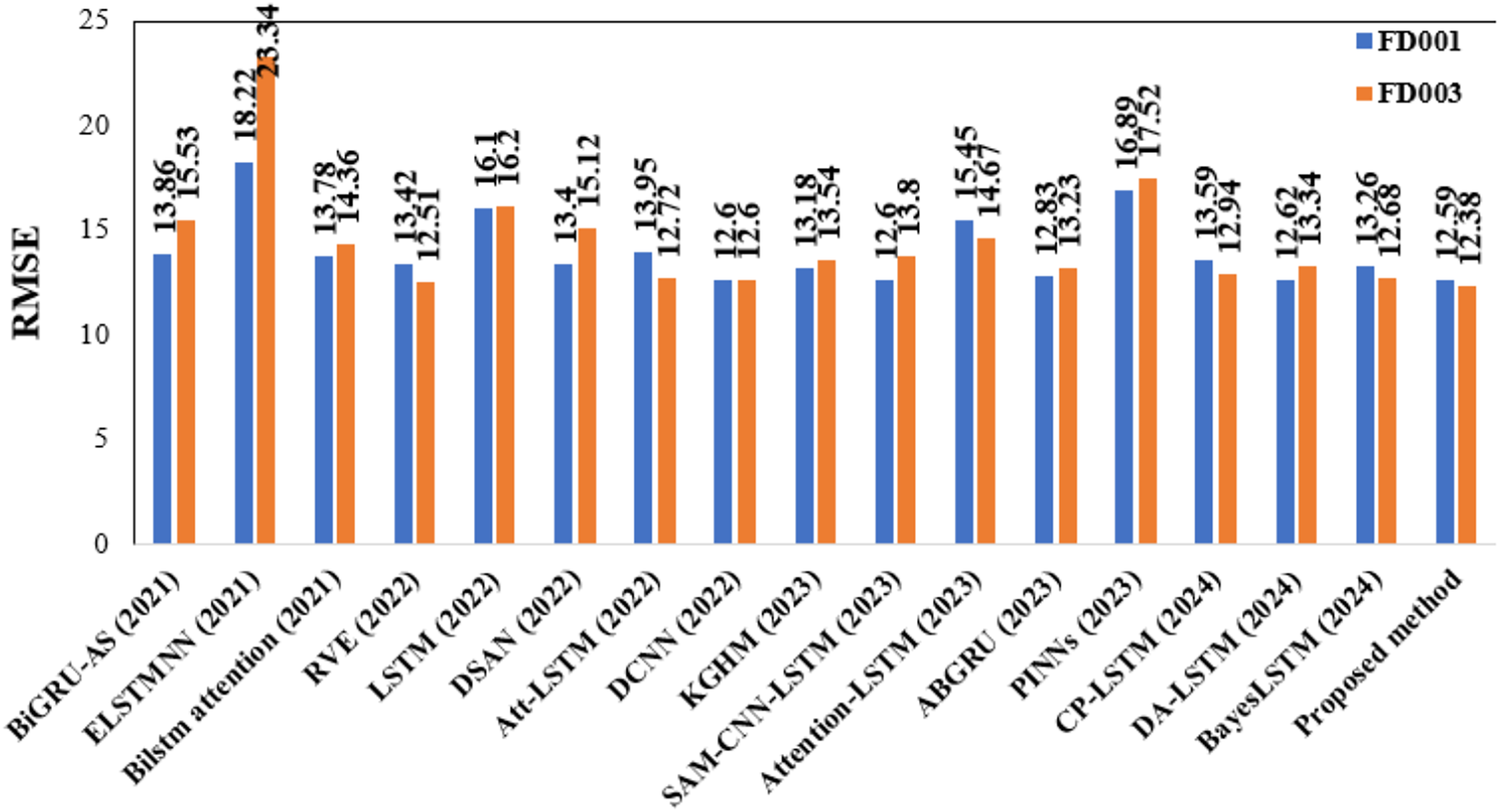
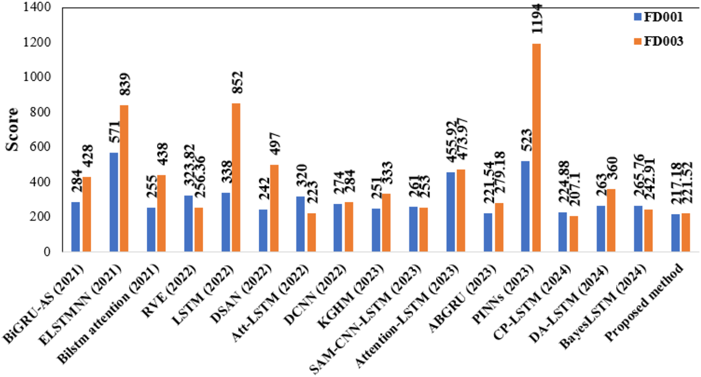
As delineated in Table 7, the proposed DAB-LSTM architecture consistently exceeds the performance of current RUL prediction models across the FD001 and FD003 datasets, thereby illustrating its enhanced predictive efficacy. Specifically, for the FD001 dataset, our approach exhibits optimal performance, achieving the minimal RMSE and Score values. The proposed model is considered the best because it achieves the lowest RMSE, a metric that gives equal weight to both late and early predictions. On the contrary, the scoring metric assigns greater weight to late predictions than to early ones, thereby favoring models that better handle late-stage degradation. Notably, the DAB-LSTM framework demonstrates substantial advancements in both the RMSE and Score metrics for the demanding FD001 dataset, surpassing the leading models in both aspects. For the FD003 dataset, our DAB-LSTM architecture secures the highest performance regarding both RMSE and Score metrics. Figures 11 and 12 are presented to show the RMSE and Score values obtained by various algorithms for the two considered sub-datasets.
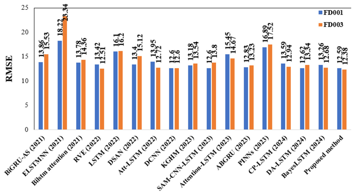
Figure 11: Depiction of RMSE values obtained by various models.
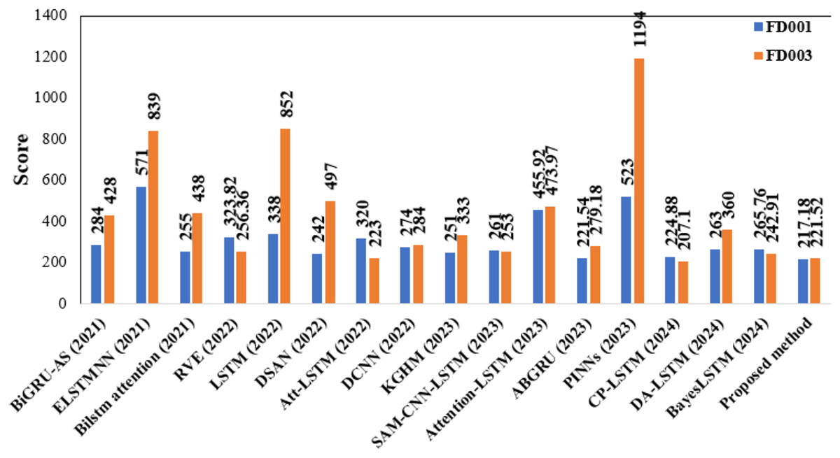
Figure 12: Depiction of score values obtained by various models.
This study is constrained by several limitations. First, the exclusive use of the NASA C-MAPSS FD001 dataset restricts the generalizability of the findings, as it does not encompass the full spectrum of engine degradation patterns or varying operational scenarios. Second, the computational environment limited to two CPU cores and 12 GB of RAM constrained the investigation of more advanced model architectures and hindered comprehensive scalability assessments. Furthermore, while attention mechanisms highlight feature importance, the model lacks explicit explainability frameworks (e.g., SHAP, LIME) to justify predictions to domain experts.
While DAB-LSTM performs well on the FD001 and FD003 datasets, it has not yet been extensively validated on other operating conditions represented in FD002 and FD004. Future work will involve assessing generalizability across multi-operating and multi-fault conditions. Additionally, integrating domain knowledge through physics-informed neural networks or hybrid models may further improve prediction accuracy and reliability. Lastly, exploring transformer-based architectures with similar dual-attention patterns may offer new perspectives on long-sequence modeling for RUL tasks.
Conclusions
This study presented a novel deep learning framework called DAB-LSTM, designed to enhance RUL prediction for aero-engines. By integrating both temporal and feature attention mechanisms, the proposed model effectively captures critical time-dependent patterns and sensor-level features that are often overlooked by traditional LSTM and CNN-LSTM architectures. Experimental validation using the FD001 and FD003 subsets of the C-MAPSS dataset demonstrated that DAB-LSTM significantly outperforms existing methods. These improvements highlight the model’s robustness and precision in handling complex degradation trajectories.
Beyond performance gains, the dual attention mechanism contributes to the interpretability of the model, enabling insights into which time steps and sensor signals most influence the RUL predictions. The DAB-LSTM also exhibits strong generalization and computational efficiency, making it suitable for real-world deployment in predictive maintenance systems.
Future work will extend this model to handle diverse operating conditions and fault types present in other C-MAPSS subsets and explore integration with physics-based insights and transformer-based architectures. Overall, the DAB-LSTM offers a compelling and scalable solution for data-driven prognostics in complex industrial systems.