
Benchmarking augmentation to enhance A-line and B-line classification with sparse data
- Published
- Accepted
- Received
- Academic Editor
- Consolato Sergi
- Subject Areas
- Artificial Intelligence, Computer Vision, Data Mining and Machine Learning, Optimization Theory and Computation, Neural Networks
- Keywords
- A-lines, Augmentation methods, B-lines, Image classification, Lung artifacts, Lung ultrasound, Medical image processing, Ultrasound
- Copyright
- © 2026 Hliboký et al.
- Licence
- This is an open access article distributed under the terms of the Creative Commons Attribution License, which permits using, remixing, and building upon the work non-commercially, as long as it is properly attributed. For attribution, the original author(s), title, publication source (PeerJ Computer Science) and either DOI or URL of the article must be cited.
- Cite this article
- 2026. Benchmarking augmentation to enhance A-line and B-line classification with sparse data. PeerJ Computer Science 12:e3436 https://doi.org/10.7717/peerj-cs.3436
Abstract
In real-life medical applications, there is often no curated data available for training machine learning solutions. In this article, we explore the efficacy of various ways of addressing this issue, such as extending the training set using historical data, data transformation, and data augmentation. We conducted experiments on lung ultrasound data for A-line and B-line artifact detection. The dataset used was acquired from real-life examinations done in a hospital where physicians labeled approximately every tenth frame, resulting in sparsely labeled data. We expanded this dataset using historical ultrasound scans from various probe types and evaluated two transformation strategies—standard resizing and edge padding—alongside several augmentation methods. The biggest improvement in F1-score was from 0.69 to 0.86 for A-line detection, and from 0.53 to 0.8 for B-line detection. These results prove the utility of carefully chosen data transformation and augmentation when training on sparsely labeled data.
Introduction
Lung ultrasound (LUS) has emerged as an effective diagnostic tool, particularly during the COVID-19 pandemic (Demi et al., 2023; Yang et al., 2023; Boccatonda & Piscaglia, 2024). It can swiftly and accurately detect lung problems, which is helpful in intensive care and emergency settings. LUS is capable of detecting a variety of conditions affecting the outer areas of the lungs, such as collapsed lungs (pneumothorax) (Fei, Lin & Yuan, 2021), fluid buildup caused by heart failure or infections (pulmonary edema) (Dong et al., 2023), lung infections (pneumonia) (Boccatonda et al., 2023), severe lung injury (acute respiratory distress syndrome) (Boumans et al., 2024), fluid between the lung and chest wall (pleural effusion) (Hansell et al., 2021), and blockages in the lung’s blood supply (pulmonary infarction), among others (Demi et al., 2023).
LUS differs from conventional imaging methods: instead of providing direct anatomical images, it seeks out sonographic artifacts. This is necessary because the air in the lungs hinders ultrasound waves from fully penetrating the lung tissue. LUS primarily identifies specific artifact patterns, such as A-lines and B-lines, which signify various lung conditions (Soldati et al., 2019; Volpicelli et al., 2012).
A-lines are horizontal, hyperechoic lines that indicate normal lung aeration, while B-lines are vertical, comet-tail-like artifacts associated with abnormalities such as pulmonary edema, interstitial lung disease, and other pulmonary conditions. Detecting these artifacts is essential in LUS interpretation, as A-lines typically represent healthy, well-aerated lung regions, whereas the presence, number, and distribution of B-lines are strong indicators of pulmonary pathology. Recognizing these patterns enables timely and accurate diagnosis, guiding appropriate treatment decisions and potentially reducing morbidity and mortality in patients with acute respiratory failure.
Despite their clinical significance, identifying A-lines and B-lines remains challenging. Detection often relies on clinician expertise and subjective interpretation (Muñoz et al., 2024). The artifacts can appear subtle or blurred, and are sometimes difficult to distinguish from other ultrasound artifacts such as Z-lines and E-lines. Image quality is further influenced by equipment variability, operator skill, and patient-related factors such as positioning and movement, all of which can impact diagnostic consistency. Indeed, studies report poor to moderate reproducibility across different raters and ultrasound systems (Haaksma et al., 2020). To address these limitations, recent advances in artificial intelligence—particularly deep learning—are enhancing the accuracy and consistency of A-line and B-line detection, offering the potential to support more reliable and automated diagnostic workflows (Abbasi et al., 2025).
In practical terms, LUS offers an advantage over chest X-ray (CXR) and computed tomography (CT) imaging for quick bedside evaluations. Its non-invasive nature, absence of ionizing radiation, and ability to provide instant results make it particularly applicable in settings with limited imaging resources or where rapid decision-making is needed (Jakobson et al., 2022; Elabdein et al., 2024; Malík et al., 2023). Moreover, recent advances in artificial intelligence (AI) have boosted LUS’s effectiveness. AI helps to automate pattern recognition, enhances diagnostic precision, and minimizes operator discrepancies. Nhat et al. (2023) showed that integrating AI into lung ultrasound interpretation improved accuracy in detecting lung pathologies such as A-lines and confluent B-lines. Clinicians using the AI tool were more efficient in diagnosing and monitoring lung conditions, resulting in faster diagnosis and increased confidence levels. The AI tool was found to be helpful for both real-time and post-exam evaluation of lung ultrasound imaging. However, this and similar research projects still required carefully annotated and curated datasets that limit their applicability due to data sensitivity and different examination procedures in different medical institutes.
Yang et al. (2023) and Wang et al. (2022) provided detailed insights into the use of machine learning techniques in LUS up to 2022. Building upon these studies, we now highlight more recent contributions. Lucassen et al. (2023) introduced a novel LUS dataset with expert annotations, containing 1,419 videos from 113 patients labeled for B-line presence. Utilizing this dataset, they benchmarked deep learning (DL) methods for B-line detection across multi-frame clips, single frames, and individual pixels (segmentation). Their innovative approach to B-line localization works on the level of pixels, representing origin locations as single points. The research was limited by the use of a dataset collected in a single hospital while validation across diverse clinical settings is needed.
Xing et al. (2023) proposed a new technique for detecting A-lines in LUS images. They combined an enhanced Faster R-CNN model with a selection strategy of localization boxes to identify the pleural line accurately. This allowed them to segment the LUS images below the pleural line for independent analysis not influenced by similar structures. The authors then used a method utilizing total variation, a matching filter, and grayscale differences for automatic A-line detection. The experiment involved training the model on 3,000 convex array LUS images and testing it on 850 convex array and 1,080 linear array LUS images. The reported accuracy of the A-line detection system was 93.39% and 91.90% for convex and linear probes, respectively. Building on their previous work, Xing et al. (2024) employed a novel cascaded deep learning model based on convolution and multilayer perceptron to locate and segment the pleural line in lung ultrasound images. Using gray-level co-occurrence matrix and self-designed statistical methods, they extracted eight textural and three morphological features to characterize the pleural lines. Machine learning-based classifiers were then used to evaluate the lesion degree of pleural lines in lung ultrasound images. A prospective evaluation was conducted on 5,390 images from 31 pneumonia patients, achieving a Dice score of 0.87 and an accuracy of 94.47%.
Howell et al. (2024) introduced a real-time multi-class segmentation technique for accurately detecting specific anatomical features and artifacts in lung ultrasound images. They used a lightweight U-Net model trained on a dataset of lung ultrasound phantom images and successfully identified and segmented ribs, pleural lines, A-lines, B-lines, and B-line confluence with notable accuracy. The mean Dice Similarity Coefficient (DSC) exceeded 0.7, indicating high accuracy in artifact detection even with a minimal training dataset of only 300 images.
The study conducted by Li et al. (2023) does not directly identify lung artifacts, but it is able to detect and classify medical video sequences with minimal frame-level supervision. The researchers used a weakly semi-supervised approach, combining frame detection with video classification. They created “tracklets” by aggregating individual predictions from a detection model, which represented consistent regions of pathology over time. These tracklets were then classified to provide an overall prediction for the entire video.
Previous research often relied on datasets curated specifically for the purposes of artifact detection. In real-life scenarios, however, only a limited amount of training data is available due to a lack of standard datasets that could be applied for various LUS imaging applications. Labeling further data is time-intensive and often infeasible due to the limited time medical experts can spend on data acquisition and labeling. Our study examines whether incorporating historical data acquired from different ultrasound probes into a limited LUS dataset can improve the performance of models in classifying sonographic artifacts. Specifically, we focus on detecting the presence of clinically relevant LUS artifacts, A-lines and B-lines, through classification rather than segmentation. We also evaluate the effect of various preprocessing and data augmentation techniques to improve model generalization. This dual focus on dataset enhancement and artifact classification aims to support the development of robust AI tools in settings where labeled medical imaging data is scarce. Our results offer insights into how selection of preprocessing and augmentation methods can improve performance in LUS artifact detection tasks.
The key contributions of our study are:
-
1.
Empirical comparison of different image preprocessing methods and their impact on model performance;
-
2.
Proposing data processing and training methodology for A- and B-line detection;
-
3.
Exploring the possibility of using historical data for improved model performance.
Methodology
The aim of this study is to develop AI-based classification models that can detect the presence of clinically relevant sonographic artifacts—A-lines and B-lines—in LUS frames. The primary focus is on evaluating how training dataset characteristics (probe diversity, preprocessing methods, and augmentation techniques) influence classification performance. Importantly, this study is not focused on segmentation or localization tasks. Instead, we treat artifact detection as a binary classification problem at the frame level.
Data acquisition was performed at the Department of Thoracic Surgery and the Clinic of Radiology at Jessenius Faculty of Medicine in Martin, Slovakia, where LUS examinations were conducted following the standardized Bedside Lung Ultrasound in Emergency (BLUE) protocol, as described in Števík et al. (2024). Briefly, three experienced clinicians—one radiologist and two thoracic surgeons—performed the LUS assessments. Each patient underwent a single session in the supine position. Ultrasound probes were placed at three BLUE points on each side of the thorax: the upper BLUE point, lower BLUE point, and the Posterolateral Alveolar and/or Pleural Syndrome (PLAPS) point, following the recommendations by Lichtenstein & Mezière (2011). Videos were recorded at each point during normal breathing, yielding six videos per patient.
Prior to inclusion in the study, each participant received both oral and written information about the study procedures, objectives, and data handling. Participation was voluntary, and patients who agreed to take part signed a written informed consent form. Patient identity was anonymized by replacing names with study numbers and removing all identifying metadata from the recordings. Ethical approval for processing and analysis of the ultrasonographic video recordings was granted by the Ethics Committee of Jessenius Faculty of Medicine, Comenius University in Martin (Protocol No. EK 44/2021).
We planned to train the models on data from Philips Lumify probe. Due to the limited amount of data collected with this probe, we extended the dataset with imagery previously acquired using Sonoscape and Hitachi probes. All data was collected at the same hospital during routine patient examinations. This approach differs from the majority of present works as the data we use was not specifically curated for the purposes of model training but gathered in a real-world scenario.
The unfiltered dataset contains data including videos captured using radial probe tracks. Based on medical experts’ requirements, only data obtained via linear probes were used in training our models. While linear probes offer limited depth penetration compared to radial or convex transducers, this was considered acceptable given the study’s focus on detecting near-field artifacts. This selection criterion ensured more consistency and homogeneity. However, it is important to note that since recordings from real patient examinations were used, there is still some degree of variability, e.g., in depth and other probe settings. Only the frequency was fixed to 30 frames per second to minimize the effect of artifacts moving between labeled frames. The acquisition parameters were set based on the radiologist’s discretion and were not recorded for further reference as this would be unlikely to be done in future application.
Lung artifacts
During LUS examination, the examiner searches for artifacts, evaluates them, and derives the lung condition. These artifacts result from the varying effect of the tissues on ultrasound waves, i.e., reflection, scattering, refraction, and attenuation. Not all artifacts suggest the presence of disease; the presence of some, however, precludes the occurrence of others due to the essence of their physical properties. Several organs, such as the liver and spleen, are also important to locate when evaluating pathologies such as pleural effusion.
LUS examination starts by placing the probe in the intercostal space between two ribs, and by searching for the pleural line. The pleura cushions the lungs and chest cavity. The pleural line consists of two distinct layers: the parietal pleura is a membrane that covers the surface of the pleural cavity, the visceral pleura is a thin, slippery membrane that covers the surface of the lungs. A small amount of fluid in the pleural cavity eliminates friction and allows sliding of the parietal and the visceral pleura during breathing. This causes the lung ultrasound artifact called lung sliding, a sliding motion of the pleural line in lung ultrasound recordings. The pleura is visible in every ultrasound image (if the depth of the ultrasonography (USG) probe is correctly set) and serves as a basic navigation point. It is the first horizontal line/artifact in the analysis of LUS video by doctors (Finley & Rusch, 2011).
After identifying the pleural line and the evaluation of the presence and abscence of lung sliding, two other LUS artifacts are searched for, A- and B-lines. Mostly, their presence or absence alone does not indicate a specific pathology. It is important to evaluate the combined occurrence, distribution and prevalence of these artifacts.
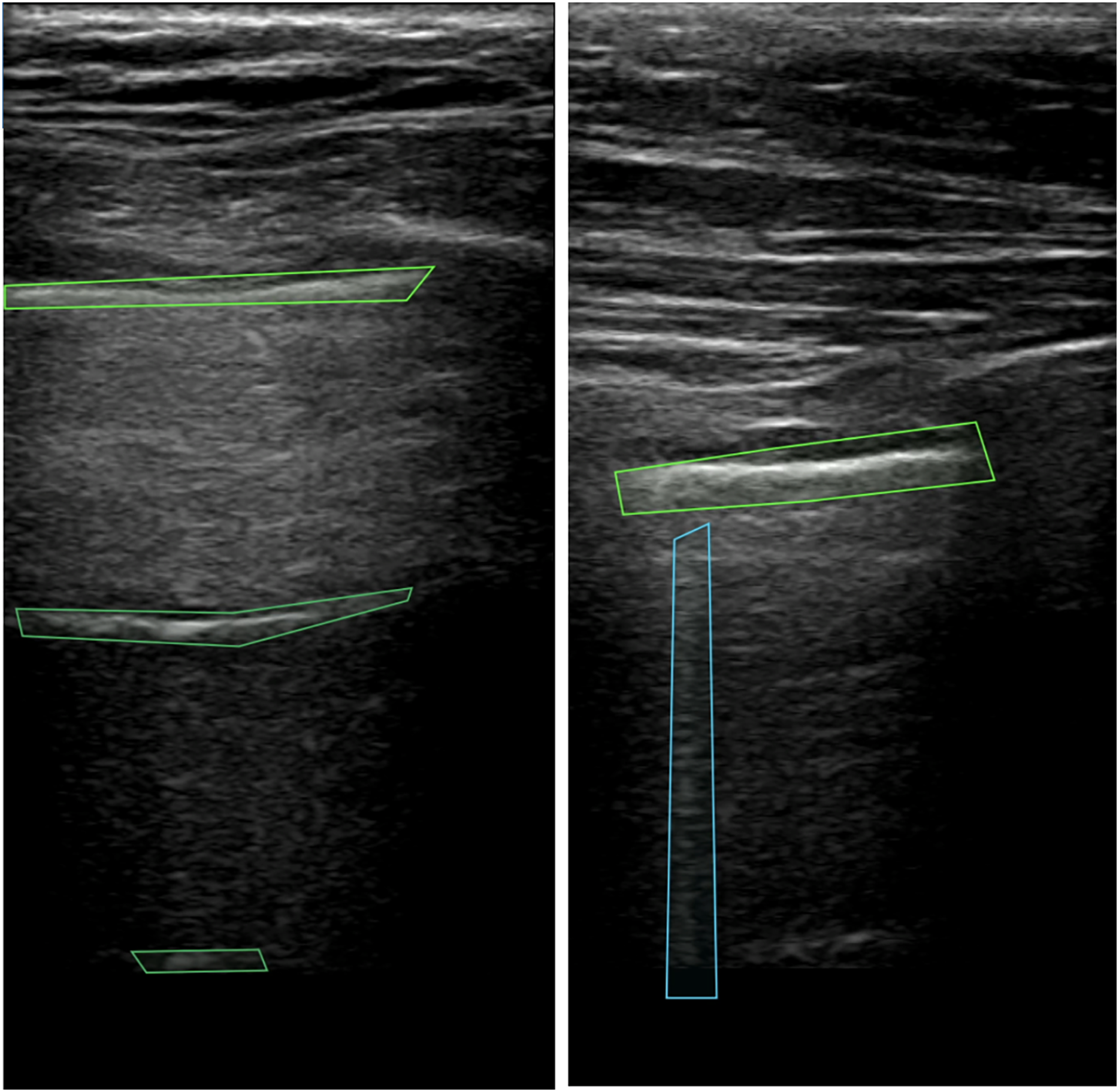
A-lines represent repeated reflections of the pleura manifested as bright horizontal lines. The pleura (see top green box in Fig. 1) is always visible as the first line closest to the probe. The remaining horizontal lines appear below the pleural line at the same distance from each other as the distance between the probe and the parietal line. Artifacts that resemble A-lines but deviate from the equidistant pattern are considered suspicious and require further investigation. For the detection of A-lines, the depth of visible area should be set properly on the machine, otherwise, for example if excessive subcutaneous fat is present, it may be impossible to evaluate the presence of this artifact (Lichtenstein, 2014). In the case of lung sliding absence, observation of A-lines supports but does not definitely confirm the presence of pneumothorax (Volpicelli et al., 2012). This combination of artifacts may be also seen by patients with lung emphysema without pneumothorax.
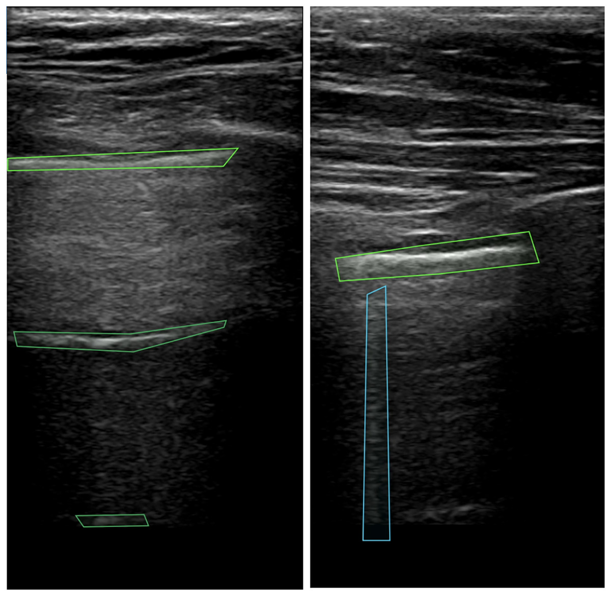
Figure 1: Pleura and A-lines (green polygons) and B-lines (blue polygon) in LUS images (Hliboký et al., 2023).
B-lines (see blue box in Fig. 1) are vertical artifacts arising from the pleural line extending indefinitely and erasing A-lines. Caused by fluid or cells in the sub-pleural region, the lung tissue creates discrete microscopic 3-dimensional aerated structures surrounded by fluid or cells. Under these circumstances, air/liquid interfaces act as specular reflectors, discrete reverberation foci, thus creating vertical beam-like artifacts (Wang et al., 2017). When evaluating B-lines, it is important to take the number and distribution of this artifact into account. Finding 2 or 3 B-lines in one intercostal space may be physiological. More B-lines call for a broader differential diagnosis, B-line presence excludes pneumothorax (Lichtenstein, 2014, Volpicelli et al., 2012).
Data labeling
For labeling, doctors used a colaborative software, the Computer Vision Annotation Tool (CVAT) (CVAT.ai, 2023). This tool offers a set of features tailored for medical image annotation, allowing for efficient and accurate labeling of anatomical structures and pathological features. The use of CVAT streamlines the annotation workflow, promoting consistency and reliability in labeled datasets in various domains. It also allows USG videos to be exported together with labeling and all metadata in standardized formats for easy data processing.
In the annotation process, doctors delineated the boundaries of the detected artifacts by multi-polygonal markers and indicated their class. Every video in our dataset was recorded at 30 frames per second (FPS). Due to time constraints, doctors labeled only every 10th frame of the video. Each video was labeled by one doctor and the annotations were then reviewed by another expert. In case of discrepancies, the two experts reached an agreement through discussion; in some cases the opinion of a third expert was also considered. The labeling process was followed by data cleaning supervised by an IT specialist.
The experiments described here were focused on classification only. Therefore, we do not work with the labeling polygons. Only the information about the presence or absence of a given sign on the frame is considered.
Data processing and filtering
LUS videos recorded by USG machines contained metadata such as probe settings, gain, measurement points, etc. These metadata did not overlap with the USG image area and were therefore removed from video frames. We implemented a simple preprocessing script that detected the USG area in the videos by discerning it from the black background. Our solution is applicable with USG devices of various brands and with various probe types. The information regarding the type of USG device used for data acquisition was retained to maintain comprehensive metadata integrity.
Next, we conducted video filtering and categorization. If a single frame of a video contained multiple distinct types of signs, the video was removed to reduce ambiguity in the dataset and minimize potential issues during model training. If A-lines or B-lines were present in one or more frames, the entire video was labeled as positive for that artifact; otherwise, it was labeled as negative. Table 1 provides a quantitative breakdown of the number of labeled videos per artifact class and ultrasound probe type.
| Probe class | ||||
|---|---|---|---|---|
| Video type | All | Lumify | Hitachi | Sonoscape |
| No lines | 59 | 15 | 29 | 15 |
| A lines | 39 | 18 | 15 | 6 |
| B lines | 33 | 17 | 13 | 3 |
The dataset analysis revealed notable differences in the occurrence of pathological signs, particularly between A-lines and B-lines, across the labeled frames within each video. On average, a video encompasses approximately 37 labeled frames, with each frame annotated for the presence or absence of specific pathological features.
In our dataset, A-lines occur at a notably higher rate, being present in 67% of the labeled frames. B-lines were identified in 29% of the labeled frames (see Tables 2 and 3, respectively).
| Video type | All | Lumify | Hitachi | Sonoscape |
|---|---|---|---|---|
| All labeled frame | 1,540 | 649 | 524 | 367 |
| Frame with A-lines | 1,075 | 448 | 395 | 232 |
| Usable frame [%] | 69.81 | 69.03 | 75.38 | 63.22 |
| Video type | All | Lumify | Hitachi | Sonoscape |
|---|---|---|---|---|
| All labeled frame | 1,204 | 441 | 601 | 162 |
| Frame with A-lines | 348 | 165 | 154 | 29 |
| Usable frame [%] | 28.90 | 37.41 | 25.62 | 17.90 |
Multiple LUS recordings were acquired from every patient in this research. In the medical domain it is important to ensure patient split while training models–videos from one subject should be used for a single purpose only–for training, validation or testing of the model. If images from the same patient (or ultrasound video) appear in both training and test sets, a model may learn patient-specific patterns instead of generalizable features, inflating performance metrics. During LUS examination, doctors record videos from six different locations on the chest. By capturing various regions of the thorax, the morphological overlap of the videos from the same patient is minimized. In this case, splitting videos from a single patient but from different locations is admissible between different subsets.
To address class imbalance and ensure proper evaluation of our experiments, we employed stratified 5-fold cross-validation. The dataset was split into training and test sets such that each fold maintained a uniform distribution of probe types and video classes, allowing for balanced representation across all subsets.
We created binary classification models for the classification of each sign separately (A-lines, B-lines). Negative examples were selected from videos labeled as showing no lines. Valid labeled frames were selected for each video, ensuring a balanced representation across classes. In cases where the positive class contained fewer frames than the negative class across all videos, we applied uniform frame dropping from each “No Lines” video to balance class distribution.
We applied negation sampling: in the A-line classification model, the negative class contained “No Lines” and also B-lines examples, and vice versa. The opposite class was balanced using the same frame-dropping technique employed for the negative class in the previous step.
Models
In our study, we used ResNet backbones. ResNet is a well-established convolutional neural network (CNN) architecture proposed in He et al. (2016). ResNet stands out for its innovative use of residual blocks, composed of two convolutional layers with Rectified Linear Unit (ReLU) activation functions. The main distinction of the ResNet block is the inclusion of a non-parameterized shortcut connection. This shortcut connection efficiently passes the output of the previous block directly to the next block without any modification. This design mitigates the vanishing gradient problem and facilitates the training of deeper networks.
During our experiments, we explored different variants of ResNet architectures, including ResNet-18, ResNet-34, and ResNet-52. The primary difference between these architectures is the number of residual blocks employed. Larger architectures can be used for more complex problems but they also have a higher tendency to overfit. During our primary experiments, overfitting occurred with larger models. To mitigate this risk, we conducted comparative experiments and focused on ResNet-18 because of its lower complexity and higher generalization performance.
Besides ResNet, we included Inception architecture (Szegedy et al., 2015) for evaluation alongside ResNet to broaden our comparative analysis. Inception modules serve as a fundamental framework for addressing scale variation within images, thereby enhancing the network’s ability to capture multi-scale features effectively (McNeely-White, Beveridge & Draper, 2020).
The distinguishing feature of Inception modules is their use of convolutional layers at different sizes in conjunction with max pooling using the same input. Subsequently, the outputs from these operations are concatenated together, enabling the model to extract diverse feature maps while maintaining a relatively shallow depth compared to other architectures. We selected the Inception-v3 architecture for our experiments due to its frequent use in medical image analysis.
The training process adhered to established practices to ensure efficacy of the models. We trained separate models for each task via transfer learning, using models pre-trained on the ImageNet dataset to ensure fast convergence. For each model type, we carried out empirical testing with a base model, on which all training hyperparameters were optimized. Later on, the same values were used in all experiments. The learning rate was set to 0.001, and the input resolution to pixels, balancing computational efficiency and image detail. Employing the Adam optimizer and early stopping with a patience of 5 epochs mitigated the risk of overfitting. The Binary Cross-Entropy loss function was chosen for its suitability in binary classification tasks.
All training was done on Nvidia RTX A500 24GiB vRAM cards with CUDA version 12.2.1.020. The source code was implemented and run in Python 3.9 with Pytorch 2.13 and MONAI 1.2. For optimal performance, we used the NGC Pytorch container environment (version 23). Experiment results were logged in wandb.
Preprocessing methods
Images sourced from various origins needed to be rescaled to fixed input dimensions compatible with the chosen CNN. This is commonly done using interpolation (Chansong & Supratid, 2021). All down/upsampling was performed with bicubic interpolation. Bicubic kernels preserve local gradient structure better than bilinear and avoid the aliasing artefacts that nearest-neighbour causes in high-frequency speckle regions (Hashemi, 2019; Hirahara et al., 2021). Ultrasound videos are typically taller than they are wide, a result of the ultrasound probe’s scanning angle or the imaging device’s acquisition characteristics, as illustrated in Fig. 2. Consequently, resizing these images by stretching them horizontally may distort the features.
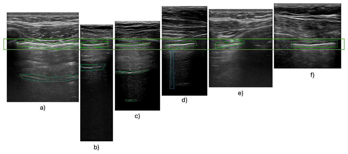
Figure 2: Pleura-aligned images.
Comparison of different types of USG machines with varying footprints and ratios. Images from Hitachi probe: (A), (E); Phillips Lumify probe: (B), (C), (D); SonoScape probe: (F).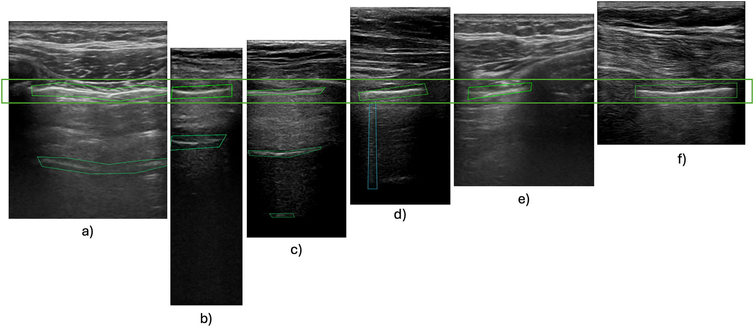
Although such basic resizing might not affect horizontal features, vertical B-lines could be significantly compromised, with the characteristic comet tail shape widened out of proportion. Experimental findings have revealed that incorporating padding during preprocessing leads to improved training outcomes (Alrasheedi, Zhong & Huang, 2023; Tang, Ortis & Battiato, 2019; Haryanto et al., 2020). Our primary experiments also showcased this problem, with our models unable to detect B-lines without the use of padding during training. This limitation persisted when using a small dataset comprising videos with varying size ratios. Incorporating zero padding, a common padding technique, also did not increase the performance of the model. This is caused by artificially introduced zero-value pixels around smaller images, which do not activate during forward or backward propagation, therefore their associated synaptic weights are not modified (Hashemi, 2019). We therefore used edge padding, where the edge pixels (i.e., top/bottom rows and left/right columns) of the original image are repeated in the respective direction (Alrasheedi, Zhong & Huang, 2023).
The final preprocessing pipeline consisted of standardizing resolution to 500 600 pixels, and converting frames to grayscale. No intensity normalisation was performed. This decision was made to retain the raw signal characteristics as output by each machine. Any global normalisation risked introducing artefactual contrasts. Frames were selected using a stratified sampling strategy to balance data across different ultrasound probes and artifact labels. In addition to standard resizing to 500 600, we also tested edge padding that maintains anatomical and artifact structure, which is particularly useful for vertically oriented features. The output data consisted of binary labels indicating the presence or absence of A-lines or B-lines on each annotated frame, used in a supervised classification setting. These labels were generated from medical expert annotations based on the presence of specific polygon types for each artefact.
Augmentation methods
Deep neural networks, mainly CNNs, achieve high performance in various image recognition tasks, yet they often encounter challenges with generalization when trained on limited datasets, leading to overfitting. This issue becomes particularly pronounced in scenarios where data scarcity prevails (Hussain et al., 2017). Augmentation techniques offer a solution to address overfitting by expanding the dataset with additional data points, thereby providing the model with a more diverse set of examples for learning. This approach directly tackles the overfitting problem by enriching the training data and enhancing the model’s capacity to generalize to previously unseen instances (Buslaev et al., 2020).
Augmentation strategies can be divided into two types: augmentation performed on real data and augmentation using synthetically generated data. This article focuses on augmentation techniques applied to an existing dataset.
Affine transformation involves adjusting the geometric properties of images, such as rotation, translation, scaling, and shearing. This technique introduces variations in the spatial orientation of images. Elastic transformation deforms images using spatial deformation fields. Unlike affine transformations, elastic transformations allow for local shape variations without imposing colinearity and aspect ratio constraints. These transformations mimic realistic image variations, thereby contributing to improved model robustness (Nalepa, Marcinkiewicz & Kawulok, 2019). Erasing transformation selectively removes specific regions of an image, replacing them with fixed intensity values or random noise. This approach improves the model’s ability to withstand occlusions and decreases reliance on spurious correlations in the data (Garcea et al., 2023).
We combine different augmentations from these three categories and create a group of augmentations that we call “Basic”, for a full list of the augmentation methods in this group refer to Table 4. These methods are used standardly in most image augmentation solutions, not just for medical data. Other augmentation methods target different characteristics specific to ultrasound data, and were grouped together accordingly. We compared model performance with each augmentation group for benchmarking. All augmentations were applied exclusively to the training subset of each cross-validation fold, while the validation and test subsets remained untouched and contained only the original, radiologist-labelled frames. In every experiment we used the implementations of these augmentation methods from the MONAI open source framework.
| Augmentation set | ||||
|---|---|---|---|---|
| Name of augmentation | Basic (A1) | Without intensity (A2) | Without noise (A3) | All (A4) |
| RandAdjustContrast | x | x | ||
| RandHistogramShift | x | x | ||
| RandBiasField | x | x | ||
| RandFlip | x | x | x | x |
| RandGibbsNoise | x | x | ||
| RandZoom | x | x | x | x |
| RandRotate | x | x | x | x |
| RandGaussianSmooth | x | x | ||
| RandAffine | x | x | x | x |
| RandGridDistortion | x | x | x | x |
| Rand2DElastic | x | x | x | x |
| RandCoarseDropout | x | x | x | x |
| RandGaussianNoise | x | x | ||
We focused our research on pixel-level transformations, which alter pixel values to adjust image characteristics such as brightness, contrast, saturation, and noise. These transformations are particularly useful in grayscale medical imaging modalities, where color-based augmentation is not applicable. Pixel-level transformations aid in standardizing pixel distributions across different imaging protocols, ensuring the model’s robustness to scanner variations (Goceri, 2023).
Various USG machines produce imagery of varying quality and properties–speckle noise, salt and pepper noise, and Gaussian noise are frequent. The most common type of noise is speckle noise, which can have an impact on contrast and other intensity metrics as well as the key visual elements. Sudden image alterations, such as memory cell failure, synchronization errors during digitalization, or incorrect sensor cell activity, might result in the appearance of salt and pepper noise (Vilimek et al., 2022). Electronic circuit noise or sensor noise can cause Gaussian noise. Usually, noise is removed from USG images during preprocessing (Devakumari & Punithavathi, 2020; Nugroho et al., 2016). In contrast, in the second group of augmentation, we tested noise-introducing techniques to let the neural network learn and extract features on noisy images.
In the third group of augmentation methods, we selected techniques that alter image intensity. This was justified as each machine represented in our dataset produces images with different intensities and intensity scales (Stock et al., 2015). Data augmentation serves to improve generalization and robustness of the model. We applied the random bias field augmentation designed for magnetic resonance imaging.
With all augmentation methods, their parameters were set to low values to maintain the most typical characteristics of the frames while also ensuring more robust model training. The parameter values used and their effect were consulted with medical experts and were aligned with variance that can occur during standard examinations (e.g., for rotation, we used angles that replicate the examiner moving the probe into different angles).
Experiments and results
In this section we present the results of our evaluation of different standard approaches used for increasing model performance. We first look at the difference in performance when using historical data for amending an existing dataset, then turn our attention to exploring the effect of using preprocessing techniques resize and spatial padding, and then conclude by discussing how combinations of different augmentation methods influence model performance.
For each experiment, we provide the average F1-score, the negative predictive value (NPV), and true positive rate (TPR) over 5-fold cross-validation, along with the standard deviation. Negative predictive value was chosen for its relevance in real-life use cases, as we want to limit the number of false negatives as much as possible. True positive rate was selected for a similar reason, with the correct detection of artifacts being of crucial importance in deployment. A graphical overview of the effect of various approaches on the F1-score is presented in Fig. 3 with changes compared to benchmark settings (original dataset, image resizing, no augmentation) shown.
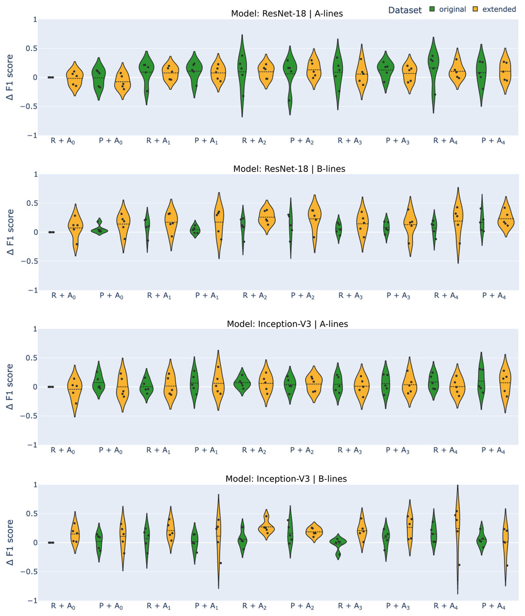
Figure 3: Differential F1-scores ( -score) for A-line and B-line detection using ResNet-18 and Inception-V3 models with original (green) and extended (orange) datasets across various augmentation methods.
R–reshape; P–edge padding. All results are benchmarked to model.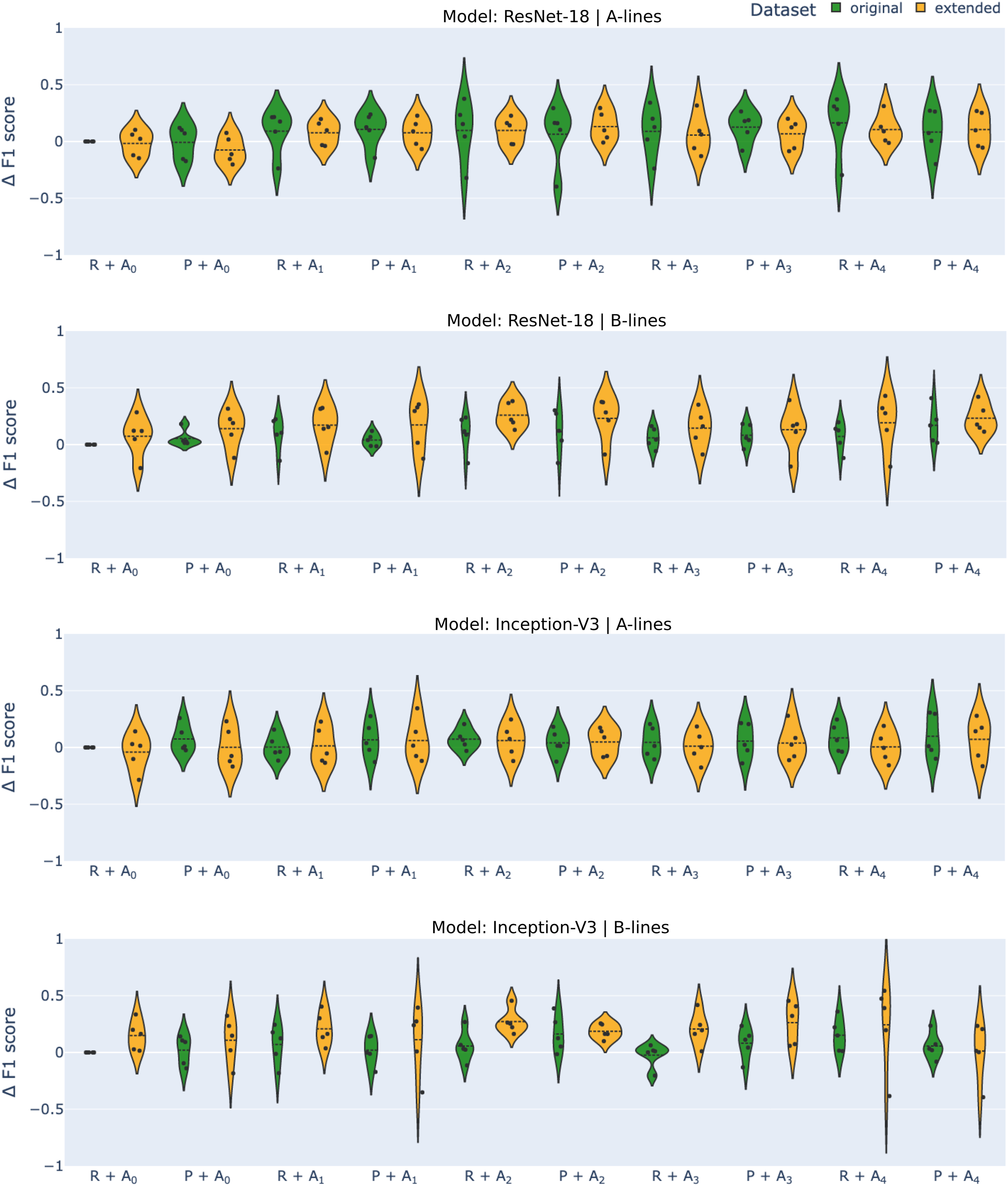
Datasets
In our initial experiment, we set out to test the hypothesis that extending the original dataset with historical data, specifically videos of examinations done with other ultrasound probes, would enhance the model’s generalization ability and overall performance. The results, as shown in Table 5, reveal that the model’s performance on A- and B-line detection tasks varied when trained on the original dataset (consisting of only footages taken with Lumify probe) and the extended dataset, contradicting our initial assumption.
| Task | Model | Dataset | F1 | TPR | NPV | |||
|---|---|---|---|---|---|---|---|---|
| Mean | Std | Mean | Std | Mean | Std | |||
| A-lines | Inception-v3 | Original | 0.734 | 0.083 | 0.686 | 0.223 | 0.824 | 0.118 |
| Extended | 0.693 | 0.125 | 0.658 | 0.237 | 0.778 | 0.168 | ||
| ResNet-18 | Original | 0.691 | 0.149 | 0.696 | 0.226 | 0.824 | 0.083 | |
| Extended | 0.675 | 0.105 | 0.561 | 0.239 | 0.751 | 0.157 | ||
| B-lines | Inception-v3 | Original | 0.531 | 0.189 | 0.196 | 0.243 | 0.866 | 0.02 |
| Extended | 0.679 | 0.187 | 0.534 | 0.285 | 0.91 | 0.056 | ||
| ResNet-18 | Original | 0.473 | 0.121 | 0.082 | 0.13 | 0.846 | 0.044 | |
| Extended | 0.546 | 0.112 | 0.329 | 0.173 | 0.888 | 0.06 | ||
The observed results can be attributed to the nature of A-lines and B-lines in the dataset. A-lines were present in a majority of frames, visible in approximately 67% of the annotated frames, whereas B-lines appeared in only about 29% of labeled frames (see Tables 1, 2, 3). This means that B-lines were particularly underrepresented in the annotated data, leading to significant performance improvements when additional training data was introduced. The lack of difference in the effect on the two different models suggests that the dataset extension had a similar impact on both. The most significant increase in performance was seen in TPR for B-lines, with the value rising from 0.196 to 0.534 for Inception-v3 and from 0.082 to 0.329 for ResNet-18. However, it’s important to note that extending the dataset also increased the standard deviation for both NPV and TPR metrics for both tasks and models. This can be attributed to the higher variance in data, which made model performance more sensitive to train-test splits during cross-validation.
Transformation methods
Tables 6 and 7 show the results of training when different transformation methods were used for A- and B-line detection, respectively. For the former, the effect of using edge padding instead of the standard resize for transformation was inconclusive. The values of metrics we considered were somewhat worse for ResNet-18, although these changes were small, around 0.05. A bigger change was only registered for TPR when using the extended dataset. However, when using the original dataset, the standard deviation got significantly smaller, from 0.226 to 0.097, when using edge padding. There was some improvement in the metrics with the Inception-v3 network. F1-score and negative predictive value increased in all setups, while the true positive rate decreased for the original dataset from 0.824 to 0.728. No significant changes in standard deviation were observed, except for NPV on data from the original dataset, where the standard deviation was more than halved.
| Model | Dataset | Transformation | F1 | TPR | NPV | |||
|---|---|---|---|---|---|---|---|---|
| Mean | Std | Mean | Std | Mean | Std | |||
| Inception-v3 | Original | Resize | 0.734 | 0.083 | 0.685 | 0.223 | 0.824 | 0.118 |
| Padding | 0.808 | 0.083 | 0.728 | 0.193 | 0.847 | 0.106 | ||
| Extended | Resize | 0.693 | 0.125 | 0.658 | 0.237 | 0.778 | 0.168 | |
| Padding | 0.735 | 0.129 | 0.675 | 0.263 | 0.808 | 0.186 | ||
| ResNet-18 | Original | Resize | 0.691 | 0.149 | 0.696 | 0.226 | 0.824 | 0.083 |
| Padding | 0.684 | 0.139 | 0.653 | 0.097 | 0.771 | 0.087 | ||
| Extended | Resize | 0.675 | 0.105 | 0.561 | 0.239 | 0.751 | 0.157 | |
| Padding | 0.617 | 0.137 | 0.465 | 0.206 | 0.701 | 0.161 | ||
| Model | Dataset | Transformation | F1 | TPR | NPV | |||
|---|---|---|---|---|---|---|---|---|
| Mean | Std | Mean | Std | Mean | Std | |||
| Inception-v3 | Original | Resize | 0.531 | 0.189 | 0.196 | 0.242 | 0.866 | 0.02 |
| Padding | 0.552 | 0.108 | 0.254 | 0.254 | 0.88 | 0.026 | ||
| Extended | Resize | 0.679 | 0.187 | 0.534 | 0.285 | 0.91 | 0.056 | |
| Padding | 0.639 | 0.185 | 0.551 | 0.256 | 0.902 | 0.062 | ||
| ResNet-18 | Original | Resize | 0.473 | 0.121 | 0.082 | 0.13 | 0.846 | 0.043 |
| Padding | 0.527 | 0.188 | 0.215 | 0.253 | 0.869 | 0.043 | ||
| Extended | Resize | 0.546 | 0.112 | 0.329 | 0.173 | 0.888 | 0.06 | |
| Padding | 0.613 | 0.123 | 0.403 | 0.141 | 0.904 | 0.048 | ||
For B-line detection, we observed a generally positive effect of using edge padding. Although changes were not high in F1-score and NPV, there was an apparent increase in TPR for ResNet when using only the original dataset, with recall increasing from 0.082 to 0.215. Performance dropped only when training Inception-v3 on the extended dataset, with a decrease of 0.04 in F1-score and a slight decrease in NPV, while TPR increased even in this case. Overall, the results suggest that using edge padding instead of resizing leads to improved performance for B-line detection.
Another indication of improvement is observed in the saliency maps (Fig. 4): with edge padding, activation is clearly concentrated in the regions where B-lines occur and does not migrate to the padded borders. In contrast, resizing does not highlight B-line regions: in the top example it produces a small line-like patch unrelated to the pleural tract, and in the bottom example the activation is diffuse and off-target. For A-lines (Fig. 5), saliency overlays are less focal than for B-lines: activation spreads along and below the pleura and is often diffuse, offering weaker discriminative guidance. This qualitative pattern aligns with the systematic performance drop we observed with padding for A-lines (Table 6). This pattern was observed consistently across folds and devices in our dataset. Representative failures are shown in Fig. 6: the first row illustrates an A-line case where resizing outperforms padding, and the second row shows a B-line case where both preprocessing choices yield poor focus and predictions.
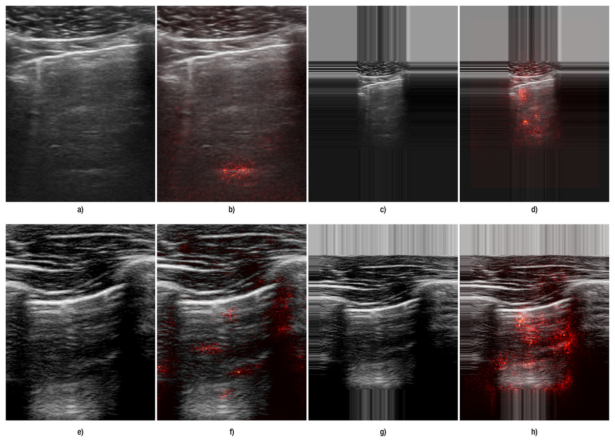
Figure 4: Comparison of the effect of data transformation on lung ultrasound images for B-lines.
(A–D) correspond to images from Hitachi device, and (E–H) correspond to those from the Sonoscape device. Panels (A, E) show the original images preprocessed by resizing, while panels (C, G) show the original images preprocessed with edge padding. Panels (B, F) and (D, H) present the corresponding saliency map overlays for the resize and edge-padding methods, respectively.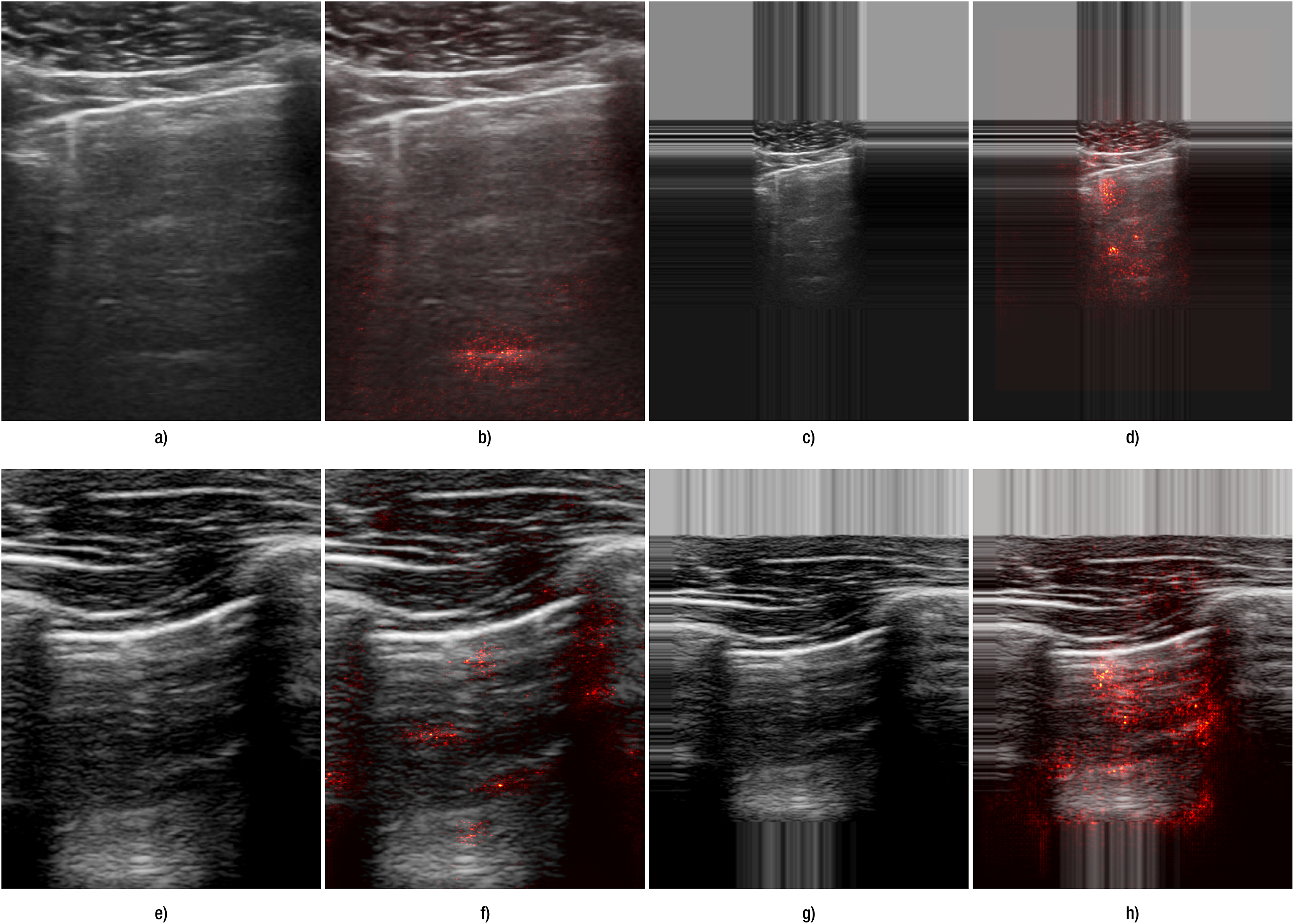
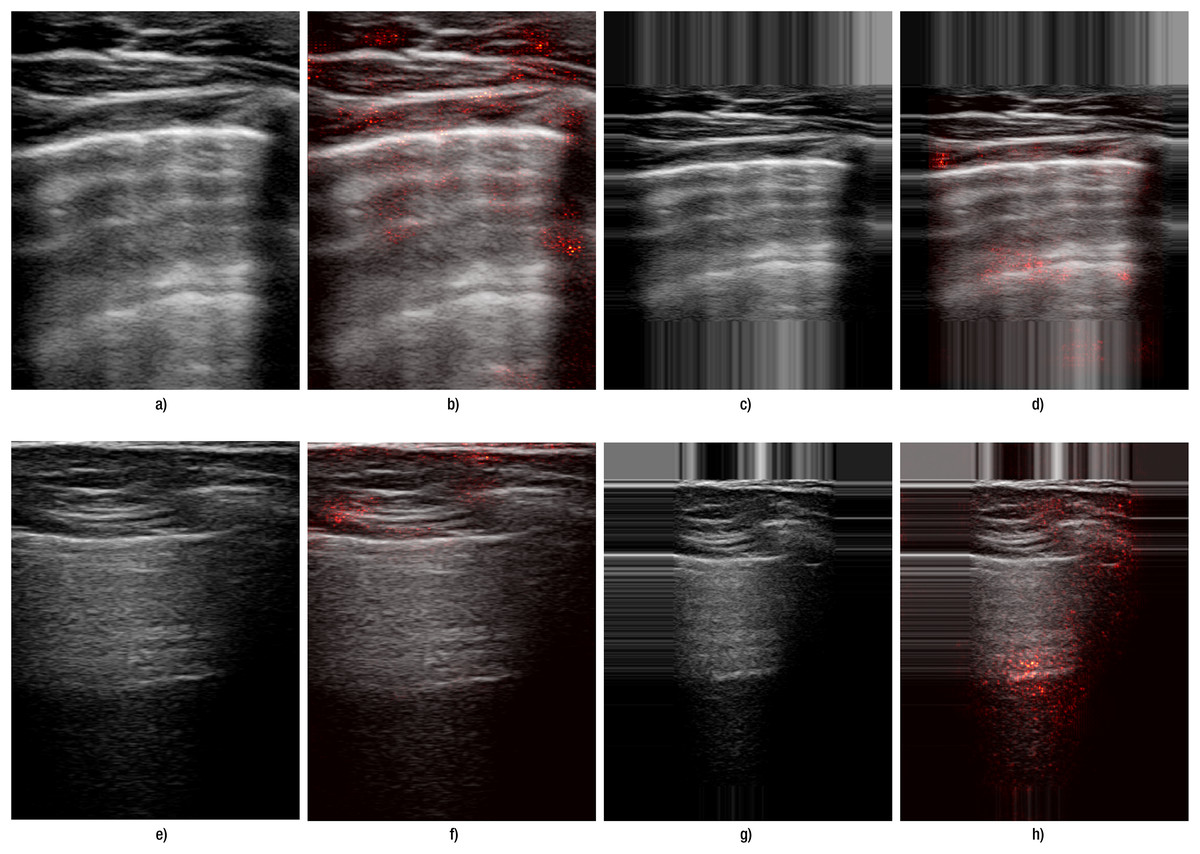
Figure 5: Comparison of the effect of data transformation on lung ultrasound images for A-lines.
(A–D) correspond to images from Lumify device, and (E–H) correspond to Sonoscape device. (A, E) show the original images preprocessed by resizing, while (C, G) show the original images preprocessed with edge padding. (B, F) and (D, H) present the corresponding saliency map overlays for the resize and edge-padding methods, respectively.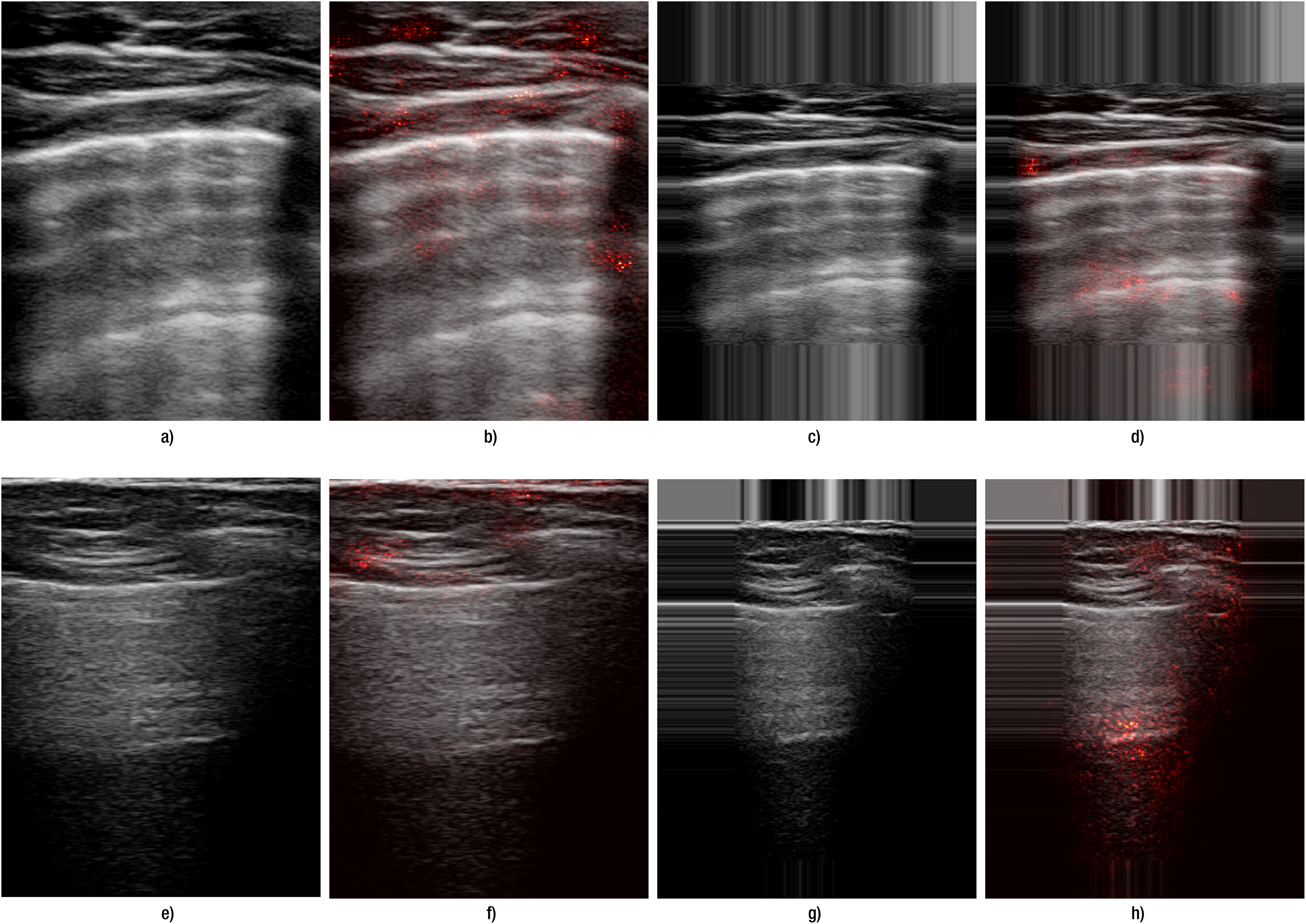
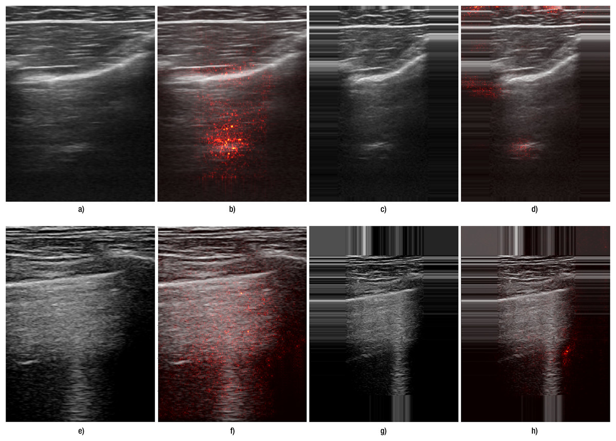
Figure 6: Failure cases for both A- and B-lines.
(A–D) correspond to images from Hitachi devices with A-lines; (E–H) correspond to Lumify device with B-lines. (A, E) show the original images preprocessed by resizing, while (C, G) show the original images preprocessed with edge padding. (B, F) and (D, H) present the corresponding saliency map overlays for the resize and edge-padding methods, respectively.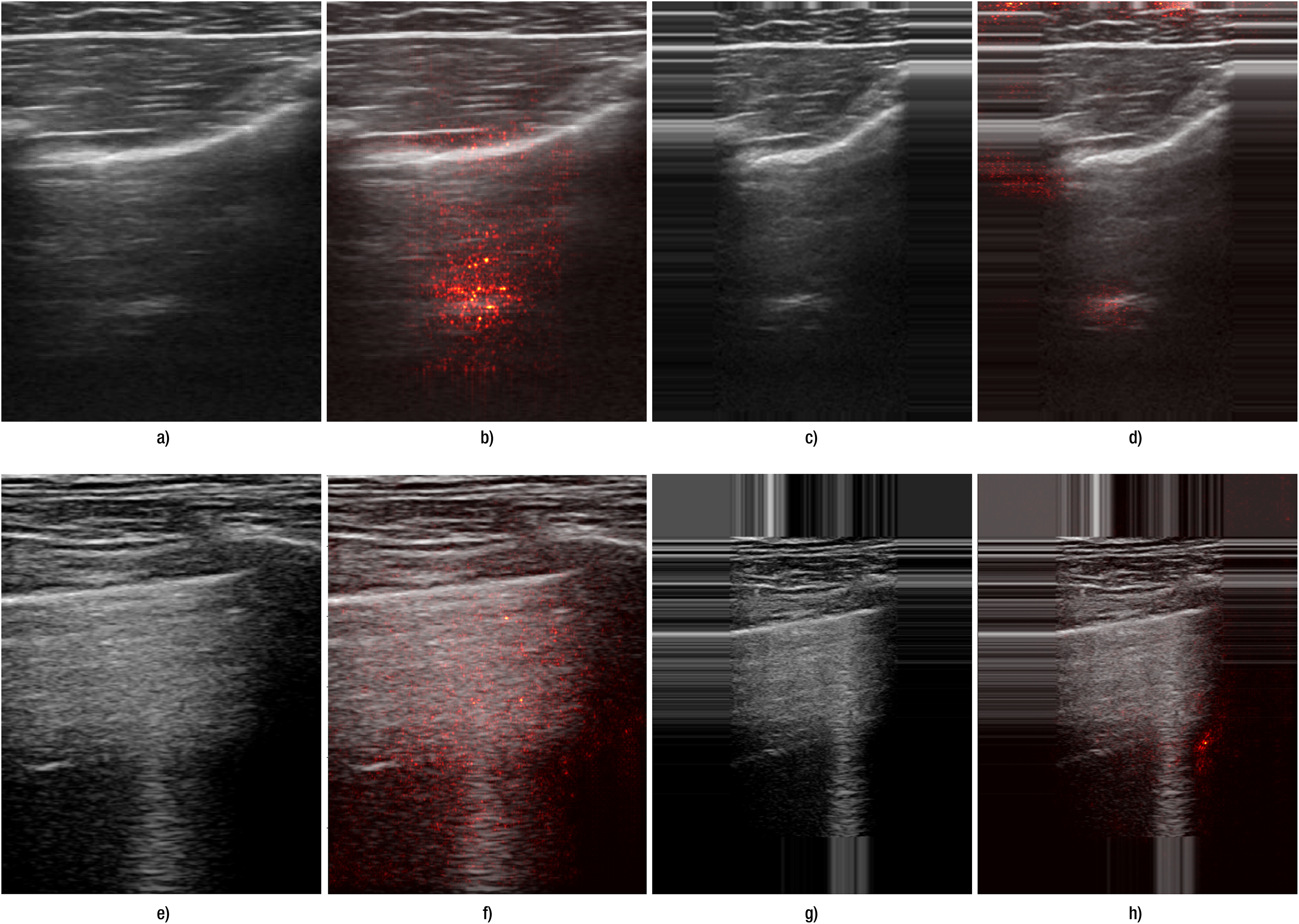
The results were in accordance with our hypothesis that, as B-lines represent vertical features that could be distorted by standard resizing, carefully selected transformation and preprocessing methods can greatly influence final performance. When we juxtapose the results obtained using resizing and edge padding, we see that even for A-line detection, performance remained at least on a comparable level.
Augmentation methods
Our final experiments explored the changes in performance metrics for training models when using various combinations of augmentation methods on both the original and the extended dataset. We expected a high variability depending on what augmentation methods were used, and results presented in Tables 8 through 11 support this presumption.
| F1 | TPR | NPV | ||||||
|---|---|---|---|---|---|---|---|---|
| Dataset | Transformation | Augmentation | Mean | Std | Mean | Std | Mean | Std |
| Original | Resize | A0 | 0.734 | 0.083 | 0.685 | 0.223 | 0.824 | 0.118 |
| A1 | 0.736 | 0.06 | 0.636 | 0.141 | 0.793 | 0.085 | ||
| A2 | 0.779 | 0.079 | 0.66 | 0.118 | 0.809 | 0.1 | ||
| A3 | 0.806 | 0.087 | 0.781 | 0.162 | 0.87 | 0.114 | ||
| A4 | 0.817 | 0.074 | 0.834 | 0.166 | 0.894 | 0.125 | ||
| Padding | A0 | 0.808 | 0.083 | 0.728 | 0.193 | 0.847 | 0.106 | |
| A1 | 0.801 | 0.125 | 0.791 | 0.152 | 0.858 | 0.14 | ||
| A2 | 0.789 | 0.078 | 0.752 | 0.137 | 0.851 | 0.097 | ||
| A3 | 0.774 | 0.038 | 0.578 | 0.092 | 0.785 | 0.082 | ||
| A4 | 0.832 | 0.114 | 0.836 | 0.132 | 0.885 | 0.106 | ||
| Extended | Resize | A0 | 0.693 | 0.125 | 0.658 | 0.237 | 0.778 | 0.168 |
| A1 | 0.748 | 0.121 | 0.653 | 0.252 | 0.799 | 0.176 | ||
| A2 | 0.744 | 0.111 | 0.705 | 0.263 | 0.832 | 0.172 | ||
| A3 | 0.795 | 0.08 | 0.72 | 0.213 | 0.833 | 0.154 | ||
| A4 | 0.738 | 0.115 | 0.671 | 0.195 | 0.79 | 0.165 | ||
| Padding | A0 | 0.735 | 0.129 | 0.675 | 0.263 | 0.808 | 0.186 | |
| A1 | 0.795 | 0.126 | 0.789 | 0.208 | 0.858 | 0.184 | ||
| A2 | 0.773 | 0.116 | 0.71 | 0.278 | 0.839 | 0.176 | ||
| A3 | 0.783 | 0.072 | 0.714 | 0.213 | 0.838 | 0.169 | ||
| A4 | 0.806 | 0.109 | 0.713 | 0.244 | 0.837 | 0.174 | ||
| F1 | TPR | NPV | ||||||
|---|---|---|---|---|---|---|---|---|
| Dataset | Transformation | Augmentation | Mean | Std | Mean | Std | Mean | Std |
| Original | Resize | A0 | 0.691 | 0.149 | 0.696 | 0.226 | 0.824 | 0.083 |
| A1 | 0.782 | 0.053 | 0.744 | 0.136 | 0.834 | 0.121 | ||
| A2 | 0.781 | 0.106 | 0.727 | 0.212 | 0.829 | 0.15 | ||
| A3 | 0.789 | 0.135 | 0.794 | 0.134 | 0.851 | 0.127 | ||
| A4 | 0.856 | 0.127 | 0.856 | 0.17 | 0.898 | 0.145 | ||
| Padding | A0 | 0.684 | 0.139 | 0.653 | 0.097 | 0.771 | 0.087 | |
| A1 | 0.798 | 0.066 | 0.697 | 0.159 | 0.831 | 0.072 | ||
| A2 | 0.818 | 0.061 | 0.803 | 0.113 | 0.876 | 0.082 | ||
| A3 | 0.756 | 0.136 | 0.722 | 0.242 | 0.87 | 0.112 | ||
| A4 | 0.774 | 0.114 | 0.738 | 0.147 | 0.827 | 0.112 | ||
| Extended | Resize | A0 | 0.675 | 0.105 | 0.561 | 0.239 | 0.751 | 0.157 |
| A1 | 0.768 | 0.118 | 0.684 | 0.251 | 0.817 | 0.164 | ||
| A2 | 0.748 | 0.149 | 0.67 | 0.291 | 0.818 | 0.19 | ||
| A3 | 0.788 | 0.12 | 0.676 | 0.219 | 0.814 | 0.143 | ||
| A4 | 0.797 | 0.15 | 0.734 | 0.206 | 0.833 | 0.161 | ||
| Padding | A0 | 0.616 | 0.137 | 0.465 | 0.206 | 0.701 | 0.161 | |
| A1 | 0.768 | 0.142 | 0.665 | 0.222 | 0.806 | 0.16 | ||
| A2 | 0.758 | 0.113 | 0.637 | 0.223 | 0.796 | 0.148 | ||
| A3 | 0.823 | 0.125 | 0.745 | 0.215 | 0.848 | 0.175 | ||
| A4 | 0.796 | 0.143 | 0.731 | 0.198 | 0.835 | 0.169 | ||
| F1 | TPR | NPV | ||||||
|---|---|---|---|---|---|---|---|---|
| Dataset | Transformation | Augmentation | Mean | Std | Mean | Std | Mean | Std |
| Original | Resize | A0 | 0.531 | 0.189 | 0.196 | 0.243 | 0.866 | 0.02 |
| A1 | 0.601 | 0.158 | 0.435 | 0.198 | 0.894 | 0.03 | ||
| A2 | 0.508 | 0.12 | 0.353 | 0.232 | 0.875 | 0.015 | ||
| A3 | 0.586 | 0.145 | 0.43 | 0.211 | 0.895 | 0.032 | ||
| A4 | 0.683 | 0.214 | 0.566 | 0.251 | 0.925 | 0.03 | ||
| Padding | A0 | 0.552 | 0.108 | 0.254 | 0.254 | 0.88 | 0.026 | |
| A1 | 0.551 | 0.114 | 0.253 | 0.214 | 0.877 | 0.021 | ||
| A2 | 0.612 | 0.155 | 0.34 | 0.216 | 0.892 | 0.01 | ||
| A3 | 0.694 | 0.218 | 0.588 | 0.247 | 0.929 | 0.03 | ||
| A4 | 0.587 | 0.175 | 0.397 | 0.203 | 0.89 | 0.02 | ||
| Extended | Resize | A0 | 0.679 | 0.187 | 0.534 | 0.285 | 0.91 | 0.056 |
| A1 | 0.739 | 0.162 | 0.626 | 0.257 | 0.93 | 0.046 | ||
| A2 | 0.737 | 0.175 | 0.589 | 0.249 | 0.922 | 0.052 | ||
| A3 | 0.802 | 0.117 | 0.737 | 0.199 | 0.953 | 0.031 | ||
| A4 | 0.775 | 0.206 | 0.683 | 0.225 | 0.94 | 0.041 | ||
| Padding | A0 | 0.639 | 0.185 | 0.551 | 0.256 | 0.902 | 0.062 | |
| A1 | 0.644 | 0.132 | 0.361 | 0.232 | 0.913 | 0.036 | ||
| A2 | 0.794 | 0.125 | 0.618 | 0.295 | 0.938 | 0.039 | ||
| A3 | 0.717 | 0.178 | 0.494 | 0.306 | 0.909 | 0.063 | ||
| A4 | 0.543 | 0.07 | 0.5 | 0.238 | 0.909 | 0.059 | ||
| F1 | TPR | NPV | ||||||
|---|---|---|---|---|---|---|---|---|
| Dataset | Transformation | Augmentation | Mean | Std | Mean | Std | Mean | Std |
| Original | Resize | A0 | 0.473 | 0.121 | 0.082 | 0.13 | 0.846 | 0.044 |
| A1 | 0.569 | 0.214 | 0.261 | 0.268 | 0.875 | 0.039 | ||
| A2 | 0.532 | 0.121 | 0.349 | 0.333 | 0.889 | 0.04 | ||
| A3 | 0.572 | 0.219 | 0.316 | 0.342 | 0.886 | 0.045 | ||
| A4 | 0.545 | 0.173 | 0.365 | 0.362 | 0.895 | 0.044 | ||
| Padding | A0 | 0.527 | 0.188 | 0.215 | 0.253 | 0.869 | 0.043 | |
| A1 | 0.513 | 0.099 | 0.264 | 0.214 | 0.869 | 0.021 | ||
| A2 | 0.556 | 0.126 | 0.457 | 0.337 | 0.903 | 0.048 | ||
| A3 | 0.587 | 0.175 | 0.409 | 0.312 | 0.894 | 0.039 | ||
| A4 | 0.643 | 0.171 | 0.367 | 0.252 | 0.899 | 0.041 | ||
| Extended | Resize | A0 | 0.546 | 0.112 | 0.329 | 0.173 | 0.888 | 0.06 |
| A1 | 0.645 | 0.17 | 0.369 | 0.197 | 0.888 | 0.091 | ||
| A2 | 0.618 | 0.118 | 0.461 | 0.346 | 0.903 | 0.069 | ||
| A3 | 0.731 | 0.165 | 0.686 | 0.091 | 0.941 | 0.036 | ||
| A4 | 0.665 | 0.179 | 0.538 | 0.314 | 0.938 | 0.024 | ||
| Padding | A0 | 0.613 | 0.123 | 0.403 | 0.141 | 0.904 | 0.048 | |
| A1 | 0.647 | 0.139 | 0.532 | 0.4 | 0.923 | 0.065 | ||
| A2 | 0.604 | 0.139 | 0.543 | 0.327 | 0.914 | 0.063 | ||
| A3 | 0.705 | 0.087 | 0.73 | 0.186 | 0.95 | 0.032 | ||
| A4 | 0.705 | 0.161 | 0.633 | 0.279 | 0.927 | 0.058 | ||
Considering A-line detection with Inception-v3 (Table 8), we observe a mixed augmentation effect on various metrics. Combining all augmentation methods listed in Table 4 resulted in the best performance when using the original dataset. This constitutes a 10 percent increase in F1-score with the original dataset with resizing (from 0.734 to 0.817), and an increase of 0.03 when using padding. Similar increases can be observed when training on the extended dataset (an increase of 0.04 and 0.07, respectively). The most notable difference was in NPV with all augmentation methods used, the value increasing from 0.685 to 0.834, a 0.15 increase. On the other hand, somewhat surprisingly, other combinations of augmentation methods caused a decrease in the F1-score when using padding, and a negative effect could be seen in the other two metrics with resizing.
A more generally positive effect of augmentation was observed when training on the extended dataset. Values of the selected metrics increased in almost all cases, except for TPR when using resize and only basic augmentation methods; the value was, however, still comparable to when no augmentation was used. The best F1-scores were around 0.8, although this could be achieved with different combinations of augmentation methods. When using resize, the combination with no noises proved to be the best, while with padding, a combination of all considered augmentation methods did. This might be due to padding repeating values from the edges of the images, which disrupts data distribution, which in turn can be mitigated by introducing noise. However, when using resize, this is not such a big issue since simple resizing maintains the noise characteristics of the original frames. This trend could also be observed in original data when leaving out noises, which resulted in results comparable to the best improvement when using resize. However, it is important to note that since extending the dataset did not have a largely positive effect on A-line detection, data augmentation did not increase relevant metrics significantly compared to the benchmark model (original dataset, resize, and no augmentation). Improvements were negligible for NPV, they moved around 0.02 for TPR and 0.07 for F1-score.
A generally positive augmentation effect was observed when training ResNet-18 (Table 9), both on the original and the extended dataset, with the improvements being higher than in the case of Inception-v3. With the original dataset, when using resize, applying all augmentation methods we considered proved to be the most suitable, raising the F1-score from 0.691 to 0.856, an increase of 0.165. When using edge padding, augmentations without intensity were the best, resulting in an F1-score of 0.818 (compared to a 0.684 benchmark). These combinations had the highest impacts on TPR and NPV, as well.
For training on the extended dataset, applying all augmentation methods caused the biggest improvement in combination with resize and augmentation methods without noise when using edge padding. This corresponds to the results obtained for training Inception-v3. There was a significant improvement in the F1-score from 0.675 to 0.797 and from 0.616 to 0.823 with resize and padding, respectively. NPV also increased from 0.751 to 0.833 and from 0.701 to 0.848. The biggest improvement was observed for recall, which increased from 0.561 to 0.734 and from 0.465 to 0.745, respectively. Of all experiments, we achieved at most a 0.16 increase in F1-score and TPR and 0.07 in NPV compared to the benchmark (original dataset, resize, no augmentation used).
B-line detection showed poorer results when no augmentation was used, and especially recall remained low for both models. All data augmentation combinations showed a positive effect, as can be seen in Tables 10 and 11, but for a few exceptions. The combinations that worked best were similar to those determined with A-line detection, namely all augmentation methods and augmentation without the introduction of noise.
For the Inception-v3 model with the original dataset, all augmentations improved all metrics most when combined with resize. F1-score increased from 0.531 to 0.683, NPV from 0.866 to 0.925. The biggest increase was observed for TPR, which changed from 0.196 to 0.566 thanks to introducing augmentation to the training process. Leaving out noise helped when using edge padding, with F1-score reaching 0.694, TPR at 0.588, and NPV at 0.929. A combination of only basic augmentation methods led to a decrease in all considered metrics. When training on the extended dataset, augmentation without noise worked best with resize, and augmentation without intensity led to the highest increase in performance with edge padding. F1-score was around 0.8 in both cases, which constitutes the highest value achieved for B-line detection. This represents a notable improvement compared to the benchmark model, which had an F1-score of 0.531. Best recall and NPV were achieved with the extended dataset and augmentation without noise, at 0.737 and 0.953, respectively.
Augmentation had a positive effect on training ResNet-18 for B-line detection as well, with both datasets. On the original dataset with resize, there was an increase of 0.1 in F1-score when data augmentation without noise was used (0.572 compared with 0.473), however, TPR and NPV were the highest when a combination of all augmentation methods was used. The increase was most significant with recall, with the value reaching 0.365 with augmentation compared to 0.082. With edge padding, a combination of all augmentation methods led to the best F1-score with 0.643 (up from 0.527), while other metrics reached their highest value with augmentation without noise. Recall once again more than doubled from 0.215 to 0.457.
On the extended dataset, augmentation without noise worked best in both test scenarios with different image transformations. When combined with resize, F1-score reached 0.731 (largest overall with ResNet-18 for B-line detection), TPR was at 0.686 (up from 0.329), and NPV at 0.941. With edge padding, F1-score was at 0.705, TPR at 0.73, and NPV at 0.95, the latter two constituting the best results obtained with ResNet-18 for the given task. F1-score was similarly at 0.705 when all augmentation methods were used, but the other two metrics were lower with 0.633 and 0.927, respectively.
Discussion
Data augmentation has proven beneficial for lung ultrasound tasks, where training data are often sparse. Recent studies confirm that augmenting limited datasets significantly improves model generalisation and robustness. For instance, Zhao, Fong & Bell (2024) reported a 165% increase in Dice score (from 0.17 to 0.45) for B-line segmentation when augmentation was applied. An extensive review of augmentation methods in medical imaging—covering diverse modalities and anatomical targets—can be found in Goceri (2023), who outlines how augmentation helps mitigate overfitting and enhances feature representation in small and imbalanced datasets.
We evaluate frame-level A- and B-lines detection with ResNet-18 and Inception-v3 using 5-fold cross-validation and report F1-score, NPV, and TPR (mean SD). We used saliency overlays as qualitative illustrations of model focus under different preprocessing choices (resize vs. edge padding) and are not used as decision criteria.
Our findings support these results: augmentation notably improved both A-line and B-line detection. In our experiments, B-line recall increased from 0.2 to 0.7 for Inception-v3 and from 0.08 to 0.7 for ResNet-18. Corresponding F1-scores rose to 0.80 and 0.70, respectively. A-line detection also showed strong gains, with F1-scores rising to 0.83 for Inception-v3 and 0.86 for ResNet-18. The highest true positive rates were achieved by ResNet-18 for A-lines (0.86) and by Inception-v3 for B-lines (0.74), while Inception-v3 also attained the best negative predictive values: 0.89 for A-lines and 0.95 for B-lines.
These results support our hypothesis that both preprocessing and augmentation—especially spatial padding and noise-free transformations—are essential for preserving diagnostically significant features such as B-lines. These vertical structures are particularly susceptible to distortion under standard resizing, as evidenced by the saliency maps, where models trained with edge-padded inputs more effectively attended to the correct regions.
Importantly, this study suggests that frame-level classification may serve as a viable and lightweight alternative to pixel-level segmentation, especially in resource-constrained environments. In contrast to recent segmentation-based approaches by Xing et al. (2023, 2024), Howell et al. (2024), and Lucassen et al. (2023), which require densely labeled datasets and more complex architectures, our method achieves competitive results using sparse frame-level annotations. This approach is thus well-suited for deployment in clinical settings where labeling resources are limited and model simplicity is a practical advantage.
In terms of architecture, we selected ResNet-18 and Inception-v3 based on their balance between performance and computational efficiency. Here, computational efficiency refers to model compactness and training simplicity rather than measured inference speed or memory. In additional experiments (not detailed in the manuscript), we also trained deeper ResNet variants (e.g., ResNet-34, ResNet-50). Although these deeper models showed improvements in F1-score, they were more prone to overfitting due to the dataset’s limited size and did not consistently outperform the simpler architectures. These findings support the use of lightweight models in scenarios with constrained training data.
For future research, we plan to explore other architectures such as EfficientNetV2, ConvNeXt, or MobileNetV3, which offer improved performance-efficiency trade-offs. DenseNet may also provide benefits through enhanced feature reuse. Additionally, we aim to address the challenges of sparse labeling through generative augmentation techniques and reinforcement learning strategies. Beyond classification, we will evaluate how these data handling techniques impact segmentation performance on LUS data.
Conclusion
This study demonstrates that accurate detection of A-line and B-line artifacts in lung ultrasound is achievable even with sparse annotations, using a combination of appropriate preprocessing and targeted augmentation. The most notable gains were observed in B-line detection, where recall improved from 0.2 to 0.7 for Inception-v3, and from 0.08 to 0.7 for ResNet-18, following the use of augmentation and additional probe-derived data. A-line detection also performed strongly, reaching F1-scores of 0.83 and 0.86 for Inception-v3 and ResNet-18, respectively.
Edge-aware padding proved particularly beneficial in preserving vertical structures like B-lines, confirming the importance of artifact-specific preprocessing. Furthermore, both models—despite their simplicity—achieved competitive results, highlighting the viability of lightweight architectures for real-world deployment in data-limited clinical environments.
Overall, our findings suggest that robust LUS artifact detection does not require complex models or dense annotations. Instead, careful data curation and preprocessing are sufficient to build effective, scalable AI tools for bedside diagnostic support.