Efficient Parkinson’s disease classification from speech with filter-based feature selection and Genetic Algorithm–Bayesian Optimization ensemble integration

Hakan Gunduz

doi:10.7717/peerj-cs.3430

Efficient Parkinson’s disease classification from speech with filter-based feature selection and Genetic Algorithm–Bayesian Optimization ensemble integration

Hakan Gunduz

Software Engineering Department, Kocaeli University, Kocaeli, Turkey

DOI: 10.7717/peerj-cs.3430

Published: 2025-12-09
Accepted: 2025-11-06
Received: 2025-07-04

Academic Editor: Nicole Nogoy

Subject Areas: Artificial Intelligence, Computer Education, Data Mining and Machine Learning, Neural Networks
Keywords: Hybrid filter-based selection, Iterative majority voting ensemble, GA–BO ensemble voting, Parkinson’s disease classification

Copyright: © 2025 Gunduz
Licence: This is an open access article distributed under the terms of the Creative Commons Attribution License, which permits unrestricted use, distribution, reproduction and adaptation in any medium and for any purpose provided that it is properly attributed. For attribution, the original author(s), title, publication source (PeerJ Computer Science) and either DOI or URL of the article must be cited.

Cite this article: Gunduz H. 2025. Efficient Parkinson’s disease classification from speech with filter-based feature selection and Genetic Algorithm–Bayesian Optimization ensemble integration. PeerJ Computer Science 11:e3430 https://doi.org/10.7717/peerj-cs.3430

The author has chosen to make the review history of this article public.

Abstract

Parkinson’s disease (PD) is a progressive neurodegenerative disorder of the central nervous system that significantly impairs quality of life. Early and accurate diagnosis is essential to improve treatment outcomes and slow disease progression. In this study, we propose a computationally efficient and clinically feasible framework for PD classification based solely on vocal biomarkers. Our method leverages selective feature optimization and lightweight ensemble learning, avoiding reliance on deep or computationally intensive architectures. Three ensemble strategies are evaluated: (i) iterative majority voting, (ii) Genetic Algorithm (GA)-based classifier selection, and (iii) Bayesian Optimization (BO)-based probabilistic weighting. Building on these, we introduce a hybrid GA–BO ensemble method that combines GA-driven model selection with BO-guided weighting to optimize diagnostic performance. Experimental results demonstrate that the hybrid ensemble achieves state-of-the-art metrics, including 96.4% accuracy, 97.6% F1-score, and a Matthews Correlation Coefficient (MCC) of 0.906. The proposed system is adaptable across diverse feature sets and suitable for integration into mobile or edge-computing platforms. Overall, the framework offers a non-invasive, scalable, and cost-effective decision support tool for early-stage PD diagnosis.

Introduction

Parkinson’s disease (PD) is a progressive neurodegenerative disease that affects the central nervous system. The primary feature of PD is the reduction of dopamine levels in the substantia nigra, a part of the brain critical for movement coordination (Massano & Bhatia, 2012). Dopamine is essential to ensure smooth and precise motor movements; therefore, its insufficiency results in motor problems, including tremors (Tysnes & Storstein, 2017), muscle stiffness (Raiano et al., 2020), reduced movement ability (Jankovic, 2008), and walking difficulties (Palakurthi & Burugupally, 2019). Additional symptoms can include fatigue, disturbances in sleep, cognitive challenges, and depression (Goldman et al., 2018). Importantly, speech impairments often serve as early indicators of PD (Goberman, Blomgren & Metzger, 2010; Tolosa et al., 2021).

The exact cause of PD is not fully understood, as it is believed to arise from a combination of genetic and environmental factors. Although there is currently no cure, treatments that involve medication, surgery, and physical therapy can help manage symptoms. The condition is generally more common in those over 60 years of age and marginally more widespread in men, but younger adults can also be affected (Stoker & Barker, 2020).

Alterations in speech, such as diminished vocal clarity, monotonic intonation, and hoarseness, frequently occur before motor symptoms, rendering speech-based diagnostics a promising path (Gunduz, 2019; Karaman et al., 2021; Quan et al., 2022). Despite this, diagnosing early on poses difficulties due to the requirement for clinical expertise, which may be scarce in low-resource regions. This has motivated the development of computer-aided diagnosis (CAD) systems to aid clinicians, reduce diagnostic errors, and enhance scalability.

Earlier studies have investigated various modalities for PD diagnosis, including electroencephalogram (EEG) (Li et al., 2024), magnetic resonance imaging (MRI) (Rana et al., 2017), Gamma scans (Tassew, Xuan & Chai, 2023), handwriting analysis (Diaz et al., 2019; Islam et al., 2024), and gait freezing patterns (El Maachi, Bilodeau & Bouachir, 2020). Among these, speech-based detection has emerged as particularly effective due to its non-invasive and cost-efficient nature (Moro-Velazquez et al., 2021; Jeancolas et al., 2021). Accordingly, a wide range of machine learning (ML) and deep learning (DL) methods have been proposed. Classical ML approaches, including support vector machines (SVMs) (Gunduz, 2019, 2021), boosting algorithms (Lamba, Gulati & Jain, 2022), and meta-heuristics such as Minimum Redundancy Maximum Relevance (mRMR), Genetic Algorithms (GA), and particle swarm optimization (PSO) (Lamba, Gulati & Jain, 2022; Ouhmida et al., 2024; Elkharadly et al., 2025), have shown considerable promise. Meanwhile, DL architectures—such as convolutional neural networks (CNNs) (Gunduz, 2019), CNN–long-short term memory (LSTM) hybrids (Pal, Pandey & Pal, 2024), and LSTM–Gated Recurrent Unit (GRU) models (Rehman et al., 2023)—have demonstrated strong capabilities in modeling nonlinear temporal dependencies in vocal signals.

Despite these advances, several critical challenges persist. High-dimensional voice-based feature sets can lead to redundancy and overfitting. Monolithic classifier approaches often lack generalization across datasets. Furthermore, the computational cost of many DL-based models limits their feasibility for real-time or embedded systems. These limitations motivate the development of classification systems that are both efficient and robust.

To address these limitations, this study introduces a lightweight and computationally efficient hybrid ensemble classification framework. Our approach leverages GA for dynamic base model selection and Bayesian Optimization (BO) for probabilistic weighting of individual learners. This strategy facilitates the construction of adaptive ensembles tailored to dataset structure, feature dimensionality, and clinical constraints. The proposed framework is explicitly designed to be deployable in real-world clinical and edge-computing scenarios, where computational resources and latency are critical factors.

In the following sections, we first elaborate on the underlying motivations of the study, followed by a summary of its specific contributions.

Motivation

Current state-of-the-art PD classification models frequently trade off between accuracy and computational cost. Deep models, while highly performant, are often unsuitable for real-time or low-resource settings. Conversely, lightweight models struggle with generalization, particularly when faced with diverse or redundant feature spaces. Moreover, ensemble learning strategies—while potentially powerful—are often underutilized or statically defined, ignoring opportunities for adaptive optimization.

This study addresses these challenges by introducing a hybrid ensemble classification framework that delivers high diagnostic accuracy while avoiding the computational overhead typical of deep neural networks. The proposed method combines GA for subset selection and BO for adaptive model weighting. It integrates three complementary feature sets—baseline acoustic parameters (e.g., jitter, shimmer, harmonic-to-noise ratio), Mel-Frequency Cepstral Coefficients (MFCCs), and Tunable Q-Factor Wavelet Transform (TQWT) features—into a unified processing pipeline. By coupling statistical filtering with evolutionary optimization, the framework dynamically tailors both feature subsets and classifier weights on a per-fold basis. This design enables scalable, data-driven ensemble construction suitable for deployment in clinical and edge-computing environments.

Contributions

The key contributions of this study are summarized below:

We introduce a flexible and extensible filter-based feature selection framework that integrates conventional statistical filters—Mutual Information (MI), F-score, and Chi-square—with ensemble-driven strategies including score fusion, voting-based hybridization, and classwise filtering. These techniques are systematically applied across three distinct feature domains: baseline acoustic features, MFCCs, and TQWT features.
A comprehensive multi-domain evaluation is conducted using SVM and $k$ -Nearest Neighbors (kNN) classifiers under stratified 10-fold cross-validation. The analysis encompasses various feature retention ratios as well as fixed-length feature configurations, enabling a robust assessment of model performance across different dimensionality settings.
We propose a two-stage hybrid ensemble integration strategy—GA–BO Ensemble—which initially selects an optimal subset of base classifiers via GA, followed by the application of BO to assign probabilistic weights for soft-voting. This hybrid mechanism enhances both classification robustness and interpretability by systematically leveraging the strengths of diverse learners.
The proposed framework is benchmarked against both classical and DL-based baselines using a real-world pathological speech dataset. Despite its computational efficiency, the framework achieves competitive accuracy and generalization. Its validity is further supported by statistical significance testing (e.g., Wilcoxon signed-rank test), ablation studies, and hyperparameter sensitivity analyses, demonstrating its potential for practical clinical deployment.

Related work on PD classification

Numerous studies have investigated feature selection and classification methods to improve the accuracy of Parkinson’s disease (PD) detection. In early efforts, Sakar & Kursun (2010) employed mutual information (MI) for feature selection combined with SVM classification, achieving an accuracy of 92.75%. Similarly, Ozcift & Gulten (2011) utilized correlation-based feature selection (CFS) in conjunction with Random Forest (RF), reporting an accuracy of 87.13%. Chen et al. (2013) adopted principal component analysis (PCA) to reduce redundant features and used fuzzy KNN (FKNN) for classification, yielding 96.07% accuracy. Zuo et al. (2013) further enhanced FKNN performance by tuning its hyperparameters via PSO, achieving a mean accuracy of 97.47%.

Several studies have blended sophisticated feature selection strategies with enhanced classifiers. Chen et al. (2016) assessed a variety of filter techniques, including information gain (IG), Relief and mRMR, alongside extreme learning machines (ELM) and kernel-based ELM (KELM). They achieved their highest accuracy of 95.97% using mRMR combined with KELM. In another study, Cai, Gu & Chen (2017) employed Relief with bacterial foraging optimization (BFO) for optimizing SVM hyperparameters, reporting an accuracy of 97.42%. A subsequent study (Cai et al., 2018) furthered this work by implementing chaotic BFO (CBFO) to boost FKNN performance, obtaining 97.89% accuracy.

Sakar et al. (2019) utilized mRMR as a feature selection method and assessed numerous classifiers such as naive Bayes (NB), logistic regression (LR), KNN and SVM with a radial basis function (RBF) kernel, achieving the highest performance with mRMR and SVM-RBF at 86%. In Gunduz (2019), two deep learning frameworks were proposed to detect PD based on speech. The initial model, a 9-layer CNN with combined features, reached an accuracy of 84.5%; the latter model, a parallel 10-layer CNN, attained 86.8%. In Nissar et al. (2019), a combination of mRMR and recursive feature elimination (RFE) was employed for feature selection using various classifiers (KNN, LR, multi layer perceptron (MLP), RF, XGBoost, and SVM), with XGBoost delivering an accuracy of 95.39%. According to Senturk (2020), feature importance (FI) and RFE were used for feature reduction, leveraging SVM, artificial neural network (ANN), and CART for classification; the RFE-SVM approach achieved an accuracy of 92.84%. Solana-Lavalle, Galán-Hernández & Rosas-Romero (2020) applied forward and backward stepwise selection (FSS/BSS) in conjunction with different classifiers (SVM, MLP, RF, KNN), with the highest accuracy of 94.7% achieved using SVM-RBF.

Recent studies have explored meta-heuristic optimization for both feature selection and model enhancement. Xiong & Lu (2020) proposed an adaptive grey wolf optimization (AGWO) algorithm for feature selection and a sparse autoencoder for deep representation, achieving accuracy rate of 95%. Lamba et al. (2022) applied MI, GA, and extra tree classifier for feature selection, with GA-RF achieving 95.85% accuracy. Dao et al. (2022) used grey wolf optimization (GWO) for feature selection and tested multiple classifiers, reporting Light Gradient Boosting Machine (LGBM) with the highest accuracy (89.4%), followed by KNN (87.8%), SVM (86.6%), and decision tree (DT) (79.5%).

Hybrid methods have also gained traction. Lamba, Gulati & Jain (2022) employed MI and RFE, with XGBoost and RF achieving 93.88% and 92.72% accuracy, respectively. Rana et al. (2022) explored a comprehensive pipeline involving univariate methods (e.g., IG), multivariate reduction (e.g., PCA), and wrapper-based evaluation with classifiers including SVM, NB, KNN, and ANN. Among these, ANN achieved the highest accuracy of 96.7%. Abdel-fattah, Eid & Yakoub (2023) integrated correlation-based feature selection with emperor penguin colony (EPC) optimization, utilizing DT, KNN, NB, SVM, and RF, with the ensemble model yielding 89.4% accuracy.

Bdaqli et al. (2024) proposed a novel 1D CNN-LSTM architecture for feature extraction, achieving 99.51% accuracy. Rehman et al. (2023) developed a hybrid LSTM–GRU framework and reported 98% accuracy in PD classification. Akila & Nayahi (2024) introduced a multi-agent salp swarm (MASS) optimization for feature selection and pulse-coupled neural network (PCNN) for classification, reaching 96.77% accuracy.

Additional studies have focused on ensemble techniques and transfer learning to enhance generalization. In Mohapatra, Swain & Mishra (2025), CatBoost was combined with Grid Search Optimization and SMOTE to address class imbalance, and RReliefF was employed for feature selection. This model achieved 92.61% accuracy and 0.9549 AUC. Another advanced framework (Pal, Pandey & Pal, 2024) proposed Transfer Learning combined with LSTM (TL-LSTM), utilizing the Hybrid Firefly Butterfly Optimization Algorithm (HFBOA) for feature selection. This model achieved 98.90% accuracy using only 10 features selected via HFBOA. Finally, Ouhmida et al. (2024) introduced a hybrid ensemble feature selection (HEFS) framework integrated with multiple-layer dimensionality reduction (MLDR) and a deep neural network (DNN). It achieved 97.08% accuracy and 0.98 AUC, outperforming CNN, bidirectional long short-term memory (Bi-LSTM), and Multi-Kernel SVM models in comparative evaluation.

Building upon these advancements, our study addresses key limitations in existing research—such as limited generalizability across feature groups, insufficient exploration of hybrid ensemble techniques, and inconsistent evaluation under uniform feature budgets. We propose a comprehensive framework that incorporates multiple filter-based and meta-heuristic selection methods, evaluates their effectiveness at varying feature retention levels, and integrates a novel ensemble strategy combining iterative majority voting, GA, and BO. By systematically unifying these strategies, our framework aims to deliver robust, interpretable, and scalable PD classification performance across diverse feature sets and classifiers.

Methods

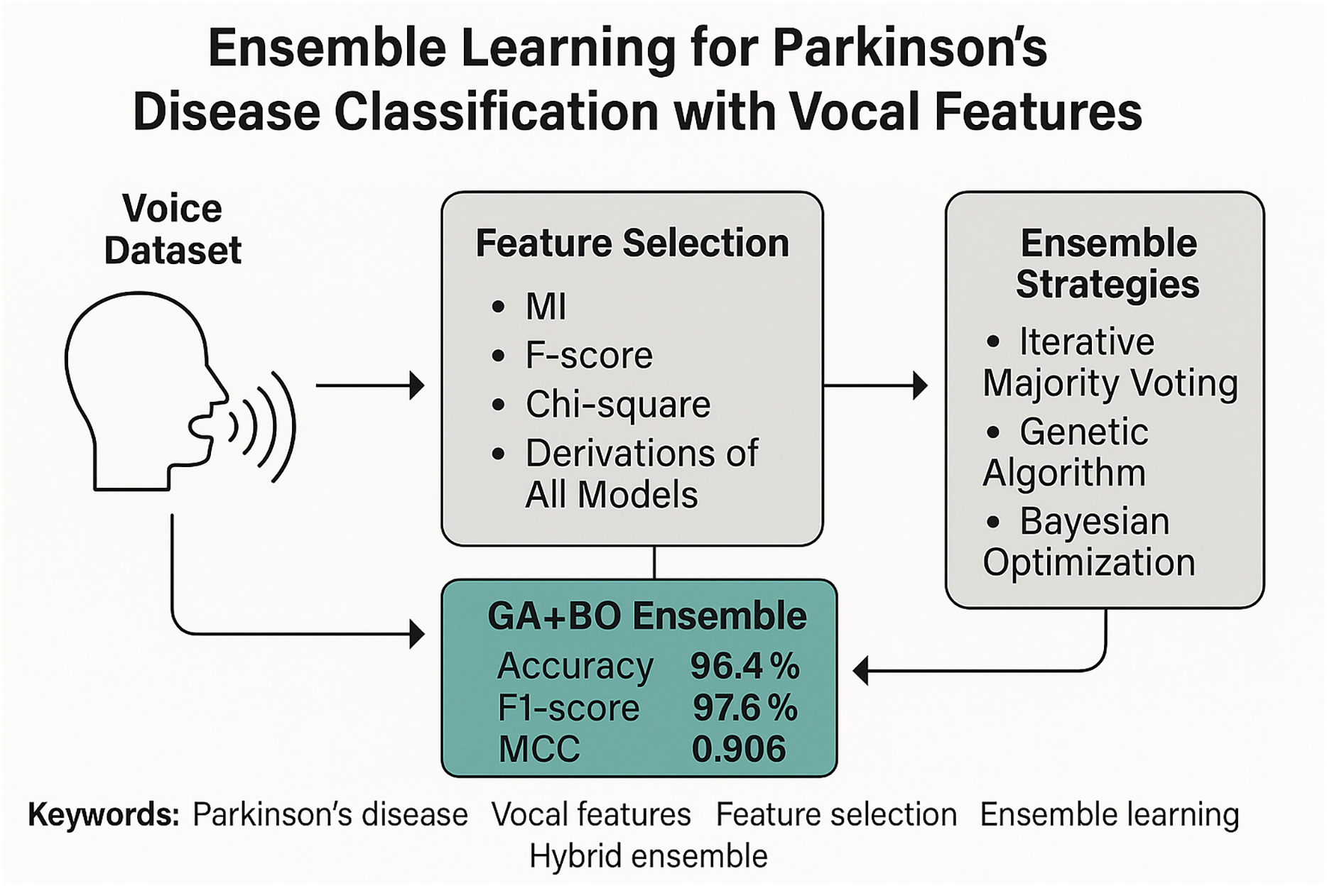
Figure 1 illustrates the overall architecture of the proposed framework through a graphical abstract. This high-level overview encapsulates the core stages of our methodology, beginning with raw vocal feature extraction and proceeding through multi-stage feature selection, classifier training, and ensemble integration. The pipeline highlights the use of three classical filter-based selection methods—Mutual Information (MI), F-score, and Chi-square—along with their composite derivations such as hybrid voting and score fusion. These selection techniques generate compact and informative feature subsets, which are then processed by multiple base classifiers. Finally, a hybrid ensemble strategy that combines GA for classifier selection and BO for adaptive weighting is employed to achieve robust PD classification. In the following subsections, we provide a detailed description of the dataset, feature sets, selection strategies, classifiers, and evaluation metrics that constitute this framework.

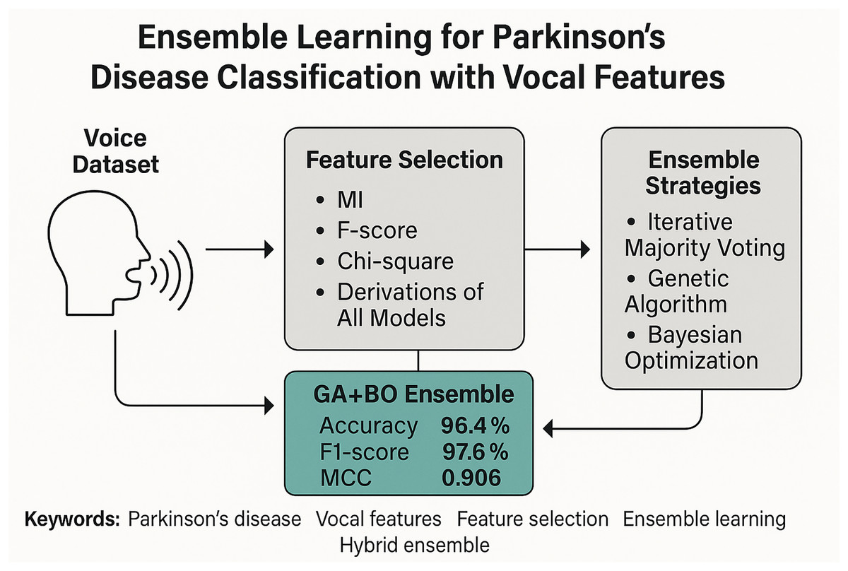
Figure 1: Graphical diagram of the proposed study.

Download full-size image

DOI: 10.7717/peerj-cs.3430/fig-1

Dataset

The dataset used in this study originates from the UCI Machine Learning Repository and was collected at the Department of Neurology, Cerrahpasa Faculty of Medicine, Istanbul University (Sakar et al., 2019). It comprises sustained phonation recordings of the vowel /a/ from 252 participants: 188 patients diagnosed with Parkinson’s disease (107 males, 81 females) and 64 healthy controls (23 males, 41 females). Subjects with PD ranged in age from 33 to 87 years, while healthy individuals were between 41 and 82 years. Each subject was asked to vocalize the sustained vowel three times, and recordings were captured at a sampling rate of 44.1 kHz.

The dataset includes a diverse array of vocal features extracted from time, frequency, and time-frequency domains. A total of 754 features were obtained and grouped into six primary categories, as summarized in Table 1.

Table 1:

Summary of feature sets and their dimensionality.

Feature set	Measure	# Features
Baseline features	Jitter variants	5
	Shimmer variants	6
	Fundamental frequency parameters	5
	Harmonicity parameters	5
	Recurrence Period Density Entropy (RPDE)	1
	Detrended Fluctuation Analysis (DFA)	1
	Pitch Period Entropy (PPE)	1
Time frequency features	Intensity parameters	3
	Formant frequencies	4
	Bandwidth	4
MFCCs	Mel frequency cepstral coefficients	84
Wavelet-based features	Wavelet transform features related with $F_{0}$	182
Vocal fold features	Glottis Quotient (GQ)	3
	Glottal to Noise Excitation (GNE)	6
	Vocal Fold Excitation Ratio (VFER)	7
	Empirical Mode Decomposition (EMD)	6
TQWT features	Tunable Q-factor Wavelet Transform features related with $F_{0}$	432

DOI: 10.7717/peerj-cs.3430/table-1

The key feature categories are described below:

Baseline features: This group includes traditional voice quality measures such as jitter, shimmer, harmonicity, and fundamental frequency statistics, along with nonlinear dynamic features (recurrence period density entropy (RPDE), detrended fluctuation analysis (DFA), pitch period entropy (PPE)) known to reflect neuromotor impairments in speech production.
MFCCs: A set of 84 Mel-Frequency Cepstral Coefficients—including log-energy, delta, and delta-delta coefficients—was extracted to capture articulatory behavior. MFCCs are particularly effective for modeling tongue and lip movements, which are often affected in PD.
Wavelet-based features (WT): A total of 182 features were derived from Discrete Wavelet Transform (DWT) applied to the F0 contour. These include signal energy, Shannon and log-energy entropies, and Teager–Kaiser energy extracted from both approximation and detail coefficients.
TQWT features: The Tunable Q-Factor Wavelet Transform (TQWT) was employed to model oscillatory impairments in voice by capturing fine-grained periodic disturbances in vocal fold vibrations. The dataset used in this study is publicly available and pre-processed, which facilitates consistent and reproducible feature extraction. Following prior evidence supporting the effectiveness of TQWT in biomedical vocal signal decomposition (Sakar et al., 2019), we adopted fixed parameter values of Q = 2, r = 4, and J = 35, resulting in the extraction of 432 features per instance.
Vocal fold and glottal features: This set includes GQ, GNE, VFER, and EMD-based measures, aiming to quantify glottal closure patterns, airflow turbulence, and phonatory noise—all of which are useful indicators of vocal fold dysfunction in PD.

To ensure a fair comparative analysis and mitigate potential bias arising from differences in feature set dimensionality, the experimental design was structured around three distinct groups of features:

Baseline + MFCC features: Combining classical acoustic markers and articulatory features for comprehensive phonation modeling.
Wavelet-based features (WT): Capturing multi-resolution frequency domain characteristics of the F0 signal.
TQWT features: Focused on detecting oscillatory degradation in voice with high frequency selectivity.

These subsets were evaluated separately to identify the most discriminative feature representations and to explore how different domains (time, frequency, and time frequency) contribute to the classification of PD. Prior to classification and feature selection, all features were normalized using min-max scaling to ensure consistent value ranges and eliminate potential scale-induced bias.

Feature selection methods

Feature selection is a critical preprocessing step in high-dimensional classification tasks, particularly for biomedical applications such as Parkinson’s disease diagnosis. In this study, we employ both traditional filter-based methods and several devised variants to reduce dimensionality, remove irrelevant features, and enhance classification performance.

Filter-based methods: Filter-based methods are computationally efficient and independent of any specific classifier. These methods evaluate each feature based on statistical criteria with respect to the target label, offering a scalable solution for large datasets (Theng & Bhoyar, 2024).

F-score: F-score evaluates the discriminative power of a feature by comparing inter-class and intra-class variances. For a feature $w_{j}$ , the F-score is defined as:

(1) $F (w_{j}) = \frac{{(μ^{+} - μ)}^{2} + {(μ^{-} - μ)}^{2}}{σ^{2 +} + σ^{2 -}}$ where $μ^{+}$ and $μ^{-}$ are the means of the feature for the positive and negative classes, $μ$ is the overall mean, and $σ^{2 +}$ , $σ^{2 -}$ are the variances within each class. A higher F-score indicates greater class separability (Yan et al., 2025).

Chi-square ( $χ^{2}$ ) Test: The $χ^{2}$ test assesses the dependency between features and class labels. For a feature $w_{j}$ and class $c_{i}$ , it is computed as:

(2) $χ^{2} (w_{j}, c_{i}) = \frac{N \cdot P_{j} (1, c_{i}) \cdot P_{j} (0, \bar{c_{i}}) - P_{j} (1, \bar{c_{i}}) \cdot P_{j} (0, c_{i})}{P_{j} (1) \cdot P_{j} (0) \cdot P (c_{i}) \cdot P (\bar{c_{i}})}$ where N is the total number of samples, and $P_{j}$ denotes the probabilities of feature-class co-occurrence and marginals (Abdo, Mostafa & Abdel-Hamid, 2024).

Mutual information (MI): Mutual information quantifies the amount of shared information between a feature $w_{j}$ and the class label C. It is defined as:

(3) $I (w_{j}; C) = \sum_{w \in {0, 1}} \sum_{c \in {- 1, 0, 1}} P_{j} (w, c) \log \frac{P_{j} (w, c)}{P_{j} (w) P (c)}$ This measure captures both linear and non-linear statistical dependencies, thereby offering robustness across heterogeneous and non-Gaussian data distributions (Gong et al., 2024). It is particularly well-suited for high-dimensional feature spaces where traditional correlation-based metrics may fail to identify informative patterns.

Devised feature selection variants: To further enhance the discriminative power of the selected features, we propose several hybrid and composite filter-based strategies that combine classical statistical metrics in systematically defined ways. These variants aim to exploit complementary strengths of $χ^{2}$ , MI, and F-score:

Hybrid voting: A majority-voting scheme is employed across the ranked lists of the three classical filters. Features appearing in the top- $k$ positions in at least two of the three rankings are retained. This method emphasizes consensus while tolerating mild divergence across ranking criteria.
Score fusion: Raw scores from $χ^{2}$ , MI, and F-score are min-max normalized to the $[0, 1]$ range to ensure comparability. The normalized scores are then aggregated via an unweighted arithmetic mean to compute a unified relevance score for each feature. Top- $k$ features with the highest composite scores are selected. This approach balances feature importance across heterogeneous criteria while preserving interpretability.
Intersect: Only features that concurrently appear in the top- $k$ lists of all three filter methods are selected. This conservative strategy emphasizes agreement and robustness, potentially favoring features with consistently high relevance across all criteria.
Union: All features that appear in at least one top- $k$ list are included. This inclusive approach maximizes feature diversity, potentially capturing complementary information, albeit at the cost of larger feature sets.
Classwise filtering: Each feature is evaluated separately for each class label (e.g., using class-conditional distributions in MI or F-score). The class-specific scores are then averaged to compute a balanced relevance score, mitigating class dominance and enhancing sensitivity to minority classes.

Each of these devised selection strategies is applied independently to Baseline + MFCC, Wavelet-based, and TQWT features thereby generating multiple reduced-dimensional representations for downstream ensemble learning and comparison.

Classifiers

Support vector machines

Support Vector Machines (SVM) are a commonly recognized supervised learning technique employed for both classification and regression problems. In the context of binary classification, SVM aims to pinpoint the best separating hyperplane by maximizing the distance, or margin, between data points of differing classes. In scenarios where the data cannot be linearly separated in the initial feature space, SVM leverages kernel functions to map the data into a higher-dimensional space, enabling linear separation. This mapping is accomplished using kernel methods like polynomial, radial basis function (RBF), or sigmoid kernels. The decision boundary is influenced by support vectors, which are the data points situated nearest to the separating hyperplane. A critical parameter in SVM models is the regularization constant C, which modulates the balance between maximizing the margin and reducing classification errors. A smaller C implies a broader margin with the possibility of misclassifying samples (underfitting), whereas a larger C aims to correctly classify every training instance, potentially causing overfitting (Rojas-Domínguez et al., 2017).

We used a polynomial kernel-based SVM classifier with degree set to three. Hyperparameters including C are tuned via a stratified 10-fold cross-validation scheme, ensuring robustness and generalizability of the trained models across all folds. This setup enables the classifier to effectively handle nonlinear patterns in vocal signal features associated with Parkinson’s disease.

k-nearest neighbors (KNN)

The $k$ -Nearest Neighbors algorithm is a widely adopted non-parametric classification method, particularly suitable for biomedical signal analysis, including voice-based PD (Nissar et al., 2019). The fundamental principle of KNN is to assign a class label to a test instance based on the majority class among its $k$ nearest neighbors in the feature space, where proximity is typically determined using the Euclidean distance metric.

Unlike parametric classifiers, $k$ -NN does not assume any prior distribution over the input data. Instead, it leverages the local geometry of the data manifold, making it well-suited for capturing intricate class boundaries when used in conjunction with appropriate feature representations and distance metrics.

In this study, we employ the $1$ -NN variant, wherein classification is determined solely by the single closest training instance. The selection of $k = 1$ is empirically motivated by preliminary stratified cross-validation experiments, which demonstrated that this configuration yields heightened sensitivity to subtle acoustic variations in the high-dimensional vocal features characteristic of Parkinsonian speech. Although computationally simple, $1$ -NN serves as a robust baseline within our ensemble learning framework, particularly when coupled with optimized feature subsets derived from the proposed selection methods.

All $k$ -NN models are evaluated using stratified 10-fold cross-validation to ensure statistical robustness and fair comparison across feature domains and classifiers (Zhang et al., 2017).

Majority voting-based ensemble methods

Given the diversity of features extracted from vocal signals, ensemble learning offers a promising strategy to consolidate the predictive power of individual models. Rather than relying on a single classifier trained on a specific feature subset, ensemble approaches aggregate outputs from multiple base learners, each trained on different representations. This not only enhances classification robustness but also mitigates model bias and variance. In this study, we propose and evaluate three distinct majority voting-based ensemble strategies tailored to exploit the complementary strengths of classifiers: Iterative Majority Voting (IMV), Genetic Algorithm-Based Voting (GA–Voting), and Bayesian Optimization-Based Voting (BO–Voting).

Iterative majority voting (IMV)

IMV begins with the best-performing individual classifier $h_{b e s t}$ and incrementally adds classifiers from the pool $H = {h_{1}, h_{2}, \dots, h_{K}}$ . At each step, the ensemble prediction ${\hat{y}}^{(t)}$ is computed using majority voting over selected classifiers $S^{(t)}$ :

(4) ${\hat{y}}^{(t)} = m o d e ({h_{i} (x) | h_{i} \in S^{(t)}})$

If the accuracy improves after adding $h_{j} \in H \ S^{(t)}$ , then $S^{(t + 1)} = S^{(t)} \cup {h_{j}}$ . This process continues until no further accuracy gain is observed (Tasci et al., 2024).

Genetic algorithm-based voting (GA–Voting)

GA–Voting frames the ensemble selection as a binary optimization problem. Each individual (chromosome) in the population is a binary vector $z \in {0, 1}^{K}$ indicating the inclusion of classifiers. The ensemble prediction is:

(5) ${\hat{y}}_{G A} = m o d e ({h_{i} (x) | z_{i} = 1}) .$

The fitness function $F (z)$ is defined as the validation accuracy of the ensemble formed by the selected classifiers:

(6) $F (z) = \frac{1}{N} \sum_{n = 1}^{N} I [{\hat{y}}_{G A}^{(n)} = y^{(n)}]$ where $I [\cdot]$ is the indicator function. Genetic operations such as crossover and mutation evolve the population toward higher fitness (Dhar, 2021).

Bayesian optimization-based voting (BO–Voting)

In BO–Voting, classifier outputs are weighted through soft voting. Each classifier $h_{i}$ is assigned a weight $w_{i} \in [0, 1]$ , forming a continuous weight vector $w \in [0, 1]^{K}$ under the constraint $Σ_{i = 1}^{K} w_{i} = 1$ . The aggregated score for class $c$ is:

(7) $s_{c} (x) = \sum_{i = 1}^{K} w_{i} \cdot I [h_{i} (x) = c] .$ The predicted class is then:

(8) ${\hat{y}}_{B O} = \arg max_{c} s_{c} (x) .$ BO is used to find the optimal $w^{*}$ that maximizes the ensemble accuracy:

(9) $w^{*} = \arg max_{w \in {[0, 1]}^{K}} \frac{1}{N} \sum_{n = 1}^{N} I [{\hat{y}}_{B O}^{(n)} = y^{(n)}] .$

This formulation enables adaptive weighting of classifiers, allowing stronger models to contribute more while suppressing weaker ones (Tasci, Uluturk & Ugur, 2021).

Together, these ensemble strategies allow a comparative investigation into how classifier selection (IMV, GA–Voting) and weighting (BO–Voting) impact diagnostic accuracy in PD classification. By integrating ensemble learning with diverse filter-based feature selection techniques, the proposed methods form a comprehensive framework for robust biomedical decision-making.

Evaluation method and metrics

To validate the effectiveness and generalizability of the proposed classifiers and ensemble strategies in distinguishing between PD patients and healthy controls, we adopt a stratified 10-fold cross-validation protocol as the primary evaluation method. In this approach, the dataset is divided into 10 mutually exclusive folds while preserving class distributions, and each fold is used once as a test set while the remaining nine folds are used for training. This process ensures robustness, reduces variance in performance estimation, and mitigates the risk of overfitting.

Following this procedure, we compute several standard performance metrics on each fold, including Accuracy, Precision, Recall, F-Measure, and the Matthews Correlation Coefficient (MCC). While accuracy is the most commonly reported indicator, it can be misleading under class imbalance. Therefore, we include additional metrics that provide a more balanced view of classifier performance.

Let the confusion matrix for binary classification be defined as:

True Positives (TP): correctly predicted PD cases,
False Positives (FP): healthy individuals misclassified as PD,
False Negatives (FN): PD patients misclassified as healthy,
True Negatives (TN): correctly predicted healthy individuals.

Based on these values, the evaluation metrics are calculated as follows:

(10) $A c c u r a c y = \frac{T P + T N}{T P + F P + F N + T N}$

(11) $P r e c i s i o n = \frac{T P}{T P + F P}$

(12) $R e c a l l = \frac{T P}{T P + F N}$

(13) $F 1 - s c o r e = 2 \times \frac{P r e c i s i o n \times R e c a l l}{P r e c i s i o n + R e c a l l} .$

Matthews Correlation Coefficient (MCC) is a robust metric that considers all four components of the confusion matrix. It yields a value between $- 1$ and $+ 1$ , where $+ 1$ indicates perfect classification, $0$ represents no better than random guessing, and $- 1$ indicates total disagreement:

(14) $M C C = \frac{(T P \times T N) - (F P \times F N)}{\sqrt{(T P + F P) (T P + F N) (T N + F P) (T N + F N)}} .$

These evaluation metrics, when computed over the repeated folds of the cross-validation procedure, provide a statistically reliable and comprehensive assessment of model performance. This ensures the proposed ensemble framework’s robustness and real-world applicability, even in the presence of imbalanced class distributions (Gunduz, 2021).

Experimental results

This section presents the experimental evaluation of the proposed PD classification framework using multiple vocal feature sets. Building upon the methods described in Methods Section, our approach integrates both filter-based feature selection techniques and hybrid ensemble strategies to improve classification performance.

As mentioned earlier, the dataset comprises three distinct groups of voice-based features derived from pathological speech recordings: (i) Wavelet Transform (WT) features ( $n = 182$ ), capturing localized frequency components from raw pitch contours; (ii) Baseline + MFCC features ( $n = 132$ ), which combine statistical acoustic descriptors with Mel-Frequency Cepstral Coefficients to model articulatory behavior; and (iii) Tunable Q-Factor Wavelet Transform (TQWT) features ( $n = 430$ ), designed to capture high-resolution oscillatory signal properties using tunable decomposition parameters. To identify the most informative and discriminative features from each group, we applied a total of eight feature selection strategies, comprising three traditional filter-based techniques—Chi-square, Mutual Information and F-score—as well as five ensemble-based selectors: hybrid, score fusion, union, intersect, and class-wise filtering. These methods were applied independently to each of the three feature groups, resulting in a total of 24 unique feature subsets (8 selectors $\times$ 3 feature groups).

Each selected feature subset was subsequently evaluated using two classifiers: KNN and SVM, both trained under a stratified 10-fold cross-validation protocol. This yielded a total of 48 distinct model configurations (24 feature subsets $\times$ 2 classifiers), whose outputs were recorded for further ensemble-based integration and comparative analysis. All experiments were conducted in the Google Colab environment, ensuring reproducibility and leveraging cloud-based computational resources for efficient execution.

To assess and highlight the most effective configurations, the performance of all individual models was ranked based on classification accuracy. The top 10 performing models were identified and listed in the results section, offering insights into the combinations of feature types, selection strategies, and classifiers that yielded the highest predictive accuracy for classification.

Baseline results without feature selection

To establish a performance baseline for our subsequent feature selection and ensemble learning strategies, we first evaluated the classification accuracy, F1-score, MCC, and average training time per fold using the entire set of features from each feature group—without applying any feature selection. These initial experiments were conducted using a 10-fold stratified cross-validation approach to ensure a balanced distribution of class labels across folds and to provide more reliable variance estimates.

We employed two classifiers: SVM using a polynomial kernel of degree 3, and KNN with $k = 1$ , across three primary feature groups. The results, reported as means and standard deviations across folds, are presented in Table 2, which includes the average running time per fold in seconds to reflect computational efficiency alongside predictive performance.

Table 2:

Baseline classification results using all features without selection (10-fold stratified CV).

Model	Accuracy	F1-score	MCC	Time (s)
Wavelet + KNN	$0.675 \pm 0.046$	$0.781 \pm 0.037$	$0.150 \pm 0.086$	$0.0032$
Wavelet + SVM	$0.747 \pm 0.019$	$0.853 \pm 0.012$	$0.100 \pm 0.116$	$0.0307$
TQWT + KNN	$0.903 \pm 0.030$	$0.936 \pm 0.019$	$0.741 \pm 0.086$	$0.0051$
TQWT + SVM	$0.861 \pm 0.032$	$0.913 \pm 0.019$	$0.607 \pm 0.102$	$0.0485$
Baseline_MFCC + KNN	$0.909 \pm 0.032$	$0.939 \pm 0.022$	$0.755 \pm 0.080$	$0.0027$
Baseline_MFCC + SVM	$0.847 \pm 0.032$	$0.901 \pm 0.020$	$0.570 \pm 0.096$	$0.0268$

DOI: 10.7717/peerj-cs.3430/table-2

These results indicate that, even without dimensionality reduction, both the Baseline_MFCC and TQWT feature sets achieved notably higher classification performance compared to the wavelet-based features. The KNN classifier consistently outperformed SVM in terms of accuracy, F1-score, and MCC across the two stronger feature sets. Additionally, KNN showed significantly lower average running time, reinforcing its suitability for real-time or resource-constrained settings.

These findings establish a strong reference point for evaluating the effectiveness and efficiency of the proposed feature selection and hybrid ensemble learning strategies presented in subsequent sections.

Performance with feature selection (Top 10 models)

To evaluate the impact of feature selection on classification performance, we applied multiple filter-based and hybrid methods using feature retention ratios of 20%, 40%, and 60%. The primary objective was to reduce the dimensionality of the original feature sets while preserving the most informative attributes. All models were trained using KNN and SVM classifiers across three major feature groups—TQWT, Baseline + MFCC, and Wavelet—using the selected subsets. As in the baseline evaluation, a 10-fold stratified cross-validation procedure was employed to ensure balanced representation of class labels in each fold and to obtain reliable variance estimates.

Table 3 presents the top 10 models at the 20% retention level, sorted by classification accuracy. Even with a reduced feature set, the TQWT-based models combined with KNN classifiers consistently achieved the highest performance. The best-performing model at this stage was TQWT + Hybrid + KNN, reaching an accuracy of $0.897 \pm 0.030$ , F1-score of $0.934 \pm 0.019$ , and MCC of $0.728 \pm 0.089$ with an average running time of 0.0023 s per fold. These results indicate that even when only 20% of the original features are retained, the classification performance remains competitive and, in many cases, surpasses the baseline models that utilize the complete feature sets.

Table 3:

Top 10 models with feature selection (feature ratio = 20%) based on classification accuracy (10-fold stratified CV).

Model	Accuracy	F1-score	MCC	Time (s)
TQWT + Hybrid + KNN	$0.897 \pm 0.030$	$0.934 \pm 0.019$	$0.728 \pm 0.089$	0.0023
TQWT + F-score + KNN	$0.890 \pm 0.046$	$0.926 \pm 0.030$	$0.710 \pm 0.132$	0.0024
TQWT + Chi² + KNN	$0.881 \pm 0.035$	$0.921 \pm 0.023$	$0.683 \pm 0.101$	0.0024
TQWT + Score fusion + KNN	$0.870 \pm 0.035$	$0.913 \pm 0.022$	$0.659 \pm 0.103$	0.0024
TQWT + MI + KNN	$0.861 \pm 0.041$	$0.907 \pm 0.027$	$0.634 \pm 0.110$	0.0024
TQWT + Intersect + KNN	$0.860 \pm 0.033$	$0.907 \pm 0.022$	$0.626 \pm 0.097$	0.0020
TQWT + Score fusion + SVM	$0.857 \pm 0.040$	$0.910 \pm 0.024$	$0.595 \pm 0.131$	0.0177
TQWT + Hybrid + SVM	$0.853 \pm 0.043$	$0.908 \pm 0.025$	$0.582 \pm 0.146$	0.0179
TQWT + Union + SVM	$0.853 \pm 0.045$	$0.908 \pm 0.027$	$0.582 \pm 0.147$	0.0172
TQWT + Chi² + SVM	$0.849 \pm 0.037$	$0.906 \pm 0.022$	$0.569 \pm 0.121$	0.0183

DOI: 10.7717/peerj-cs.3430/table-3

Table 4 shows the results for a 40% feature retention ratio. TQWT-based models continued to dominate, particularly when paired with KNN classifiers. Baseline + MFCC features combined with class-wise F-score or Chi-square selection also emerged as top performers, reflecting the benefits of class-dependent feature relevance scoring. The highest performance at this level was achieved by TQWT + Hybrid + KNN with an accuracy of $0.902 \pm 0.039$ , F1-score of $0.935 \pm 0.025$ , and MCC of $0.738 \pm 0.111$ .

Table 4:

Top 10 models with feature selection (feature ratio = 40%) based on classification accuracy (10-fold stratified CV).

Model	Accuracy	F1-score	MCC	Time (s)
TQWT + Hybrid + KNN	$0.902 \pm 0.039$	$0.935 \pm 0.025$	$0.738 \pm 0.111$	0.0044
TQWT + Intersect + KNN	$0.902 \pm 0.031$	$0.935 \pm 0.021$	$0.738 \pm 0.082$	0.0028
TQWT + F-score + KNN	$0.901 \pm 0.037$	$0.934 \pm 0.023$	$0.736 \pm 0.112$	0.0048
TQWT + MI + KNN	$0.899 \pm 0.020$	$0.932 \pm 0.013$	$0.727 \pm 0.061$	0.0049
Baseline_MFCC + F-score (Class-wise) + KNN	$0.897 \pm 0.031$	$0.932 \pm 0.021$	$0.721 \pm 0.083$	0.0021
Baseline_MFCC + Chi-square (Class-wise) + KNN	$0.897 \pm 0.031$	$0.932 \pm 0.021$	$0.721 \pm 0.083$	0.0020
TQWT + Union + KNN	$0.896 \pm 0.041$	$0.930 \pm 0.026$	$0.721 \pm 0.115$	0.0031
TQWT + Score fusion + KNN	$0.893 \pm 0.044$	$0.929 \pm 0.028$	$0.714 \pm 0.127$	0.0049
TQWT + Chi² + KNN	$0.892 \pm 0.040$	$0.928 \pm 0.025$	$0.709 \pm 0.117$	0.0047
TQWT + F-score (Class-wise) + KNN	$0.877 \pm 0.046$	$0.919 \pm 0.029$	$0.663 \pm 0.130$	0.0048

DOI: 10.7717/peerj-cs.3430/table-4

Finally, Table 5 reports results for a 60% feature retention ratio. TQWT-based models remained dominant, and class-specific feature selection methods further improved discriminative capacity. Notably, TQWT + F-score (Class-wise) + KNN and TQWT + Chi-square (Class-wise) + KNN both achieved the top performance with an accuracy of $0.933 \pm 0.025$ , F1-score of $0.955 \pm 0.016$ , and MCC of $0.819 \pm 0.069$ .

Table 5:

Top 10 models with feature selection (feature ratio = 60%) based on classification accuracy (10-fold stratified CV).

Model	Accuracy	F1-score	MCC	Time (s)
TQWT + F-score (Class-wise) + KNN	$0.933 \pm 0.025$	$0.955 \pm 0.016$	$0.819 \pm 0.069$	0.0036
TQWT + Chi-square (Class-wise) + KNN	$0.933 \pm 0.025$	$0.955 \pm 0.016$	$0.819 \pm 0.069$	0.0041
TQWT + Chi² + KNN	$0.919 \pm 0.020$	$0.946 \pm 0.013$	$0.784 \pm 0.055$	0.0036
TQWT + Hybrid + KNN	$0.910 \pm 0.018$	$0.941 \pm 0.011$	$0.761 \pm 0.057$	0.0036
Baseline_MFCC + F-score (Class-wise) + KNN	$0.910 \pm 0.036$	$0.940 \pm 0.023$	$0.760 \pm 0.099$	0.0037
Baseline_MFCC + Chi-square (Class-wise) + KNN	$0.910 \pm 0.036$	$0.940 \pm 0.023$	$0.760 \pm 0.099$	0.0036
TQWT + Union + KNN	$0.909 \pm 0.021$	$0.940 \pm 0.013$	$0.754 \pm 0.066$	0.0037
TQWT + F-score + KNN	$0.907 \pm 0.020$	$0.939 \pm 0.012$	$0.750 \pm 0.064$	0.0038
TQWT + Intersect + KNN	$0.903 \pm 0.042$	$0.936 \pm 0.028$	$0.748 \pm 0.114$	0.0030
Baseline_MFCC + MI + KNN	$0.896 \pm 0.020$	$0.930 \pm 0.013$	$0.724 \pm 0.056$	0.0035

DOI: 10.7717/peerj-cs.3430/table-5

These findings confirm that even under reduced or fixed feature budgets, TQWT-based features combined with KNN classifiers consistently achieve superior performance. Class-dependent feature selection methods further enhance discriminative capacity, especially at larger feature retention ratios, while maintaining low average running times per fold.

To ensure a fair and controlled comparison among the three feature groups—TQWT, Baseline + MFCC, and Wavelet—we fixed the number of selected features to 100 per group. This constraint allows observed performance differences to be attributed solely to the discriminative capacity of each feature type, eliminating the potential confounding effect of varying feature dimensionality. Using the same set of filter-based selection methods, both KNN and SVM classifiers were evaluated on each feature group. The results are summarized in Table 6. Among all evaluated models, the best performance was achieved by the configuration using Baseline + MFCC features with Score Fusion and KNN classifier, yielding an accuracy of $0.905 \pm 0.027$ , F1-score of $0.936 \pm 0.019$ , and MCC of $0.750 \pm 0.069$ . Overall, MFCC-based KNN models consistently outperformed their TQWT and Wavelet counterparts when constrained to a uniform feature count. Moreover, KNN demonstrated superior performance compared to SVM across all feature sets, highlighting its robustness in low-dimensional settings.

Table 6:

Top-performing models with fixed 100-feature subset per feature group (10-fold stratified CV).

Time indicates average runtime per fold.

Model	Accuracy	F1-score	MCC	Time (s)
Baseline MFCC + Score fusion + KNN	$0.905 \pm 0.027$	$0.936 \pm 0.019$	$0.750 \pm 0.069$	0.0025
Baseline_MFCC + MI + KNN	$0.903 \pm 0.017$	$0.935 \pm 0.012$	$0.747 \pm 0.044$	0.0025
Baseline_MFCC + F-score (Class-wise) + KNN	$0.902 \pm 0.027$	$0.935 \pm 0.019$	$0.736 \pm 0.068$	0.0025
Baseline_MFCC + Chi-square (Class-wise) + KNN	$0.899 \pm 0.027$	$0.933 \pm 0.019$	$0.736 \pm 0.068$	0.0026
Baseline_MFCC + Hybrid + KNN	$0.894 \pm 0.025$	$0.929 \pm 0.017$	$0.720 \pm 0.068$	0.0024
Baseline_MFCC + Chi² + KNN	$0.889 \pm 0.034$	$0.925 \pm 0.023$	$0.708 \pm 0.091$	0.0024
Baseline_MFCC + MI (Class-wise) + KNN	$0.889 \pm 0.046$	$0.926 \pm 0.031$	$0.701 \pm 0.125$	0.0024
Baseline_MFCC + F-score + KNN	$0.888 \pm 0.022$	$0.925 \pm 0.015$	$0.701 \pm 0.058$	0.0025
Baseline_MFCC + Union + KNN	$0.888 \pm 0.022$	$0.925 \pm 0.015$	$0.701 \pm 0.058$	0.0033
Baseline_MFCC + Intersect + KNN	$0.885 \pm 0.033$	$0.922 \pm 0.024$	$0.700 \pm 0.073$	0.0024

DOI: 10.7717/peerj-cs.3430/table-6

These results confirm that, even under a uniform feature selection budget, Baseline + MFCC features combined with ensemble-based selection strategies such as Score Fusion and class-wise statistical filters offer the highest discriminative capacity for PD classification.

To assess the impact of different feature retention levels on classification performance, we conducted an evaluation using 20%, 40%, 60% of the ranked features as well as a fixed selection of the top 100 features. The box plot in Fig. 2 visualizes the accuracy distribution across multiple runs.

Figure 2: Box plot comparison of classification accuracies at different feature retention levels (20%, 40%, 60%, and 100 features).
The 60% retention consistently yielded better median accuracy and lower variance, motivating its selection for ensemble modeling.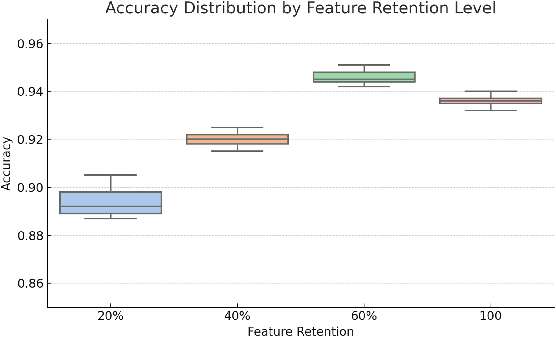

Download full-size image

DOI: 10.7717/peerj-cs.3430/fig-2

As seen in the plot, 60% feature retention yielded the highest median accuracy and a tighter interquartile range, suggesting improved generalizability. These findings guided our decision to use the 60% threshold for subsequent ensemble construction.

Ensemble learning strategies and hybrid integration

To further enhance classification performance while maintaining fairness across feature groups, we explored a set of ensemble learning strategies applied to models trained with the top-performing 60% feature retention from each group. These strategies aim to leverage the complementary strengths of individual classifiers through systematic combination and optimization.

Three principal ensemble methods were investigated:

Iterative Majority Voting (IMV): A sequential ensemble construction approach that incrementally adds high-performing base models. At each step, the ensemble output is determined via majority voting, and the configuration yielding the highest classification accuracy is retained.
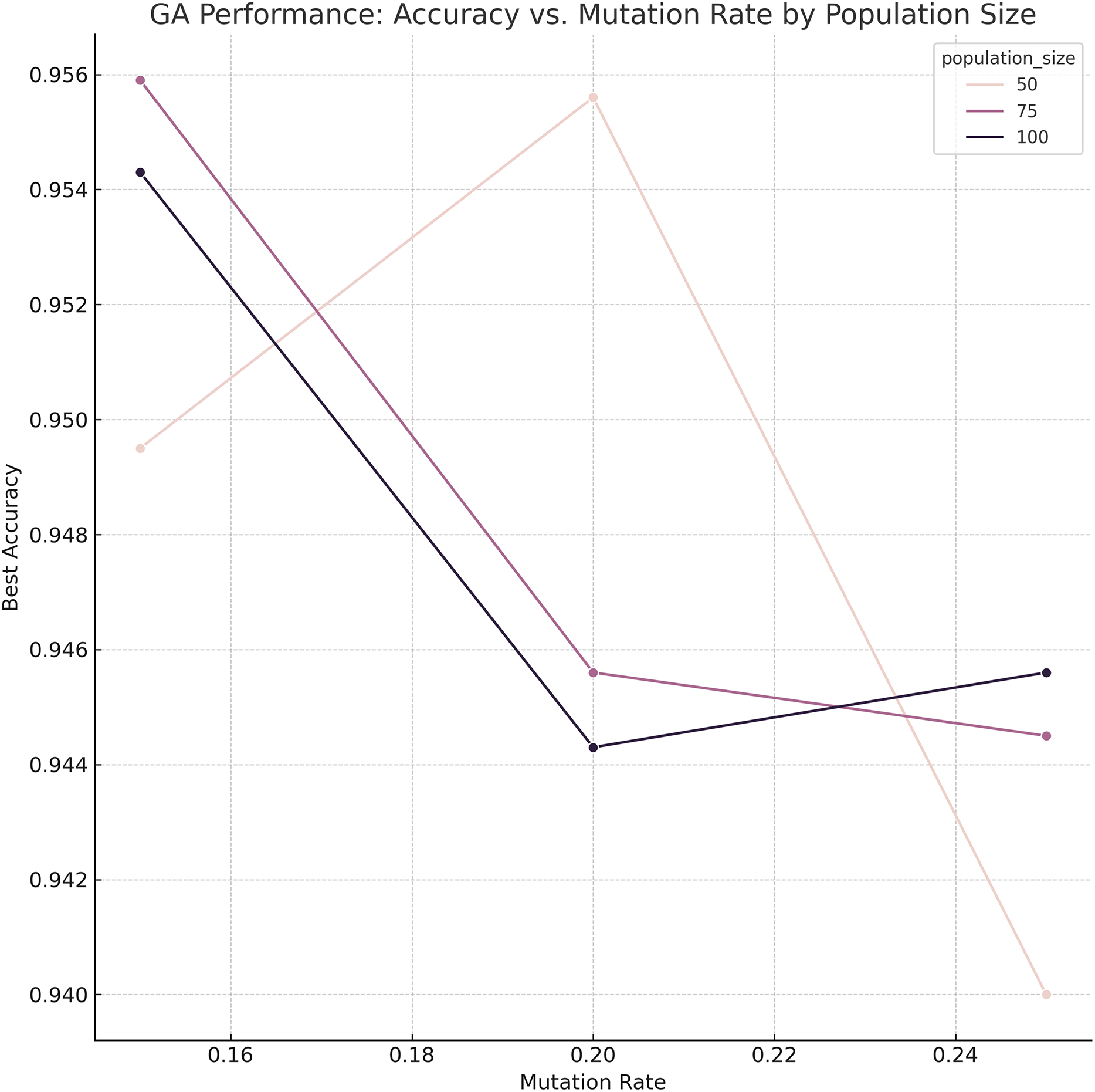
Genetic Algorithm-based Ensemble (GA–Ensemble): This method formulates model selection as an optimization problem and uses a genetic algorithm to identify the most effective subset of base classifiers. The GA was initially configured with a population size of 75, 150 generations, a mutation rate of 0.15, and tournament selection for parent selection. To ensure that these hyperparameters were not arbitrarily chosen, a grid search was conducted over multiple candidate configurations (population size, mutation rate, and number of generations). The results of this search and the sensitivity of GA to these parameters are visualized in Fig. 3. The figure reveals that higher population sizes and lower mutation rates tend to improve ensemble performance by enhancing exploration without sacrificing convergence stability.
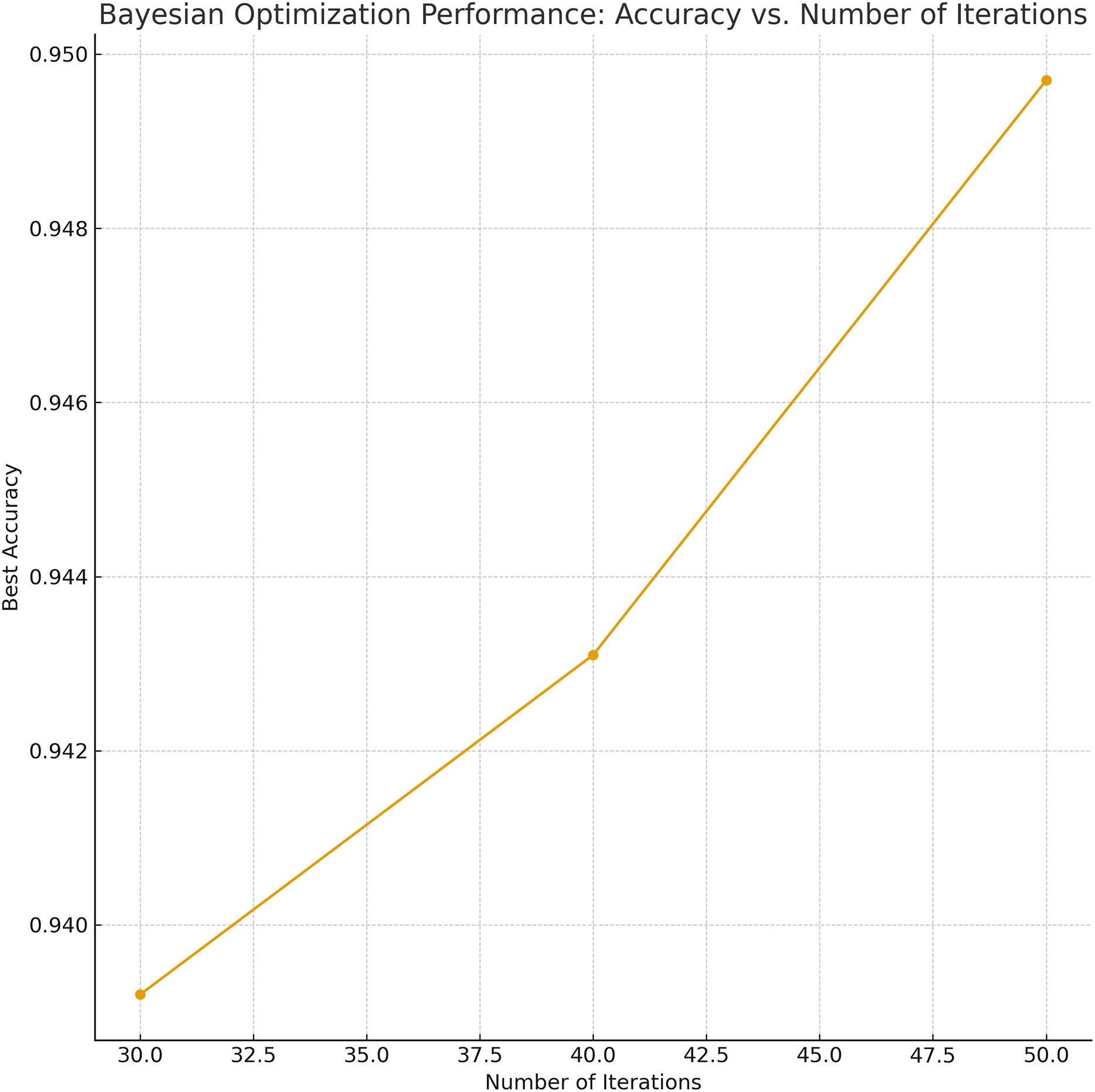
Bayesian Optimization-based Weighted Ensemble (BO–Ensemble): This strategy employs probabilistic modeling to assign dynamic weights to base models, enabling a soft-voting mechanism. The BO procedure began with 10 initial random samples and was iterated 50 times to find the optimal weight configuration. Similar to GA, the number of iterations and initial sample sizes for BO were also selected via grid search, and the parameter sensitivity is depicted in Fig. 4. The analysis indicates that 30–50 iterations strike a balance between performance gain and computational cost, stabilizing weight tuning across diverse base classifiers.

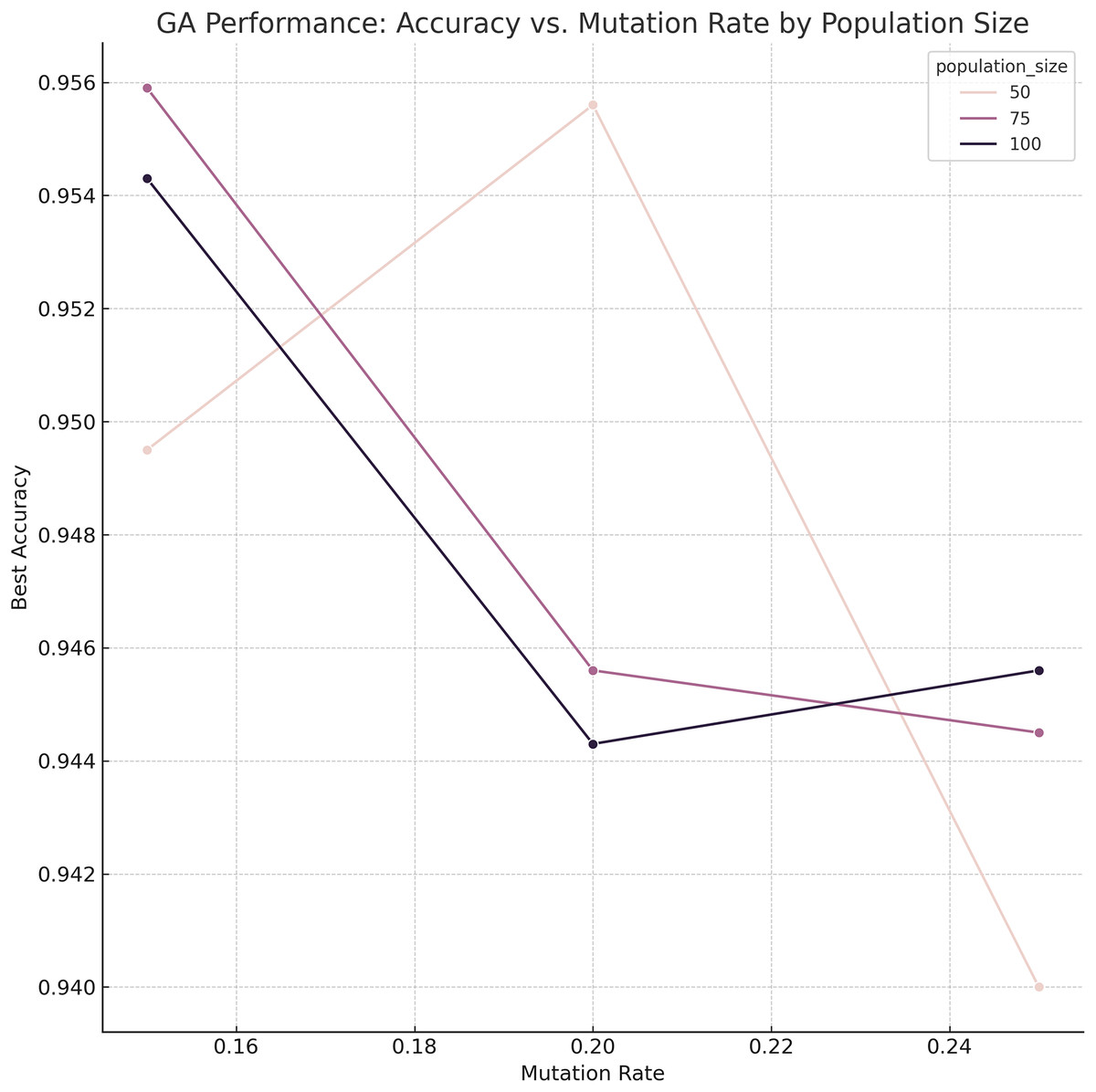
Figure 3: Sensitivity analysis and grid-search results for GA parameters (population size, mutation rate).

Download full-size image

DOI: 10.7717/peerj-cs.3430/fig-3

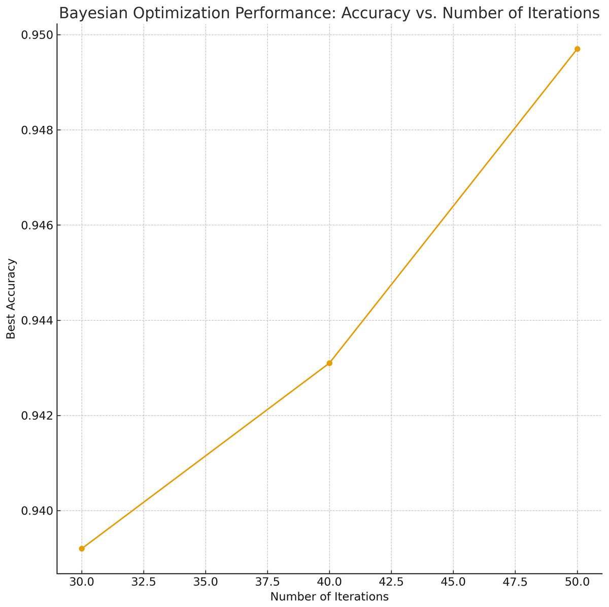
Figure 4: Sensitivity analysis and grid-search results for BO parameters (number of iterations).

Download full-size image

DOI: 10.7717/peerj-cs.3430/fig-4

Building on these approaches, we propose a novel two-stage hybrid model, denoted as GA–BO–Ensemble, which first applies GA to determine a high-quality subset of base models and subsequently uses BO to fine-tune the fusion weights. This hybrid strategy combines the benefits of selective inclusion and adaptive weighting, offering improved robustness and predictive accuracy.

Algorithm 1 outlines the proposed GA–BO–Ensemble integration process, which proceeds in three systematic stages. In the first stage, a population of binary chromosomes is initialized, where each chromosome encodes a subset of base classifiers. The GA evolves this population over multiple generations using a fitness function based on majority voting accuracy. Through selection, crossover, and mutation operations, the algorithm converges on an optimal subset of models that exhibit high discriminative performance. In the second stage, BO is employed to determine the optimal soft-voting weights for the selected models. This is achieved by maximizing ensemble accuracy via adaptive tuning of real-valued weights under a unit-sum constraint. In the final stage, class predictions are generated by computing a weighted sum of the selected model outputs, and the label with the highest aggregated score is assigned. This two-tiered strategy ensures both selective inclusion of competent models and dynamic weighting based on individual reliability, yielding a robust and accurate ensemble framework.

Algorithm 1 :

Hybrid GA–BO ensemble integration algorithm.

Input:

P = {P_{1}, P_{2}, \dots, P_{K}}

: Classifier predictions

Y: True class labels

G: Number of generations

M: Population size

r: Mutation rate

Output:

S^{*}

: Selected classifier subset

w^{*}

: Optimized weights

\hat{Y}

: Final predictions

Step 1: Genetic Algorithm for Subset Selection

Initialize a population

Z = {z_{1}, z_{2}, \dots, z_{M}}

where

z_{i} \in {0, 1}^{K}

for each generation

g = 1

to G do

Evaluate fitness of each z_i as classification accuracy using majority voting over selected P_k

Select elite z_e with highest fitness and add to next population

While new population

< M

Select two parents and perform one-point crossover

Apply bit-flip mutation to offspring with rate r

Add offspring to new population

Replace old population with new population

Select

S^{*}

from best-performing chromosome

z^{*}

Step 2: Bayesian Optimization for Weight Learning

One-hot encode Y and prediction vectors in

S^{*}

Define soft voting function using weights

w

Use Bayesian Optimization to maximize voting accuracy over

w

Return optimal weights

w^{*}

Step 3: Final Ensemble Prediction

Compute weighted sum of predictions using

w^{*}

Assign class labels by argmax over weighted scores:

\hat{Y} = \arg max_{c} Σ w_{k} P_{k}

return

S^{*}

w^{*}

\hat{Y}

DOI: 10.7717/peerj-cs.3430/table-101

To evaluate the effectiveness of the proposed GA–BO hybrid ensemble, we conducted an ablation study comparing its performance against three ensemble variants: GA-only, BO-only and IMV. The results are presented in Table 7.

Table 7:

Comparison of ensemble strategies on Parkinson’s Disease classification (mean

\pm

std).

Wilcoxon test conducted against GA–BO–Ensemble.

Ensemble strategy	Accuracy	F1-score	MCC	Wilcoxon $p$ -value	Time (s)
Iterative Majority Voting (IMV)	0.9525 $\pm$ 0.0236	0.9691 $\pm$ 0.0149	0.8722 $\pm$ 0.0659	0.2969	20.53
Genetic Algorithm (GA)	0.9444 $\pm$ 0.0175	0.9639 $\pm$ 0.0111	0.8507 $\pm$ 0.0492	0.0039	34.21
Bayesian Optimization (BO)	0.9537 $\pm$ 0.0179	0.9699 $\pm$ 0.0113	0.8759 $\pm$ 0.0506	0.0625	203.88
GA–BO–Ensemble	$0.9643 \pm 0.0196$	$0.9764 \pm 0.0128$	$0.9047 \pm 0.0539$	1.0000	103.12

DOI: 10.7717/peerj-cs.3430/table-7

The GA–BO hybrid ensemble achieved the best overall performance across all metrics, with an accuracy of 0.9643, F1-score of 0.9764, and MCC of 0.9047. Statistical analysis using the Wilcoxon signed-rank test confirmed the superiority of GA–BO over GA-only ( $p$ = 0.0039), with no significant difference observed when compared to BO-only or IMV ( $p > 0.05$ ). In terms of execution time, GA–BO (103.12 s) balances between the fast but less adaptive GA (34.21 s) and the computationally expensive BO-only approach (203.88 s).

These results highlight the synergistic advantages of the two-stage GA–BO integration. The GA module performs a structural selection by pruning suboptimal or redundant base classifiers, thereby enhancing ensemble diversity and reducing overfitting risk. The BO component subsequently assigns optimized probabilistic weights to the remaining classifiers, capturing fine-grained inter-model dependencies. In contrast, the GA-only method lacks the flexibility to tune the relative importance of selected models, while the BO-only approach may overfit due to assigning weights across a larger, unfiltered classifier pool. By combining structural pruning with adaptive weighting, the GA–BO hybrid strategy offers a principled and computationally balanced approach to ensemble construction. This yields improved robustness and discriminative capacity in classification.

Conclusion and discussion

This study presents a comprehensive and computationally efficient framework for PD classification using vocal features. Our results demonstrate that high classification accuracy can be achieved through selective feature optimization and lightweight ensemble learning strategies—without relying on deep or computationally intensive architectures.

A central contribution of this work is the systematic evaluation of three prominent feature groups—TQWT, Baseline + MFCC, and conventional Wavelet features—across eight feature selection techniques. Among these, the TQWT-based features consistently yielded superior performance, especially when combined with class-wise filter-based selectors and the KNN classifier. The best-performing filter-based configuration, which integrated TQWT features with class-wise F-score selection and KNN, achieved an accuracy of 93.3% and an F1-score of 95.5%, outperforming many existing approaches in the literature.

A notable observation is the shift in performance rankings between the percentage-based feature retention settings (Tables 3–5) and the fixed-size feature evaluation (Table 6). In the percentage-based evaluations, TQWT features consistently outperformed Baseline + MFCC and Wavelet features across most metrics. This suggests that the discriminative information in TQWT features is more diffusely distributed, requiring a larger proportion of features to retain class-separability. In contrast, the fixed-size (100-feature) analysis revealed that Baseline + MFCC features yielded the best performance, indicating that MFCC-based representations concentrate more relevant information in a smaller subset of dimensions. These findings highlight important implications for real-time systems: TQWT-based models benefit from higher feature budgets, while MFCCs are preferable for compact, low-latency models.

Another strength of the proposed framework is its ensemble-based feature selection strategy. Instead of relying on a single filter method, hybrid and consensus-based techniques, such as score fusion, union, and intersection, were employed to harness complementary strengths. This multi-strategy approach enhanced both the discriminative power and stability of selected features across validation folds, echoing recent findings in the literature that advocate multi-level dimensionality reduction pipelines. The integration of a two-stage ensemble strategy (GA–BO Ensemble) further enhanced performance. This hybrid ensemble method achieved the highest overall accuracy (96.43%), F1-score (97.64%), and MCC (0.9047) across all experiments, establishing it as the most robust and discriminative model in the study. Its success is attributed to the synergy between GA’s structural pruning and BO’s probabilistic weight tuning, effectively combining model diversity and optimal voting dynamics. Table 8 compares our approach with recent studies that employed acoustic features for PD detection.

Table 8:

Comparison of recent methods for PD detection using acoustic features.

Author(s)	Methodology	Accuracy (%)
Gunduz (2019)	CNN (no FS)	86.90
Quan, Ren & Luo (2021)	Bi-LSTM (no FS)	84.29
Pramanik et al. (2021)	DF (no FS)	94.12
Gunduz (2021)	Multi-Kernel SVM + Relief + Fisher score (30 features)	91.60
Lamba, Gulati & Jain (2022)	MIRFE + XGBoost	93.88
Ouhmida et al. (2024)	DNN + HEFS-MLDR (ReliefF + mRMR + Chi²)	97.08
Our study	KNN + Filter selection + GA–BO–Ensemble (453 features)	96.40

DOI: 10.7717/peerj-cs.3430/table-8

Compared to deep learning-based models such as CNNs (Gunduz, 2019) and DNNs (Ouhmida et al., 2024), our framework offers a superior balance between accuracy and computational cost. Deep models typically require extensive annotated datasets, high-performance GPUs, and long training times, which hinder deployment in low-resource or real-time clinical settings. In contrast, our hybrid ensemble approach achieves comparable accuracy without the heavy computational burden, making it suitable for edge devices and mobile health platforms.

Table 9 highlights the efficiency of the GA–BO–Ensemble model by comparing its cross-validation runtime with two deep learning baselines. The GA–BO model completed all folds in 103.12 s—significantly faster than the 771.21 s required by Gunduz (2019), despite the latter using GPU-based training. It also outperformed the HEFS-MLDR model by Ouhmida et al. (2024), which completed in 137.58 s.

Table 9:

Comparison of training and inference times with SOTA deep learning models.

Model	Accuracy ( $\pm$ std)	F1-score ( $\pm$ std)	MCC ( $\pm$ std)	CV Time (s)
GA–BO–Ensemble (ours)	0.9643 $\pm$ 0.0196	0.9764 $\pm$ 0.0128	0.9047 $\pm$ 0.0539	103.12
Ouhmida et al. (2024)	0.9100 $\pm$ 0.0347	0.9417 $\pm$ 0.0221	0.7565 $\pm$ 0.1009	137.58
Gunduz (2019)	0.8609 $\pm$ 0.0566	0.9083 $\pm$ 0.0339	0.6096 $\pm$ 0.2296	771.21*

DOI: 10.7717/peerj-cs.3430/table-9

Note:

* Utilized GPU-based training.

Limitations

Despite the demonstrated effectiveness of the proposed GA–BO-based ensemble framework, several limitations warrant consideration.

First, the sequential nature of the GA followed by BO introduces potential biases related to the convergence path. Since GA serves as an initial heuristic search and BO subsequently refines the solution space, early suboptimal feature subsets identified by GA may constrain BO’s exploration capacity, potentially resulting in local optima. Future work could address this by integrating hybrid feedback mechanisms or employing multi-objective search strategies to improve convergence robustness.

Second, the reliance on the 1-NN classifier in several experiments, while interpretable and effective for clean datasets, presents challenges in noisy or high-dimensional feature spaces. Its sensitivity to local outliers and vulnerability to the curse of dimensionality could impair generalization performance on real-world, less curated clinical data. This motivates further benchmarking with more noise-robust classifiers (e.g., ensemble-based or probabilistic models) to strengthen performance under adverse conditions.

Third, although the proposed pipeline achieves competitive accuracy, its multi-stage design inherently increases training-time computational cost due to repeated evaluations across meta-heuristic iterations. This may limit scalability to larger datasets or real-time applications unless optimized further through parallelization or early stopping strategies.

Finally, a key limitation of this study lies in its evaluation on a single benchmark dataset. While the dataset is publicly available and widely used, the absence of cross-corpus validation restricts the assessment of the model’s robustness across different recording setups, accents, and demographics. Addressing this gap will be a key priority in future work through cross-dataset validation and adaptation studies.

Nevertheless, these limitations also underscore the need to examine the algorithmic complexity and scalability of the proposed framework—a pathway toward practical deployment and clinical integration, as elaborated in the following sections.

Algorithmic complexity

The proposed framework comprises three sequential computational stages during training—(i) filter-based feature selection, (ii) GA for ensemble subset selection, and (iii) BO for weight tuning. While these stages incur moderate training overhead, the inference pipeline remains lightweight and scalable, ensuring real-time applicability in clinical environments. Below, we summarize the theoretical time complexities of each component:

Filter-based feature selection: For $n$ samples and $d$ features, classical univariate filters (e.g., $χ^{2}$ , F-score, Mutual Information) require $O (n \cdot d)$ operations, as each feature is evaluated independently. These methods are non-iterative and parallelizable.
GA-based ensemble subset selection: Let P be the population size, G the number of generations, and $T_{e v a l}$ the cost of evaluating a single solution (e.g., via $k$ -fold cross-validation). The total complexity is $O (P \cdot G \cdot T_{e v a l})$ , where $T_{e v a l} = O (k \cdot n)$ . Given bounded P and G, the cost remains tractable.
BO-based weight optimization: For $b$ iterations in a C-dimensional continuous search space (where C is the number of classifiers), BO using Gaussian Process regression incurs $O (b \cdot C^{2})$ complexity due to kernel matrix inversion. In our setting, both $b$ and C are small (e.g., $b \leq 50$ , $C \leq 24$ ), resulting in efficient convergence.
Inference phase: Given $k$ selected classifiers and $m$ features per instance, the prediction phase requires $O (k \cdot m)$ operations. This minimal cost supports deployment on edge devices and integration in time-sensitive clinical workflows.

Overall, the full training complexity is bounded by:

$O (n \cdot d + P \cdot G \cdot k \cdot n + b \cdot C^{2})$ whereas inference remains constant-time with respect to data size. Since training is performed offline and each component is amenable to parallelization, the framework ensures a favorable trade-off between training efficiency and runtime deployment scalability.

Clinical translation and deployment

While the proposed GA–BO-powered framework demonstrates strong performance in experimental settings, transitioning this system into a clinically viable decision support tool necessitates several concrete steps. Given that the model relies solely on speech data, it presents a non-invasive, accessible, and low-cost modality for the early detection and monitoring of PD. This enables integration into diverse deployment environments, including smartphone-based mobile applications, telemedicine platforms, and outpatient clinic interfaces for routine screening. Such a system could assist neurologists in identifying at-risk individuals, particularly in underserved regions lacking access to movement disorder specialists, and could also serve as a supplementary tool for longitudinal disease tracking.

To facilitate clinical translation, future efforts will focus on:

testing the model on larger and more demographically diverse patient cohorts across multiple datasets to evaluate generalizability,
conducting prospective clinical studies in collaboration with neurology departments to validate real-world performance,
enhancing model transparency and interpretability through post hoc techniques such as SHAP or LIME, and
integrating the system into existing electronic health record (EHR) workflows to support seamless adoption by healthcare providers.

These steps will help transition the current research prototype into a robust, scalable, and clinically deployable decision support system for PD diagnosis and ongoing patient monitoring.

Future work

Beyond the clinical translation goals discussed in the previous subsection, several directions remain open for further research and methodological refinement. First, the current sequential design of the GA–BO ensemble introduces potential convergence bias, where suboptimal solutions from the GA may constrain the effectiveness of the subsequent Bayesian optimization phase. Future work will explore hybrid or co-evolutionary optimization strategies to mitigate such biases and improve global search capacity.

Second, while the 1-NN classifier was chosen for its interpretability, it may be susceptible to noise in more heterogeneous or high-dimensional clinical datasets. Subsequent studies will evaluate alternative classifiers, including ensemble-based and probabilistic models, for improved robustness.

Third, although the current framework achieves competitive performance, the training pipeline is computationally intensive due to meta-heuristic iterations. Future work will involve streamlining the training process through surrogate-assisted evaluation, parallelization, or adaptive resource allocation strategies to enable scalability for larger cohorts.

Finally, to assess generalizability, planned studies will extend the evaluation to additional benchmark datasets with diverse recording protocols and demographics. These investigations will also include transfer learning and domain adaptation methods to bridge dataset-specific variations and support broader clinical deployment.

Supplemental Information

README file: Introduce and explain the code; provide steps for implementation.

DOI: 10.7717/peerj-cs.3430/supp-1

Download

[1] Abdel-fattah MA, Eid RH, Yakoub AE. 2023. A hybrid approach for enhancing the classification of the Parkinson’s disease using swarm optimization. Journal of Theoretical and Applied Information Technology 101(9)

[2] Abdo A, Mostafa R, Abdel-Hamid L. 2024. An optimized hybrid approach for feature selection based on chi-square and particle swarm optimization algorithms. Data 9(2):20

[3] Akila B, Nayahi JJV. 2024. Parkinson classification neural network with mass algorithm for processing speech signals. Neural Computing and Applications 36(17):10165-10181

[4] Bdaqli M, Shoeibi A, Moridian P, Sadeghi D, Pouyani MF, Shalbaf A, Gorriz JM. 2024. Diagnosis of Parkinson disease from EEG signals using a CNN-LSTM model and explainable AI. In: International Work-Conference on the Interplay Between Natural and Artificial Computationn. Cham: Springer Nature Switzerland. 123-138

[5] Cai Z, Gu J, Chen H-L. 2017. A new hybrid intelligent framework for predicting Parkinson’s disease. IEEE Access 5:17188-17200

[6] Cai Z, Gu J, Wen C, Zhao D, Huang C, Huang H, Tong C, Li J, Chen H. 2018. An intelligent Parkinson’s disease diagnostic system based on a chaotic bacterial foraging optimization enhanced fuzzy KNN approach. Computational and Mathematical Methods in Medicine 2018(1):2396952

[7] Chen H-L, Huang C-C, Yu X-G, Xu X, Sun X, Wang G, Wang S-J. 2013. An efficient diagnosis system for detection of Parkinson’s disease using fuzzy k-nearest neighbor approach. Expert Systems with Applications 40(1):263-271

[8] Chen H-L, Wang G, Ma C, Cai Z-N, Liu W-B, Wang S-J. 2016. An efficient hybrid kernel extreme learning machine approach for early diagnosis of Parkinson’s disease. Neurocomputing 184(6):131-144

[9] Dao SV, Yu Z, Tran LV, Phan PN, Huynh TT, Le TM. 2022. An analysis of vocal features for Parkinson’s disease classification using evolutionary algorithms. Diagnostics 12(8):1980

[10] Dhar J. 2021. Multistage ensemble learning model with weighted voting and genetic algorithm optimization strategy for detecting chronic obstructive pulmonary disease. IEEE Access 9:48640-48657

[11] Diaz M, Ferrer MA, Impedovo D, Pirlo G, Vessio G. 2019. Dynamically enhanced static handwriting representation for Parkinson’s disease detection. Pattern Recognition Letters 128(5):204-210

[12] Elkharadly M, Amin K, Abo-Seida O, Ibrahim M. 2025. Bayesian optimization enhanced FKNN model for Parkinson’s diagnosis. Biomedical Signal Processing and Control 100:107142

[13] El Maachi I, Bilodeau G-A, Bouachir W. 2020. Deep 1D-ConvNet for accurate Parkinson disease detection and severity prediction from gait. Expert Systems with Applications 143:113075

[14] Goberman AM, Blomgren M, Metzger E. 2010. Characteristics of speech disfluency in Parkinson disease. Journal of Neurolinguistics 23(5):470-478

[15] Goldman JG, Vernaleo BA, Camicioli R, Dahodwala N, Dobkin RD, Ellis T, Galvin JE, Marras C, Edwards J, Fields J, Golden R, Karlawish J, Levin B, Shulman L, Smith G, Tangney C, Thomas CA, Tröster AI, Uc EY, Coyan N, Ellman C, Ellman M, Hoffman C, Hoffman S, Simmonds D. 2018. Cognitive impairment in Parkinson’s disease: a report from a multidisciplinary symposium on unmet needs and future directions to maintain cognitive health. npj Parkinson’s Disease 4:19

[16] Gong H, Li Y, Zhang J, Zhang B, Wang X. 2024. A new filter feature selection algorithm for classification task by ensembling pearson correlation coefficient and mutual information. Engineering Applications of Artificial Intelligence 131(22):107865

[17] Gunduz H. 2019. Deep learning-based Parkinson’s disease classification using vocal feature sets. IEEE Access 7:115540–115551

[18] Gunduz H. 2021. An efficient dimensionality reduction method using filter-based feature selection and variational autoencoders on Parkinson’s disease classification. Biomedical Signal Processing and Control 66(4–5):102452

[19] Islam MA, Majumder MZH, Hussein MA, Hossain KM, Miah MS. 2024. A review of machine learning and deep learning algorithms for Parkinson’s disease detection using handwriting and voice datasets. Heliyon 10(3):e25469

[20] Jankovic J. 2008. Parkinson’s disease: clinical features and diagnosis. Journal of Neurology, Neurosurgery & Psychiatry 79(4):368-376

[21] Jeancolas L, Petrovska-Delacrétaz D, Mangone G, Benkelfat B-E, Corvol J-C, Vidailhet M, Lehéricy S, Benali H. 2021. X-vectors: new quantitative biomarkers for early Parkinson’s disease detection from speech. Frontiers in Neuroinformatics 15:578369

[22] Karaman O, Çakın H, Alhudhaif A, Polat K. 2021. Robust automated Parkinson disease detection based on voice signals with transfer learning. Expert Systems with Applications 178(1):115013

[23] Lamba R, Gulati T, Alharbi HF, Jain A. 2022. A hybrid system for Parkinson’s disease diagnosis using machine learning techniques. International Journal of Speech Technology 25(3):1-11

[24] Lamba R, Gulati T, Jain A. 2022. A hybrid feature selection approach for Parkinson’s detection based on mutual information gain and recursive feature elimination. Arabian Journal for Science and Engineering 47(8):10263-10276

[25] Li J, Li X, Mao Y, Yao J, Gao J, Liu X. 2024. Classification of Parkinson’s disease EEG signals using 2D-MDAGTS model and multi-scale fuzzy entropy. Biomedical Signal Processing and Control 91(1):105872

[26] Massano J, Bhatia KP. 2012. Clinical approach to Parkinson’s disease: features, diagnosis, and principles of management. Cold Spring Harbor Perspectives in Medicine 2(6):a008870

[27] Mohapatra S, Swain BK, Mishra M. 2025. Early Parkinson’s disease identification via hybrid feature selection from multi-feature subsets and optimized CatBoost with SMOTE. Systems Science & Control Engineering 13(1):2498909

[28] Moro-Velazquez L, Gomez-Garcia JA, Arias-Londoño JD, Dehak N, Godino-Llorente JI. 2021. Advances in Parkinson’s disease detection and assessment using voice and speech: a review of the articulatory and phonatory aspects. Biomedical Signal Processing and Control 66:102418

[29] Nissar I, Rizvi DR, Masood S, Mir AN. 2019. Voice-based detection of Parkinson’s disease through ensemble machine learning approach: a performance study. EAI Endorsed Transactions on Pervasive Health and Technology 5(19):e2

[30] Ouhmida A, Saleh S, Ammar A, Raihani A, Cherradi B. 2024. HEFS-MLDR: a novel hybrid ensemble feature selection framework for improved deep neural network architecture in the diagnosis of Parkinson’s disease. Multimedia Tools and Applications 84(30):1-26

[31] Ozcift A, Gulten A. 2011. Classifier ensemble construction with rotation forest to improve medical diagnosis performance of machine learning algorithms. Computer Methods and Programs in Biomedicine 104(3):443-451

[32] Pal R, Pandey MK, Pal S. 2024. Transfer learning with hybrid firefly butterfly optimization feature selection model for early Parkinson disease prediction. Biomedical Materials & Devices 3(2):1-12

[33] Palakurthi B, Burugupally SP. 2019. Postural instability in Parkinson’s disease: a review. Brain Sciences 9(9):239

[34] Pramanik M, Pradhan R, Nandy P, Bhoi AK, Barsocchi P. 2021. Machine learning methods with decision forests for Parkinson’s detection. Applied Sciences 11(2):581

[35] Quan C, Ren K, Luo Z. 2021. A deep learning based method for Parkinson’s disease detection using dynamic features of speech. IEEE Access 9:10239-10252

[36] Quan C, Ren K, Luo Z, Chen Z, Ling Y. 2022. End-to-end deep learning approach for Parkinson’s disease detection from speech signals. Biocybernetics and Biomedical Engineering 42(2):556-574

[37] Raiano L, di Pino G, di Biase L, Tombini M, Tagliamonte NL, Formica D. 2020. PDMeter: a wrist wearable device for an at-home assessment of the Parkinson’s disease rigidity. IEEE Transactions on Neural Systems and Rehabilitation Engineering 28(6):1325-1333

[38] Rana A, Dumka A, Singh R, Rashid M, Ahmad N, Panda MK. 2022. An efficient machine learning approach for diagnosing Parkinson’s disease by utilizing voice features. Electronics 11(22):3782

[39] Rana B, Juneja A, Saxena M, Gudwani S, Kumaran SS, Behari M, Agrawal R. 2017. Relevant 3D local binary pattern based features from fused feature descriptor for differential diagnosis of Parkinson’s disease using structural MRI. Biomedical Signal Processing and Control 34(3):134-143

[40] Rehman A, Saba T, Mujahid M, Alamri FS, ElHakim N. 2023. Parkinson’s disease detection using hybrid LSTM-GRU deep learning model. Electronics 12(13):2856

[41] Rojas-Domínguez A, Padierna LC, Valadez JMC, Puga-Soberanes HJ, Fraire HJ. 2017. Optimal hyper-parameter tuning of SVM classifiers with application to medical diagnosis. IEEE Access 6:7164-7176

[42] Sakar CO, Kursun O. 2010. Telediagnosis of Parkinson’s disease using measurements of dysphonia. Journal of Medical Systems 34(4):591-599

[43] Sakar CO, Serbes G, Gunduz A, Tunc HC, Nizam H, Sakar BE, Tutuncu M, Aydin T, Isenkul ME, Apaydin H. 2019. A comparative analysis of speech signal processing algorithms for Parkinson’s disease classification and the use of the tunable Q-factor wavelet transform. Applied Soft Computing 74(4):255-263

[44] Senturk ZK. 2020. Early diagnosis of Parkinson’s disease using machine learning algorithms. Medical Hypotheses 138(4):109603

[45] Solana-Lavalle G, Galán-Hernández J-C, Rosas-Romero R. 2020. Automatic Parkinson disease detection at early stages as a pre-diagnosis tool by using classifiers and a small set of vocal features. Biocybernetics and Biomedical Engineering 40(1):505-516

[46] Stoker TB, Barker RA. 2020. Recent developments in the treatment of Parkinson’s disease. F1000Research 9:F1000–Faculty

[47] Tasci B, Tasci G, Dogan S, Tuncer T. 2024. A novel ternary pattern-based automatic psychiatric disorders classification using ECG signals. Cognitive Neurodynamics 18:95-108

[48] Tasci E, Uluturk C, Ugur A. 2021. A voting-based ensemble deep learning method focusing on image augmentation and preprocessing variations for tuberculosis detection. Neural Computing and Applications 33(22):15541-15555

[49] Tassew TM, Xuan N, Chai B. 2023. PDDS: a software for the early diagnosis of Parkinson’s disease from MRI and DaT scan images using detection and segmentation algorithms. Biomedical Signal Processing and Control 86(4):105140

[50] Theng D, Bhoyar KK. 2024. Feature selection techniques for machine learning: a survey of more than two decades of research. Knowledge and Information Systems 66(3):1575-1637

[51] Tolosa E, Garrido A, Scholz SW, Poewe W. 2021. Challenges in the diagnosis of Parkinson’s disease. The Lancet Neurology 20(5):385-397

[52] Tysnes O-B, Storstein A. 2017. Epidemiology of Parkinson’s disease. Journal of Neural Transmission 124(8):901-905