
Intelligent expert system fault diagnosis based on PCA–SPE–CNN classifier
- Published
- Accepted
- Received
- Academic Editor
- Siddhartha Bhattacharyya
- Subject Areas
- Algorithms and Analysis of Algorithms, Artificial Intelligence, Data Mining and Machine Learning, Robotics, Theory and Formal Methods
- Keywords
- Centrifugal compressor, Condition monitoring, Fault diagnosis, Deep learning, Expert system
- Copyright
- © 2025 Zhao et al.
- Licence
- This is an open access article distributed under the terms of the Creative Commons Attribution License, which permits unrestricted use, distribution, reproduction and adaptation in any medium and for any purpose provided that it is properly attributed. For attribution, the original author(s), title, publication source (PeerJ Computer Science) and either DOI or URL of the article must be cited.
- Cite this article
- 2025. Intelligent expert system fault diagnosis based on PCA–SPE–CNN classifier. PeerJ Computer Science 11:e3426 https://doi.org/10.7717/peerj-cs.3426
Abstract
Centrifugal compressors are widely used in the oil and natural gas industry for gas compression, reinjection, and transportation, To address the challenges of the difficult separation of data anomalies from equipment failures and limited knowledge acquisition from expert knowledge bases, this article proposes a dynamic fault diagnosis method for centrifugal compressor expert systems, combining convolutional neural networks (CNN) and principal component analysis for statistical process monitoring (PCA-SPE). Realize the combination of expert knowledge and instrument data, and break through the weak links in existing petrochemical instrument safety monitoring technology and traditional expert systems. The method has been validated using process data from centrifugal compressors. The results demonstrate that the method achieved 100% classification accuracy for two types of faults: non-starting of the drive machine and excessively low oil pressure. Combined with the expert system, it reached a satisfactory diagnostic performance.
Introduction
As a key piece of industrial equipment, the operating state of a compressor directly affects the stability of the entire production process. However, due to factors such as component wear and environmental variations (e.g., ventilation and sealing), faults are inevitable and may lead to system shutdowns or economic losses. Therefore, fault diagnosis of compressor systems is of great importance. The compressor system features a complex structure with multiple interdependent subsystems, resulting in fault characteristics that are often high-dimensional and nonlinear. These factors pose challenges for accurate fault identification and classification. Existing diagnostic methods still struggle with large inter-class differences and interference from boundary normal data, leading to reduced accuracy.
In recent years, data-driven methods based on deep learning (An et al., 2023; Tang, Yuan & Zhu, 2019; Bao et al., 2022; Liu et al., 2024; Tao et al., 2022) have made significant progress in fault diagnosis of complex systems due to their ability to efficiently and economically collect large amounts of data. At the same time, the research on fault diagnosis of industrial equipment has gradually shifted from single mode signal analysis to multi-mode data fusion and intelligent identification. traditional feature extraction methods such as principal component analysis (PCA), independent component analysis (ICA), wavelet transform, and empirical mode decomposition (EMD) have good performance in signal dimensionality reduction and denoising, and can extract key time-domain and frequency-domain information. However, these methods still lack sufficient expressive power and adaptability when dealing with strong nonlinearity and multi-source heterogeneous signals. To this end, researchers have proposed an improved approach based on manifold learning, sparse coding, and kernel methods to enhance the nonlinear representation and separation capabilities of features (Kim & Klabjan, 2020). The rapid development of deep learning models has provided new ideas for feature extraction and fusion. Convolutional neural networks (CNN) can automatically extract local spatial features, recurrent neural networks (RNN) and long short-term memory networks (LSTM) are suitable for modeling temporally related features, while transformers based on self-attention mechanisms perform remarkably well in long-range dependency modeling and multimodal information fusion (Xu, Zhu & Clifton, 2022). Combining dynamic fault tree models with expert system knowledge bases can effectively locate complex fault types (Xiao et al., 2021). Combining intuitionistic fuzzy set theory with expert heuristic framework for quantitative analysis of uncertain systems (Kabir et al., 2020). The hybrid model that integrates expert knowledge and multi-source information can accurately identify the cause of faults (Reetz et al., 2024). Tingting et al. (2021) proposed a diagnostic Bayesian network (DBN) combining knowledge guidance and a data-driven approach. Shahid et al. (2024) analyzed the root cause of faults using the degree of variable change and the average threshold limit. In addition, multi-scale principal component analysis and feature-based directed graph methods are used for process monitoring (Shahid et al., 2022), threshold recursive graph and texture analysis are used for detecting control loop viscosity faults (Kok et al., 2022), and multi-core support vector machine (MK-SVM) can diagnose concurrent faults in distillation towers (Taqvi et al., 2022). In deep learning applications, the combination of continuous wavelet transform and attention mechanism for feature extraction can improve the accuracy of bearing fault diagnosis (Siddique et al., 2025a). Convolutional neural networks based on acoustic emission signals combined with transfer learning can achieve efficient model transfer to actual working conditions (Umar et al., 2024). This framework highlights the strength of combining transfer learning with dimensionality reduction for fault diagnosis, providing a computationally efficient and highly accurate solution with significant potential for real-time monitoring and predictive maintenance in advanced manufacturing systems (Umar et al., 2025). Siddique et al. (2025b) proposed a hybrid fault diagnosis framework for milling cutting tools. In summary, the combination of deep learning with signal processing, multimodal fusion, and knowledge driven methods provides an effective approach for intelligent monitoring. However, existing methods are still not accurate enough in fault classification between different categories, and are susceptible to interference from edge normal data. At the same time, traditional rule-based expert systems rely on limited expert experience and knowledge acquisition, resulting in insufficient flexibility and limited application scope.
This article addresses the issues of feature redundancy, edge data interference, and difficulty in fault localization in compressor system fault diagnosis. It comprehensively considers three aspects: feature extraction, monitoring sample processing, and fault cause analysis. Unlike traditional methods that rely solely on a single feature or shallow model, this article emphasizes the identification of key features that have a significant impact on fault diagnosis from high-dimensional monitoring data, in order to enhance the discriminative ability of these features. Meanwhile, in response to the difficulty of distinguishing between edge normal data and early fault samples, this article proposes independent monitoring and modeling of various types of faults to obtain more representative fault samples and improve classification accuracy. In the stage of fault cause analysis, this article introduces an expert system that combines prior knowledge, and uses multi-source state information such as current, temperature, performance parameters, and lubricating oil quantity for inference to achieve intelligent diagnosis of fault types and locations. In this context, this study proposes a fault classification model that combines principal component analysis for statistical process monitoring (PCA-SPE) and CNN to balance the robustness of traditional statistical methods with the nonlinear modeling ability of deep learning models, and while fully considering the modeling challenges of key features and edge fault samples. At the same time, by introducing expert system rules and integrating monitoring data with domain knowledge, an intelligent collaborative diagnosis mechanism of “data-driven + knowledge driven” has been constructed. This method not only improves the accuracy of fault classification in compressor systems, but also enhances the interpretability and engineering applicability of the model.
In summary, the main contributions of this study are as follows:
(1) A deep learning model for system fault classification combining PCA-SPE and CNN is proposed based on sample data obtained through sliding window processing, achieving accurate classification of compressor faults. (2) By integrating expert knowledge and monitoring data, a collaborative diagnostic mechanism of “data-driven + knowledge driven” has been achieved. (3) The combination of classification results obtained based on models and expert systems has achieved automatic diagnosis and cause analysis of data-driven expert systems. The above model adopts cross validation, multi criteria evaluation (such as accuracy, precision, recall, F1 score and Area Under the Curve (AUC)), system construction, and interface Q&A testing methods to comprehensively verify the effectiveness and stability of the proposed method in multi class fault recognition tasks.
Construction of a deep learning based system fault classifier
The framework of the system fault classifier based on deep learning proposed in this article is composed of two parts: PCA-SPE monitoring and CNN classifier. The fault sample construction method proposed in this article does not only focus on the impact of a single data feature on faults, but on the comprehensive impact of multi-dimensional features on fault categories. Through this combination of multidimensional variables, the accuracy of fault sample screening and the accuracy of the classifier can be significantly improved. Therefore, this article uses 12-dimensional features to construct two-dimensional classification data. During the classification process, the classifier is easily affected by the edge samples of normal data and fault data, so the normal data is filtered out first. The PCA-SPE and the classifier both fully consider the influence of multidimensional data on a single fault, so this article adopts the PCA-SPE-CNN classifier, which can fully consider the influence of multivariate variables and thus improve the accuracy of classification.
PCA-SPE-based fault monitoring
PCA-SPE is a data processing method that combines principal component analysis (PCA) and square prediction error (SPE). PCA is used to downscale high-dimensional data by extracting the main features in the data and transforming complex multidimensional data into a few major components, thus reducing the dimensionality and noise of the data. SPE, on the other hand, is used to measure the prediction error of the downscaled data, i.e., the difference between the original data and the reconstructed data of the PCA model. By analyzing the SPE values, it is possible to identify anomalous samples or points of failure, as these data points are often quite different from the predictions of the PCA model. Thus, the PCA-SPE approach not only effectively simplifies the data, but also maintains sensitivity to anomalous or faulty data while downgrading the dimensions.
The compressor data ∈ (where n and m denote the number and dimension of samples, respectively) were collected following the procedure of Wang & Hu (2025). Each sample was measured at , with and representing the start time and sampling interval.
The monitoring samples are continuously obtained from using a sliding window of size 100, i.e., data fragments of the form { ,…, }. Each frame subseries is denoted as [ : ]. The data within each window are normalized using the mean and variance computed from the training data. Specifically, each column of is scaled to have a mean of 0 and a root mean square of 1, resulting in the normalized matrix .
Normal running data }, having the same dimension as the monitoring samples, are selected from the offline dataset. After error-tolerant filtering (Shaolin, Na & Wenming, 2016), each column of is normalized to have a mean of 0 and a root mean square of 1, resulting in the matrix .
-
(1)
The covariance matrices of the normalized training and monitoring data are computed:
(1) (2)
where n and h are the numbers of rows in the training and monitoring samples, respectively, and the resulting covariance matrix is a 12 × 12 characteristic matrix.
-
(2)
The eigenvalues are sorted from large to small, and the top k features with a sum of more than 91% eigenvalues are selected for PCA dimensionality reduction. (3)
The first k eigenvalues from large to small form a diagonal matrix , and k corresponding eigenvectors form a matrix .
The formulations in Eqs. (4)–(11) are directly based on the approach proposed by Wang & Hu (2025). The training set diagonal matrix and the corresponding eigenvectors form the matrix:
(4)
(5)
The diagonal matrix of the monitoring set and the corresponding feature vector form a matrix:
(6)
(7)
For , after dimensionality reduction, the number of samples remains unchanged, but the number of features becomes K. After dimensionality reduction, it is:
(8)
(9)
The formula for calculating the matrix of obtained by reconstructing and is as follows:
(10)
(11) where n is the number of rows in the training set, h is the number of rows in the monitoring set, m is the number of corresponding key variables, and k is the number of corresponding variables after dimensionality reduction.
The training set in this study consists of 1,500 sampled values, while the monitoring sample adopts a sliding window containing 100 data points. These two samples are statistically independent and both follow a normal distribution. Additionally, the variable is assumed to follow a zero-mean normal distribution. We used a PCA-based process monitoring methodology with the SPE statistic (Bakdi & Kouadri, 2017; Tamura & Tsujita, 2007) to make the determination.
The control limits for the SPE statistic were proposed by Jackson & Mudholkar (1979). conforms to the multivariate normal distribution, and the SPE statistic (Zhou, Park & Liu, 2016) is established for , that is, for (i = 1, 2 … h). Construct statistic Q:
(12) where is the row vector of row i of , is the identity matrix, and is the matrix of k eigenvectors corresponding to k eigenvalues from large to small from (1) and (2).
Since and are assumed to follow a normal distribution with zero mean, and the corresponding sampled data points are mutually independent, it has been established in prior studies (Jackson & Mudholkar, 1979) that Eq. (13) can be approximated by a normal distribution.
(13)
(14)
(15)
Under these assumptions, the variable can be approximated as normally distributed with a mean of zero. Its expected value is calculated as:
(16)
Accordingly, the control limit for the Q statistic is given by:
(17) In this expression, denotes the critical value of the standard normal distribution at a 99.6% confidence level. The parameter corresponds to the eigenvalue of the covariance matrix , and is an empirical correction factor introduced to fine-tune the control limit.
According to the methodology outlined by Wang & Hu (2025), data were collected and processed using a sliding window strategy combined with standard normalization. However, unlike the original approach, the construction of the monitoring matrix differs in this study. The subsequent steps, including PCA transformation and SPE-based monitoring, follow the original framework, with necessary adjustments made to parameter settings and evaluation criteria.
-
(1)
-
(2)
Fault determination
If the system is functioning normally, the -value of the sample should meet < , otherwise it is considered to be faulty.
If < , the corresponding fault data . (Please refer to the testx1. csv file in the Supplemental Document).
CNN module
The CNN module consists of a CNN layer, a pooling layer, and a fully connected layer, as shown in Fig. 1, which are described in detail below (Wang & Hu, 2025).
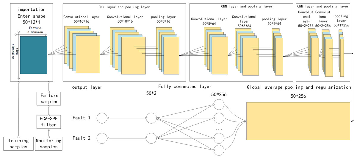
Figure 1: Structure of PCA-SPE-CNN classifier.
The CNN layer involves two primary operations: convolution and activation. The input to the convolution operation is a 3D tensor Z ∈ , where w, h, and c denote the width, height, and number of channels, respectively. In the special case where c = 1, the input simplifies to a 2D form ∈ , which is used as input to the proposed model. Specifically, in the two-dimensional input data, the horizontal axis corresponds to the feature dimension, while the vertical axis represents time, with their scales determined by the number of attributes and the sliding window width, respectively. To clearly describe the convolution operation, four hyperparameters are introduced: the number of convolutional kernels K, kernel size F, stride S, and padding P. To ensure that the output maintains the same shape as the input, the input data ∈ is zero-padded accordingly. As a result, the transformed data ∈ retains the original dimensionality. Following the padding, the convolutional slicing operation is performed as follows:
(18) where : + F represents the operation of extracting the subset located between row and row + F, : + F represents the operation of extracting the subset located between column and column + F, and : represents all the data in the direction of the cutting channel.
The convolution and activation methods presented in this section are based entirely on the framework proposed by Wang & Hu (2025), and start at 1 and change with the number of steps S. According to ( , ), data can be extracted from . Let the convolution kernel be denoted as kernel ∈ , let denote the convolution kernel and the corresponding input subregion. The element-wise multiplication between and is performed, and the result is calculated as follows (Wang & Hu, 2025):
(19)
Accordingly, the output is obtained through the following operation (Wang & Hu, 2025):
(20) In this expression, represents an individual element from the set , and the resulting feature map is constructed from , ordered according to the dimensions and . It is worth noting that
(21)
For each convolutional kernel, a corresponding feature map D is generated. Repeating this operation across all K kernels produces a new three-dimensional output tensor . Following the convolution operation, an activation function is applied to introduce nonlinearity into the network. This nonlinearity enhances the model’s capacity to learn complex representations and improves the separability of features. In this study, the Rectified Linear Unit (ReLU), a widely adopted activation function, is used to activate each element of the output tensor . The activation is defined as Wang & Hu (2025):
(22) Here, denotes an element of , and denotes an element of , representing the values after the activation operation.
Dropout Regularization:
The Dropout layer helps prevent overfitting by randomly setting a subset of input elements to zero during training. This disrupts co-adaptations between neurons and promotes model generalization. The operation of Dropout is mathematically defined as:
(23) where L denotes the input data, p is the dropout rate, and M is a binary mask matrix sampled from a Bernoulli distribution.
Fully Connected Layer (Dense):
The fully connected layer transforms the output from the global average pooling layer into class probabilities using a weight matrix and a bias vector. Its operation is defined by the following formula:
(24) where G represents the result from the global average pooling layer, W is the associated weight matrix, b denotes the bias vector, and ( ) is the activation function used to convert raw outputs into normalized class probabilities.
Fault diagnosis based on expert system
In compressor online monitoring, early anomalies often appear before alarms as parameters exceed allowable limits. This study uses a PCA-SPE-CNN method to detect such signs, based on data from literature and PetroChina’s Gao Ling Station. It analyzes the correlation among abnormal parameters, components, and failure modes. For the recipe positioning compressor, a network-based diagnostic system was developed to process monitoring data and, upon detecting early faults, infer likely failure causes using a knowledge base.
Establishment of knowledge base framework
The causes of faults, troubleshooting methods and their corresponding rule patterns are shown in Table 1 below. The four rules correspond to four faults, namely 1 (compressor vibration or noise), 2 (dry gas seal failure), and 3 (oil pressure too low), 4 (the driver does not start). According to the corresponding inference rules, faults are identified according to the rule with the largest number of matched causes.
| Cause of issue | Correspondence rules | Method of exclusion | |||
|---|---|---|---|---|---|
| Deviation(not corrected) | Yes | No | No | No | Remove the coupling and let the driver run alone. If the driver does not vibrate, the fault may be caused by misalignment. Check the misalignment by referring to the relevant part of the manual. |
| Compressor rotor imbalance | Yes | No | No | No | Check the rotor to see if dirt is causing the imbalance and rebalance if necessary. |
| Bearing wear due to oil contamination | Yes | No | No | No | Check bearings and replace if necessary |
| Coupling unbalanced | Yes | No | No | No | Remove the coupling and check for imbalance |
| Surge | Yes | No | No | No | Whether the compressor operating conditions leave surge conditions |
| Gas contains impurities | No | Yes | No | No | Check filters, replace dirty cores, check pipes are clean |
| Liquid is present in the gas line | No | Yes | No | No | Check the natural gas main pipeline and compressor outlet pipeline |
| Insufficient buffer air pressure | No | Yes | No | No | Check that the pressure difference should not be lower than the specified minimum limit. |
| Insufficient isolation gas pressure | No | Yes | No | No | The pressure should not be lower than the specified minimum limit |
| Dry gas seal gap does not comply with regulations | No | Yes | No | No | The pressure should not be lower than the specified minimum limit |
| There is something wrong with the pump | No | No | Yes | No | The main oil pump does not start: there is no working medium, notify the responsible department. The auxiliary oil pump does not start when the oil pressure drops: electrical failure, electrical failure of the pump automatic equipment (notify the responsible department) |
| Oil pipeline leak | No | No | Yes | No | Leakage at flange connection: seal must be replaced. Oil line rupture hazard: Fire hazard due to contact with hot parts |
| Cooler, filter or strainer is dirty | No | No | Yes | No | Conversion cooler, filter cleaning coarse filter |
| Defective oil pressure balancing valve or pressure reducing valve | No | No | Yes | No | Check valve and replace if necessary |
| Oil pressure is too low | No | No | No | Yes | The pump is defective, the oil pipeline is leaking, the cooler, filter or strainer is dirty, the oil pressure balance valve or pressure reducing valve is defective |
| The oil level in the high tank is too low | No | No | No | Yes | Add enough oil |
| Seal oil pressure difference is too low | No | No | No | Yes | Adjust control valve |
| Oil temperature is too low | No | No | No | Yes | Turn on the heater |
| 1 | 2 | 3 | 4 | ||
Rule mode and fault diagnosis
In order to facilitate the storage of expert knowledge and experience and the corresponding rule relationship in the later maintenance system in the form of documents, the automatic diagnosis mode is mainly based on the improved CNN classifier proposed in this article, and the corresponding rules of the expert system are used to confirm the corresponding faults, and then the follow-up analysis and diagnosis is carried out according to the expert knowledge. Implemented data-driven expert system automatic diagnosis, reducing manual maintenance. Figure 2 shows the automatic confirmation failure mode.
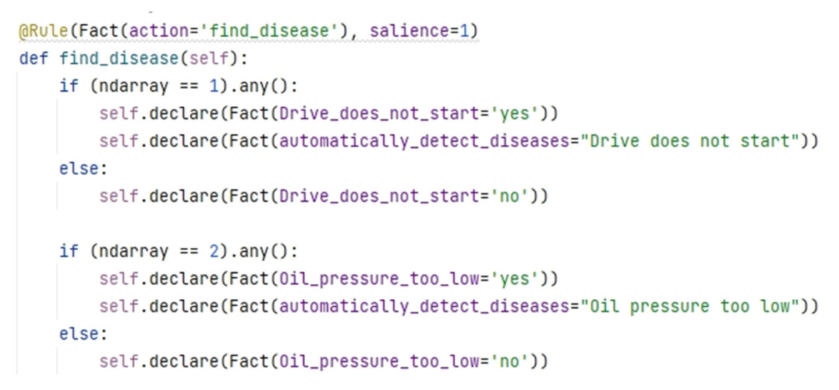
Figure 2: Automatic fault confirmation mode.
If you want to further reason and confirm the detection results, this article adds a manual auxiliary fault detection mode based on expert experience and knowledge. Manual rule reasoning uses the number of corresponding input condition matches to determine the most probable faults based on prior expert knowledge experience and other rule reasoning to determine the most probable faults with the highest number of corresponding input conditions, and Fig. 3 shows the manual confirmation of fault patterns.
Figure 3: Manual matching mode.
The expert system automatically matches the expert experience in the knowledge base based on early automatically identified fault modes to achieve automatic fault diagnosis. The diagnosis results can be used as training data for classifier training, so that it can learn from actual operations, adjust according to the changing environment, and realize automatic updating of the expert system knowledge base. The diagnostic results are shown in Fig. 4 below.
Figure 4: Diagnosis results of low oil pressure.
Analysis of experimental results
Introduction to data settings
For each fault and normal state, the compressor status is represented in both a training data set and a test data set. Each training data set contains 1,500 samples, while each test data set includes 217 samples and corresponding tag data. Each sample consists of 12 features. Therefore, the total number of data points in the original training set is 1,500 × 12 = 18,000, and in the original test set, it is 217 × 12 = 2,604. The data sampling frequency is 1 sample per minute. To ensure effective learning outcomes, the training samples, which include both faulty and normal samples, are randomly shuffled and normalized prior to processing.
Network architecture setup
The input shape of the CNN network is set to a batch size of 50 along the vertical axis, with 12 features along the horizontal axis. The convolution kernels have a size of 1 × 3, and the network employs a series of 16, 16, 64, 64, 256, and 256 convolution kernels. The activation function used is the ReLU function, and the pooling layers include both maximum pooling and average pooling. The network structure consists of three consecutive convolutional layers followed by maximum pooling, with an average pooling layer at the end. To improve performance and prevent overfitting, regularization techniques are applied, and fully connected layers are used for fault classification. The model is trained for 25 epochs, with a total training time of 6 s, which is sufficient to meet the monitoring needs. The hardware reference graphics card is 3,060 or above, the CPU is i5 eighth generation or above, and the hard disk is 50 GB or above.
Parameter tuning
In the data preprocessing stage, we use a sliding window approach to process the monitoring time series. The selection of window length was empirically evaluated by implementing a grid search strategy on the training set, taking into account the sensitivity to transient faults and robustness to noise interference. Classification accuracy and SPE statistical stability were used as measurement criteria to ultimately determine the optimal window length. In addition, during the fault detection phase, residual statistics are obtained via PCA-SPE, with thresholds derived from the chi-square distribution of normal data SPE values. These thresholds are fine-tuned through confidence level adjustments and empirical testing to ensure both consistency and adaptability to varying data distributions.
The network structure is tailored to the nature of the 12-dimensional input, which corresponds to two fault types. A compact convolutional design with small kernels is adopted to emphasize local patterns and hierarchical feature extraction (Wang & Hu, 2025). The architecture, iteratively optimized through experiments, comprises two convolutional layers followed by pooling, supporting better generalization and resilience against noise. To reduce overfitting and strengthen feature learning, regularization techniques and a triple-layer stacking scheme are applied. When stacked across multiple layers, these kernels enable the extraction of broader, high-level features, thereby improving the model’s ability to capture global contextual information (Wang & Hu, 2025). Although larger kernels can directly capture a broader range of features, they require more computational resources, so small kernels are preferred, and the network is deepened to achieve the same results efficiently. This strategy, widely used in successful networks, ensures high computational efficiency. A lower initial learning rate of 0.0002 is chosen, with the Adam optimizer adjusting it during training. A moderate dropout rate of 0.3 is used to prevent overfitting while maintaining model performance, and the number of filters is given an initial value space. Finally, grid search techniques are employed to optimize the model’s parameters, ensuring strong and efficient performance.
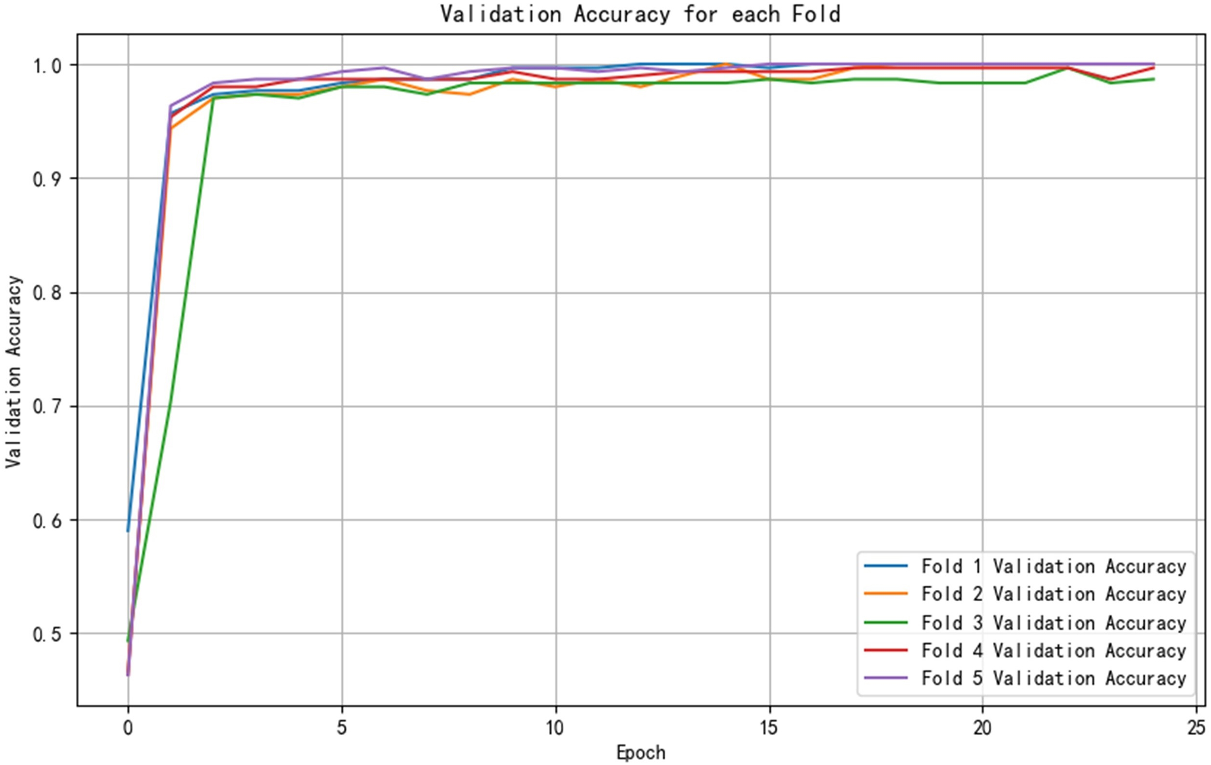
This article uses independently divided training and testing sets, and implements 5-fold cross validation on the training set. Specifically, the train0.csv dataset is divided into five parts, with one part selected as the validation set and the remaining four parts as the training set, while maintaining consistent category distribution. After five rounds of iteration, five sets of training/validation results can be obtained, and their mean (± standard deviation) can be taken as the generalization performance evaluation indicator of the model on the training set. The test set testx1.csv is retained until the final unified evaluation to ensure subject independence, that is, data from the same device/subject will not appear in both the training and testing sets at the same time. The monitoring sample is constructed by dividing the original signal through a sliding window (window length 100, step size 1) and filtering it using the PCA-SPE method. To control the randomness in the experiment, all experiments were fixed with a random seed (seed = 42 in NumPy and TensorFlow), ensuring the reproducibility of the results.
Each experiment was run independently 10 times. The evaluation indicators for model performance include classification accuracy, precision, recall, F1 score, and AUC, and the classification effect is visualized through a confusion matrix.
Classification accuracy and performance analysis of PCA-SPE-CNN classifier
The performance of the PCA-SPE-CNN classifiers has been validated using data, and their performance metrics were comprehensively evaluated. These metrics include accuracy, precision, recall, F1 score, AUC-Receiver Operating Characteristic (ROC), and the ROC curve, all of which were assessed using k-fold cross-validation. The ROC curve, derived from signal detection theory, illustrates the relationship between the true positive rate (TPR) and the false positive rate (FPR) of the classifier, with TPR plotted on the x-axis and FPR on the y-axis. The validation and evaluation results, based on these metrics, are presented and discussed below.
To evaluate classification performance, four key terms are used: true positive (TP), true negative (TN), false positive (FP), and false negative (NP). TP refers to correctly identified positive samples, while TN denotes correctly identified negative samples. FP represents negative samples misclassified as positive, and NP refers to positive samples misclassified as negative. Based on these definitions, the True Positive Rate (TPR) is calculated as TP/(TP + NP), reflecting the proportion of actual positives correctly identified. Similarly, the False Positive Rate (FPR) is FP/(FP + TN), indicating the proportion of actual negatives incorrectly classified as positive.
First, offline normal data is used to train the model. A sliding window is then applied to perform fault monitoring on real-time data. According to Eqs. (12) and (17), the SPE statistic and its corresponding control limit are calculated. Fault detection is conducted by comparing these two values: data points with SPE values exceeding the control limit are identified as faults. The monitoring results are illustrated in Fig. 5. The corresponding normal data filtering part is shown in Fig. 6.
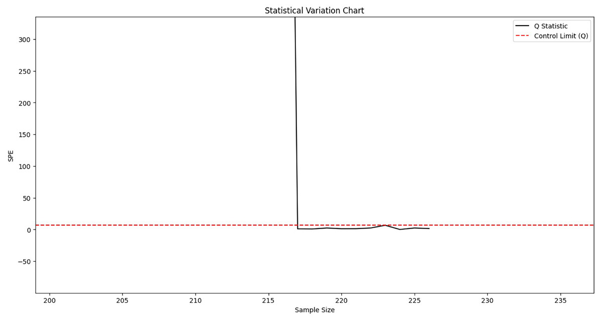
Figure 5: Fault monitoring.
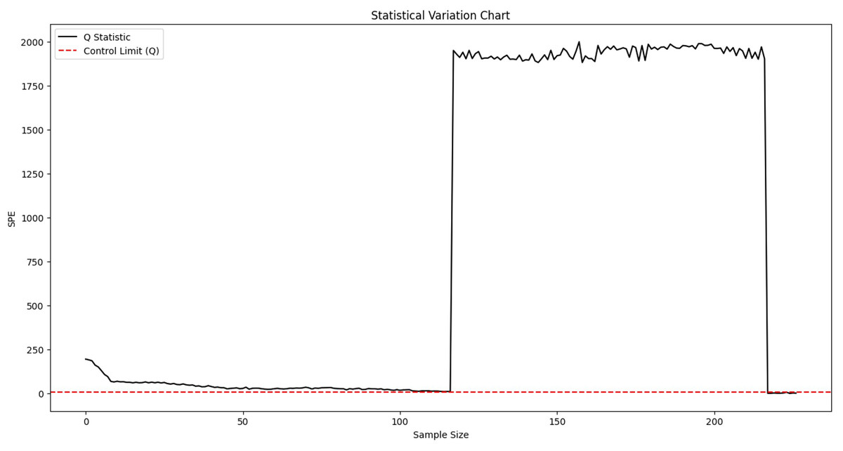
Figure 6: Partial enlargement of normal data monitoring.
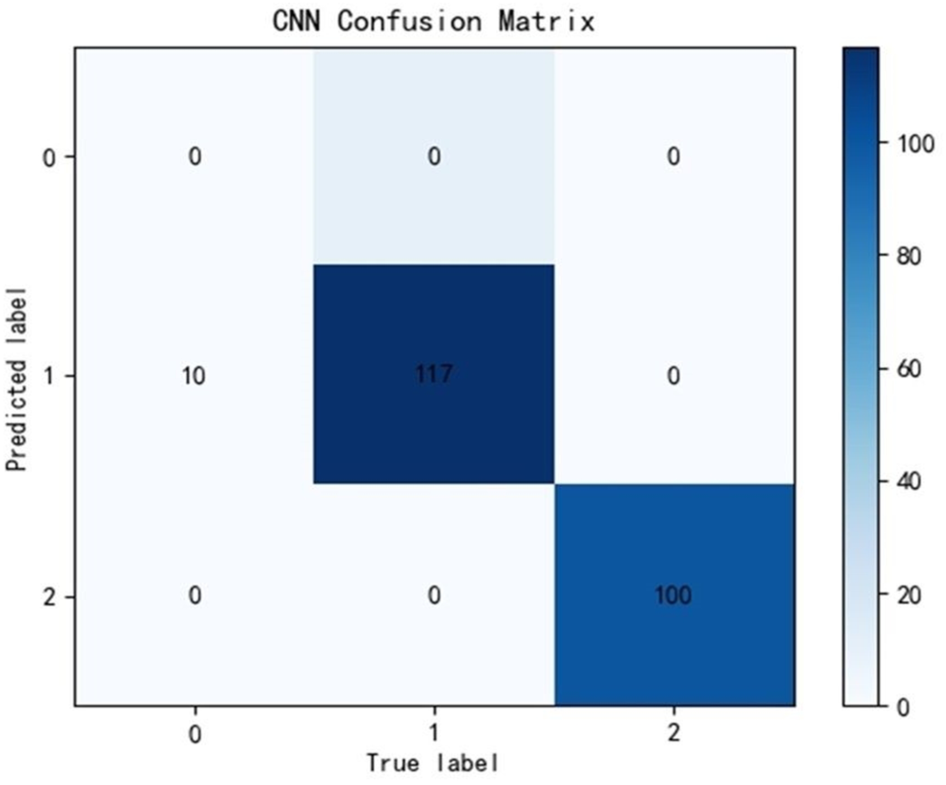
After training the PCA-SPE-CNN algorithm, a confusion matrix was constructed, and the improved algorithm achieved 100% classification accuracy. The classification accuracy for both the training and verification sets, as well as the model’s classification results, are presented in Fig. 7. Additionally, the model underwent an evaluation based on the ROC curve, which is derived from the theory of signal detection. The ROC curve illustrates the relationship between the true positive rate (TPR) and the false positive rate (FPR) of the classifier (with TPR on the x-axis and FPR on the y-axis). This curve reflects the model’s performance across different thresholds, as shown in Fig. 8. The model also underwent k-fold cross-validation, as demonstrated in Fig. 9. To comprehensively assess the model’s performance, an analysis was conducted on various metrics, including accuracy, precision, recall, F1 score, and AUC-ROC. The results of this analysis are presented in Table 2 (Wang & Hu, 2025). Furthermore, the Bootstrap method was applied to estimate the performance metrics, enhancing the robustness of the analysis. By resampling 1,000 times, this method ensured that the model performed consistently under different validation set samples. Finally, the mean and 95% confidence intervals for the performance indicators were calculated to assess the variability in model performance under different sampling conditions. The calculated results are as follows: mean AUC: 1.000, 95% confidence interval (CI) [1.000–1.000]. mean accuracy: 1.00, 95% CI [1.00–1.000].
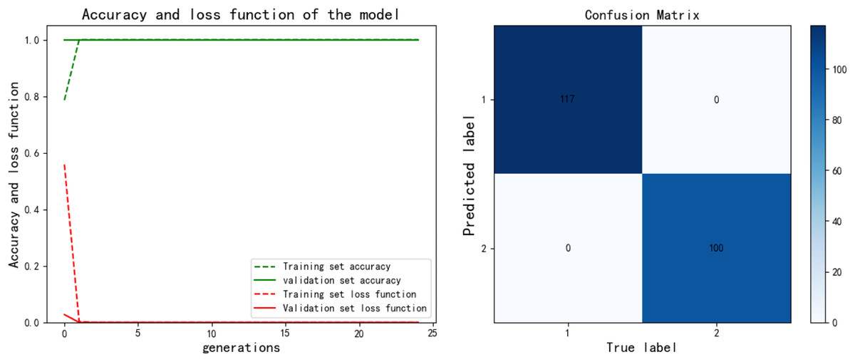
Figure 7: PCA-SPE-CNN classification results.
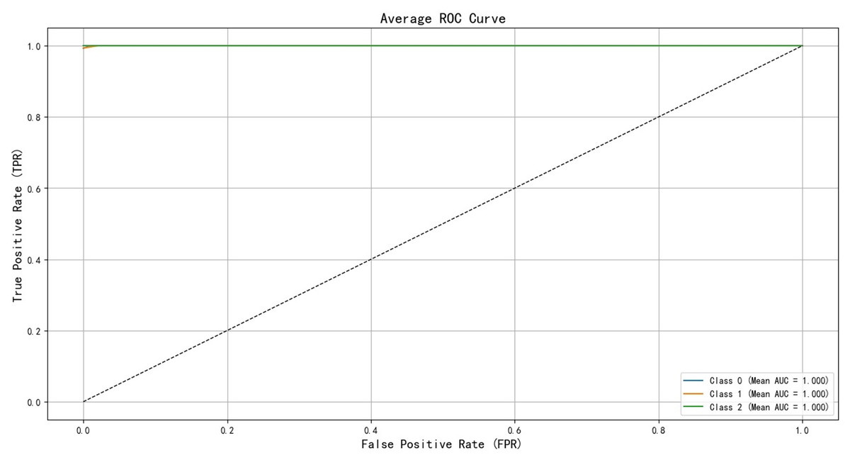
Figure 8: ROC curve of training set validation set.
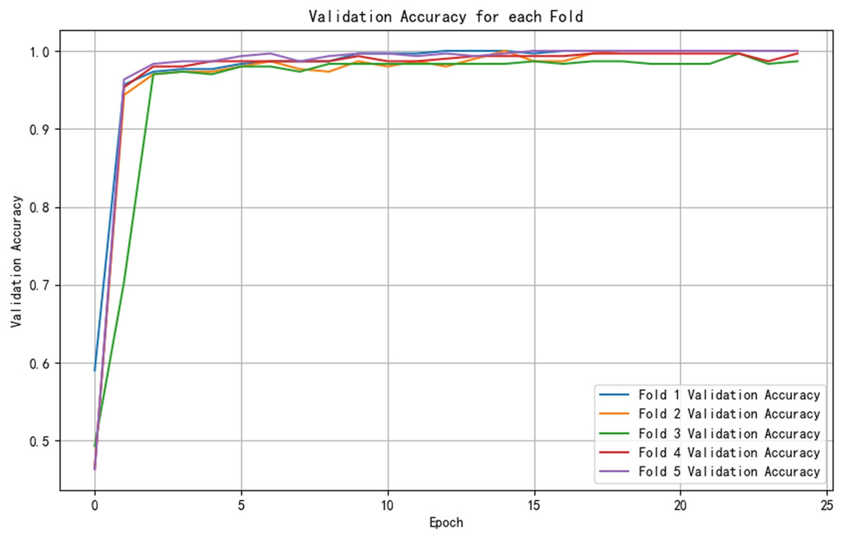
Figure 9: Cross-validation results.
| Index folded number |
Validation accuracy | Accuracy | Precision | Recall | F1-score | AUC-ROC |
|---|---|---|---|---|---|---|
| 1-fold | 1 | 1 | 1 | 1 | 1 | 1 |
| 2-fold | 1 | 1 | 1 | 1 | 1 | 1 |
| 3-fold | 0.997 | 0.987 | 0.987 | 0.987 | 0.987 | 1 |
| 4-fold | 0.997 | 0.997 | 0.997 | 0.997 | 0.997 | 1 |
| 5-fold | 1 | 1 | 1 | 1 | 1 | 1 |
| Mean | 0.998 | 0.997 | 0.997 | 0.997 | 0.997 | 1 |
Mean AUC: this refers to the average AUC value of the model across all Bootstrap resamples. A value closer to 1 indicates better discriminative ability of the model.
95% CI for AUC: The 95% confidence interval for the AUC represents the range in which the model’s AUC value is expected to fall with 95% probability under different resampling conditions. A smaller interval suggests that the model’s performance is relatively stable, while a larger interval indicates significant fluctuations in performance across different data. Mean accuracy: this is the average accuracy of the model’s predictions across all resamples. 95% CI for accuracy: The 95% confidence interval for accuracy shows the fluctuation range of the model’s accuracy under various resampling conditions.
Classification accuracy and performance analysis of three classifiers
Due to the significant differences in the selected data, it is difficult to distinguish between known edge normal data and abnormal data. After training CNN, LSTM, and Transformer algorithms, a confusion matrix was constructed, and complex model comparisons were made through accuracy, precision, recall, and F1 scores. According to the confusion matrix, the classification performance is far inferior to the improved PCA-SPE-CNN model, and the accuracy, recall, and F1 score of the three compared models are not as good as the improved model. Table 3 shows their metric evaluations, while Figs. 10, 11, and 12 present their classification results. By comparing the above, the best solution can be achieved.
| Classifier name | Accuracy | Precision | Recall | F1-score |
|---|---|---|---|---|
| CNN | 0.955 | 1 | 0.953 | 0.973 |
| LSTM | 0.952 | 0.977 | 0.952 | 0.959 |
| Transformer | 0.044 | 0.002 | 0.044 | 0.003 |
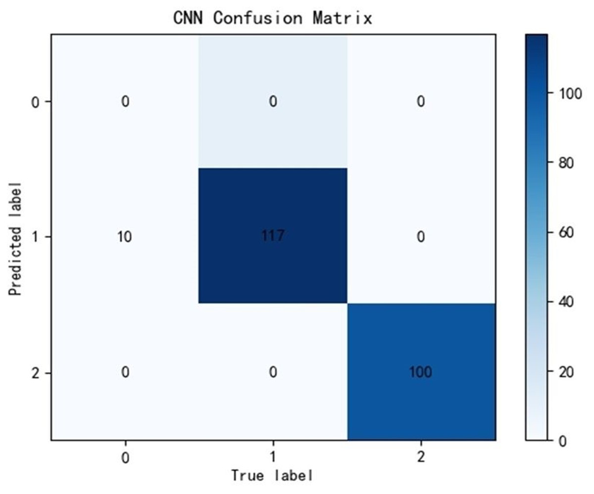
Figure 10: CNN classification results.
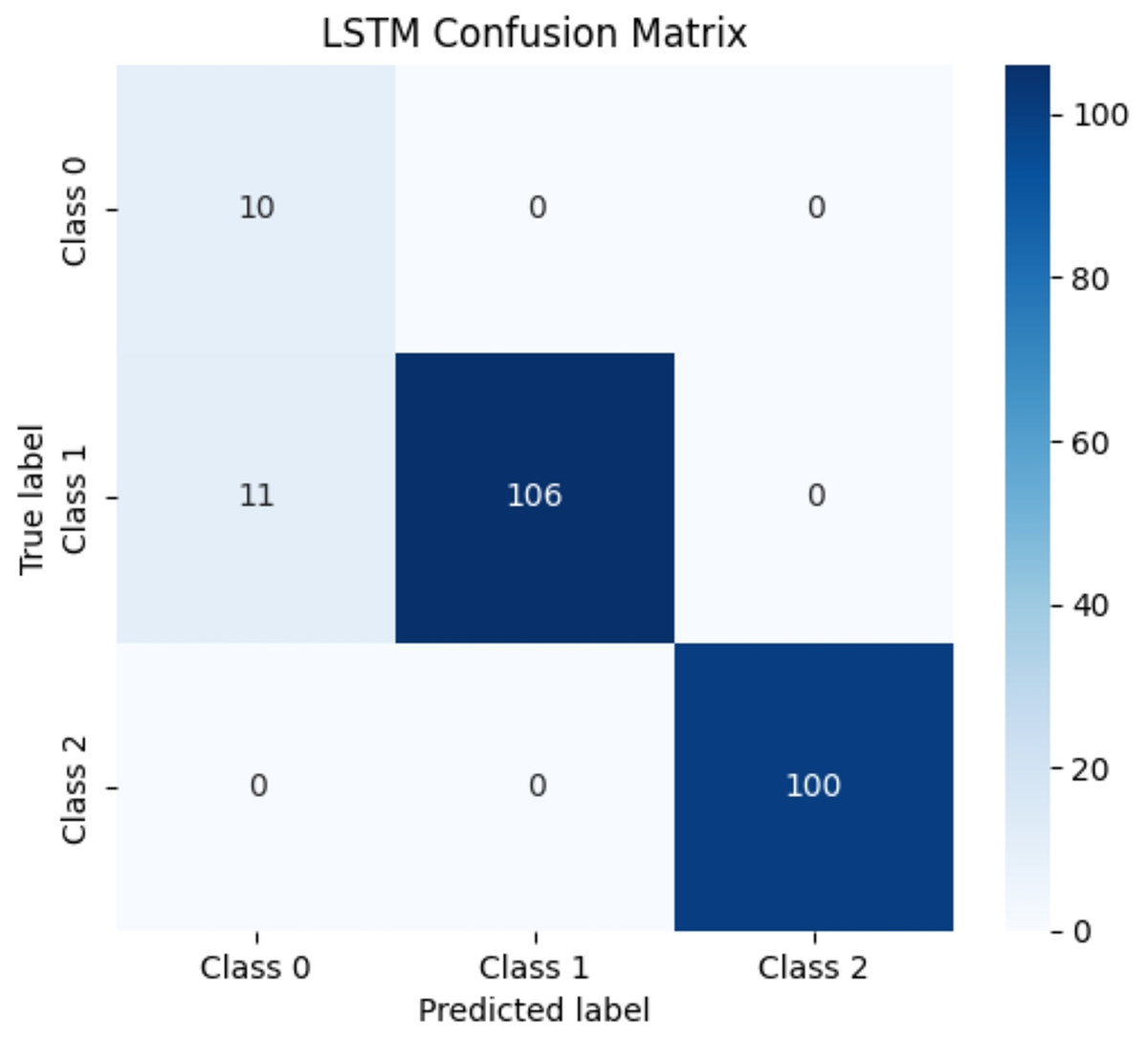
Figure 11: LSTM classification results.
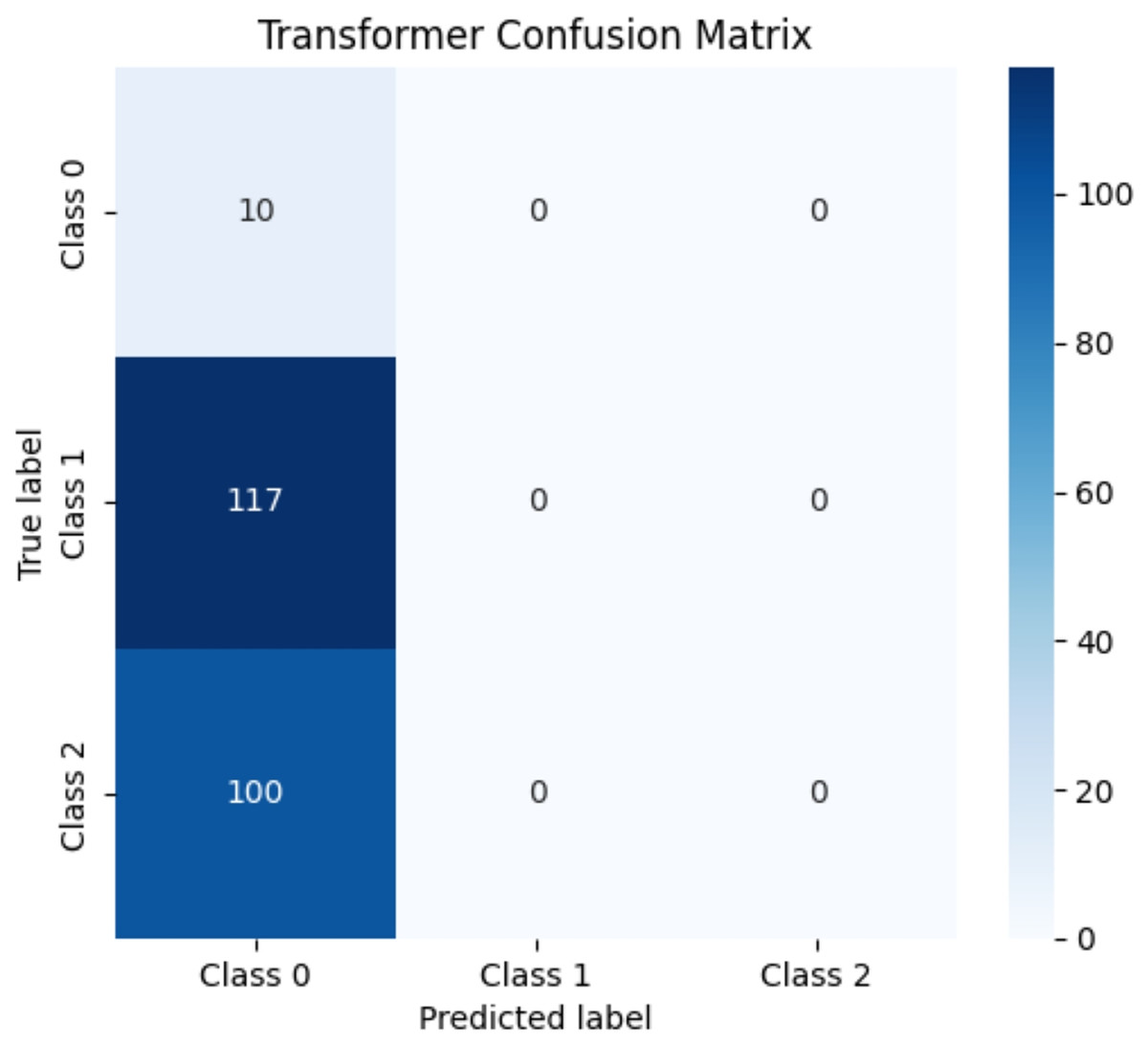
Figure 12: Transformer classification results.
Expert system automatic diagnosis and analysis
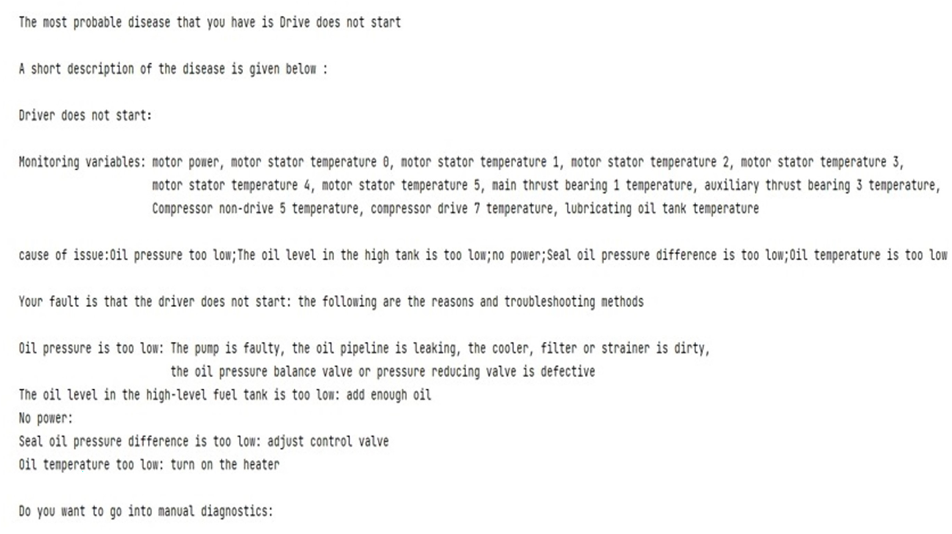
After the new data is input, the system will perform feature matching and pattern recognition to determine whether existing rules are applicable. Apply relevant rules from the rule library to new data through a rule engine to generate new knowledge. Integrate the generated new knowledge with the content in the existing knowledge base to avoid redundancy and maintain consistency. Once the new knowledge is successfully integrated with the existing knowledge base, the system automatically updates the knowledge base without manual intervention. The expert system’s diagnostic results are shown in Fig. 13 below.
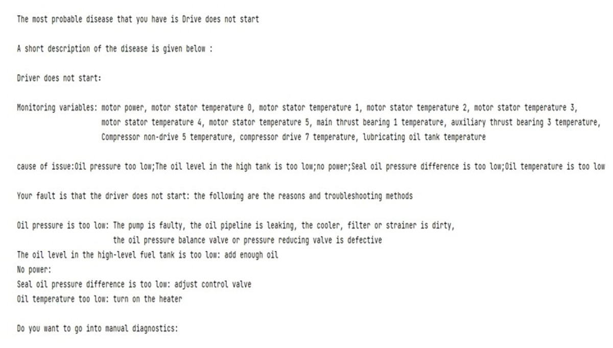
Figure 13: Diagnostic results of driver not starting.
Conclusions
In this article, the performance of the proposed PCA-SPE-CNN classifier is tested based on process data of industrial centrifugal compressors. This classifier is also combined with an expert system to realize the automatic diagnosis of the expert system. This method greatly improves the following problems:
First, it improves the accuracy of fault classification; second, it improves the difficulty of knowledge base maintenance and the lack of flexibility of traditional rule-based fault diagnosis expert systems. The system is able to learn from actual operating data and make adaptive adjustments according to the changing environment, thereby achieving continuous updating of the knowledge base and automatic integration of expert knowledge to effectively diagnose faults. However, this study still has certain limitations. The model’s generalization under extreme operating conditions and across different equipment types requires further verification. Moreover, the current knowledge base has limited capability in modeling and reasoning about complex logical relationships. Future research will explore diagnostic frameworks that integrate knowledge graphs with Graph Neural Networks (GNNs) to achieve deeper fusion of knowledge and enhanced semantic reasoning. By introducing graph-structured knowledge representation and a feature propagation mechanism based on graph convolution, the system is expected to gain stronger causal reasoning and self-learning abilities under complex working conditions. In addition, future work will extend the proposed method to other industrial scenarios to further evaluate its generalization and engineering applicability, thereby providing theoretical and technical support for the continuous evolution of intelligent diagnostic systems.