
TTGNet-AMD: Android malware detection based on multi-modal feature fusion
- Published
- Accepted
- Received
- Academic Editor
- Syed Hassan Shah
- Subject Areas
- Artificial Intelligence, Cryptography, Data Mining and Machine Learning, Data Science, Security and Privacy
- Keywords
- Android malware detection, Opcode sequences, FCG, Feature fusion
- Copyright
- © 2025 Feng et al.
- Licence
- This is an open access article distributed under the terms of the Creative Commons Attribution License, which permits unrestricted use, distribution, reproduction and adaptation in any medium and for any purpose provided that it is properly attributed. For attribution, the original author(s), title, publication source (PeerJ Computer Science) and either DOI or URL of the article must be cited.
- Cite this article
- 2025. TTGNet-AMD: Android malware detection based on multi-modal feature fusion. PeerJ Computer Science 11:e3412 https://doi.org/10.7717/peerj-cs.3412
Abstract
The application of static features for Android malware detection has been extensively studied and developed. Existing methods exhibit limitations in both the completeness and discriminability of feature representation, which affects the enhancement of final classification performance. To achieve a more comprehensive representation of Android software behavior and enhance the detection accuracy, Temporal-Transformer-Graph Network for Android Malware Detection (TTGNet-AMD), a novel multimodal learning model that integrates temporal opcode sequences with structural function call graphs, is proposed for Android malware detection and malware categories classification. This method first extracts the opcode sequence and Function Call Graph (FCG) features, and then prunes and optimizes FCG using the proposed optimization algorithm. Subsequently, both the opcode sequence and the optimized FCG are input into the TTGNet to integrate the two types of features for effective Android malware detection. By utilizing TTGNet, more comprehensive static features of Android software are analyzed, thereby significantly improving the accuracy of malware detection. Finally, the validity of the model was evaluated through extensive experiments in Drebin and CICMalDroid 2020 datasets. The accuracy rate of our method for malware detection is 96.30%, with an F1-score of 94.27%. For malware classification, the accuracy rate is 95.12%, and the F1-score reaches 93.26% respectively.
Introduction
With the continuous upgrading and optimization of mobile devices, the scale of global smart mobile terminal users has shown explosive growth. According to preliminary data from the International Data Corporation (IDC) (International Data Corporation, 2025), global smartphone shipments rose 1.0% year-over-year to 295.2 million units in Q2 2025. Among mobile operating systems, the Android platform has achieved widespread adoption among consumers due to its open-source nature. According to statistics from Counterpoint (2024), as of the second quarter of 2024, Android’s global market share reached 80%, maintaining its leading position in the market. It is worth noting that the rapid expansion of the scale of Android users has also directly promoted the vigorous development of its applications. As of June 2025, there are 1.5 million Android apps in the Google Play Store (Itransition, 2025).
However, the rapid expansion of Android software has concurrently resulted in a significant rise in Android malware. According to the Global Threat Landscape Report (Malware, 2021) released by Statista, malware is showing an explosive growth trend. Between 2015 and 2023, the number of new malware samples increased by 325%, and the total number of malware samples detected worldwide in 2023 exceeded 1.3 billion. According to Google’s report (Itransition, 2025), 2.36 million applications that violated policies were rejected for release on Google Play, and 158,000 developer accounts that attempted to release harmful applications were banned. Malicious software spreads by mimicking legitimate applications, exploiting system vulnerabilities, or through phishing attacks, posing a significant threat to network security. This ongoing deterioration has resulted in substantial economic losses and privacy risks for both end users and businesses. Therefore, enhancing the security protection capabilities of Android applications, especially developing efficient and accurate malware detection technologies, has become a key issue that urgently needs to be addressed in the current field of information security.
Currently, deep learning-based Android malware detection technology has become the mainstream research approach in this field due to its superior feature learning capability and high detection accuracy, and is widely adopted in academic studies. This type of method commonly employs either static feature analysis or dynamic feature analysis to extract effective features. Static feature analysis has become a research hotspot due to its high efficiency and comprehensive feature coverage. Among them, Wang et al. (2014) proposed a method for Android malware detection, PerDroid, based on permission analysis. It selects the top-ranked permissions as features to detect malware. The accuracy of the PerDroid method is 94.01%. However, the accuracy of a single feature is limited, and it is difficult to meet actual needs. Onwuzurike et al. (2017) proposed an Android malware detection method MaMaDroid based on application behavior. It constructs a Markov chain model by abstracting API call sequences to extract features and perform classification. It achieved an accuracy rate and F1-score of 89.6%, with a precision rate of 91.8%. Liu et al. (2024) proposed a novel Android malware detection framework, SeGDroid. They first construct a sensitive function call graph (SFCG) from the original FCG. Then, they combine word2vec and social-network-based centrality measures to extract node attributes, capturing both the semantic knowledge of function calls and the structural properties of the graph. Finally, a graph neural network (GNN) was employed for malware detection. Guan et al. (2020) extracted sensitive APIs corresponding to dangerous permissions and paired them to establish an undirected graph of malicious applications and benign applications. They also assigned different weights based on their importance in malicious and benign applications. Finally, the detection accuracy of malicious applications was 95.44%. However, although the methods mentioned above have achieved certain results, they still have limitations, resulting in insufficient representational ability and discriminative performance. Firstly, the above-mentioned research relies on a single type of feature (such as opcode sequences or function call graphs), which often provides an incomplete view of software behavior. Although opcode sequences can capture chronological patterns, they ignore the structural relationships of the code. Although the function call graph can reflect structural information, it is difficult to express the dynamic context of its execution. Secondly, even if some works attempt to fuse multimodal features, they usually adopt simple feature concatenation or early fusion strategies, failing to achieve deeper and collaborative feature interaction, resulting in limited improvement in the discriminability of the fused features.
In view of the limitation that the current Android malware detection methods have an incomplete representation of software behavior, which impairs the discriminative capability of the detection model, this article proposes TTGNet-AMD, an Android malware detection method based on multimodal feature fusion. The approach first decompiles the APK to extract opcode sequences and function call features separately, then fuses these two feature types, and finally performs Android malware detection and malware category classification using the TTGNet model.
To summarize, the main contributions of this article are outlined in three points.
-
(1)
A multi-type static feature fusion method is proposed. First, the APK is decompiled to extract static opcodes and function call features, with opcodes represented as opcode sequences and function call features encoded as function call graphs. Subsequently, both the opcode sequence and the function call graph are optimized through the proposed algorithms. Finally, the two feature types are fused and jointly represented within the proposed TTGNet-AMD framework.
-
(2)
We propose the TTGNet model for Android malware detection and malware category classification. The TTGNet model learns features from the opcode sequence using LSTM to capture long-term dependencies and local patterns, while enhancing feature representation of function call graphs through Transformer+GCN. Finally, the two types of features are fused to enable accurate Android malware detection and malware category classification.
-
(3)
Systematic and rigorous experimental verification was conducted. Through multiple sets of comparative experiments, the proposed method not only verifies the model’s effectiveness but also performs a benchmark comparison against existing mainstream approaches, thereby demonstrating its superiority.
The rest of the article is organized as follows. We discuss some related work in ‘Related Work’. ‘Methodology’ is arranged to depict our framework. ‘Experiments’ presents our experiment results. ‘Conclusion and Future Work’ concludes this article and points out future directions.
Related work
As the threat of Android malware continues to escalate, its security issues have attracted widespread attention. Researchers have conducted in-depth research in this field and proposed a variety of effective detection methods (Taheri et al., 2020; Ali & Abdul-Qawy, 2021; Ghasempour, Abari & Sani, 2020), making important contributions to the development of Android malware detection technology. The current mainstream detection methods can generally be categorized into three types based on their feature extraction approaches: static analysis, dynamic analysis, and hybrid analysis (Kharnotia & Arora, 2025).
Dynamic analysis enables the acquisition of software’s dynamic behavioral features during execution. However, it not only requires the establishment of a complex sandbox environment but also faces limitations in feature extraction completeness and time efficiency. The hybrid feature analysis method can obtain relatively accurate detection results. However, the resource cost of hybrid feature detection is relatively high, and it takes a long time to complete a full hybrid analysis, which cannot meet the real-time requirements of malware detection.
Static analysis refers to the process of examining an application’s behavior by analyzing its code, structure, resources, and other components without executing the program. This analysis is performed through automated code scanning, eliminating the need for application installation or execution, and offers advantages such as high code coverage and determinism. Consequently, it has garnered significant attention from researchers. In deep learning-based Android malware detection research, static analysis-driven detection methods can be classified into three categories based on feature representation approaches: visual analysis method (Gupta, Sharma & Garg, 2025), text semantic representation (Zhang et al., 2025), and graph representation method (Hei et al., 2024). The summary of previous studies is shown in Table S1.
Visual analysis methods
The visualization analysis method is a technique that encodes the static features of Android applications into a grayscale image feature space and selects a suitable deep learning model for malware detection. Yang et al. (2022) proposed an Android malware code recognition technology based on image features. First, the binary code file in the APK installation package of the Android application is converted into the corresponding graphic file to extract effective image feature information. Then, the convolutional neural network (CNN) is used to complete the recognition and detection of Android malware code. The final accuracy is 95.20%. Yapici (2025) converts Dalvik bytecode files into grayscale images and RGB images, and uses DenseNet121, ResNet50, and ResNeXt50 for malware detection and malware category classification. They achieved average an accuracy rate of 0.987 and an F1-score of 0.986. However, the aforementioned visualization method, when encoding the static features of Android applications into grayscale image space, may result in the loss of some valuable information and impose limitations on feature representation, thereby impacting the performance of malware detection.
Text semantic representation methods
The text semantic representation method is a technology that represents static features as text sequences and then uses deep learning models to detect malware. Jiang et al. (2025) utilized the text features of system Application Programming Interfaces (APIs) and third-party APIs as representations of Android behavior. On this basis, an Android malware detection model based on textCNN was constructed. The experimental results demonstrate that the proposed detection method achieves high performance. Rashid et al. (2025) utilizes text-based features derived from permissions, intents, and API calls in the AndroidManifest file to represent software behavior and employs a deep learning model for Android malware detection. The experimental results demonstrate an accuracy rate of 98.2% in a cross-dataset evaluation involving 15 malware families and 45,000 applications, highlighting the method’s robustness and generalization capability. However, the behavior of application permissions or APIs lacks contextual connections and is vulnerable to being bypassed by malware; meanwhile, the static features used in the above-mentioned methods may not be able to fully capture the multi-dimensional behavior of the software. Especially for complex malware, its behavioral patterns may be difficult to express through a single class feature.
Graph representation methods
The graph representation method is a method that represents the static features of Android applications as a graph structure and uses graph deep learning models to detect malware (Liu et al., 2023). Wang et al. (2025) proposes a heterogeneous-to-homogeneous graph transformation technique that simplifies the structural complexity of the function call graph by focusing on internal function nodes directly related to malicious behaviors while preserving critical malware-related features. Then, they design an SCKDG that prioritizes the student model’s learning requirements through a multi-stage adaptive distillation mechanism. Extensive experiments were conducted on two large-scale datasets. Compared to standard GNN models, their SCKDG method achieves a maximum F1-score improvement of 2.91%. Lu et al. (2024) proposed an Android malware detection model based on the Android function call graph (FCG) and a denoising graph convolutional network (GCN) designed to resist adversarial attacks. To address the threat of adversarial manipulation, the model incorporates a subgraph network (SGN) to extract underlying structural features from the FCG and assess the extent of obfuscation introduced by attack techniques. Experimental results demonstrate that the proposed method achieves an F1-score of 97.1%, outperforming the baseline approach. Shi et al. (2023) proposed a malware detection method named SFCGDroid, which is based on the sensitive function call graph (SFCG). They first extracted SFCG from the FCG. Then, they fed SFCG into a graph convolutional network for malware detection. For experiments on 26,939 Android software datasets, SFCGDroid achieved 98.22% accuracy and 98.20% F1-score. However, relying solely on the function call graph for Android malware detection results in high feature dimensionality and significant computational overhead. Moreover, malicious software can employ various techniques to perturb or distort the FCG structure, thereby evading detection.
To address the issue that a single feature cannot comprehensively depict the behavior of Android software in the above-mentioned methods, this article proposes a multi-modal feature fusion-based Android malware detection method named TTGNet-AMD. This method integrates the features of opcode sequences and function call graphs. FCG provides a global view of the high-level structure of a program and the interaction between modules, while the sequence of opcodes reveals the underlying specific execution logic and behavioral intentions. The combination of the two provides a complete feature representation of Android software and thus can effectively detect Android malware with high accuracy by integrating deep learning models.
Methodology
The overall architecture of TTGNet-AMD, an Android malware detection method that integrates multimodal features, is shown in Fig. 1. It mainly includes data preprocessing, model construction, and malware detection and category classification.
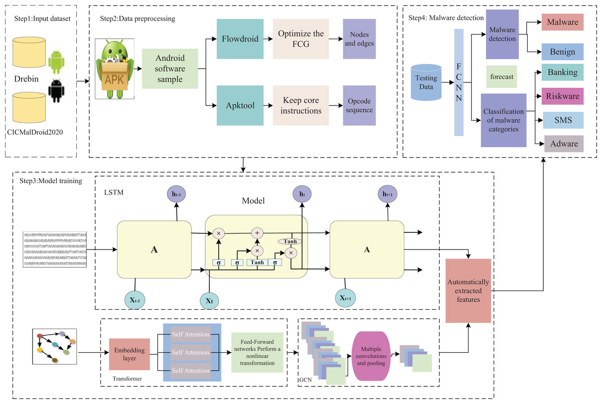
Figure 1: Overall architecture of TTGNet-AMD.
Data preprocessing
Get function call graph features
Function call features (Shi et al., 2023) are the core mechanism for the collaboration between programming languages and computer systems. In essence, a function (caller) executes another function (callee) according to specific rules, and completes control transfer, data transfer, and context management in the process. In Android software analysis, each function name in Android software can be abstracted as a node in a graph structure, and the calling relationship between caller and callee can be modeled as a directed edge to construct a complete function call graph. However, owing to the large scale of Android applications and the highly complex nature of function call behaviors, the constructed function call graphs tend to be intricate. To improve detection efficiency, this study optimizes the function call graph, selects sensitive nodes and edges based on a sensitive API list, and retains only the calling features that have a significant impact on program behavior, which serves as the core basis for Android malware detection. The specific process is as shown in Algorithm 1.
| Input: unoptimized function call graph G; sensitive API list file S |
| Output: pruning rate T; optimized function call graph G(direct overlay) |
| 1. For each Function Call Graph: |
| 2. Read the Call Graph into a graph object G(N, E) |
| 3. Read the sensitive API list file into list S |
| 4. Initialize nodes to remove as an empty list |
| 5. original node count = number of nodes in G |
| 6. For each node N in G: |
| 7. If N is not in S: |
| 8. Get all neighbors of N |
| 9. IF none of the neighbors are in S: |
| 10. Add N to nodes to remove |
| 11. End if |
| 12. End if |
| 13. End for |
| 14. End for |
| 15. Return T, G |
The input of Algorithm 1 is the function call graph and the sensitive API list, and the output is the pruning rate and the optimized function call graph. In the function call graph, nodes are denoted by N and edges by E. Lines 1–5 of Algorithm 1 mainly traverse the function call graph and the sensitive API list file into the graph object G and the list S. Lines 6–13 of Algorithm 1 traverse each node in the graph object G to determine whether it is a sensitive API node and whether all neighboring nodes are sensitive API nodes. If the node is a non-sensitive API node and there are no sensitive API nodes in the neighboring nodes, the node and its adjacent edges are removed. Lines 15 of Algorithm 1 return the pruning rate and the optimized function call graph, respectively.
The comparison of the function call graph before and after call simplification is shown in Fig. S1.
The partial function call graph of the 0a2fcfaef156af4cbb3fb7fde503535dca2fddd07316 bfb59df741118f6f269c.apk malware, which contains 367 edges and 192 nodes. After simplification, it contains 42 edges and 21 nodes, and the simplification rate reaches 88%.
Get opcode sequence features
Opcode features (Tang et al., 2022) refer to instruction-level features extracted from program binary code or intermediate representations (such as bytecodes) to characterize program behavior patterns or functional features. In the process of obtaining opcode sequence features, the original APK file cannot be directly used as training data for the TTGNet-AMD method. Instead, the APK file needs to be parsed by a decompilation tool to extract the classes.dex file. Subsequently, it is converted into a *.smali intermediate code file, and the opcode instruction sequence is extracted from it as the original data feature for subsequent analysis and training. The main steps of preprocessing are shown in Fig. S2.
The Apktool (Dai et al., 2021) tool provided by Google was utilized to decompile the target APK file. During the decompilation process, the main source code files running on the Dalvik virtual machine are obtained, which are Smali format files. Given the huge quantity of Dalvik instructions (including over 200 instructions), this study systematically classifies and optimizes the instruction set to improve analysis efficiency. First, we removed the redundant instructions that were irrelevant to the research objective. Subsequently, we retained a core instruction set along with its corresponding opcode fields. Finally, we stored the screened core instruction set data in a structured text format (.txt) to establish a solid data foundation for subsequent analysis.
TTGNet model construction
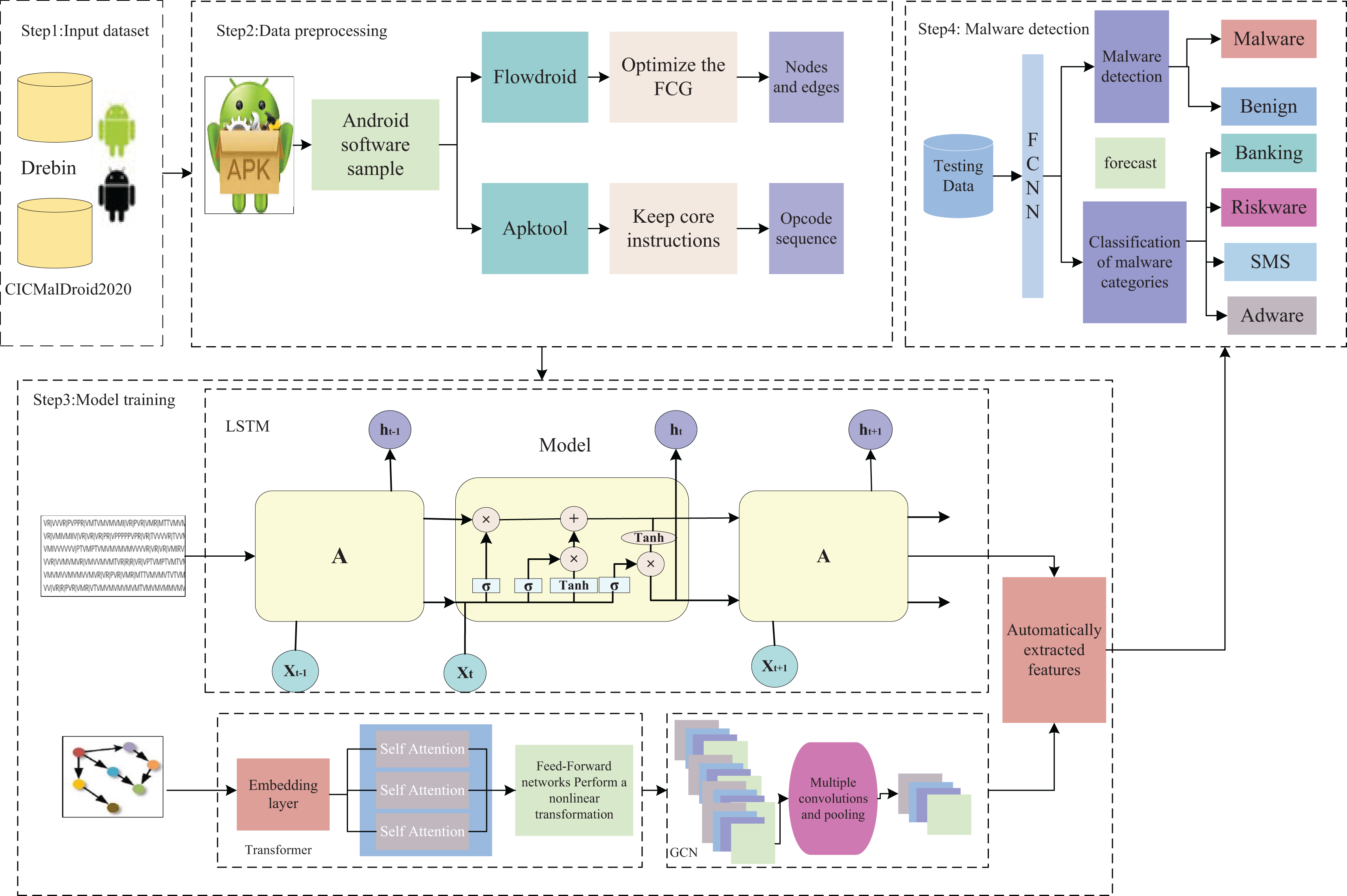
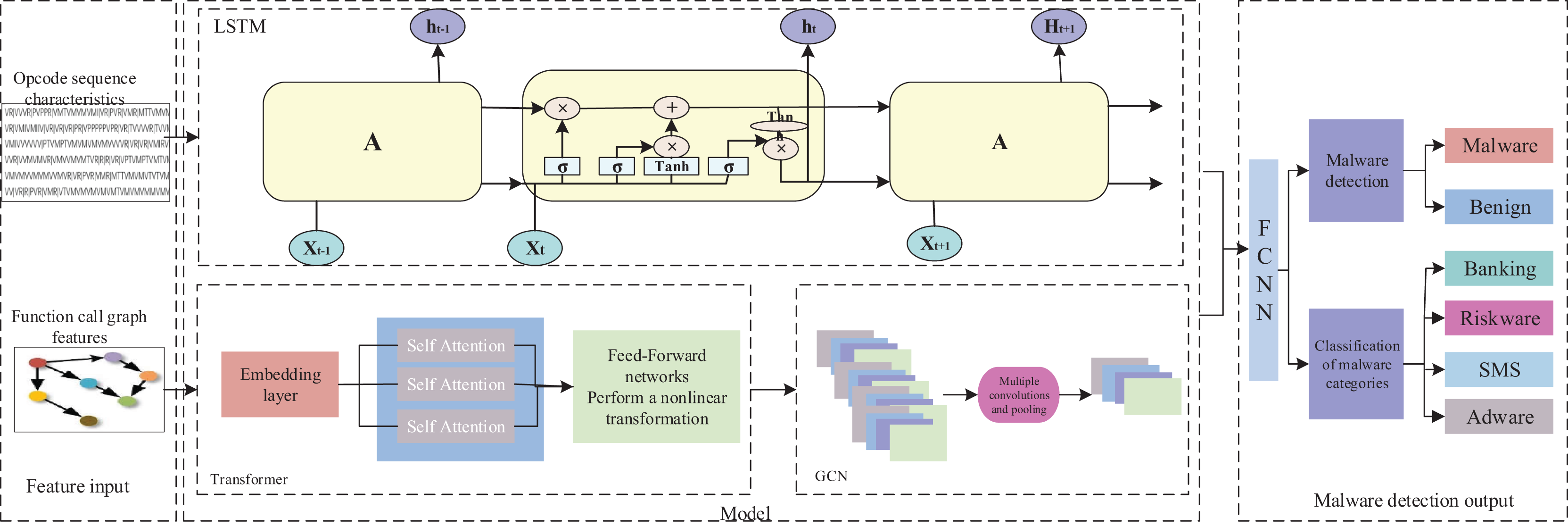
After obtaining the optimized function call graph and opcode sequence features, the TTGNet model extracts the opcode sequence features through the long short-term memory network. The Transformer effectively captures the relationships between long-distance elements in FCG, and the graph convolutional neural network GCN aggregates the node information of function calls, effectively capturing the local structure of the function call relationships. Subsequently, key features are extracted from the opcode sequence and function call graph, and their features are integrated and input into the fully connected neural network for malware detection and malware category classification. The overall TTGNet structure is shown in Fig. 2.
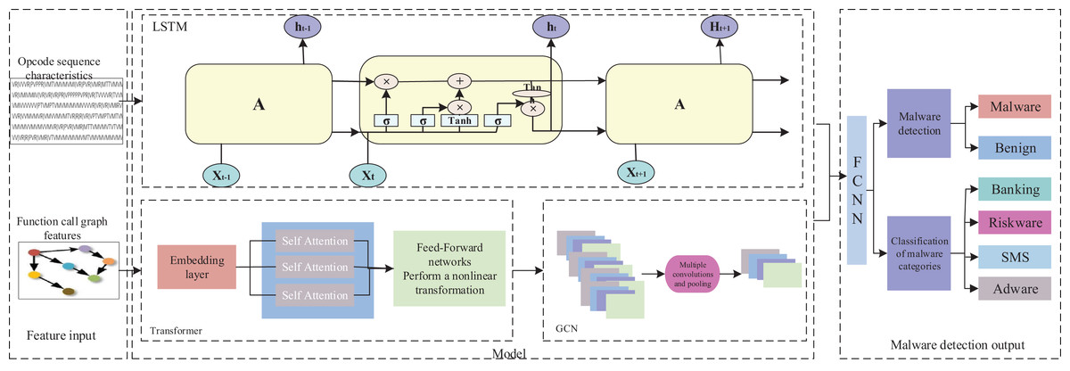
Figure 2: The architecture of TTGNet.
Learning opcode sequence feature models
The long short-term memory (LSTM) network is a special recurrent neural network (RNN) (Liu & Song, 2022) designed to solve the gradient vanishing problem of traditional RNNs when processing long sequence data. LSTM can effectively capture long-distance dependencies by introducing memory cells and gating mechanisms. The core of LSTM is three gating mechanisms (forget gate, input gate, output gate) and a memory cell. The forget gate determines which information is discarded from the memory cell. The opcode sequence feature obtained above is input into the LSTM model, as shown in Eq. (1):
(1)
Among them, is the output of the forget gate, which ranges from 0 to 1. is the weight matrix of the forget gate, is the hidden state of the previous moment, is the input of the current moment, is the bias term of the forget gate, is the sigmoid activation function. The final LSTM model output is a sequence feature, represented by .
The input gate determines which new information is stored in the memory cell, as shown in Eqs. (2) and (3):
(2)
(3) where is the output of the input gate, is the candidate memory cell state, and are the weight matrices of the input gate and candidate state, and and are bias terms.
Next, the memory unit is updated, and the memory unit state is updated through the forget gate and the input gates and . Specifically, as shown in Eq. (4):
(4)
Among them, is the state of the memory unit at the previous moment, and is the state of the memory unit at the current moment.
The output gate determines which information is output from the memory unit to the hidden state. Specifically, as shown in Eqs. (5) and (6):
(5)
(6)
Among them, is the output of the output gate, is the hidden state at the current moment, is the weight matrix of the output gate, and is the bias term.
In the LSTM model, the sigmoid function is the core component of the gating mechanism (input gate, forget gate, and output gate). The output range of the Sigmoid function is [0, 1], which is used to control the passage or forgetting of information. Specifically, as shown in Eq. (7):
(7)
Here, represents the input value, and maps the input to the [0, 1].
The Tanh() activation function is applied in the LSTM model, which is mainly used to perform nonlinear transformation on the values of memory units and hidden states, compressing them into the range of [−1, 1], and enhancing the expressiveness of the model. Specifically, it is shown in Eq. (8):
(8)
Among them, represents the input value, is the exponential growth of input , is the exponential decay of input , determines the output range and shape of the function, is used for normalization, and maps the input to between [−1, 1].
Learning a function call graph feature model
The feature model constructed in this study employs a dual-module cascaded architecture. Firstly, the Transformer-based feature encoding module serializes the representation of the function call graph and leverages its attention mechanism to capture dependencies within the graph. Subsequently, the graph convolutional neural network (GCN) module spatially aggregates the high-order features output by the Transformer, thereby effectively extracting the local structural features of the function call graph.
(1) Transformer
The optimized function call graph features obtained from data preprocessing are input into the Transformer model. The Transformer (Liu & Song, 2022) model is a deep learning architecture based on the self-attention (Lei, Hailin & Yujin, 2014) mechanism. Its core is to dynamically learn the dependencies between input features through the self-attention mechanism, thereby enhancing the significance of key features and suppressing the interference of irrelevant features. The Transformer model consists of four stages: input embedding, encoder, decoder, and output. Each stage is processed by multiple layers of self-attention and feedforward neural networks. The first is the input stage, which includes input embedding and position encoding. The input embedding is a function call graph matrix , used to encode the structured semantic information of the program. Position encoding refers to adding position information to the input sequence, as shown in Eqs. (9) and (10):
(9)
(10)
Among them, and represent the values of the -th dimension and the -th dimension in the positional encoding vector, respectively, represents the position of an element in the input sequence, represents the dimension index of the positional encoding vector, represents the dimension of the positional encoding vector, which is usually the same as the dimension of the input embedding, and is a scaling factor used to control the frequency of different dimensions.
Next is the encoder stage, which is composed of multiple identical layers stacked together. Each layer includes a multi-head self-attention mechanism, a feed-forward neural network, and residual connections and layer normalization. Multi-head attention captures information in different subspaces by calculating multiple self-attention heads in parallel, as shown in Eq. (11):
(11)
The calculation of each attention head is shown in Eq. (12):
(12)
, , denote the query matrix, key matrix, and value matrix, respectively. Among them, , , are obtained by multiplying the input matrix by the corresponding learnable weight matrix , , . , , denote the learnable weight matrix of each head, respectively. denotes the output weight matrix.
The feedforward neural network performs nonlinear transformation on the features of each position, as shown in Eq. (13):
(13)
Among them, , are weight matrices, and , are bias terms.
Residual connection and layer normalization refer to adding residual connection and layer normalization after each sublayer, as shown in Eq. (14):
(14) where is the output of a self-attention or feed-forward neural network, is the output of the final decoder.
Next is the decoder stage, which is also composed of multiple identical layers stacked together. Each layer includes the Masked Multi-Head Self-Attention mechanism, the Encoder-Decoder Attention mechanism, the feedforward neural network, the residual connection, and the layer normalization. The Masked Multi-Head Self-Attention mechanism is used to prevent future information leakage. Its calculation process is similar to that of the Multi-Head Self-Attention mechanism, but the mask matrix is used when calculating the attention score, as shown in Eq. (15):
(15)
Among them, is the final attention score matrix, is the query matrix, is the transpose of the key matrix so that it can be dot-producted with the query matrix, is the dot product of the query vector and the key vector, and the result is an attention score matrix that represents the similarity between each query vector and the key vector, is the dimension of the key vector, is used for scaling to prevent the dot product value from being too large, and the mask matrix is an upper triangular matrix with 0 elements on and below the diagonal and negative infinity above the diagonal to ensure that the current position can only pay attention to the previous position.
The encoder-decoder attention mechanism is used for the decoder to pay attention to the output of the encoder. Its calculation process is similar to the multi-head self-attention mechanism, but the query matrix comes from the decoder, and the key matrix and value matrix come from the encoder. Specifically, as shown in Eq. (16):
(16) where is the hidden state of the decoder and is the output of the encoder.
In the final output stage, the output of the decoder is subjected to a linear transformation to serve as the final output. This is specifically shown in Eq. (17).
(17)
Here, represents the final output, represents the input, represents the weight matrix of the linear layer, and represents the bias term of the linear layer.
-
(2)
Graph convolutional neural network model
Graph convolution neural network (GCN) is a deep learning model for processing graph structured data. It effectively captures the relationship between nodes and their neighboring nodes by aggregating node and neighborhood features and effectively modeling local dependencies. The GCN model structure mainly consists of three parts: input layer, graph convolution layer, and output layer. Use the output of the Transformer as the input of the graph convolutional neural network. The graph convolution operation of each layer is shown in Eq. (18):
(18)
Among them, represents the input feature, , is the adjacency matrix with self-loops added, s is the identity matrix, is the degree matrix of , , is the learning weight matrix of the th layer, and is the activation function. Graph convolution layers usually include multiple layers, and the output of each layer is used as the input of the next layer. Therefore, after multiple graph convolution operations, the output of the last layer can be represented by .
Finally, after multiple graph convolution operations, the output layer outputs the result . The output result j is input into the fully connected neural network for malware detection and category classification.
In the graph convolution operation of the GCN model, the activation function is applied to introduce nonlinear relationships and enhance the expressiveness of the model. Specifically, as shown in Eq. (19):
(19)
Among them, represents the input value. If > 0, output ; if < 0, output 0.
Malware detection model
In the feature extraction stage, the model extracts key features from the opcode sequence and function call graph, respectively, and then fuses these heterogeneous features and inputs them into the fully connected neural network to finally detect malware. The fully connected neural network can learn the complex relationship between input features and output labels by adjusting the weights and biases of the network to complete the classification task. The results and obtained by the above model are used as the input of the fully connected neural network, as shown in Eq. (20):
(20)
Among them, represents the output result, represents the Softmax activation function, represents the learning weight, and represents the bias vector.
In multi-classification problems, the Softmax activation function is usually used in combination with the cross-entropy loss function. The cross-entropy is used to measure the difference between the predicted probability distribution and the true probability distribution. The smaller the value, the better the prediction effect of the model. The advantage of choosing cross-entropy as the loss function is that it has a fast derivation speed and can accelerate network convergence. Specifically, as shown in Eq. (21):
(21)
Among them, m represents the number of samples, k represents the number of classification categories, represents the true classification label of the k-th category of the m-th sample, and represents the predicted classification result of the k-th category of the m-th sample.
When using a fully connected neural network for malware detection, the Softmax function outputs the probability of each category, and the final classification result is determined by the maximum probability. Specifically, as shown in Eq. (22):
(22)
Among them, represents the output result of the function, represents the base of the natural logarithm, represents the i-th element in the input vector, represents the result of the exponential operation of , represents the length of the input vector, and represents the sum of the elements of each input vector after the exponential operation.
Experiments
This section first provides an overview of the datasets and the experimental environment utilized in the study. Secondly, we introduce the data preprocessing procedure and the commonly employed evaluation metrics for the model. Finally, the validity of the proposed TTGNet-AMD model was verified through multiple experimental setups.
Dataset and experimental environment
This subsection primarily describes the two datasets, namely CICMalDroid2020 (Mahdavifar et al., 2020; https://www.unb.ca/cic/datasets/maldroid-2020.html) and Drebin (Arp et al., 2014; https://drebin.mlsec.org/), utilized in the proposed TTGNet-AMD method.
Among them, the Drebin dataset (Arp et al., 2014) comprises 5,560 malicious applications, with sample collection spanning from August 2010 to October 2012. For the experiment, 5,000 of these malicious applications were selected, and 5,000 benign applications were downloaded from the Google Play Store to form a detection dataset. To balance the proportions of the extracted detection dataset, the dataset was divided into training, testing, and validation sets in a 7:2:1 ratio, resulting in 7,000 training samples, 2,000 test samples, and 1,000 validation samples.
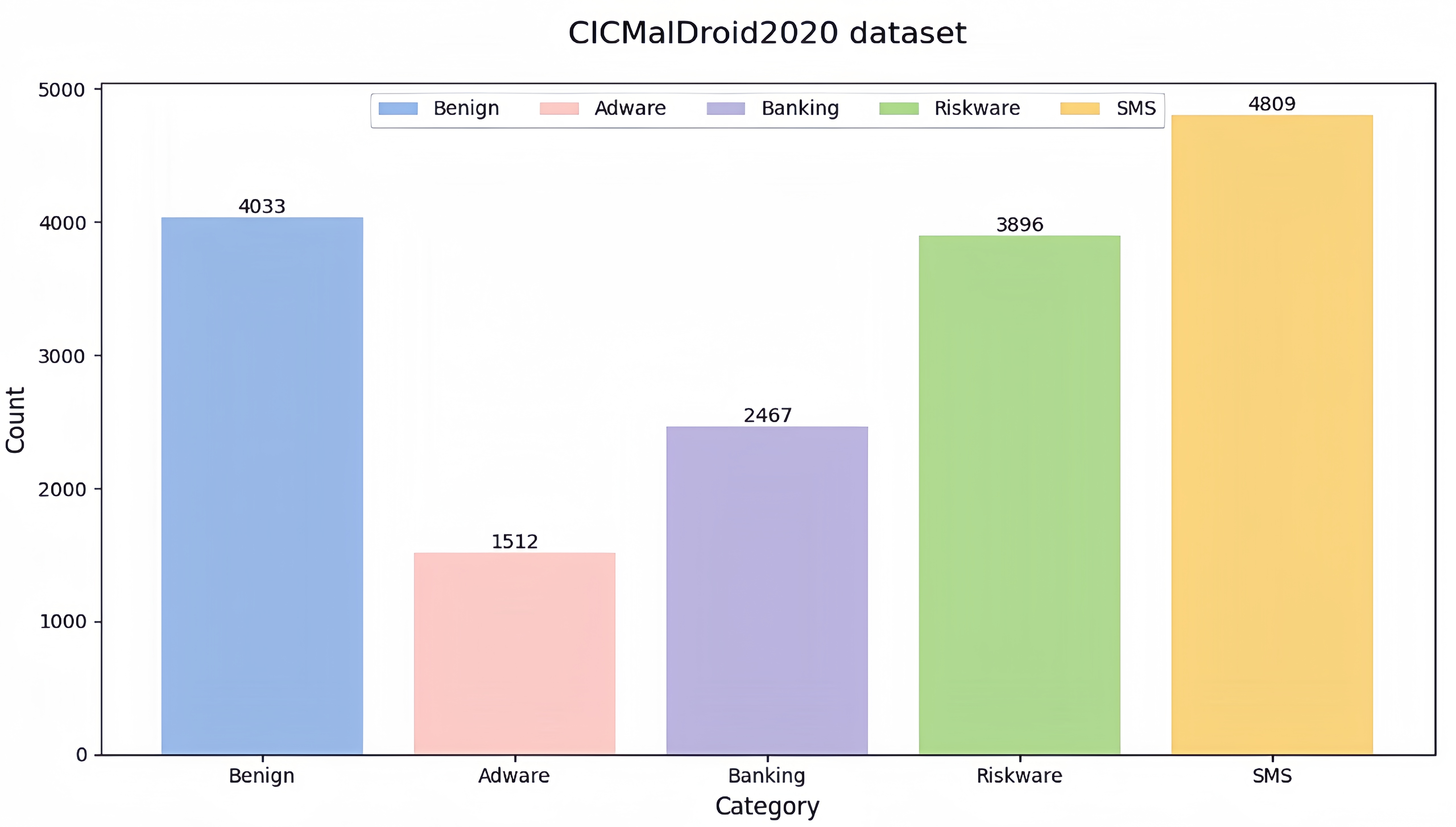
The CICMalDroid2020 dataset comprises Android applications collected by the Canadian Institute for Cybersecurity between December 2017 and December 2018. It includes 4,033 benign applications (Benign), 1,512 adware samples (Adware), 2,467 banking malware instances (Banking Malware), 3,896 mobile riskware cases (Mobile Riskware), and 4,809 SMS malware examples.
The distribution of various software in the CICMalDroid2020 dataset is shown in Fig. S3. The dataset is divided into a training set, a test set, and a validation set in a ratio of 7:2:1. In this experiment, 5,000 benign applications and 5,000 malicious applications were selected from the dataset, resulting in 7,000 training samples, 2,000 test samples, and 1,000 validation samples.
The experiments were conducted under Windows 10 operating system, 128 GB running memory, AMD EPYC 7232P 8-Core Processor CPU, NVIDIA GeForce RTX 3090 GPU, torch 2.4.1, and Python 3.11 environments.
Data preprocessing
The APK files in the CICMalDroid2020 and Drebin datasets are preprocessed to obtain function call graphs and opcode sequence features.
Obtaining function call graph features
We utilize the Flowdroid tool to decompile the APK, extract its function call graph, and optimize the graph based on a predefined list of sensitive APIs. Consequently, the optimized features of the function call graph are obtained. The sensitive APIs list is shown in Table S2. The obtained function call graph and its optimized results are shown in Table S3.
Table S2 presents a list of sensitive APIs, which are primary targets for malware due to their susceptibility to hacking and can consequently disrupt the normal operation of programs. Therefore, this list serves as a critical basis for detecting whether a program has been compromised. Table S3 summarizes the average number of nodes and edges of various function call graph features before and after optimization, along with their optimization rates, thereby specifically illustrating the effectiveness of the optimization method.
Get opcode sequence features
We utilize the Apktool tool to decompile the APK file. During the decompilation process, we extract the primary source code files executed on the Dalvik virtual machine—Smali, and retain only the core instructions within the Smali files. The specific core instructions retained are presented in Table S4.
Subsequently, the extracted function call graph and opcode sequence features are represented in terms of text semantics. Thereafter, these features are utilized as input for the TTGNet model to perform experiments on malware detection and category classification.
Evaluation metrics
For Android malware detection classifiers, the most common evaluation metrics include: true positives (TP), false positives (FP), true negatives (TN), and false negatives (FN). The detailed descriptions of these four metrics are shown in Table S5.
A good Android malicious application detection model should accurately identify malicious applications and reduce the false positive rate. However, the above assumptions cannot fully evaluate the pros and cons of the model in classification. Accuracy, precision, recall, and F1-score are also introduced to evaluate the model, which are shown in Eqs. (23)–(26).
(23)
(24)
(25)
(26)
Experimental results and analysis
This section presents experiments and analyses conducted on malware detection and malware category classification. ‘Android Malware Detection Results and Analysis’ primarily reports the malware detection results achieved by the proposed TTGNet-AMD method. ‘Malware Category Classification Results and Analysis’ details the malware category classification results obtained using the TTGNet-AMD method. ‘Ablation experiment’ validates the effectiveness of each component of the model through ablation studies. ‘Comparison with Other Deep Learning Models and Methods’ provides a comparison of the proposed method with other deep learning models and approaches.
Android malware detection results and analysis
This subsection provides a detailed elaboration of the malware detection results achieved through the proposed TTGNet-AMD.
The experiment utilized two authoritative datasets, CICMalDroid2020 and Drebin, as benchmark testing platforms. A binary classification task was employed to categorize the samples into benign software and malicious software. Regarding parameter configuration, the padding parameter was set to 0, the number of training epochs was set to 100, the initial learning rate was configured as 0.001, and the Adam optimizer (Sivaranjani, Sasikumar & Sugitha, 2025) was selected for optimizing the model parameters.
The detailed performance evaluation results of the experiment are shown in Fig. 3.
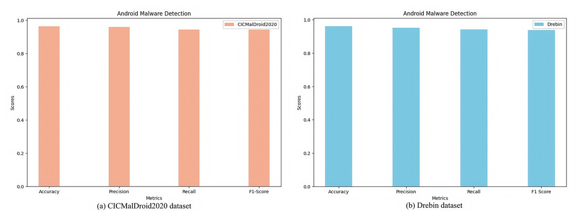
Figure 3: Malware detection results on different datasets.
(A) CICMalDroid2020 dataset. (B) Drebin dataset.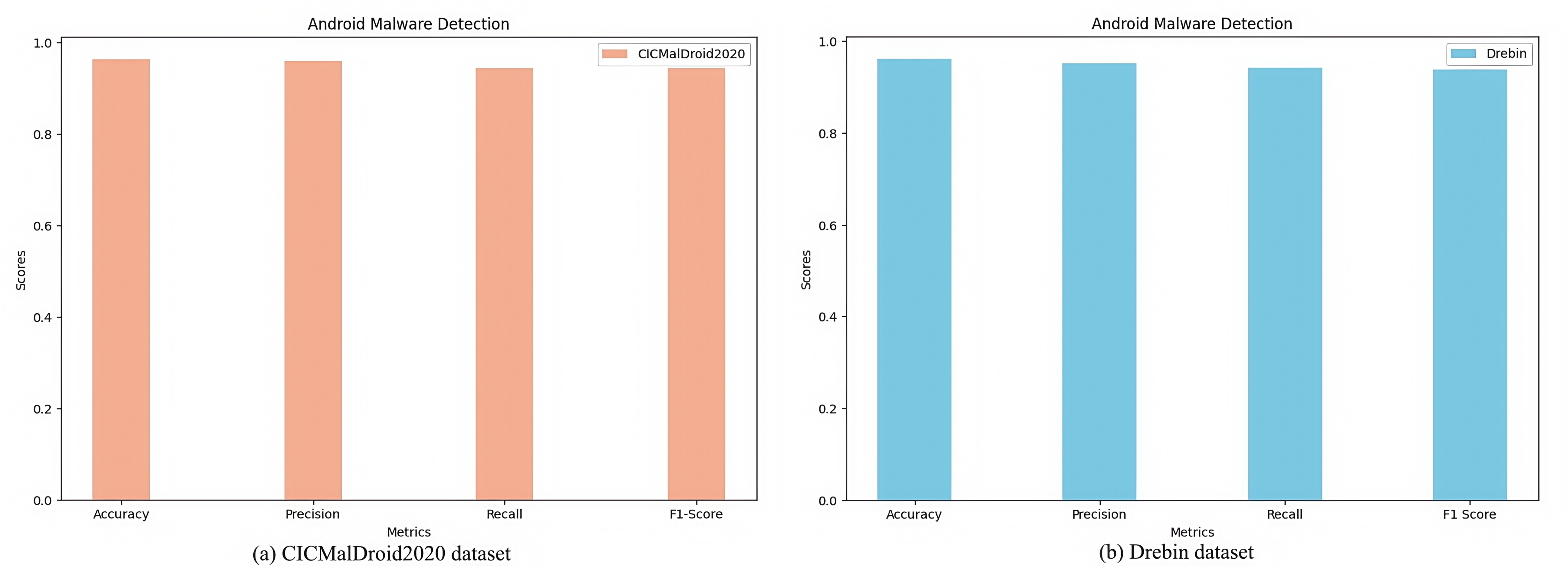
Fig. 3A illustrates the experimental outcomes of the TTGNet-AMD method for Android malware detection on the CICMalDroid2020 dataset, achieving an accuracy of 96.30%, precision of 95.76%, recall of 94.33%, and F1-score of 94.27%. Figure 3B presents the performance metrics of the TTGNet-AMD method for Android malware detection on the Drebin dataset, where the proposed method attains an accuracy of 96.13%, precision of 95.20%, recall of 94.12%, and F1-score of 93.85%.
These results confirm that the proposed TTGNet-AMD achieves high detection accuracy and precision on both datasets, thereby validating the effectiveness and reliability of the model. Furthermore, these findings suggest that the TTGNet-AMD possesses strong generalization capabilities.
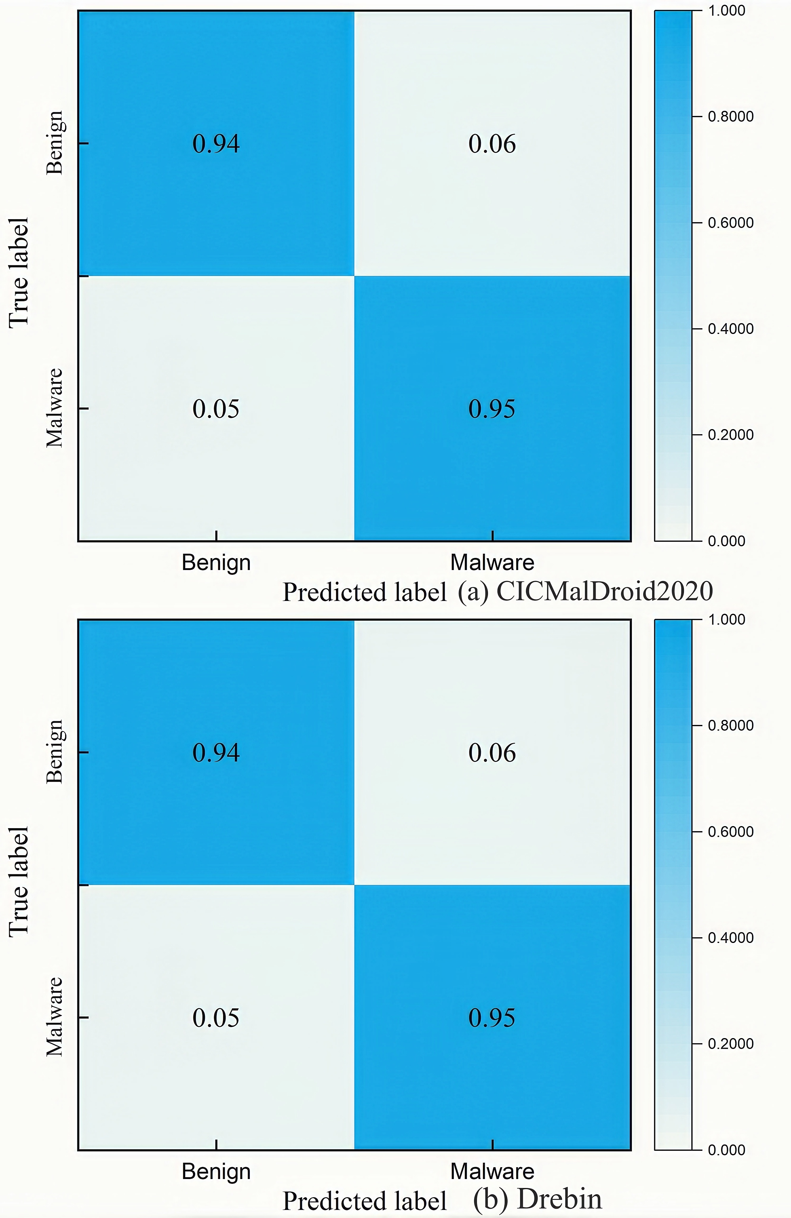
As an important tool for evaluating the performance of classification models, the confusion matrix intuitively displays the correspondence between the prediction results and the true labels. The X-axis of the matrix represents the predicted label, and the Y-axis represents the true label. Figure S4 shows the confusion matrix evaluation results of the TTGNet-AMD method on the CICMalDroid2020 and Drebin datasets.
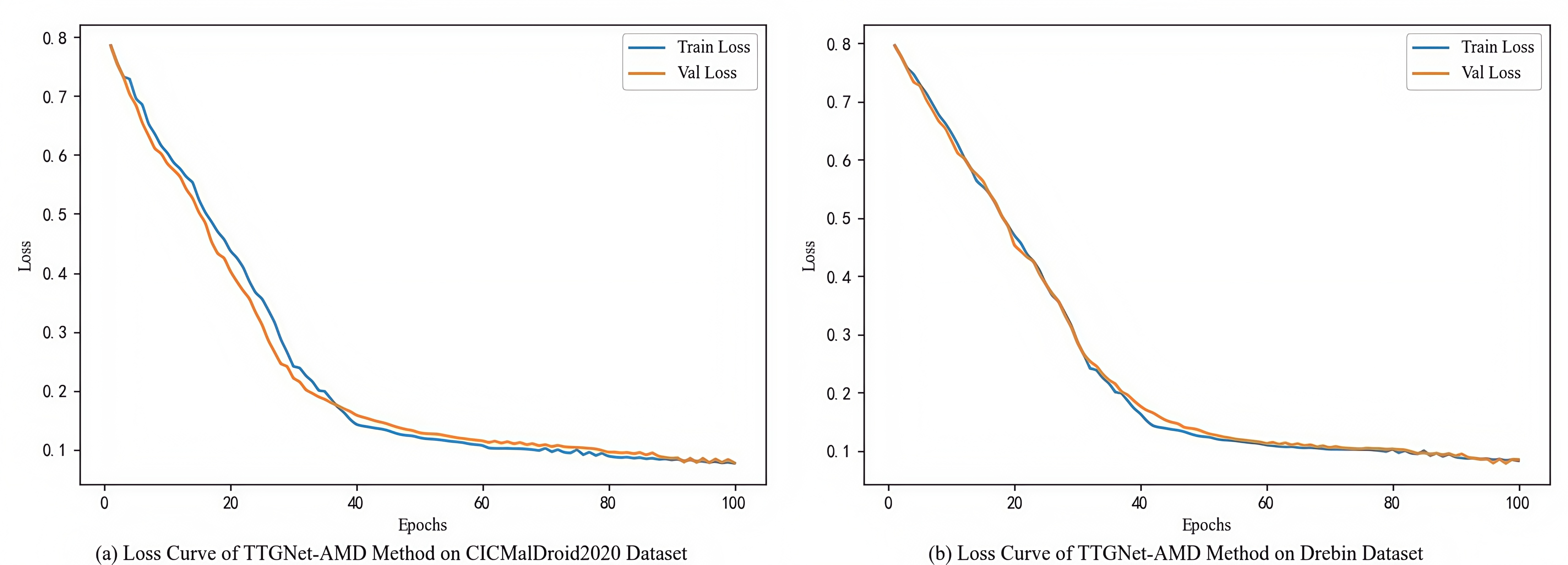
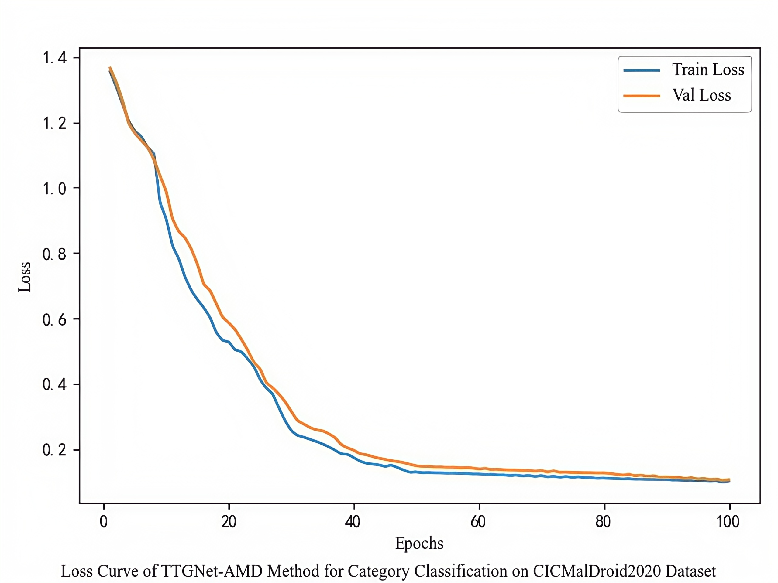
The loss function curve illustrates the evolution of training and validation losses across training epochs. Figure S5 presents the loss curves of the TTGNet-AMD method on the CICMalDroid2020 and Drebin datasets.
The results of training the model on the CICMalDroid2020 dataset and evaluating it on the two datasets as an independent test set are presented in Table 1.
| Different datasets | Evaluation indicators | |||
|---|---|---|---|---|
| Accuracy (%) | Precision (%) | Recall (%) | F1-score (%) | |
| CICMalDroid2020 | 96.30 | 95.76 | 94.33 | 94.27 |
| Drebin | 95.62 | 94.24 | 93.51 | 93.42 |
As shown in Table 1, TTGNet-AMD achieves binary malicious app detection performance with an accuracy of 96.30%, precision of 95.76%, recall of 94.33%, and F1-score of 94.27% on the CICMalDroid2020 test set. When tested on the Drebin dataset, the model maintains strong performance, achieving an accuracy of 95.62%, precision of 94.24%, recall of 93.51%, and F1-score of 93.42%.
Malware category classification results and analysis
This section presents the experimental evaluation results of fine-grained classification of malware categories. The study uses a four-classification task to classify malware samples into four typical categories: Adware, Banking, SMS, and Riskware. This article presents the experimental results of the proposed method for classifying malicious software categories on the CICMalDroid2020 dataset. To comprehensively evaluate the model’s performance, the experiment employs Macro- and Micro-averaged metrics and the confusion matrices. The experimental parameters are configured consistently with those used in the malware detection section. As specifically illustrated in Fig. 4.
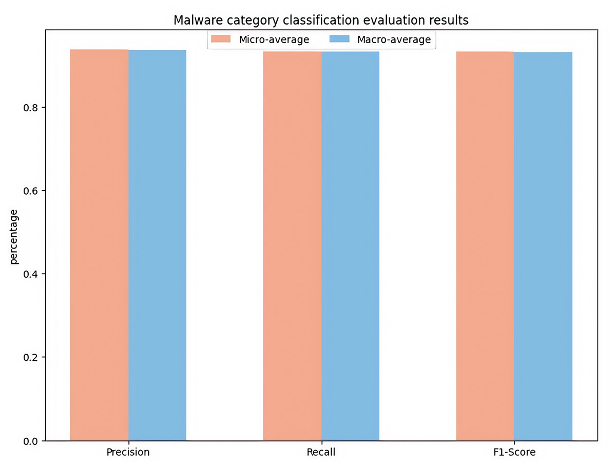
Figure 4: Malware category classification evaluation results.
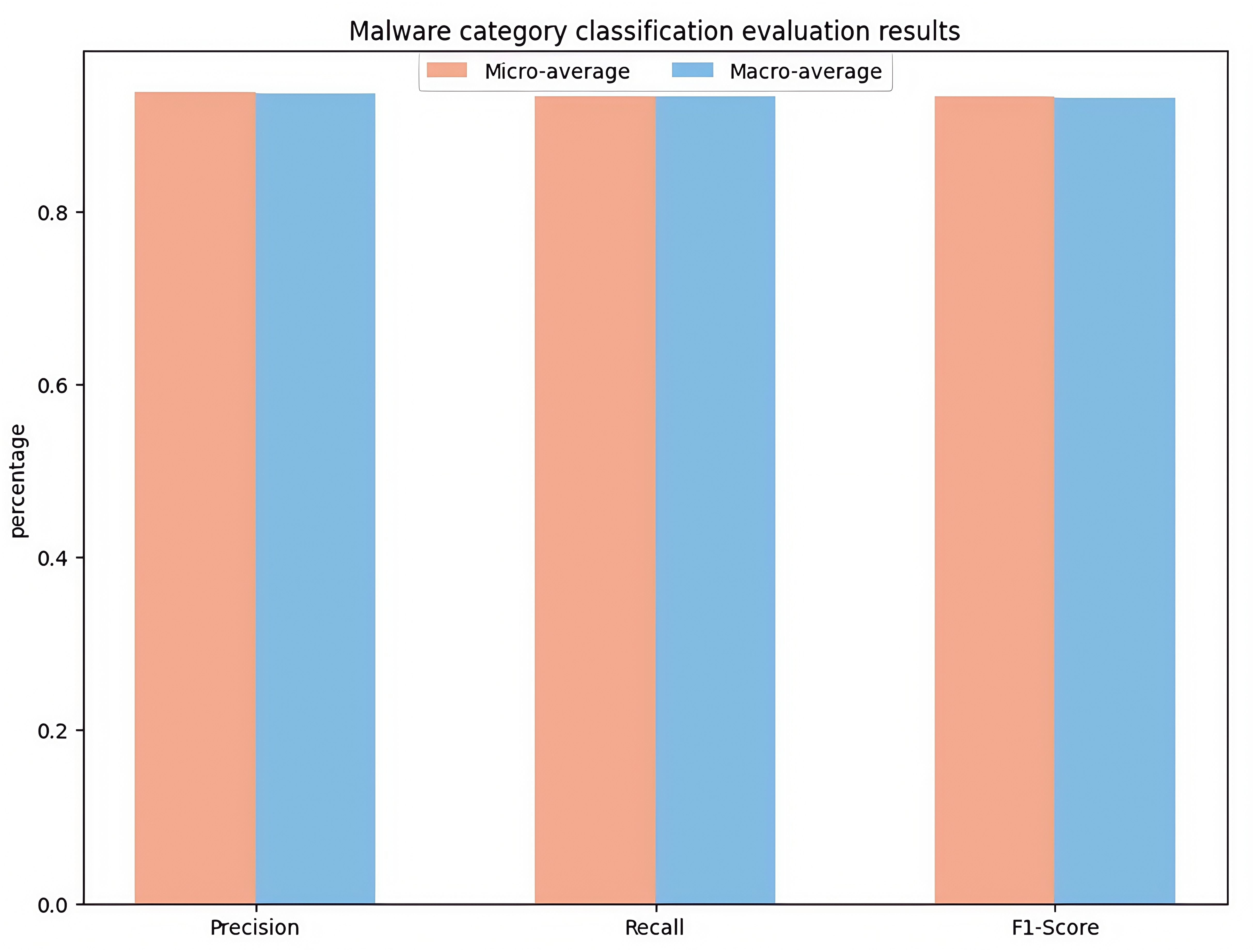
Figure 4 shows the performance evaluation results of four classification tasks (Adware, Banking, Riskware, SMS). The Micro-Precision achieved 93.85%, while the Macro-Precision reached 93.68%, indicating that the model’s prediction results are highly reliable. The Micro-Recall attained 93.31%, and the Macro-Recall was 93.25%, validating the model’s effective recognition capability across various categories of samples. The Micro-F1-score was 93.26%, and the Macro-F1-score was 93.12%, demonstrating a well-balanced trade-off between precision and recall. The overall accuracy of the model was 95.13%, which fully substantiates the effectiveness of the proposed TTGNet-AMD method in fine-grained malicious software classification tasks. These experimental results confirm that the model possesses strong classification capabilities.
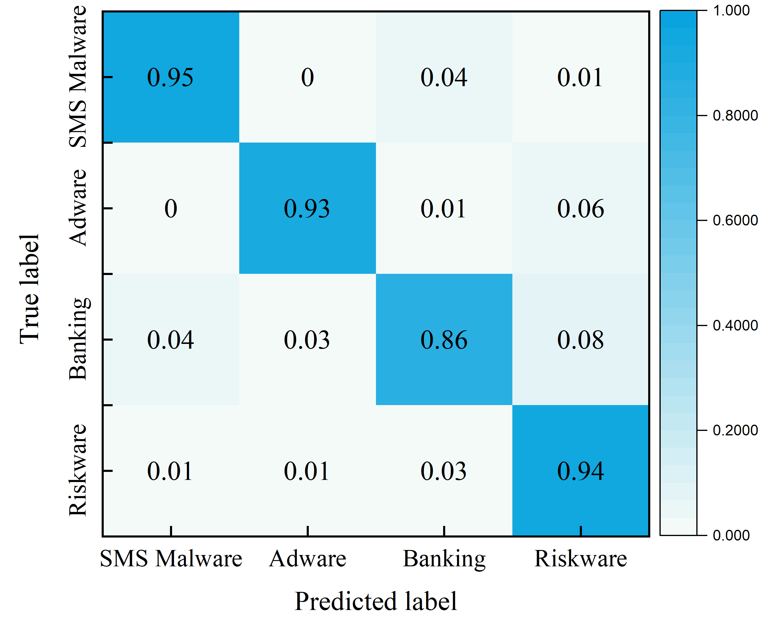
The confusion matrix for the malware category classification experiment using the proposed TTGNet-AMD method on the CICMalDroid2020 dataset is presented in Fig. S6. And the loss curve is shown in Fig. S7.
These results show that the proposed method has the best recognition ability for SMS and Riskware malware, while the recognition performance for Banking samples is relatively weak, which provides a clear direction for subsequent model optimization.
Ablation experiment
This subsection presents the experimental results of malware detection and malware category classification using GCN, Transformer+GCN, and TTGNet-AMD (LSTM+Transformer+GCN) on the CICMalDroid2020 and Drebin datasets. The parameter configurations for each model are consistent with those described in the preceding two subsections. Ultimately, the models’ performance is assessed using evaluation metrics such as accuracy, precision, recall, F1-score, confusion matrix, and AUC curve.
The specific results of the malware detection experiments performed by the three models on the CICMalDroid2020 and Drebin datasets are presented in Fig. 5.
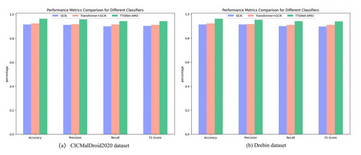
Figure 5: Malware detection evaluation results on different datasets.
(A) CICMalDroid2020 dataset. (B) Drebin dataset.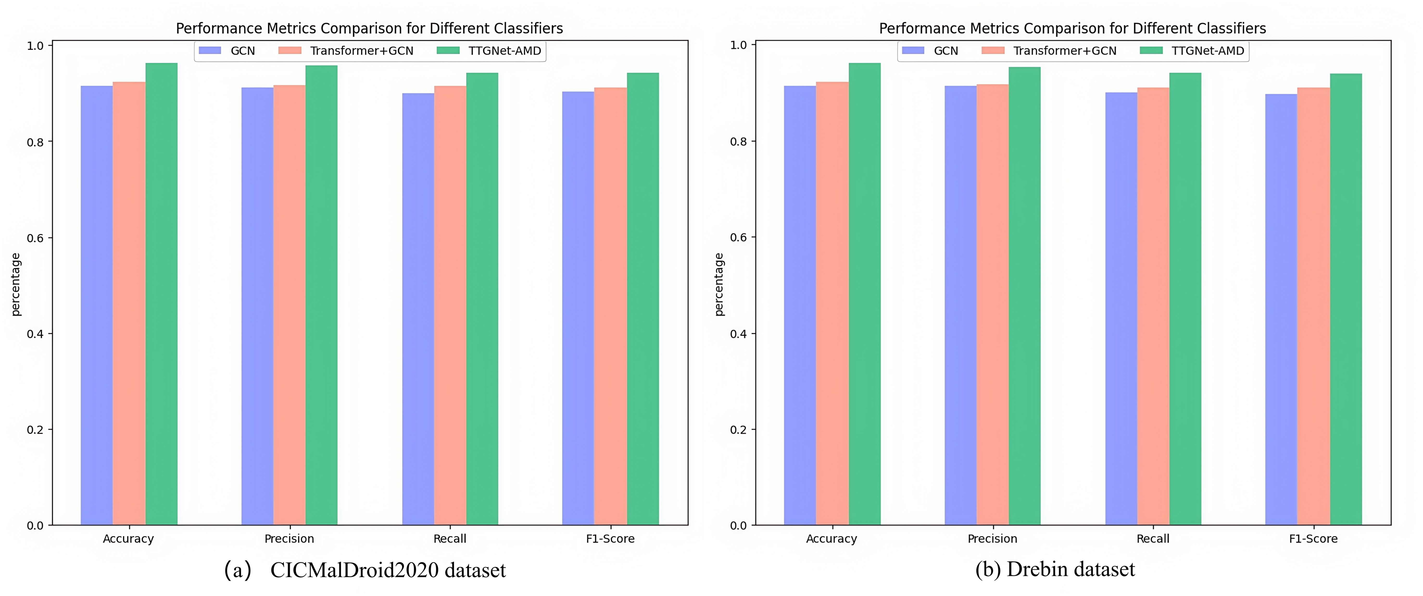
Figure 5 illustrates the performance comparison of three models on the CICMalDroid2020 and Drebin datasets. The experimental results indicate that the malware detection model based solely on the GCN architecture achieved a comprehensive performance index ranging from 90% to 92% on the CICMalDroid2020 dataset, while its performance on the Drebin dataset was slightly lower, varying between 89% and 92%. Upon introducing the Transformer module, the model’s performance improved marginally, with all metrics increasing by approximately 1% to 2% across both datasets. Notably, the hybrid model constructed by further integrating the LSTM module exhibited substantial performance improvements: on the CICMalDroid2020 dataset, the accuracy, precision, recall, and F1-score were enhanced to 96.30%, 95.76%, 94.33%, and 94.27%, respectively; on the Drebin dataset, the corresponding metrics reached 92.35%, 91.65%, 91.03%, and 91.03%.
In conclusion, compared with detection methods based solely on a single feature, employing a multi-feature fusion strategy can more comprehensively capture the behavioral patterns and structural features of malicious software, thereby substantially enhancing detection performance.
The specific results of the malware category classification experiment of the three models on the CICMalDroid2020 dataset are shown in Fig. 6.
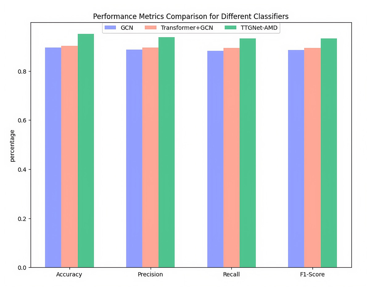
Figure 6: Malware category classification evaluation metrics on the CICMalDroid2020.
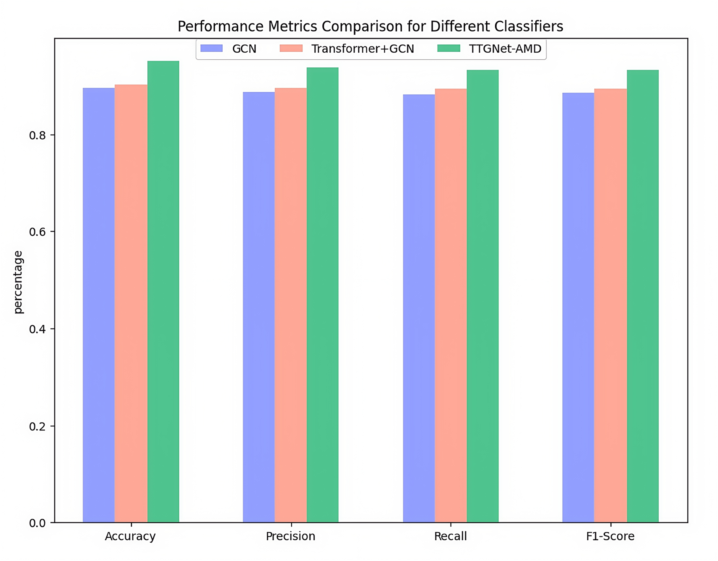
As can be seen from Fig. 6, the single-feature GCN model has an accuracy of 89.62%, a precision of 88.74%, a recall of 88.14%, and an F1-score of 88.62%. The four indicators perform well, but there is still some room for optimization; the performance improvement of the Transformer+GCN combination model is limited, and the four evaluation indicators reach 90.23%, 89.52%, 89.35% and 89.37% respectively, indicating that the improvement effect of introducing only the attention mechanism is weak; the TTGNet-AMD method performs best, and various indicators are significantly improved, namely Accuracy 95.13%, Precision 93.85%, Recall 93.31% and F1-Score 93.26%, indicating the effectiveness of the proposed TTGNet-AMD method.
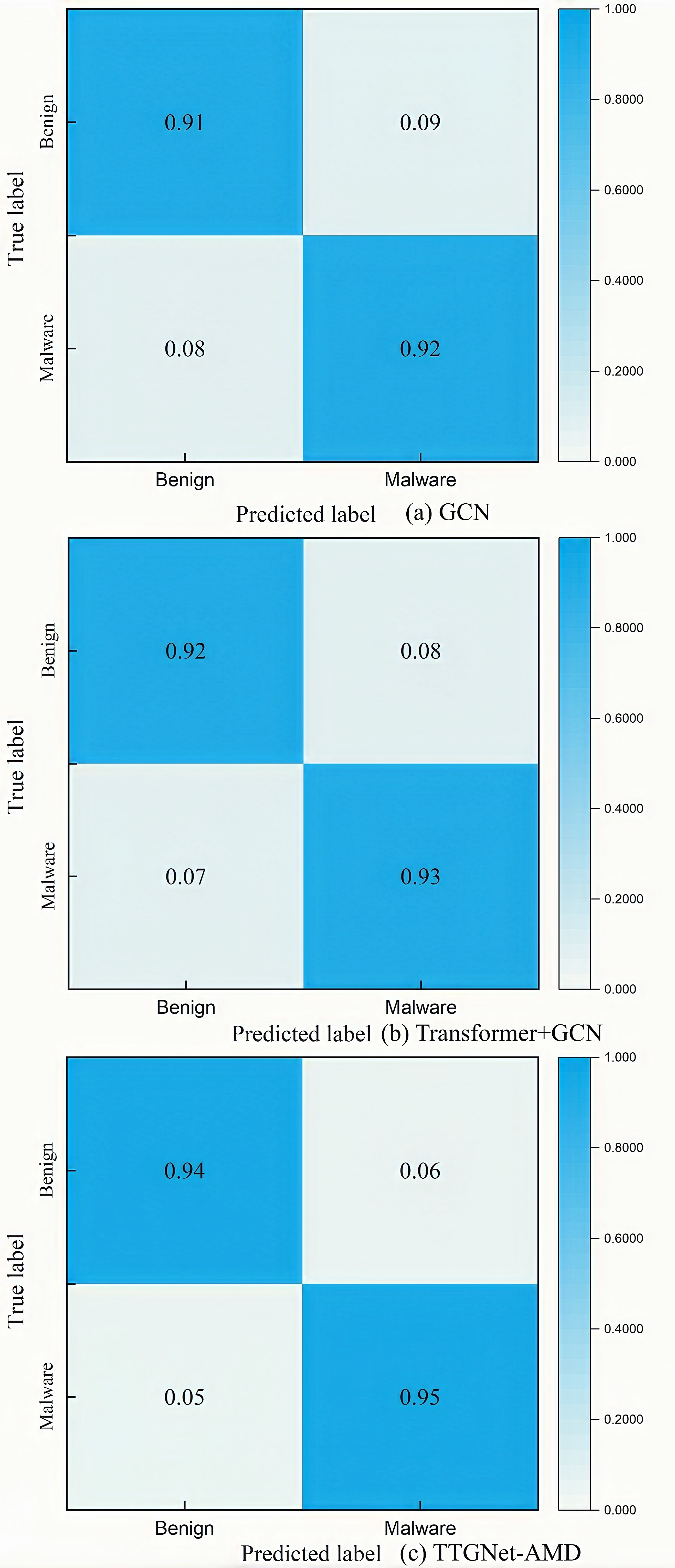
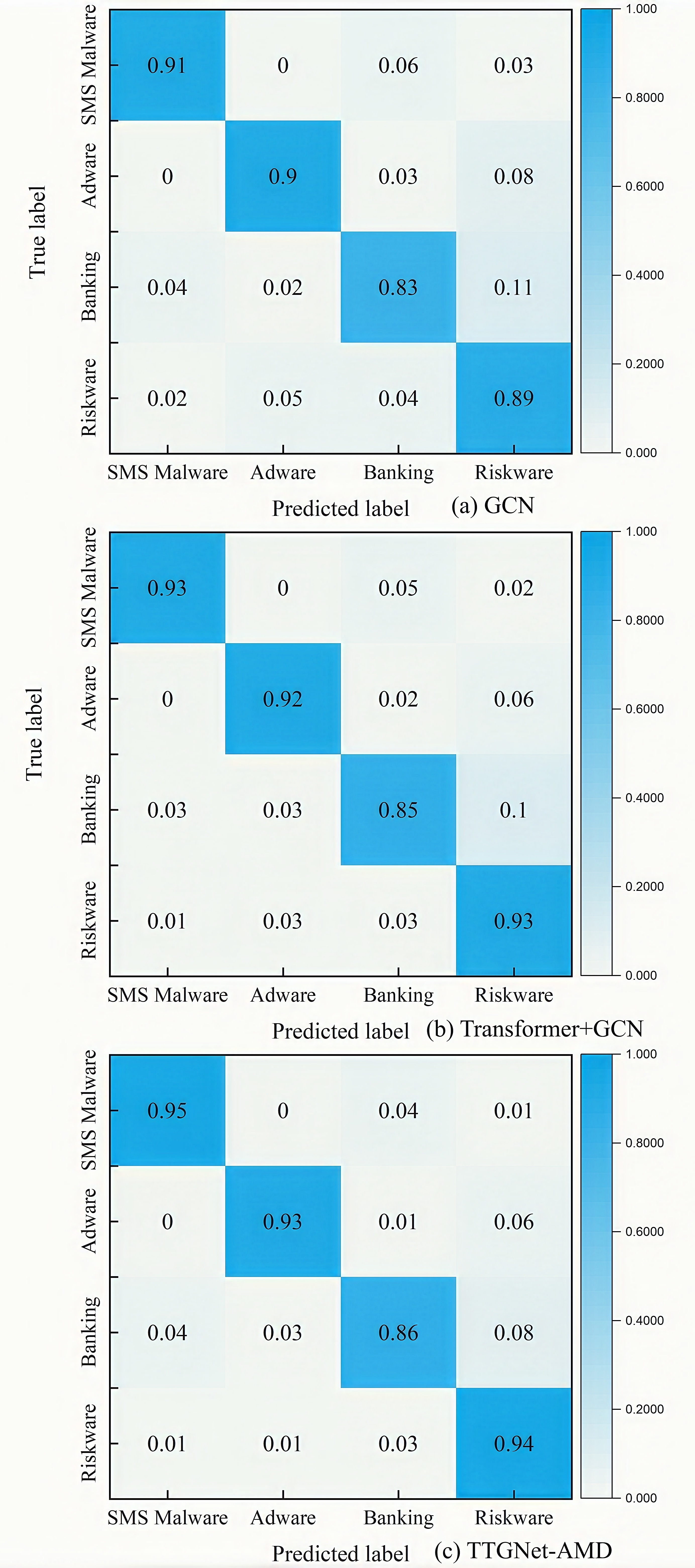
The confusion matrix results of the three models for malware detection on the CICMalDroid2020 and the Drebin dataset are shown in Figs. S8 and S9. The confusion matrix results of the three models for malware category classification on the CICMalDroid2020 dataset are shown in Fig. S10.
The experimental results confirm that by integrating the structural feature extraction capability of the graph convolutional network (GCN), the global dependency modeling advantage of the Transformer, and the temporal feature learning mechanism of the long short-term memory network (LSTM), the TTGNet-AMD method achieves collaborative optimization of multimodal features and can more accurately distinguish between easily confused malware categories.
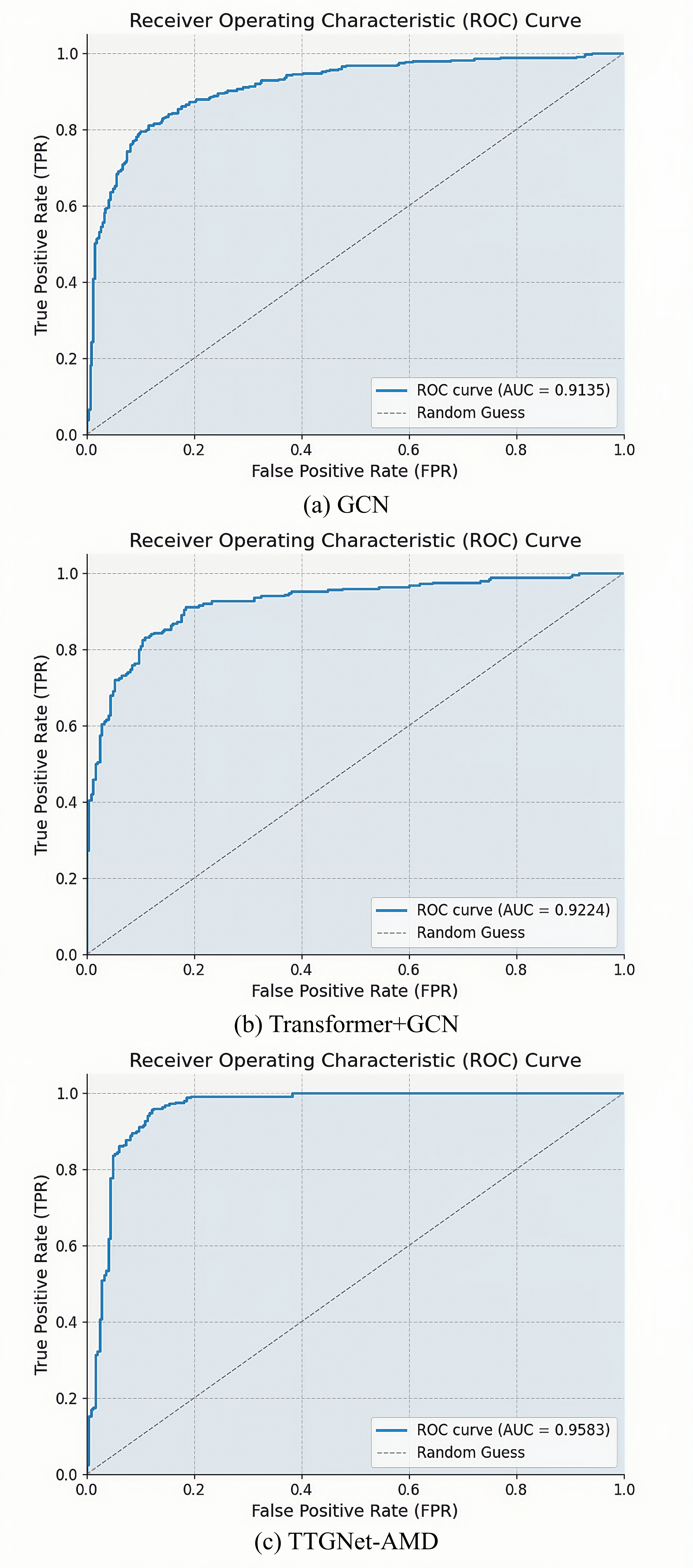
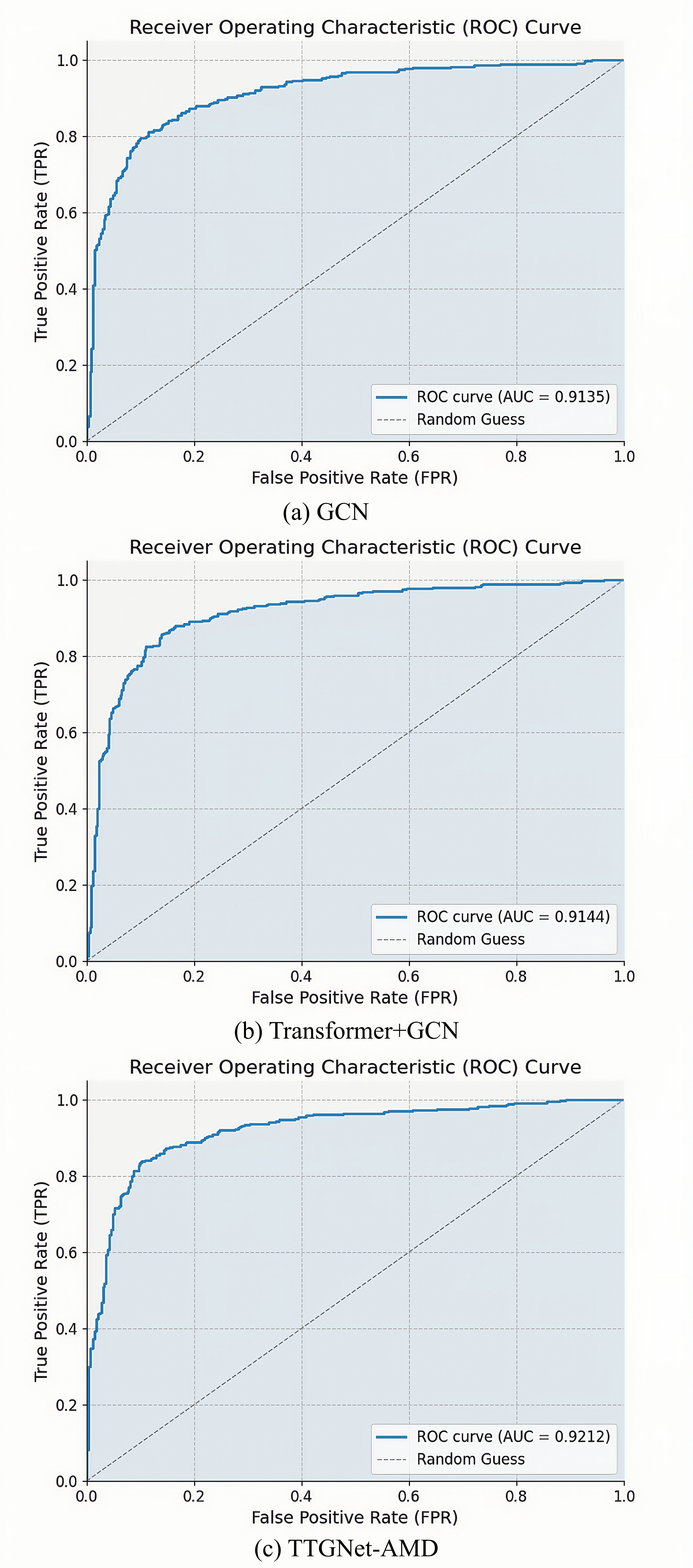
In malware detection experiments, the area under the curve (AUC) curve is used as an evaluation indicator to measure the classification performance of malware detection models. Especially in binary classification problems, it is based on the area under the receiver operating characteristic curve (ROC) and can provide a comprehensive evaluation of the overall performance of the model. The closer the AUC value is to 1, the better the classification performance of the model. The Fig. S11 shows the ROC curves and AUC values of the three models for malware detection on the CICMalDroid2020 dataset. The ROC curves of the three models for malware detection on the Drebin dataset are shown in Fig. S12.
The experimental results show that the AUC value of the GCN model based on a single feature achieves approximately 91% on both the CICMalDroid2020 and Drebin datasets. After incorporating the Transformer module, the AUC value of the model increases by roughly 1%. In contrast, the complete TTGNet-AMD method, which integrates multimodal features, attains AUC values of 95.83% and 95.60% on the respective datasets, representing an improvement of 4.1 to 4.5 percentage points over the GCN model based on a single feature. These findings confirm that our proposed TTGNet-AMD method, through the fusion of multimodal features, exhibits superior malware detection capabilities across different datasets compared to models relying solely on a single feature, thereby validating the efficacy of the multimodal fusion strategy.
Comparison with other deep learning models and methods
In this section, the proposed TTGNet-AMD method is systematically compared with several graph neural network models and alternative research approaches on the CICMalDroid2020 and Drebin datasets. The graph neural network models under comparison include GCN, graph attention network (GAT), and Graph Sample and AggreGatE (GraphSAGE). Other research methods encompass the ANFIS model (Atacak, Kılıç & Doğru, 2022) and the Atacak approach (Atacak, Kılıç & Doğru, 2022). Through comprehensive experimental comparisons and rigorous analysis, the superiority of the proposed TTGNet-AMD method over other graph neural network models and competing methods is demonstrated. All the aforementioned methods were employed to perform malware detection experiments on the CICMalDroid2020 and the Drebin dataset. The detailed performance comparison results are presented in Tables 2 and 3.
| Algorithm | Evaluation indicators | ||||
|---|---|---|---|---|---|
| Accuracy (%) | Precision (%) | Recall (%) | F1-score (%) | TPR (%) | |
| GCN | 91.55 | 91.19 | 90.00 | 90.34 | 90.00 |
| GAT | 91.29 | 91.18 | 90.00 | 90.33 | 90.00 |
| GraphSAGE | 91.35 | 91.29 | 90.00 | 90.14 | 90.00 |
| ANFIS (Atacak, Kılıç & Doğru, 2022) | 93.33 | 94.09 | 93.33 | 93.26 | 93.33 |
| Atacak (Atacak, Kılıç & Doğru, 2022) | 94.67 | 94.78 | 94.67 | 94.66 | 94.67 |
| TTGNet-AMD | 96.30 | 95.76 | 94.33 | 94.27 | 94.33 |
| Algorithm | Evaluation indicators | ||||
|---|---|---|---|---|---|
| Accuracy (%) | Precision (%) | Recall (%) | F1-score (%) | TPR (%) | |
| GCN | 91.43 | 91.35 | 90.00 | 89.69 | 90.00 |
| GAT | 91.10 | 91.05 | 89.27 | 89.42 | 89.27 |
| GraphSAGE | 91.21 | 91.05 | 89.13 | 89.31 | 89.13 |
| ANFIS (Atacak, Kılıç & Doğru, 2022) | 90.00 | 90.98 | 90.67 | 90.68 | 90.67 |
| Atacak (Atacak, Kılıç & Doğru, 2022) | 92.00 | 92.15 | 92.00 | 92.01 | 92.00 |
| TTGNet-AMD | 96.13 | 95.20 | 94.12 | 93.85 | 94.12 |
As can be seen from Table 2, the accuracy of the GCN model in malware detection on the CICMalDroid2020 dataset is 91.55%, the precision is 91.19%, and the recall and F1-score are both above 90%; the accuracy of the GAT model in malware detection is 91.29%, the precision is 91.18%, and the recall and F1-scores are around 90%; the results of the GraphSAGE model in malware detection are close to the results of the above two models, and the evaluation indicators such as accuracy, precision, recall and F1-score are all above 90%. The accuracy and F1-score of the ANFIS method in malware detection are all around 94%. The detection accuracy and recall of the Atacak method (Atacak, Kılıç & Doğru, 2022) are 94.67%, the precision is 94.78%, and the F1-score is 94.66%. Our proposed TTGNet-AMD method has an accuracy of 96.30%, a precision of 95.76%, a recall of 94.33%, and an F1-score of 94.27%. In general, the proposed TTGNet-AMD method performs better than other deep learning models and methods in malware detection.
The Table 3 shows that the accuracy of malware detection by the GCN model is 91.43%, the precision is 91.35%, the recall is 90.00%, and the F1-score is 89.69%; the accuracy and precision of the GAT model are 91.10% and 91.05%, respectively, and the recall and F1-score are 89.27% and 89.42%, respectively; the accuracy, precision, recall and F1-score of the GraphSAGE model are all around 90%. The detection results of various evaluation indicators of the ANFIS method are all above 90%. Our TTGNet-AMD method has an accuracy of 96.13%, a precision of 95.20%, a recall of 94.12%, and an F1-score of 93.85%. In summary, the proposed TTGNet-AMD method performs slightly better than other graph neural network models and methods in malware detection.
Conclusion and future work
This article proposes a multi-modal feature fusion-based Android malware detection method, TTGNet-AMD. This method adopts multiple feature fusion strategies. First, the Apktool tool is utilized to decompile the APK file to extract the features of the opcode sequence, while the Flowdroid tool is leveraged to decompile the APK file to obtain the features of the function call graph. Subsequently, the two types of features will be optimized, and the processed features will be input into the proposed TTGNet model for malware detection and malware category classification. The opcode sequence captures the low-level statistical semantic patterns of the program, while the function call graph reveals its high-level functional structure and the logical relationships between program modules. The complementarity of these two features describes a more comprehensive software behavior, thereby improving the detection accuracy. The experimental results show that the accuracy rate of the TTGNet-AMD method in the malware detection task is 96.30%, and the F1-score is 94.27%. The accuracy rate in the category classification task was 95.12%, and the F1-score was 93.26%.
Although the TTGNet-AMD method has achieved promising results in Android malware detection, there remain areas for further enhancement. In the future, improvements will be made in the following two aspects. First, the current method relies on static analysis techniques and does not encompass the dynamic behavioral features of software during runtime. In the future, dynamic features could be integrated to construct a feature representation that combines both static and dynamic analyses, thereby enhancing the comprehensiveness and accuracy of detection. Second, more extensive and up-to-date experimental datasets will be collected to ensure that the datasets used in experiments are more representative, further strengthening the generalization capability and practical applicability of the model. These improvement directions will contribute to advancing Android malware detection technology toward greater efficiency and accuracy.