
Gunner: playing FPS game Doom with scalable deep reinforcement learning
- Published
- Accepted
- Received
- Academic Editor
- José Santos
- Subject Areas
- Agents and Multi-Agent Systems, Artificial Intelligence, Computer Vision, Data Mining and Machine Learning
- Keywords
- Deep reinforcement learning, Game AI, FPS game, VizDoom
- Copyright
- © 2025 Sun and Zhang
- Licence
- This is an open access article distributed under the terms of the Creative Commons Attribution License, which permits unrestricted use, distribution, reproduction and adaptation in any medium and for any purpose provided that it is properly attributed. For attribution, the original author(s), title, publication source (PeerJ Computer Science) and either DOI or URL of the article must be cited.
- Cite this article
- 2025. Gunner: playing FPS game Doom with scalable deep reinforcement learning. PeerJ Computer Science 11:e3410 https://doi.org/10.7717/peerj-cs.3410
Abstract
Since the introduction of the Deep Q-Network (DQN) algorithm, the reinforcement learning research community has advanced rapidly. Much of the research has focused on the Atari 2600, which uses 2D environments to simulate aspects of the real world. However, 3D game environments are more advantageous in this regard, as they more closely approximate real-world settings. In this work, we focus on training an agent to play the deathmatch scenario in the 3D first-person shooter (FPS) game Doom. A key challenge lies in accurately identifying objects and retaining their spatial positions. We have developed a new agent, named Gunner, trained with a deep reinforcement learning algorithm that incorporates Residual and Long Short-Term Memory (LSTM) blocks for object recognition and memory. In addition, we further enhance the performance of Gunner by integrating Dueling Networks and Noisy Networks. During training, we adopted the AdamW optimizer as the default configuration. All training and testing experiments were conducted on the VizDoom platform. We evaluated the effectiveness of the algorithm components in the deathmatch scenario and further validated the generalization ability of the algorithm in two additional scenarios: “Health Gathering Supreme” and “Defend the Center”. Our experimental results demonstrate that Gunner outperforms several other reinforcement learning algorithms in the FPS game Doom.
Introduction
Since the introduction of the Deep Q-Network (DQN) algorithm (Mnih et al., 2013, 2015), the use of neural networks as function approximators has become a mainstream approach in the field of reinforcement learning (RL). The number of research articles on deep reinforcement learning (DRL) has increased dramatically (Henderson et al., 2018). The original DQN architecture typically consists of two or three convolutional layers followed by a fully connected layer. It processes raw game screen inputs (in the form of pixels) through the convolutional layers and then outputs the action policy via the fully connected layer. Since then, many methods have been proposed to improve the performance of DQN, including Double Q-learning (Van Hasselt, Guez & Silver, 2016), Prioritized Replay (Schaul et al., 2015), Dueling Networks (Wang et al., 2016), Multi-step Learning (Sutton & Barto, 2018), Distributional RL (Bellemare, Dabney & Munos, 2017), Noisy Networks (Fortunato et al., 2018), and their integrated form, Rainbow (Hessel et al., 2018). However, both DQN and its extension Rainbow have been limited to 2D environments, particularly the Atari 2600 games.
Although 2D environments like Atari provide a useful testbed, they lack several critical aspects of real-world applications, including depth perception, spatial reasoning, and the partial observability inherent in dynamic 3D environments. Therefore, transferring DRL methods to more complex and realistic 3D environments is a crucial step toward deploying intelligent agents in domains such as robotics, autonomous driving, and simulation-based training systems.
Recent advances in deep reinforcement learning have shown that improvements in architecture and auxiliary techniques can significantly enhance agent performance, particularly in 2D environments such as the Atari 2600. The IMPALA algorithm (Espeholt et al., 2018), proposed by Espeholt et al. (2018) replaces the conventional three-layer convolutional network with a deeper 15-layer Residual Network (ResNet) (He et al., 2016). This deeper network has been empirically shown to improve agent performance with larger amounts of training data (Schmidt & Schmied, 2021; Agarwal et al., 2022).
The Implicit Quantile Network (IQN) (Dabney et al., 2018) extends distributional RL by learning the full quantile function. By combining quantile regression with deep RL, it approximates the entire return distribution. To improve data efficiency, Data-regularized Q-learning (DrQ) (Kostrikov, Yarats & Fergus, 2020), introduced by Kostrikov, Yarats & Fergus (2020) integrates data augmentation into the RL training pipeline, thereby enhancing generalization when training with limited samples.
For improved representation learning, SPR (Self-Predictive Representations) (Schwarzer et al., 2020), proposed by Schwarzer et al. (2020) introduces a self-supervised temporal consistency loss in combination with data augmentation. Subsequently, the SR-SPR (D’Oro et al., 2022) variant incorporates periodic network resets to stabilize learning and improve long-term performance. The BFS algorithm (Schwarzer et al., 2023) advances the state of the art by adopting a deeper ResNet encoder and increasing the replay ratio, achieving superior performance on Atari benchmarks.
Most of the aforementioned algorithms fall under model-free RL, which learns optimal policies or value functions directly from experience. In contrast, model-based RL has shown particular effectiveness in games that require long-term planning, such as Go and Chess. A landmark example is provided by AlphaGo (Silver et al., 2016), which combined Monte Carlo Tree Search (MCTS) (Coulom, 2006) with deep RL to defeat world champion Lee Sedol. Its successor, AlphaGo Zero (Silver et al., 2017), dispensed with human data and trained entirely via MCTS-based self-play, achieving a 100–0 record against the original system. AlphaZero (Silver et al., 2018) generalized this approach to Chess and Shogi, while MuZero (Schrittwieser et al., 2020) unified model-based planning with model-free learning, achieving state-of-the-art results across domains, including Atari games.
In games that require long-term planning and accurate lookahead, search has proven to be an effective approach. However, most model-based RL algorithms have significant limitations. Their designs are often tailored to specific environments, making them difficult to adapt to other settings. Moreover, recent work has shown that model-free RL algorithms have achieved superhuman performance in large-scale real-time strategy games, such as Dota 2 (Berner et al., 2019) and StarCraft II (Vinyals et al., 2019).
However, most of these algorithms were developed and evaluated primarily in 2D settings. These environments provide full observability, relatively simple dynamics, and low-dimensional visual inputs, rendering them far less challenging than real-world problems. In contrast, 3D environments involve higher-dimensional observations, perspective distortion, occlusion, and more complex physics-based interactions. These factors make representation learning and credit assignment substantially more challenging in 3D RL.
Several recent studies have begun addressing these challenges. Jaderberg et al. (2019) employed multi-agent RL to achieve human-level performance in the “Capture the Flag” mode of the 3D multiplayer game Quake III Arena. Zieliński & Markowska-Kaczmar (2021) applied visual-input-based DRL models to robot navigation in 3D environments. Singh et al. (2021) innovatively proposed the Structured World Belief (SWB) model to address observability challenges, demonstrating its effectiveness in enhancing RL performance. Ge et al. (2024) adapted the Decision Transformer (DT) (Chen et al., 2021) to 3D navigation tasks, reporting both the strengths and stability limitations of DT variants in handling partial observability and continuous control. Kang et al. (2023) introduced Graph-based Memory Reconstruction (GBMR), improving sample efficiency and accelerating learning on Atari games compared to traditional RL methods. Khan, Muhammad & Naeem (2025) investigated the performance of PPO in the Deadly Corridor scenario of the 3D game Doom, providing insights for optimizing RL agents in this environment.
These works reflect both algorithmic and environmental advances that help bridge the gap between 2D and 3D reinforcement learning. Despite their success, both model-free and model-based approaches have rarely been thoroughly explored in visually rich, partially observable 3D tasks. Our work aims to bridge this gap by adapting and extending model-free DRL techniques to extend their applicability to these 3D environments, with a focus on the Doom environment.
In this article, we propose a model-free RL algorithm, the Gunner algorithm, and use it to train an agent to play the deathmatch scenario in the well-known first-person shooter (FPS) game Doom. Compared with Atari 2600 games, the characteristics of Doom’s 3D environment are more closely aligned with real-world problems. We use the VizDoom (Kempka et al., 2016) platform as the platform for training and evaluating agent performance in Doom. This setting provides a high-dimensional, partially observable, and fast-paced testbed for advancing 3D reinforcement learning. Our experiments show that the Gunner agent outperforms the game’s built-in AI as well as several classic DRL algorithms. Finally, we analyze the contributions of different components and techniques of the proposed algorithm and outline directions for future research.
Materials and Methods
Reinforcement learning
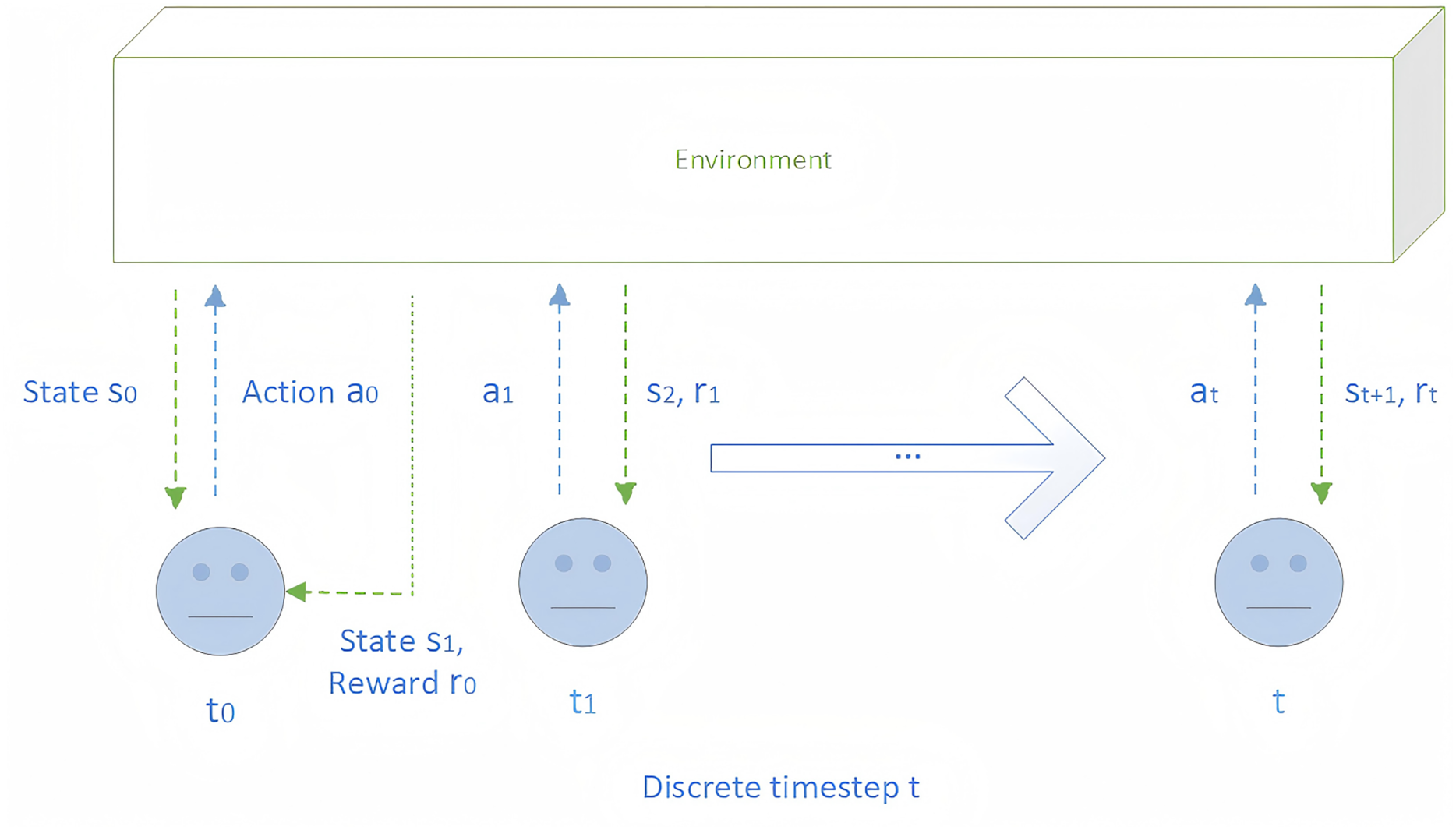
The goal of RL is to enable an agent to learn an optimal policy π* in an uncertain environment, maximizing the expected cumulative discounted reward. In practice, the RL problem is usually formalized as a Markov Decision Process (MDP) (Puterman, 2014). In most RL scenarios, at each discrete time step t, the agent receives a state st ∈ S from the environment and selects an action at ∈ A according to a policy π. The environment then returns the next state st+1 along with a reward rt ∈ R. Therefore, the process shown in Fig. 1 can be formalized as a tuple <S, A, P, R, γ>, where S denotes the set of states; A, the set of available actions; P: S * A → (S), the state transition function with (S) representing the probability distribution over states; R, the set of rewards provided by the environment; and γ ∈ [0, 1), the discount factor that prioritizes immediate rewards over delayed ones.
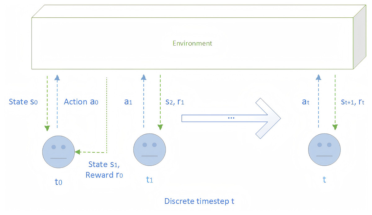
Figure 1: The interaction process between agent and environment.
In RL, two value functions play a crucial role: the state-value function and the action-value function. To derive these two functions, we first need to define the expected cumulative discounted reward Ut at a discrete time step t:
(1) Based on the expected cumulative discounted reward Ut at a discrete time step t, we can derive the action-value function Qπ corresponding to policy π:
(2) Then, by taking the expectation over actions according to policy π, we derive the state-value function Vπ:
(3) In this article, we focus primarily on the action-value function Q. Our goal is to enable the agent to learn an optimal policy π* through interaction with the environment. As shown in Eq. (2), the optimal action-value function Q* is defined by the Bellman recurrence:
(4) A common approach to learning the optimal action-value function Q* is the Temporal-Difference (TD) learning algorithm, which approximates Q* by minimizing the temporal-difference (TD) error:
(5) where is commonly referred to as the temporal-difference (TD) target.
Deep Q-Network
The Deep Q-Network (DQN) algorithm was originally proposed by Mnih et al. (2013), Mnih et al. (2015). In reinforcement learning, the objective is to maximize the expected cumulative discounted reward associated with taking an action a, which is represented by the action-value function Qπ(s, a) under policy π. The optimal action-value function Q*(s, a) is defined as:
(6) which corresponds to the maximum achievable value of Qπ(s, a) over all possible policies.
In practice, the action-value function Qπ(s, a) is typically approximated using a function approximator. In DQN, a neural network parameterized by θ is employed to approximate Qπ(s, a). The original DQN architecture consists of three convolutional layers followed by two fully connected layers, and its parameters θ are updated using the TD learning algorithm. We need to maximize Qπ(s, a) as much as possible, preferably to the Q*(s, a). The ultimate objective is to approximate the optimal action-value function as closely as possible, i.e., to train the network such that Qθ(s, a) ≈ Q* (s, a).
In practice, the parameters θ are updated via gradient descent using the TD learning algorithm. Within TD learning, two key quantities are defined: the TD target and the TD error. When the agent observes a state st and selects an action at, the environment returns a reward rt and a subsequent state st+1. The TD target can then be computed as:
(7)
At time step t, the expected cumulative discounted reward estimated by DQN is given by:
(8) Since the reward rt is directly obtained from the environment, the TD target yt provides a more accurate estimate. The TD error δt is then defined as the difference between the TD target yt and the current estimate qt:
(9) The objective is to minimize the TD error δt, i.e., to bring the current estimate qt closer to the TD target yt. This is achieved by updating the network parameters θ via gradient descent. Accordingly, the loss function is defined as:
(10)
Unlike some on-policy RL algorithms such as A3C (Mnih et al., 2016) and PPO (Schulman et al., 2017), DQN is an off-policy algorithm. In DQN, the agent generates trajectories using one policy while learning a separate target policy from these trajectories. In practice, this is implemented using experience replay. At each time step t, the trajectory (st, at, rt, st+1) is stored in a replay buffer, and the agent randomly samples mini-batches from the buffer to update Qθ. The ε-greedy strategy is typically employed in conjunction with experience replay: at each time step t, the agent selects the action with the highest Q-value according to the network with probability 1-ε, and a random action with probability ε.
The agent trained using DQN achieved near-human-level performance on Atari 2600 games. Many subsequent value-based RL algorithms build upon this architecture, the most notable of which is Rainbow, proposed by Hessel et al. (2018). As an enhanced version of DQN, Rainbow incorporates six key improvements: Double Q-learning (Van Hasselt, Guez & Silver, 2016), Prioritized replay (Schaul et al., 2015), Dueling networks (Wang et al., 2016), Multi-step learning (Sutton & Barto, 2018), Distributional RL (Bellemare, Dabney & Munos, 2017), and Noisy networks (Fortunato et al., 2018). Each of these components improves performance individually. Since they address distinct limitations of DQN and can be integrated within a single framework, Rainbow significantly outperforms DQN. Agents trained with Rainbow surpassed human performance in 40 out of 57 Atari 2600 games, achieving state-of-the-art results.
DRQN
To address the problem of partially observable environments, Hausknecht & Stone (2015) proposed replacing the first fully connected layer of DQN with a recurrent layer, typically a long short-term memory (LSTM). This results in the Deep Recurrent Q-Network (DRQN) algorithm. The key advantage of DRQN over DQN is its ability to retain information over time. In 2D game environments, such as Atari 2600, the screen pixel information largely captures the environment state; thus, strong memory capabilities are generally unnecessary for the agent to infer the state and determine the appropriate sequence of actions. However, in the 3D FPS game Doom, the agent observes only a partial view of the environment, making memory-capable algorithms crucial. In deep RL literature, LSTM units are predominantly employed as the memory component, as seen in A3C (Mnih et al., 2016), DRQN (Hausknecht & Stone, 2015), Recurrent Replay Distributed DQN (Kapturowski et al., 2018), and IMPALA (Espeholt et al., 2018).
In DRQN, the action-value function is computed as Qθ(ot, ht−1, at), in contrast to Qθ(st at) in DQN. Here, ot represents the observation at time step t, and ht−1 denotes the hidden state from the previous time step, propagated through the recurrent network. Using an LSTM as the memory unit, the hidden state is updated as ht = LSTM(ht−1, ot), and the action-value function at time step t is then computed as Qθ(ht, at).
ResNet
ResNet, or Residual Networks, was introduced by He et al. (2016) as a breakthrough architecture in deep learning, which was designed to address the challenges associated with training very deep neural networks. In traditional deep networks, gradients can become too small to effectively update early-layer weights as network depth increases, leading to performance degradation. To overcome this issue, ResNet incorporates skip connections (or residual connections), which allow the input from an earlier layer to bypass one or more intermediate layers and be directly added to a later layer. This simple yet powerful design enables the training of networks with hundreds or even thousands of layers, significantly enhancing the model’s capacity to capture complex patterns and features.
The key component of ResNet is the residual block, which performs the following operation:
(11) Here, x is the input to the residual block, F(x, {Wi}) denotes the function implemented by the convolutional layers with parameters {Wi}, and the skip connection adds the input x directly to the output. This enables the network to preserve essential features from earlier layers while learning new, complex representations in deeper layers.
Dueling networks
Previously, we calculated the optimal action-value function Q*(s, a) in DQN. To compute the optimal advantage function A*(s, a) in Dueling Networks, the optimal state-value function V*(s) must also be determined. As derived in the reinforcement learning section, the state-value function under policy π is Vπ(s). Analogous to the derivation of Q * (s, a), the optimal state-value function is given by:
(12) V*(s) denotes the maximum expected cumulative discounted reward obtainable from state s.
The optimal advantage function is defined as:
(13) Then the optimal action-value function can then be expressed as:
(14) To address the non-identifiability problem, it is common to subtract the maximum advantage across actions:
(15) In practice, taking the mean of A*(s, a) across actions has been found to yield better performance. Following this derivation, the action-value function in Dueling Networks can be expressed as:
(16) The network parameters are then updated using the TD algorithm, analogous to the DQN training procedure.
Noisy networks
Noisy Networks (NoisyNets) extend conventional neural networks by introducing stochasticity into the weights and biases. Specifically, each weight and bias parameter is perturbed by a learnable noise variable, enabling exploration to be incorporated directly into the function approximator. Unlike fixed randomness, these noise parameters are trainable and updated via gradient descent. A noisy linear layer can be formally defined as:
(17) Here, x denotes the input vector and y the outputs. The weight parameters are reparameterized as μw + σw εw, and the bias parameters as μb + σb εb, where denotes element-wise multiplication. The terms μw, σw, μb, and σb are learnable parameters, while εw and εb are random noise variables. In our network architecture, εw is sampled from a factorised Gaussian distribution as a random matrix, and εb is sampled as a random vector from the same distribution.
We next derive the loss function of the network. Let ς denote the set of learnable noise parameters in the NoisyNet layers. The action-value function, originally parameterized as Q(s,a;θ), can thus be reparameterized as Q(s,a;ς). Since our network architecture is based on DRQN, the action-value function at time step t is expressed as Q(ht,at;ς), where ht denotes the hidden state. Accordingly, the loss function for Gunner is defined as:
(18)
Results
Scenario
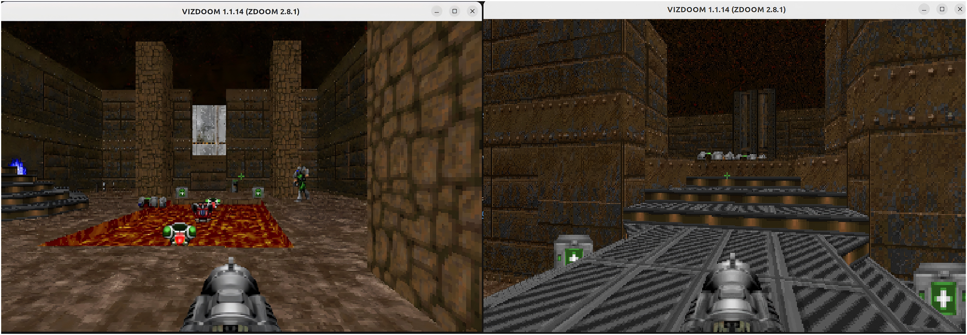
We use the VizDoom platform (Kempka et al., 2016; Wydmuch, Kempka & Jaśkowski, 2018) to train and evaluate our agents in the deathmatch scenario of the Doom game. VizDoom is a lightweight and highly customizable artificial intelligence (AI) research platform developed by Wydmuch, Kempka & Jaśkowski (2018) built on ZDoom—the most widely used modern Doom source port. The platform provides multiple built-in scenarios; among them, the deathmatch scenario involves both item acquisition and enemy elimination, and features the most complex map configuration. The “Deathmatch” scenario is illustrated in Fig. 2.
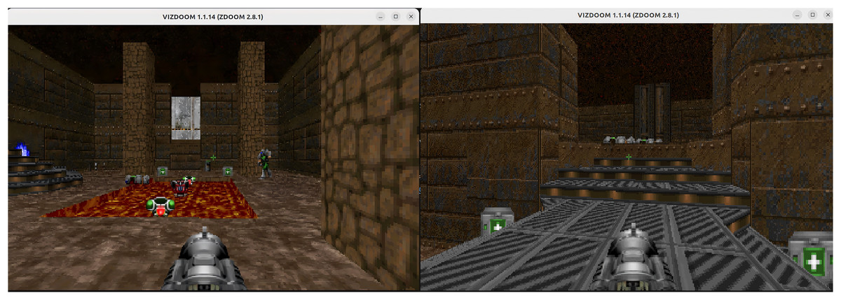
Figure 2: The deathmatch scenario.
In the deathmatch scenario, the agent is spawned at random locations within an arena filled with resources, such as medical kits, armor, and ammunition. Enemies are also randomly spawned in the arena, whose objective is to attack the agent. For our experiments, the scenario is configured with eight enemies. The arena further contains a square magma pool at its center, which decreases the agent’s health upon entry. The agent’s objective is to maximize enemy eliminations while minimizing self-inflicted deaths, since its weapon is a rocket launcher that inflicts area-of-effect damage and often harms the agent itself.
To evaluate the generalization performance of the algorithms in the Doom environment, we additionally conducted experiments on two supplementary scenarios: Health Gathering Supreme and Defend the Center.
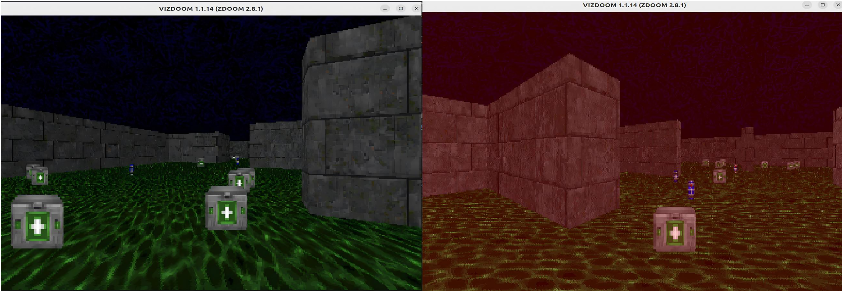
The Health Gathering Supreme scenario features a relatively complex, maze-like map with multiple branching paths. In this environment, the agent continuously loses health over time. To prolong survival, it must collect medical kits scattered throughout the map to restore health. In addition to medical kits, explosive items are also present; picking them up causes further health loss. The agent’s objective in this scenario is to maximize survival time until the episode ends. Successfully achieving this objective requires the agent to possess spatial memory of the environment, which motivates its selection for our experiments. The Health Gathering Supreme scenario is illustrated in Fig. 3.
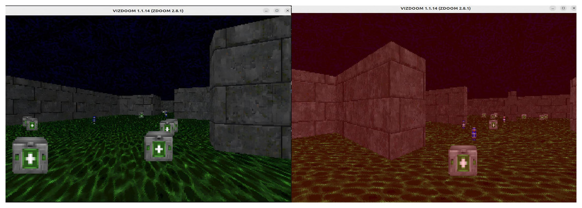
Figure 3: The Health Gathering Supreme scenario.
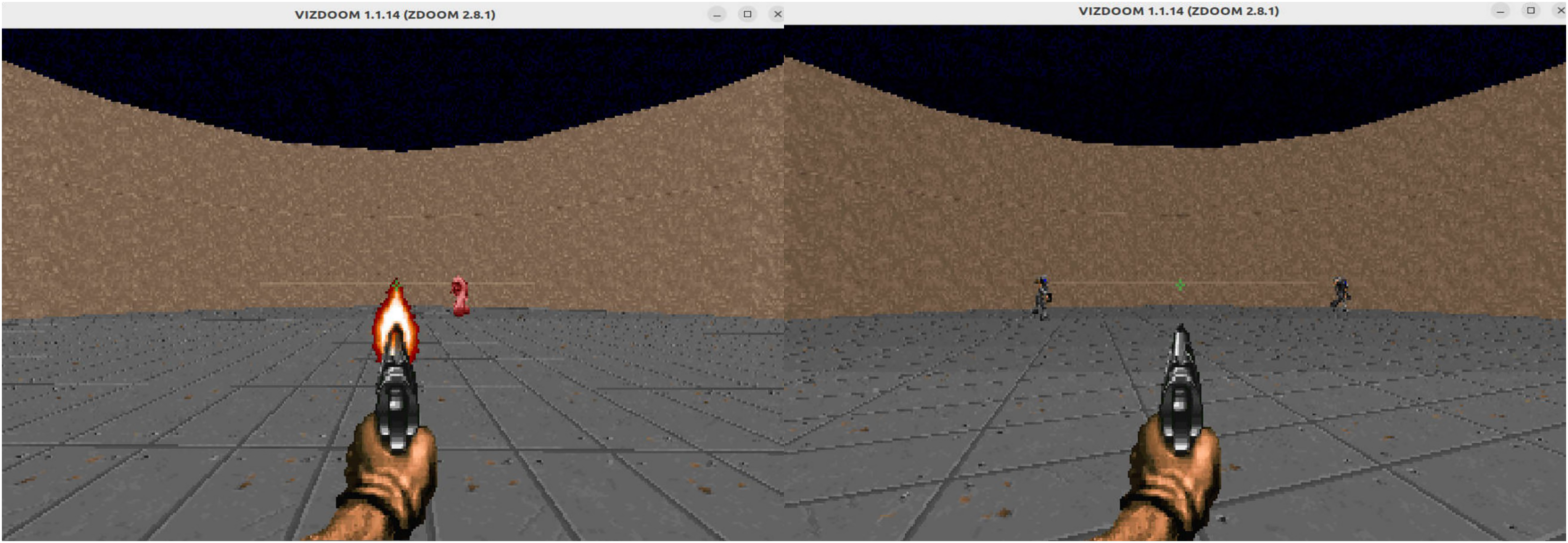
The Defend the Center scenario features a relatively simple map layout but places higher demands on the agent’s target recognition and attack capabilities. The map consists of a circular arena in which the agent is fixed at the center and can only rotate its perspective. Five melee enemies spawn along the circular boundary; each can be eliminated with a single shot but respawns after a short delay. Because the agent has limited ammunition, being defeated by the melee enemies is ultimately unavoidable, and the episode ends once the agent is killed. The Defend the Center scenario is illustrated in Fig. 4.
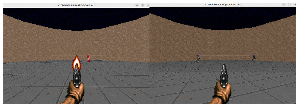
Figure 4: The Defend the Center scenario.
Model
This study is guided by two central research questions: (1) Does employing a larger ResNet architecture, rather than a traditional Convolutional Neural Network (CNN), enhance agent performance in Doom? and (2) Is the LSTM unit currently the most effective memory mechanism in reinforcement learning? To address these questions, we analyze the performance of our proposed agent, Gunner, in the Doom deathmatch scenario, with detailed results presented in the analysis section. Before discussing these findings, we first describe the model architecture and training components of Gunner.
Basic model
Gunner builds upon the model proposed by Lample & Chaplot (2017), while retaining several advantageous techniques from the original design, including action binding, reward shaping, frame skipping, and the game features network. (1) Action binding: Experimental results indicate that shooting while moving left or right is ineffective, as the crosshair cannot be aligned with the enemy. Therefore, we decoupled the shoot action from lateral movement, reducing the action space from 53 to 35 possible action combinations. (2) Reward shaping: The reward parameter settings (see Table 1) largely follow the original design. Eliminating enemies and collecting items yield positive rewards, whereas shooting, taking damage, dying, or committing suicide incur negative rewards. Additionally, the agent receives a small continuous reward proportional to its movement distance, which was found to encourage exploration of the environment. (3) Frame skipping: The number of skipped frames between steps is set to three, instead of four as recommended in the baseline model. This adjustment proved more effective in handling complex scenarios such as deathmatch.
| Parameters | Agent behavior | Rewards |
|---|---|---|
| DISTANCE | Move distance | +9e−5 |
| KILL | Kill an enemy | +10 |
| DEATH | Dead | −10 |
| SUICIDE | Commit suicide | −12 |
| MEDIKIT/ARMOR | Pick up a health kit or armor | +0.4 |
| WEAPON/AMMO | Pick up a weapon or bullet | +0.5 |
| INJURED | Lose blood volume | −0.5 |
| USE_AMMO | Shoot | −0.2 |
Scalable network
In computer vision, the ResNet architecture proposed by He et al. (2016) has been widely adopted. By incorporating skip connections, ResNet enables the construction of neural networks with hundreds or even thousands of layers, profoundly influencing the development of deep learning. In deep reinforcement learning, many algorithmic models still rely on standard two- or three-layer CNNs, which are relatively shallow given current computational capabilities. This raises the question of whether ResNet can replace the standard three-layer CNN to create a scalable network architecture and thereby enhance agent performance. The IMPALA algorithm, proposed by Espeholt et al. (2018), realizes this concept by replacing the three-layer CNN with a 15-layer ResNet, increasing both network capacity and architectural complexity. In Gunner, we adopt the ResNet architecture from IMPALA for the CNN component and provide an extensible interface to support deeper networks, such as a 30-layer ResNet. Since IMPALA was evaluated in 2D Atari games, the effectiveness of ResNet in a 3D FPS environment like Doom remains to be experimentally verified.
More powerful optimizer
The original DQN employs RMSProp as its default optimizer. In recent years, several DRL algorithms have adopted the Adam optimizer (Kingma & Ba, 2014), achieving superior performance compared to RMSProp. Inspired by the work of Ceron & Castro (2021) and Schwarzer et al. (2023), we adopt the AdamW optimizer (Loshchilov & Hutter, 2018), which decouples weight decay from the gradient update process and addresses certain limitations of the original Adam regarding weight regularization and generalization. In our experiments, we set the weight decay of AdamW to 0.01 and compare the effects of using AdamW vs. RMSProp on the agent’s performance.
Add something improvements
Inspired by Rainbow (Hessel et al., 2018), we further integrate two enhanced network architectures into Gunner: Dueling networks (Wang et al., 2016) and Noisy networks (Fortunato et al., 2018). (1) Dueling networks, proposed by Wang et al. (2016) decompose the action-value function Qθ(s, a) into the state-value function Vθ(s) and the advantage function Aθ(s, a) := Qθ(s, a) – Vθ(s). This decomposition reduces the interference of action selection on state-value estimation, accelerates the learning process, and improves policy stability. (2) Noisy networks, introduced by Fortunato et al. (2018) replace the traditional ε-greedy strategy by adding learnable noise parameters to the linear layers of the output value in DQN, thereby enhancing exploration.
Putting it all together
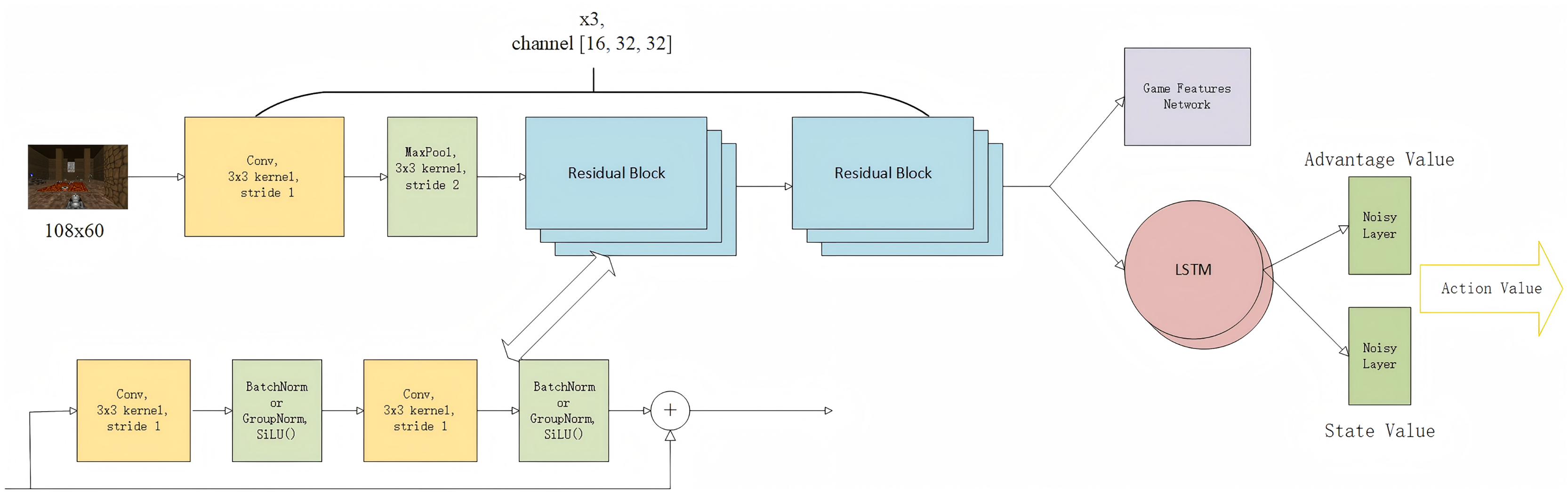
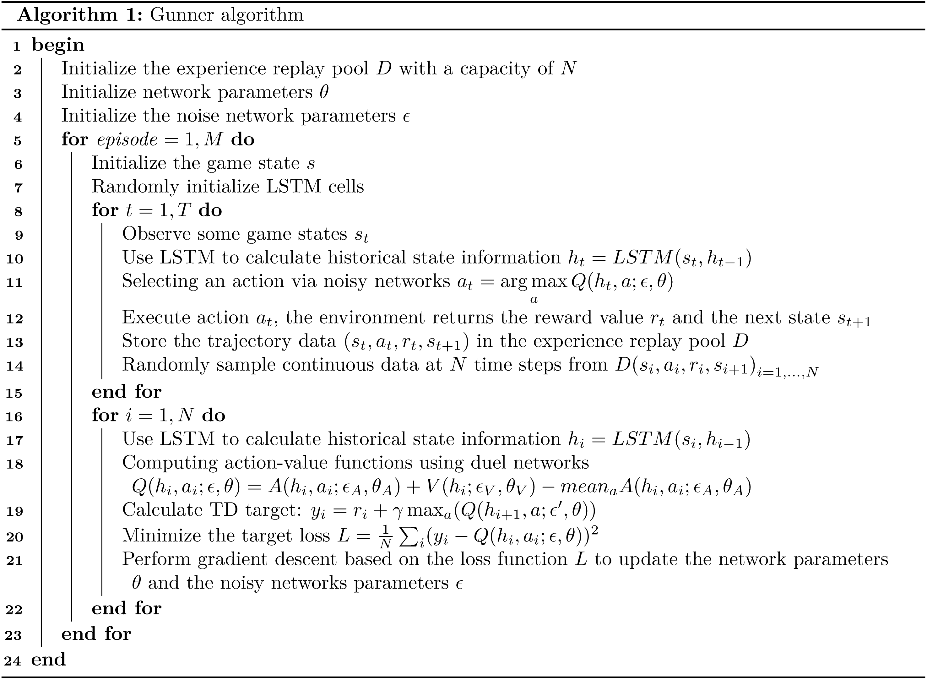
We propose the Gunner algorithm, which integrates multiple advanced techniques into a unified framework. As illustrated in Fig. 5, the architecture comprises four key components: (1) a 15-layer deep convolutional backbone, designed to be scalable and capable of fully exploiting pixel-level information from the game engine; (2) an LSTM unit that serves as the memory module, capturing temporal dependencies and handling partial observability across frames; (3) a game feature detection module, consisting of fully connected layers, which analyzes feedback from the game engine to detect the presence of props or enemies in the current frame, following the approach of Lample & Chaplot (2017); and (4) a decision-making module incorporating Dueling and Noisy Networks, where the LSTM output is used to compute the advantage and state value, which are then combined to form the final action-value estimate. This modular and extensible architecture enables Gunner to adapt effectively to complex visual environments and make informed decisions under uncertainty. The algorithm flowchart is shown in Fig. 6.
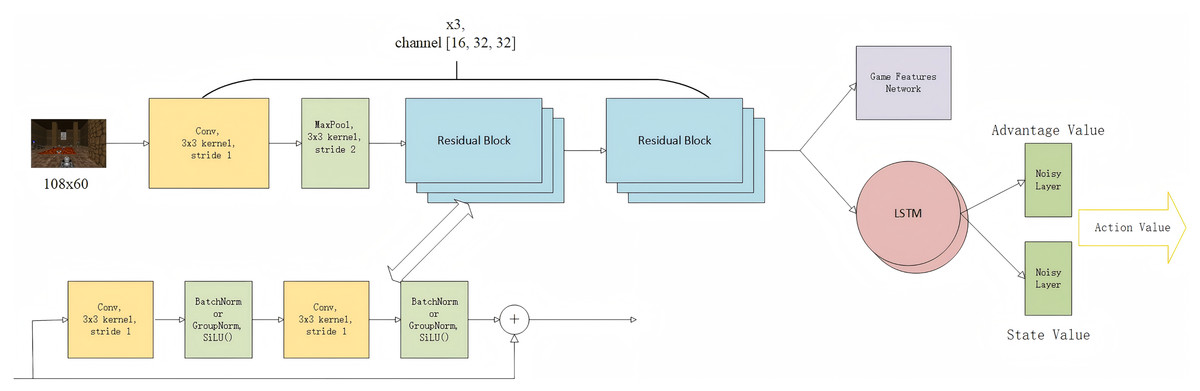
Figure 5: Model architecture.
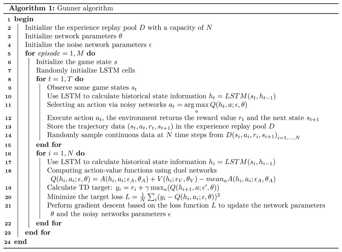
Figure 6: Gunner algorithm flowchart.
Analysis
To evaluate the contributions of individual components within Gunner, we conducted a series of controlled experiments under fixed parameter settings. Training was performed on an Intel Xeon Gold 6122 CPU with an NVIDIA RTX A4000 GPU, while local testing used an AMD Ryzen 7 PRO 5850U CPU with AMD Radeon™ Graphics GPU. All hyperparameters employed during training and testing are summarized in Table 2. Unless otherwise stated, all subsequent experiments utilize the hyperparameter values listed in this table. The following sections present detailed analyses of each component’s impact on agent performance, including the effects of network architecture, memory modules, optimizers, and auxiliary improvements.
| Parameter | Value | Parameter | Value |
|---|---|---|---|
| Batch size | 32 | Learning rate | 0.0002 |
| Dropout | 0.2 | Replay buffer | 1,000,000 |
| γ | 0.99 | Gradient clipping | [−5, 5] |
| Weight decay | 0.01 | NoisyNet init_std | 0.5 |
For experimental evaluation, we employed scenario-specific metrics. (1) Deathmatch scenario: The primary metric is the number of Frags. Frags are chosen to encourage rational strategies, ensuring that the agent maximizes kills while minimizing deaths, particularly suicides, thereby maintaining a favorable kill/death (K/D) ratio. (2) Health Gathering Supreme scenario: The agent’s survival time is measured, including both the maximum survival time within the evaluation interval and the average survival time per episode. (3) Defend the Center scenario: The number of enemies eliminated by the agent is used as the evaluation metric, considering both the maximum number of kills in an evaluation interval and the average kills per episode.
We first evaluated Gunner in the most complex deathmatch scenario, performing comparative experiments to assess the contributions of its individual components and to benchmark its performance against other DRL algorithms.
AdamW optimizer better
Since the choice of optimizer can significantly affect performance, we first conducted a comparative evaluation between the AdamW and RMSProp optimizers. Based on these results, the optimizer demonstrating superior performance was adopted for all subsequent experiments. The comparison results are presented in Fig. 7.
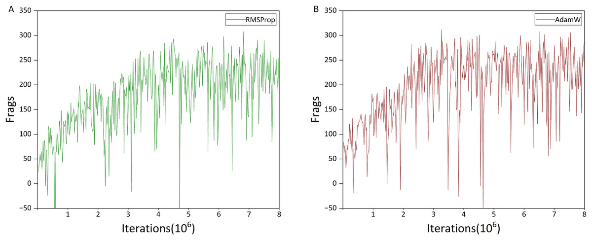
Figure 7: Comparison of the impact of different optimizers.
Figures 7A and 7B show the performance of the agent trained with RMSProp and AdamW optimizers, respectively. To reduce computational cost and training time, we used the Gunner model without Dueling and Noisy Networks for this comparison. The only difference between the two models is the choice of optimizer.
The x-axis of the figure represents training iterations (in millions), while the y-axis represents the Frags value, defined as the number of kills minus the number of suicides. Unless otherwise stated, all subsequent deathmatch training figures use the same axis conventions.
As shown in Fig. 7, the choice of optimizer does not affect the final performance of the agent, which reaches a Frags value close to 310 within eight million iterations. However, the agent trained with AdamW achieves this level in approximately three million iterations, compared to seven million iterations for RMSProp. Additionally, between two and three million iterations, performance improvement with AdamW is more linear, whereas RMSProp exhibits temporary performance drops. These results indicate that AdamW not only accelerates training but also provides more stable learning, and is therefore adopted as the default optimizer in subsequent experiments.
Dueling networks has another function
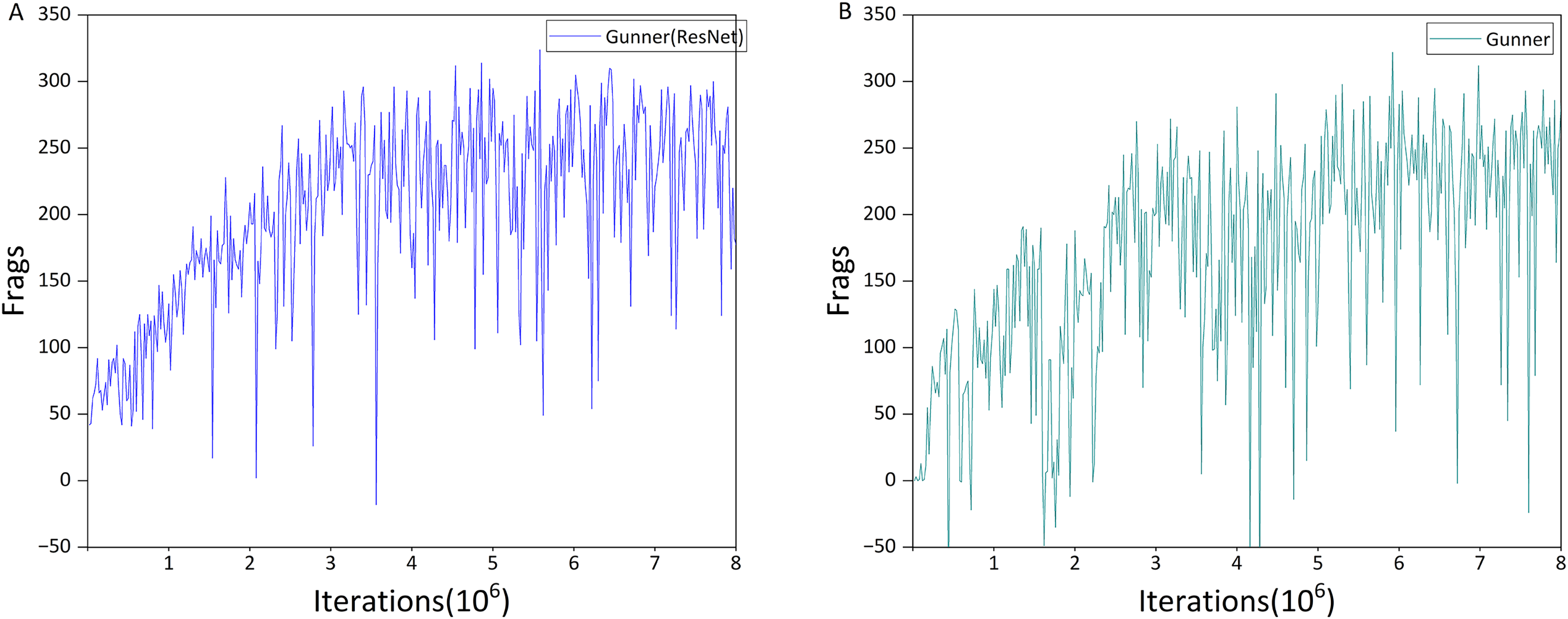
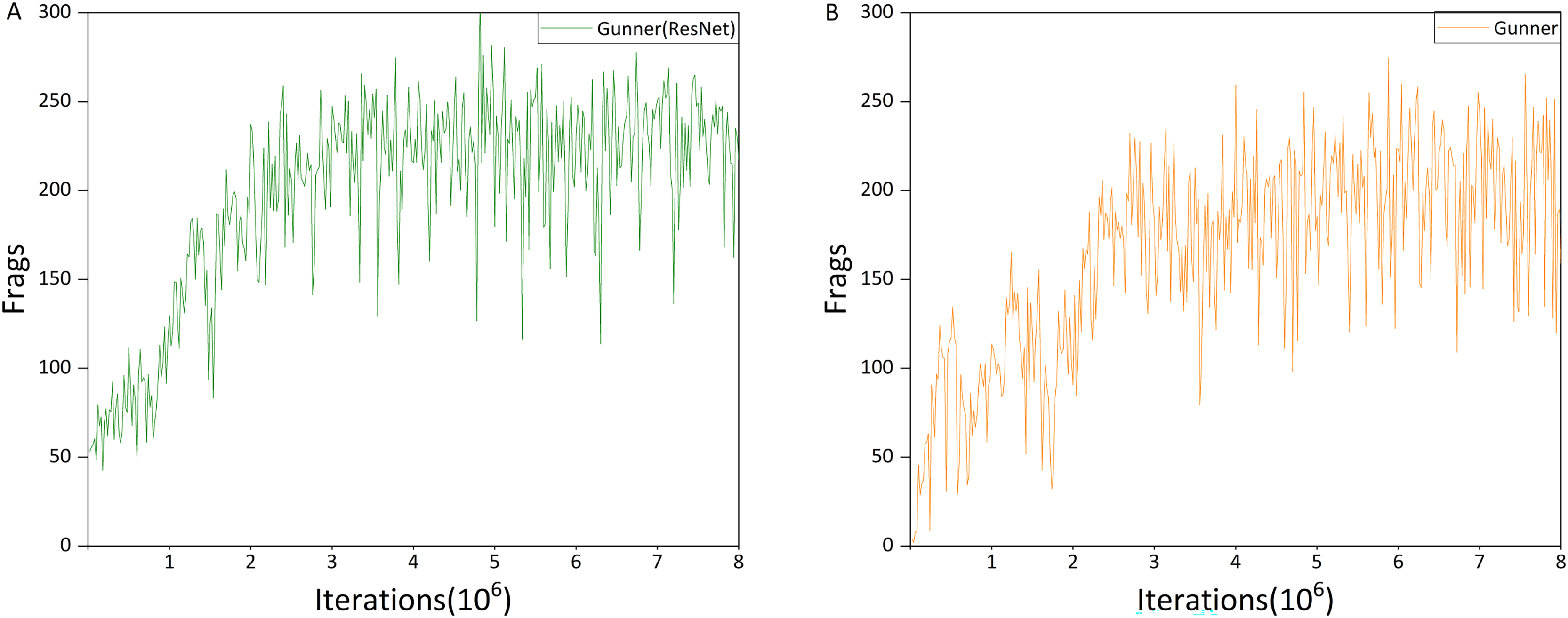
As shown in Figs. 7B and 8A, its direct impact on agent performance appears minimal. However, an interesting phenomenon was observed when integrating Noisy Networks: without Dueling Networks, the agent tended not to select the shooting action due to changes in exploration strategy. Incorporating Dueling Networks restored normal behavior, as illustrated in Fig. 8B, indicating that it stabilizes the agent’s strategy and enhances overall robustness. Although Gunner’s performance still fluctuates within eight million iterations, it achieves a Frags value close to 320, and we expect further training to lead to convergence.
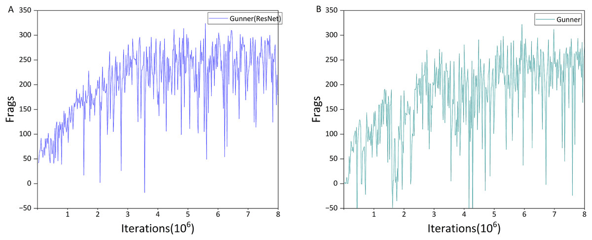
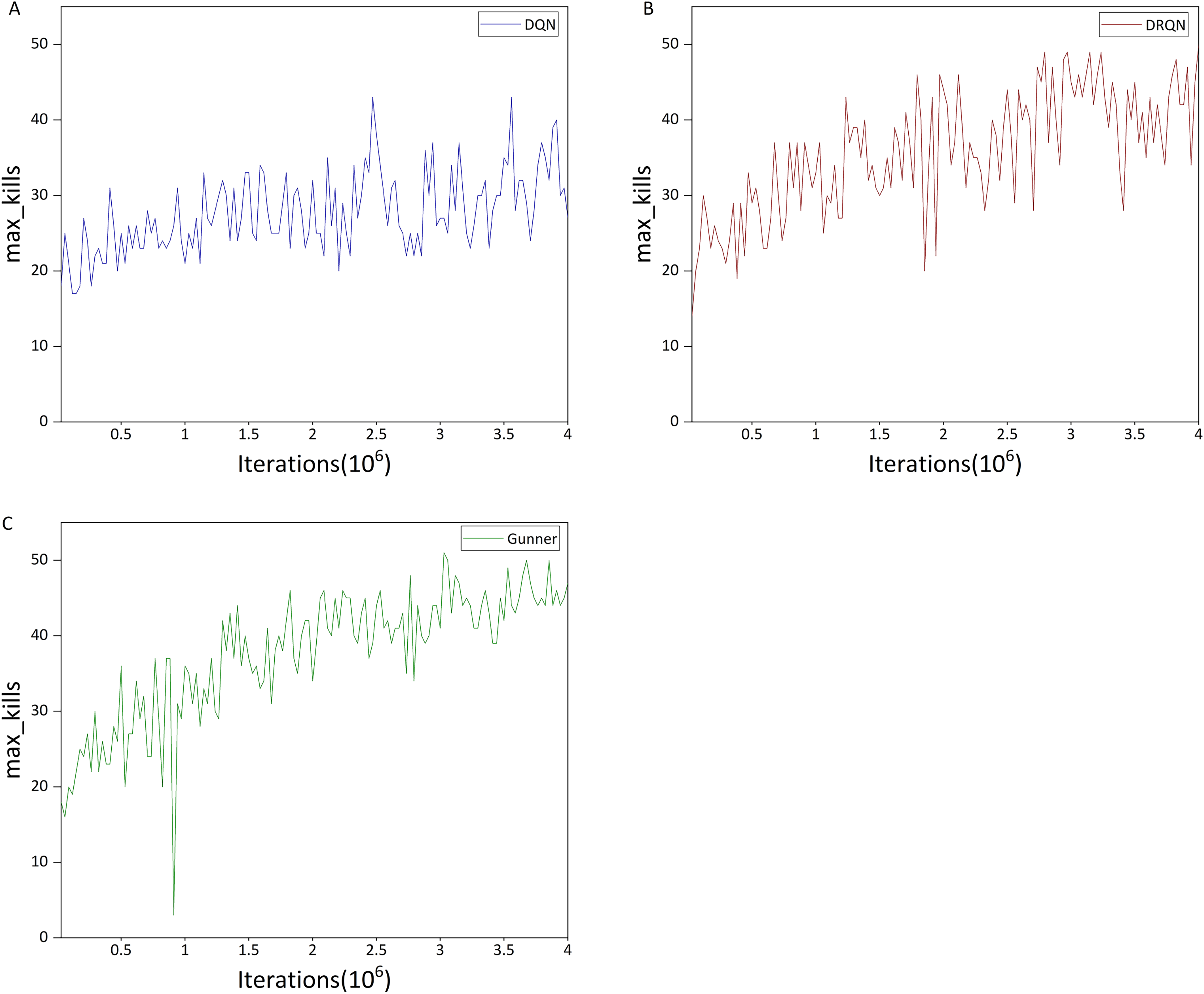
Figure 8: Performance differences between Gunner(ResNet) and Gunner.
ResNet works
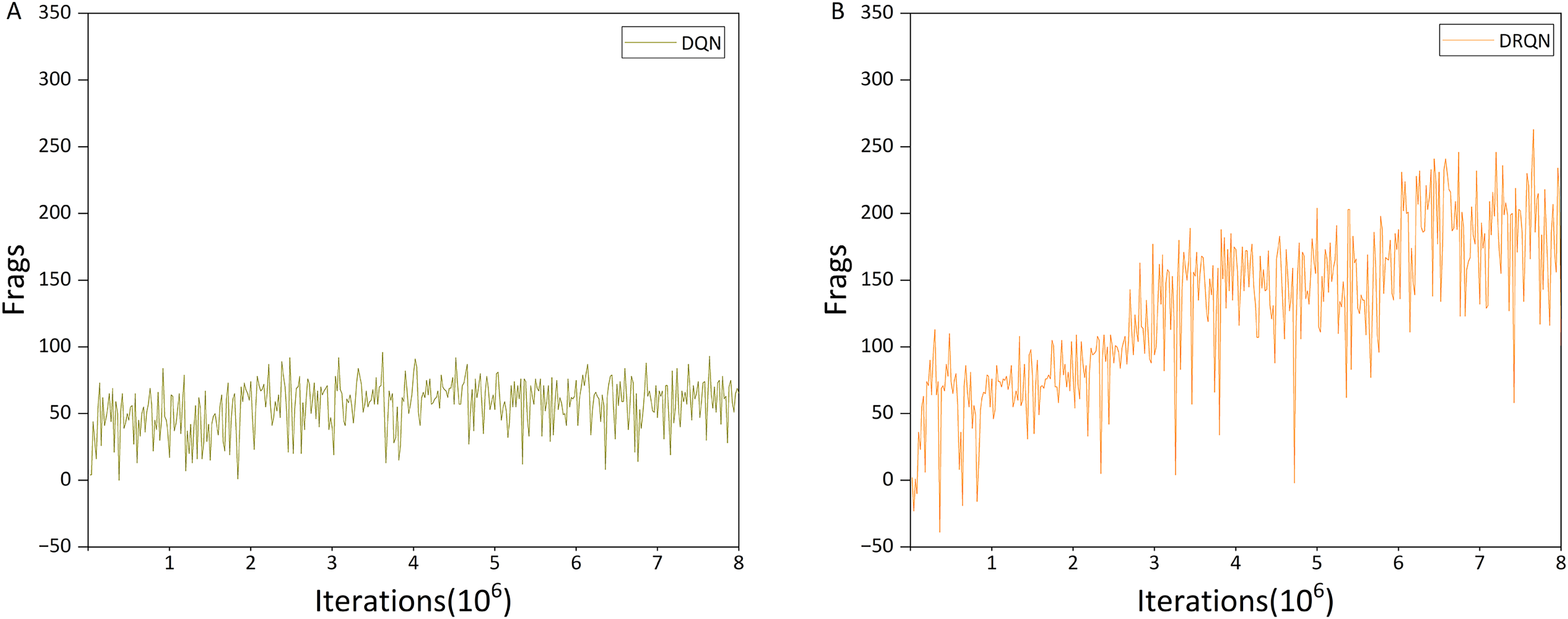
This analysis addresses the first question posed in the Model section. The DRQN model shown in Fig. 9B uses the traditional three-layer CNN architecture, whereas the model in Fig. 7A incorporates the ResNet architecture. Comparison of training results shows that ResNet substantially improves agent performance: after approximately three million iterations, the ResNet-based agent reaches a Frags value of about 250, whereas the CNN-based DRQN achieves less than 200. Even after seven million iterations, the CNN-based agent only reaches 250 Frags. This improvement is likely due to ResNet’s deeper architecture and greater number of parameters, which allow the agent to process a larger state space and make more informed decisions.
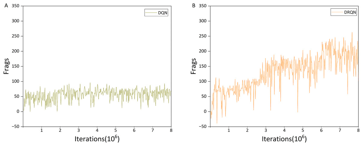
Figure 9: Performance differences between DQN and DRQN.
LSTM is still strong in RL
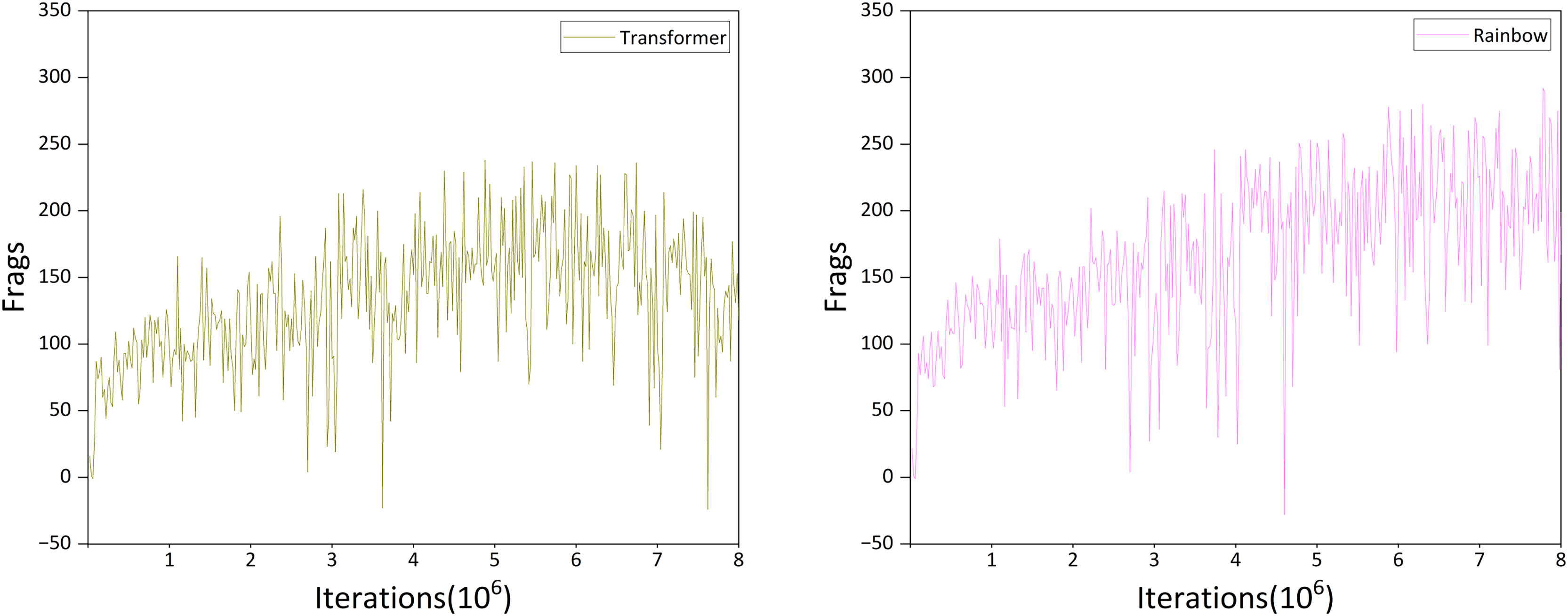
To address the second question posed in the Model section, we evaluated the use of a standard Transformer (Parisotto et al., 2020) as the memory unit in a DRQN agent on Doom. Surprisingly, even after two million iterations, the Transformer-based agent achieved only 24 Frags, considerably lower than the simple DQN baseline (Fig. 9A). We further implemented the publicly available Transformer Encoder model proposed by Sopov & Makarov (2021), referred to here as the Transformer algorithm. The performance of this agent is presented in Fig. 10A.
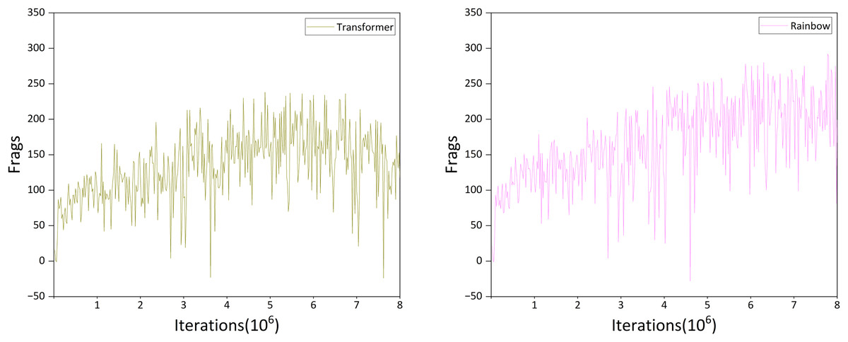
Figure 10: Performance of transformer and rainbow algorithm.
Analysis of Fig. 10A indicates that the Transformer algorithm substantially outperforms the standard Transformer architecture. The agent exhibits a clear learning trajectory rather than random behavior, demonstrating the potential of the Transformer architecture as a memory unit in reinforcement learning.
Returning to the second question, comparison of Figs. 10A and 9B shows that although the Transformer algorithm reaches approximately 200 Frags after about 3 million iterations, its performance plateaus thereafter. In contrast, the DRQN agent reaches the same level after roughly 5.5 million iterations, but continues to improve over the subsequent 2.5 million iterations. Consequently, within eight million iterations, DRQN achieves a maximum Frags value of 263, surpassing the Transformer algorithm’s maximum of 238.
From the comparison of these results, we conclude that in the Doom deathmatch scenario, LSTM outperforms Transformer as a memory unit in reinforcement learning. However, this finding may not generalize to other game scenarios or RL tasks, as also noted by Sopov & Makarov (2021).
In recent years, several Transformer variants specifically designed for reinforcement learning have been proposed. These architectures incorporate modifications to better capture temporal dependencies, demonstrating strong performance in typical RL tasks, such as Gated Transformer-X (Parisotto et al., 2020) and PDiT (Mao et al., 2023). Exploring the application of such RL-optimized Transformer variants as memory units in the Doom game represents a promising direction for future work.
Compared to rainbow
In addition to the aforementioned algorithms, we selected Rainbow as a baseline for comparison. The version used in this study is based on LSTM, commonly referred to as Recurrent Rainbow. Given DQN’s limited performance in the deathmatch scenario, the standard Rainbow was not expected to perform well. Moreover, due to technical constraints encountered during replication, we excluded the Multi-step Learning and Distributional RL components to ensure better integration with our experimental framework. The training performance of this adapted Rainbow is presented in Fig. 10B.
We first compare the training performance of Rainbow and DRQN. As shown in Figs. 9B and 10B, within the first three million iterations, DRQN achieved Frags values primarily in the range [50, 100], whereas Rainbow reached [70, 180], indicating faster convergence of Rainbow during early training. In the intermediate phase (three to six million iterations), DRQN’s Frags values were mostly in [100, 200], while Rainbow ranged from [100, 250], reflecting a larger performance spread and higher Frags values. This difference is likely attributable to Rainbow’s Noisy Networks exploration mechanism, which enables more extensive policy exploration compared to DRQN. In the later stage of training, DRQN reached [150, 230] while Rainbow achieved [200, 280], with a maximum Frags value of 289 for Rainbow compared to 263 for DRQN. Overall, Rainbow consistently attains higher performance throughout the training process.
We next compare the training performance of Gunner and Rainbow (Figs. 10B and 8B), which can be divided into three stages. In the early stage, Gunner exhibits greater performance oscillations, experiencing a notable drop between 1.5 and 2.5 million iterations, yet still reaches over 250 Frags by the end of this stage. In contrast, Rainbow is more stable but only surpasses 200 Frags in the later part of the early stage. During the mid-stage, Rainbow’s Frags remain generally below 250, whereas Gunner exceeds 250 Frags on more than 15 occasions, reaching a peak of 322 Frags toward the end of this stage. In the late stage of training, Rainbow attains a maximum of 289 Frags, approximately 33 Frags lower than Gunner, indicating a notable performance advantage for Gunner.
Regarding training performance, Rainbow demonstrates clear improvements over DRQN in terms of both stability and maximum Frags values. However, when compared with Gunner, these gains are relatively modest. Although Gunner exhibits greater volatility during training, the Frags achieved by the trained agent substantially exceed those of Rainbow, indicating that Gunner attains superior performance in the deathmatch scenario.
Race in the same field
To more accurately and intuitively evaluate the performance of each algorithm, we conducted head-to-head tests for agents trained using six algorithms: DQN, DRQN, Rainbow, Gunner(ResNet), Gunner, and Transformer. Each agent participated in five independent matches, with the final performance determined by the average over these five runs. Each match lasted 900 s. The results of this competition are summarized in Table 3.
| Evaluation metric | DQN | DRQN | Rainbow | Transformer | Gunner(ResNet) | Gunner |
|---|---|---|---|---|---|---|
| Number of kills | 114 | 274 | 310 | 261 | 325 | 345 |
| Number of deaths | 98 | 130 | 126 | 126 | 129 | 119 |
| Number of suicides | 23 | 20 | 26 | 24 | 31 | 33 |
| Number of props | 30 | 73 | 128 | 81 | 87 | 134 |
| Frags value | 91 | 254 | 284 | 237 | 294 | 312 |
| Kill to death ratio | 1.163 | 2.108 | 2.460 | 2.071 | 2.519 | 2.899 |
From Table 3, it is evident that DQN underperforms relative to the other algorithms. Although the DQN-trained agent exhibits the fewest deaths, its overall performance—considering the number of kills and resource acquisitions—remains poor. This phenomenon can be attributed to the agent’s limited exploration behavior, analogous to the “Voldemort” effect observed in games such as PlayerUnknown’s Battlegrounds, where the agent tends to remain confined to a restricted area. The weak performance of DQN is closely associated with the constrained capacity of its fully connected layer, which serves as the memory unit.
The agent trained using DRQN, which incorporates an LSTM as the memory unit, demonstrates substantially stronger performance than DQN, particularly in terms of K/D ratio and the number of props acquired. This improvement can be attributed to the superior memory capacity provided by the LSTM unit. When compared to the Transformer algorithm, the performance gap is less pronounced. The DRQN-trained agent maintains a clear advantage over the Transformer algorithm in both the number of kills and the number of suicides, even achieving the lowest suicide count among the five evaluated algorithms. However, in terms of resource collection, DRQN falls approximately 10% short of the Transformer algorithm, indicating that the Transformer Encoder used as the memory unit in the Transformer algorithm has potential benefits in route planning and item acquisition.
Comparing the measured performance of Rainbow and DRQN, we observe that the improvement in Frags achieved by the Rainbow-trained agent is primarily driven by increases in both the number of kills and props collected. This suggests that the components integrated into Rainbow play a significant role in enhancing these aspects. When compared with Gunner(ResNet), although Rainbow’s kill count remains lower, it demonstrates substantial progress in props acquisition, which we attribute largely to differences in exploration strategies. Finally, in comparison with Gunner, Gunner exhibits superior performance in kills, deaths, and K/D ratio, while Rainbow’s performance in props acquisition is relatively close to that of Gunner, indicating that Gunner achieves a more balanced overall performance across multiple evaluation metrics.
Gunner(ResNet) is a variant of Gunner with Noisy networks removed. As discussed in the ‘Dueling networks has another function’ section, its performance is similar to the model without Dueling networks. The main performance difference between Gunner(ResNet) and DRQN lies in the use of the scalable network architecture. According to Table 3, employing the ResNet architecture improves the agent’s performance primarily through an increase in the number of kills, while the improvement in props acquisition is modest. This may be attributed to the deeper network architecture providing the agent with greater capacity to identify enemies compared to the traditional three-layer CNN. The modest improvement in props acquisition is likely due to differences in the agent’s exploration mechanism.
The best-performing agent in the entire competition is clearly the one trained using the Gunner algorithm. It outperforms all other algorithms in terms of the number of kills, K/D ratio, and props acquired. Comparing the performance of Gunner(ResNet) and Gunner, it is evident that the integration of Noisy networks substantially increases the number of props obtained, analogous to how the use of ResNet mainly improves the number of kills. This highlights the effectiveness of the exploration mechanism introduced by Noisy networks over the traditional ε-greedy strategy, enabling the agent to discover better policies, as well as the contribution of Dueling networks in stabilizing policy learning.
Table 4 summarizes the performance statistics of six algorithms. Overall, Gunner(ResNet) achieved the highest mean score of 201.830 with a 95% confidence interval of [194.924–208.736], while the standard Gunner model also performed strongly with a mean of 169.895 and a confidence interval of [161.750–178.040]. These results clearly surpass the remaining methods, including Rainbow (165.803), Transformer (133.025), DRQN (129.297), and DQN (57.672). The confidence intervals of the Gunner-based models show limited overlap with those of the non-Gunner algorithms, indicating that their superior performance is not only consistent but also statistically reliable. While the baseline methods display moderate to high variability, the Gunner variants maintain both higher scores and robust confidence intervals. Taken together, these findings demonstrate the clear advantage of the Gunner architecture—particularly when removing Noisy networks—in enhancing performance across the evaluated environment.
| Algorithm | Mean | Standard deviation | 95% confidence interval |
|---|---|---|---|
| DQN | 57.672 | 19.111 | [55.993–59.351] |
| DRQN | 129.297 | 57.346 | [123.667–134.927] |
| Rainbow | 165.803 | 57.852 | [160.116–171.489] |
| Transformer | 133.025 | 48.023 | [128.305–137.745] |
| Gunner | 169.895 | 82.858 | [161.750–178.040] |
| Gunner(ResNet) | 201.830 | 70.257 | [194.924–208.736] |
Additional experiments
In the additional experiments, we focus on two Doom scenarios: Health Gathering Supreme and Defend the Center. Although these scenarios are simpler than the deathmatch scenario, they provide a clearer evaluation of the algorithm’s performance in specific aspects and its generalization to other Doom scenarios. In this section, DQN and DRQN are used as baseline algorithms for comparison.
Health gathering supreme
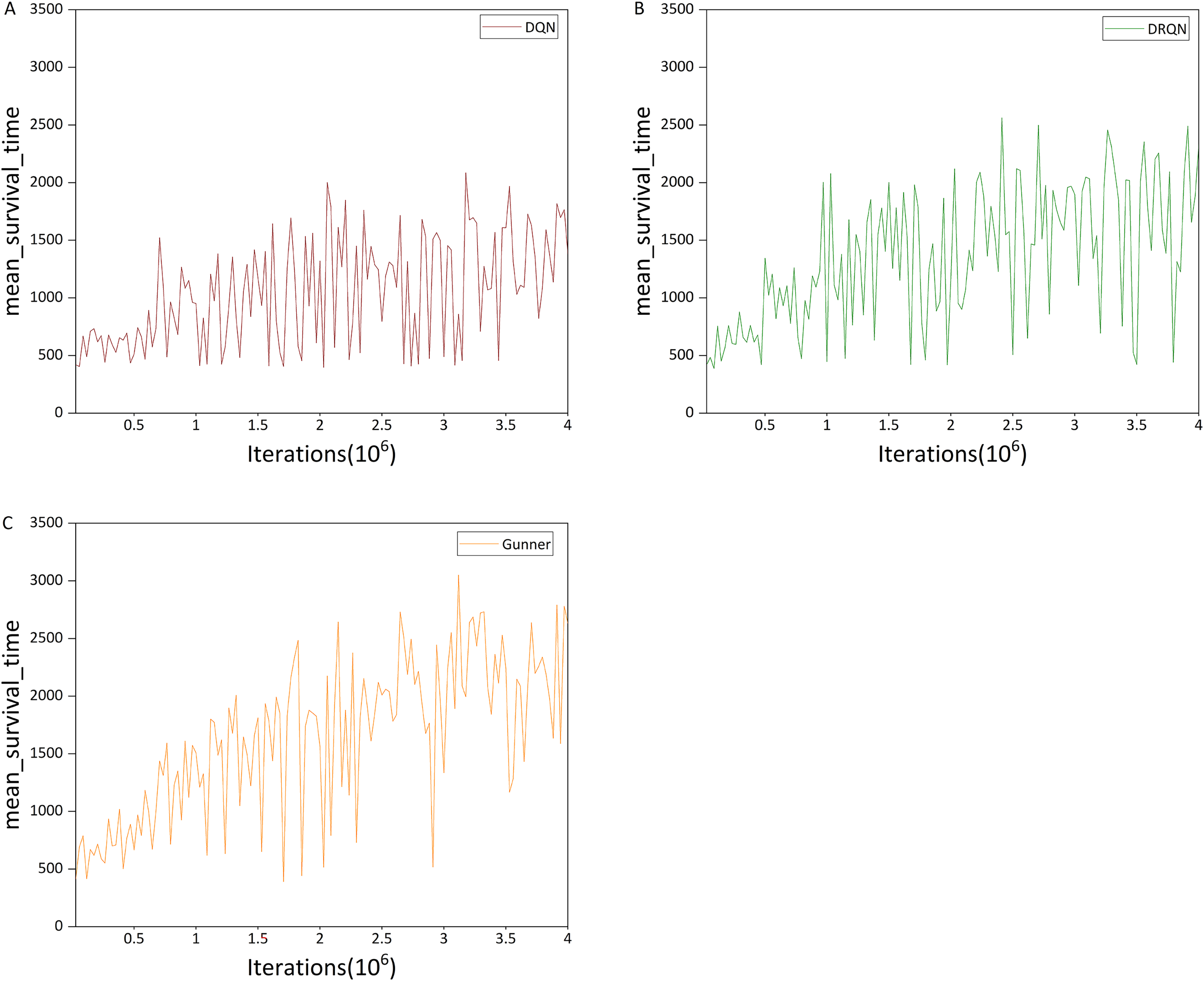
The first experiment was conducted on the Health Gathering Supreme (HG) scenario. We ran the three algorithms for four million iterations and evaluated performance using the agents’ mean survival time within evaluation intervals of 30,000 iterations as the primary metric, with the maximum survival time recorded as a supplementary metric. Mean and maximum survival times of the agents are shown in Figs. 11 and 12, respectively.
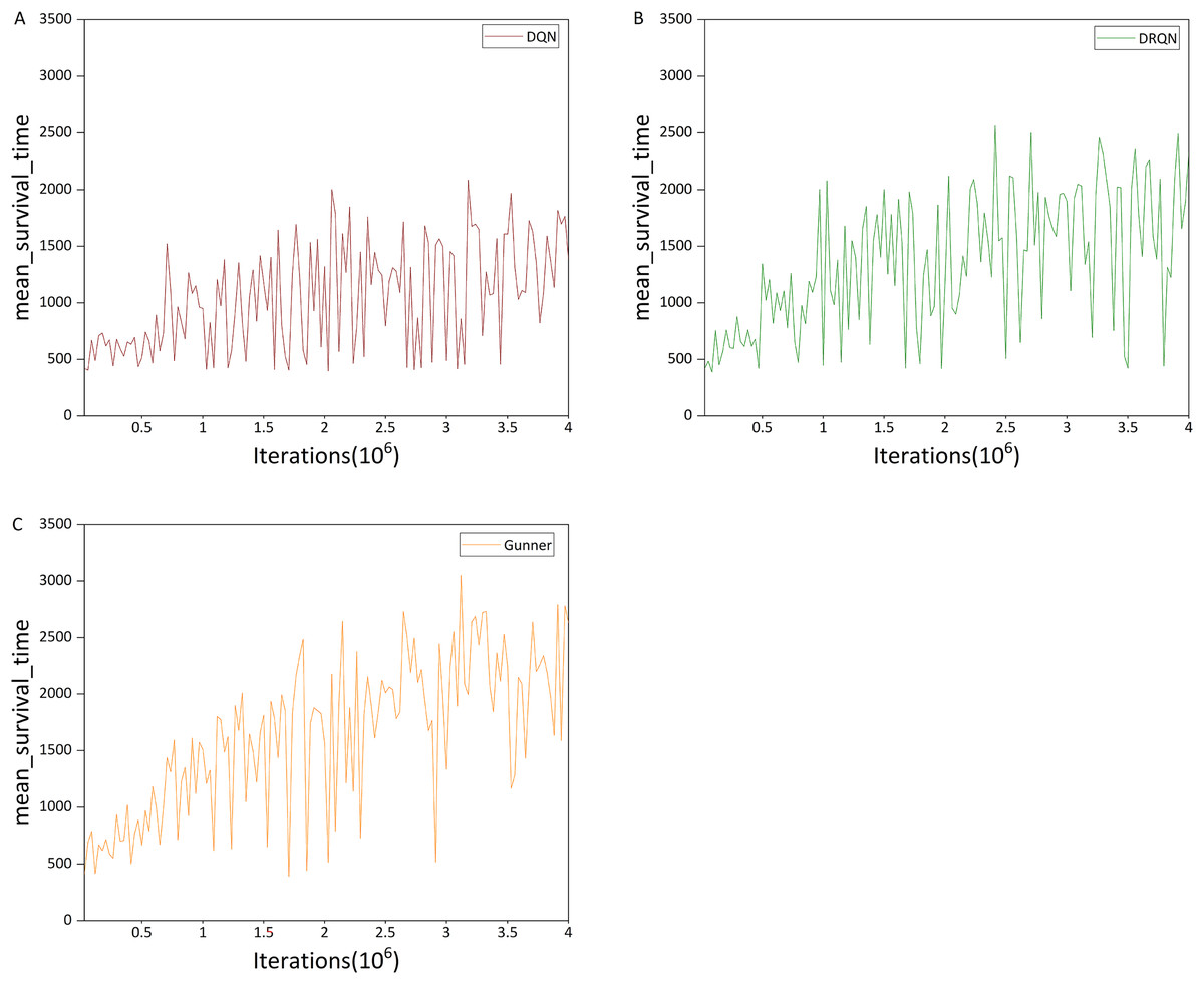
Figure 11: (A–C) Mean survival time in the HG scenario.
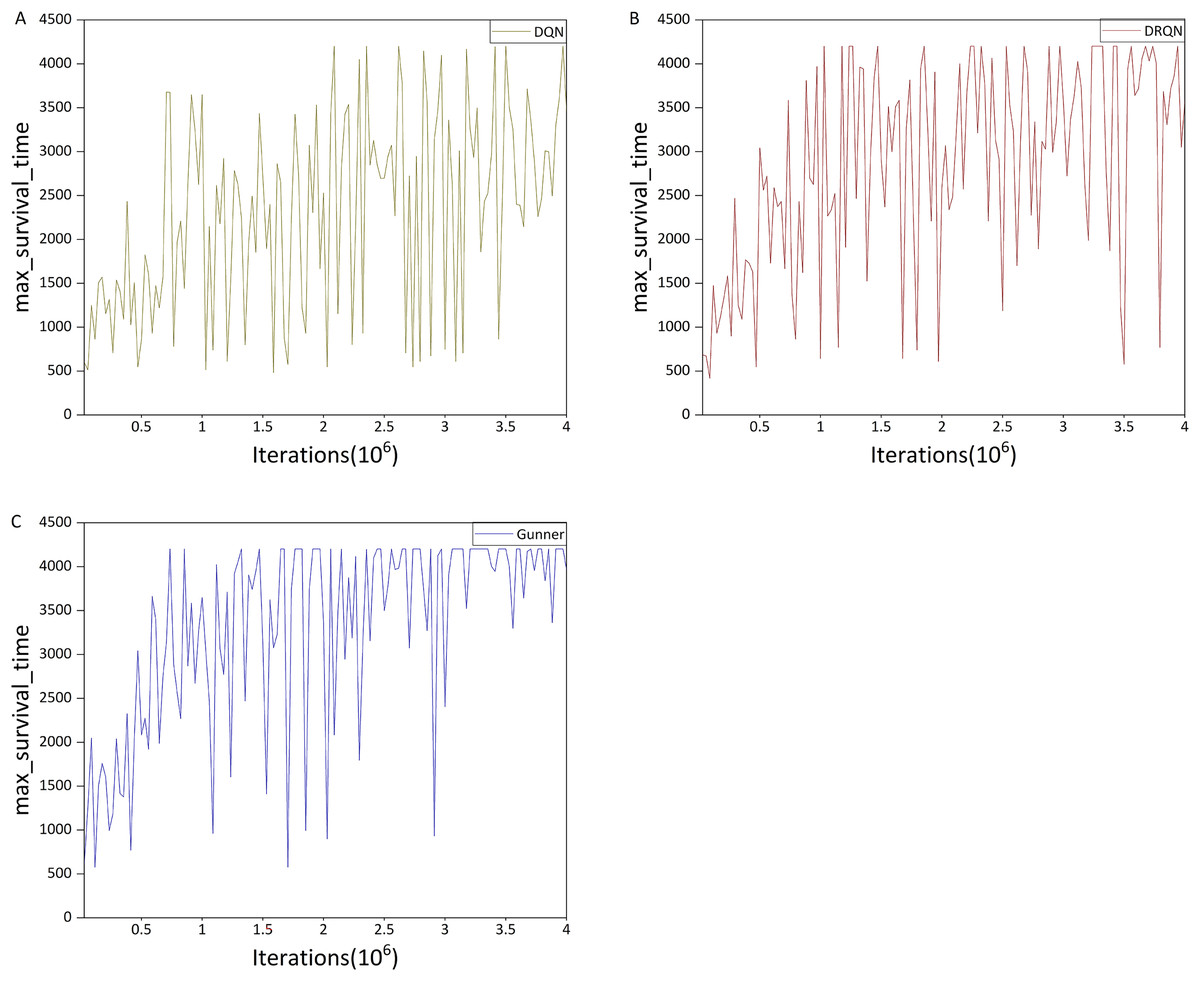
Figure 12: (A–C) Max survival time in the HG scenario.
Figure 11A shows that DQN performs significantly better in the HG scenario than in the deathmatch scenario, exhibiting a clear upward trend, in contrast to the fluctuating performance observed in the deathmatch scenario. Although the HG scenario still has complex maps compared to deathmatch, its gameplay is relatively simple, requiring the agent only to collect props without complex map planning, which is manageable for DQN to learn. Fig. 12A shows that DQN reaches the maximum survival time within a single evaluation interval (4,201 time steps). However, compared with DRQN (Fig. 12B), only a few rounds achieve this maximum value. Comparing Figs. 11B and 11A, at 1 million iterations, DRQN achieved a 2,000+ mean survival time steps, and reached or exceeded this value about 15 times in subsequent iterations, while DQN only approached this value 3 times. In terms of the maximum value of the average survival time, DRQN also has a maximum of 2,563.45 time steps, which is 22.9% more than the DQN’s 2,085.7 time steps.
We next examine the performance difference between Gunner and DRQN, focusing first on the maximum survival time. Figure 12C shows that the two curves are similar during the first 1.5 million iterations. However, in later iterations, Gunner reaches the optimal value more frequently and gradually stabilizes between 3,500 and 4,201 time steps after 3 million iterations, whereas DRQN remains below 3,000 time steps.
Figure 11C shows that in terms of mean survival time, Gunner reaches an average of 2,500 time steps after about 1.8 million iterations, while DRQN only reaches this level after about 2.4 million iterations. Regarding maximum mean survival time, Gunner achieves 3,050.95 time steps, approximately 38.5% higher than DRQN’s 2,563.45. This improvement exceeds that observed between DRQN and DQN. In the later stages of algorithm iteration, Gunner’s mean survival time remains largely above 2,000 time steps, whereas DRQN stays above 1,500 time steps. Through comparison with DRQN and DQN, these results demonstrate that Gunner consistently achieves superior performance in the HG scenario.
Figure 11C shows that in terms of mean survival time, Gunner reaches an average of 2,500 time steps after approximately 1.8 million iterations, whereas DRQN reaches this level only after about 2.4 million iterations. Regarding maximum mean survival time, Gunner achieves 3,050.95 time steps, approximately 38.5% higher than DRQN’s 2,563.45. This improvement exceeds the difference observed between DRQN and DQN. In the later stages of the algorithm iteration, Gunner’s mean survival time remains largely above 2,000 time steps, while DRQN stays above 1,500 time steps. Through comparison with DRQN and DQN, these results demonstrate that Gunner consistently achieves superior performance in the HG scenario.
Defend the center
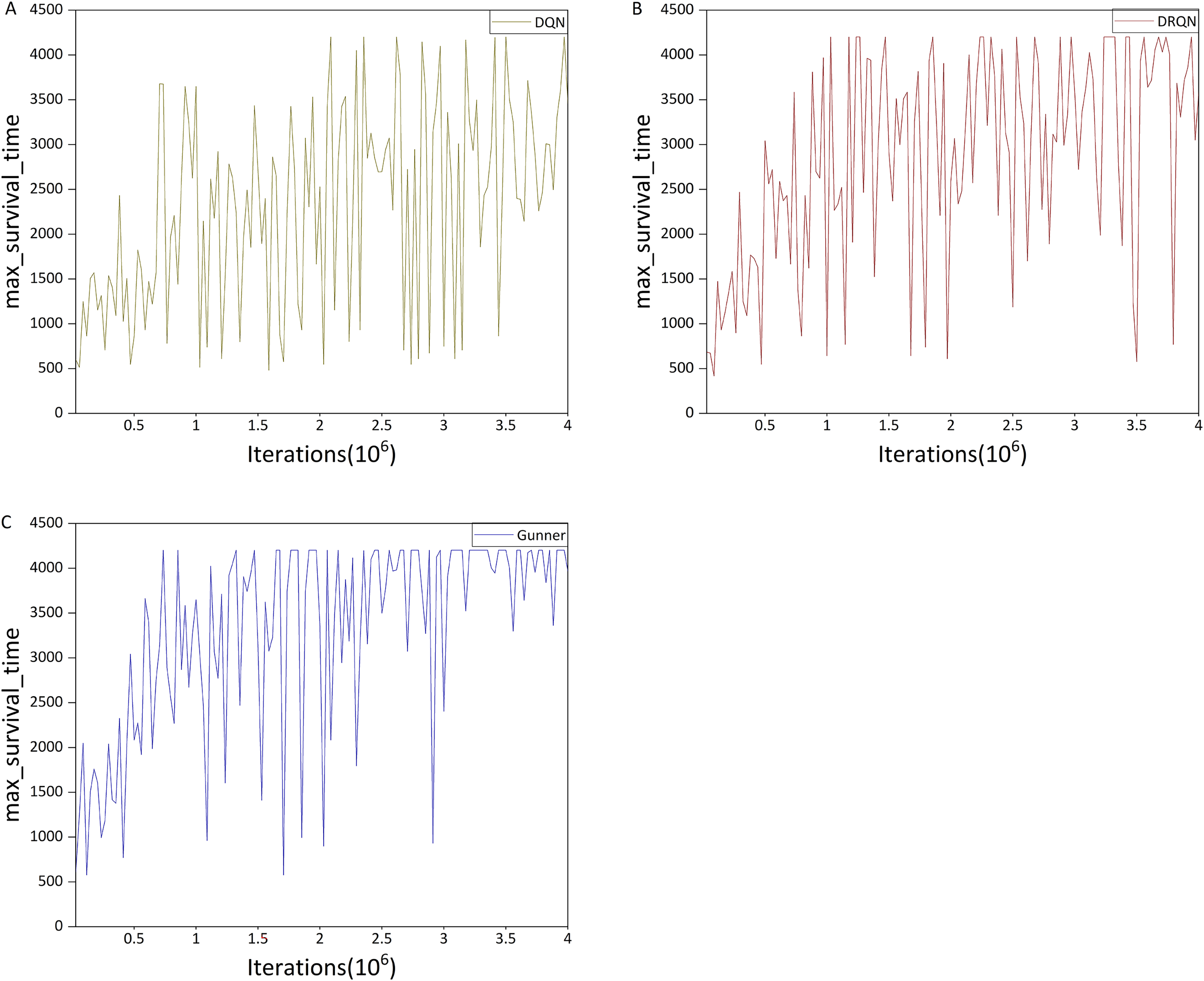
The second part of the additional experiments focused on the Defend the Center (DC) scenario, which primarily tests the algorithm’s ability to detect and eliminate targets, as described in “scenario” section. In this experiment, the three algorithms were trained for 4 million iterations, and the mean and maximum number of kills per round were recorded within evaluation intervals of 30,000 iterations. The results are shown in Figs. 13 and 14.
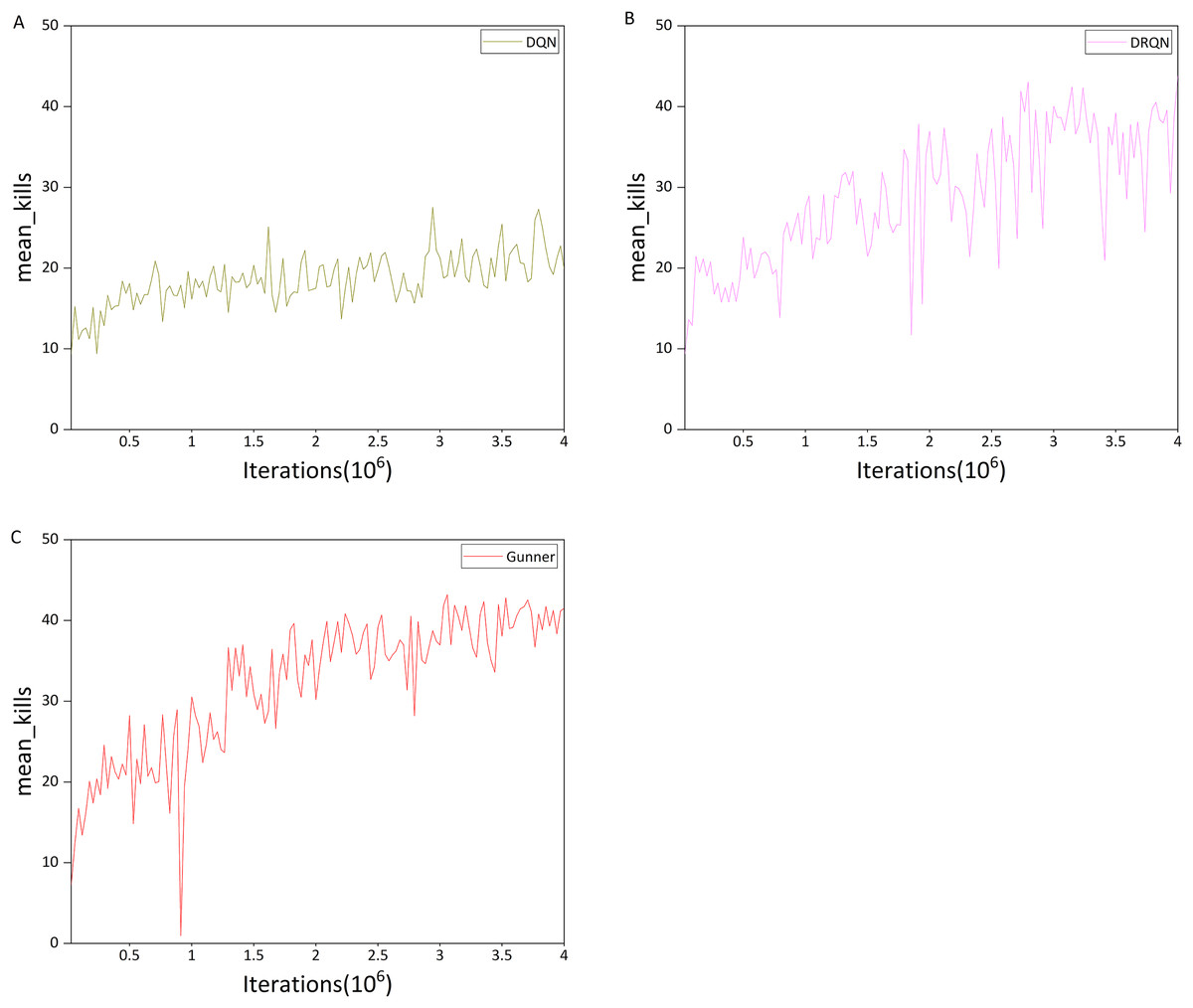
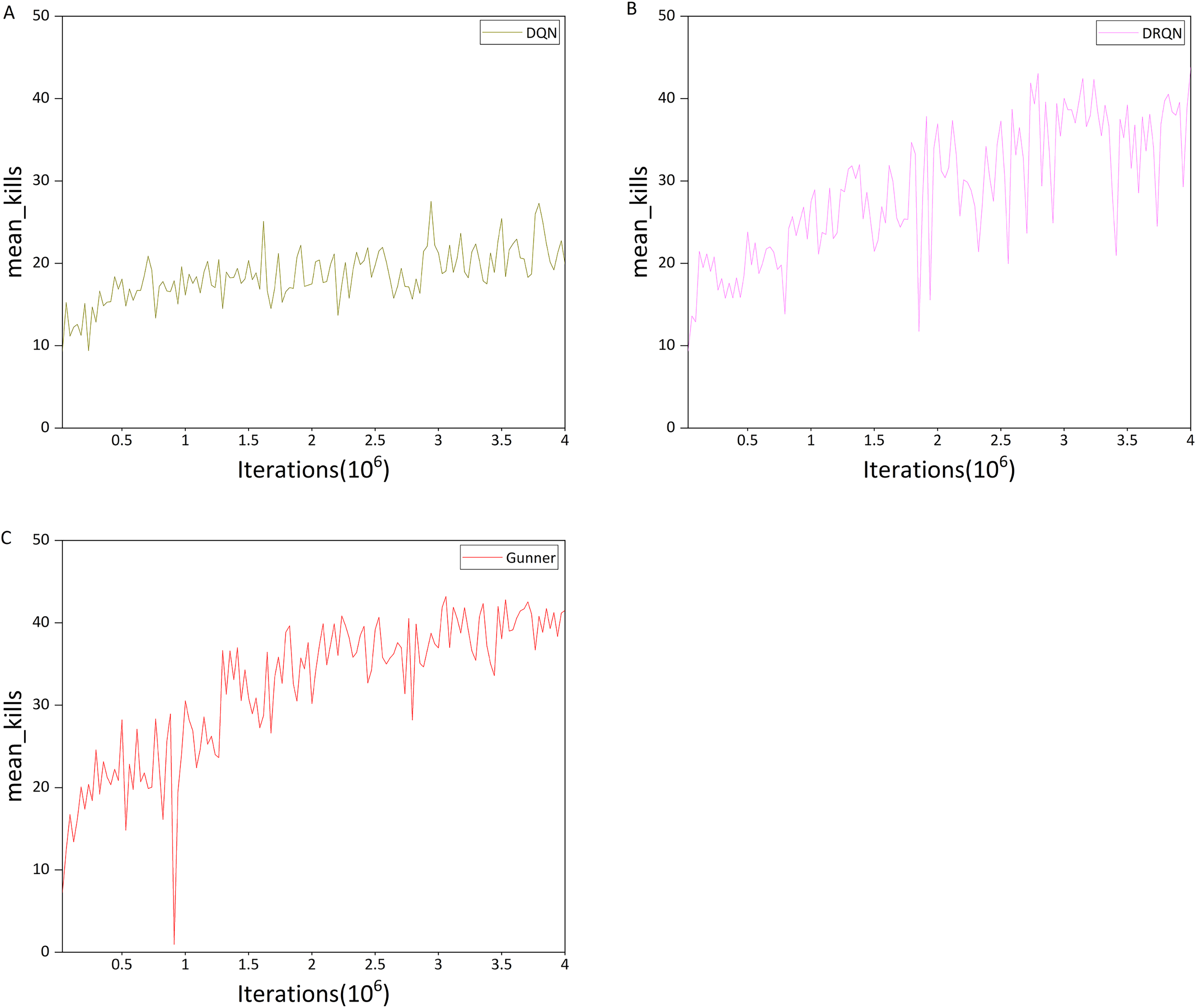
Figure 13: (A–C) Mean kills in the DC scenario.
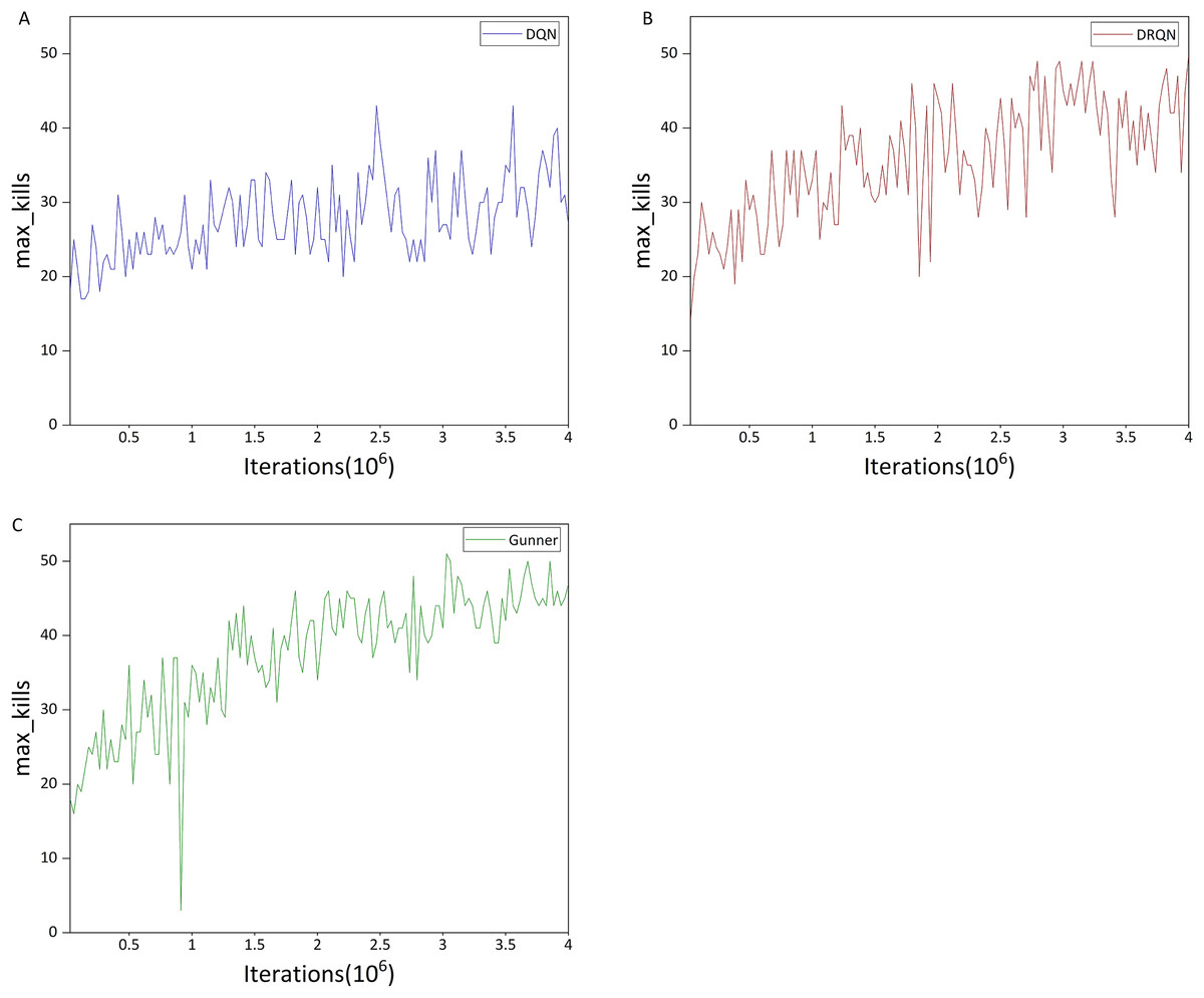
Figure 14: (A–C) Max kills in the DC scenario.
Comparison of Figs. 13A and 13B indicates that the upward trend of DQN is significantly weaker than that of DRQN, and it is also much weaker than in the previous HG scenario. In addition, the maximum mean kills per round for DQN is only 27.55, whereas DRQN achieves 43.05, representing a 56.26% improvement over DQN. This may explain DQN’s poor performance in the deathmatch scenario, which can be attributed to the relatively limited ability of DQN to detect and locate targets in a 3D environment.
This is also evident from the maximum number of kills per round, as shown in Figs. 14A and 14B. For DQN, the maximum number of kills is mostly within the range of 20–40, whereas DRQN is mostly within 30–50. DRQN clearly outperforms DQN in this metric.
We next examine Gunner’s performance, focusing first on the mean number of kills. Comparison of Figs. 13C and 13B indicates that during the first one million iterations, the performance difference between the two algorithms is relatively small. The difference becomes evident after 1.5 million iterations. From then until 4 million iterations, the oscillation amplitude of Gunner’s mean kills curve does not exceed 10 kills, whereas DRQN exhibits much larger oscillations.
Furthermore, the oscillation amplitude of Gunner’s kills did not exceed 5 after 3 million iterations, indicating that the curve is approaching convergence. Both algorithms exhibit nearly identical maximum mean kills, with Gunner at 43.2 and DRQN at 43.05. Taking into account potential game variability, their performance in this metric can be considered similar. This can be explained by the relatively simple scenario pattern, which allows both algorithms to reach near-optimal performance.
In terms of maximum kills per round, both algorithms exhibit similar performance curves, both reaching a maximum of 50 kills. However, Gunner’s curve is closer to convergence than DRQN’s. During the second half of the training process, Gunner’s oscillations do not exceed 10 kills, whereas DRQN exhibits oscillations of around 20 kills. This trend is more pronounced in the last 500,000 iterations, where Gunner’s performance curve approaches convergence, whereas DRQN still exhibits substantial oscillations.
The experimental results demonstrate that Gunner continues to perform well in the DC scenario. Across these three Doom game scenarios, these results suggest that Gunner is capable of handling the 3D environment of the game and achieving strong performance in target recognition and route planning tasks.
Gunner(ResNet) vs Gunner
In the final part of the Additional Experiments section, we examine the average performance of Gunner and Gunner(ResNet) under different random seeds. We conducted three independent trials for each model, training them for eight million iterations in the deathmatch scenario. Experiments were conducted on a system equipped with a 12-vCPU Intel(R) Xeon(R) Platinum 8336C CPU and dual RTX 2080 Ti GPUs (22 GB each). Under these configurations, both models required approximately four days to complete training. The training results are presented in Fig. 15.
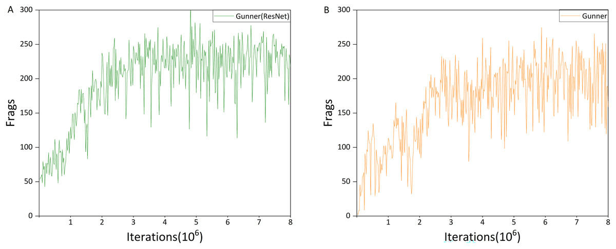
Figure 15: (A and B) Average performance of Gunner(ResNet) and Gunner.
Figures 15A and 15B present the average performance of Gunner(ResNet) and Gunner across three random seeds, respectively. The training process can be divided into three phases. In the first three million iterations, Gunner(ResNet) exhibited a more pronounced upward trend, without the performance dip between one and three million iterations that is typically observed in Gunner’s training curves. Since the primary distinction between the two algorithms lies in their exploration mechanisms, this early performance drop in Gunner can largely be attributed to the use of Noisy networks.
Between three and six million iterations, Gunner(ResNet)’s training performance began to converge, stabilizing between 200 and 250 Frags, whereas Gunner’s performance remained concentrated between 150 and 230 Frags. In the final two million iterations, Gunner(ResNet)’s results remained largely unchanged, indicating convergence. By contrast, while Gunner also appeared to stabilize, its performance continued to fluctuate substantially, with oscillation amplitudes of approximately ±100 Frags, compared to about ±50 Frags for Gunner(ResNet). These results suggest that the exploration strategy introduced by Noisy networks contributes to notable performance differences among agents.
While the overall training performance curves indicate that Gunner(ResNet) outperforms Gunner (Fig. 8), the ultimate goal of training is to obtain an agent that performs optimally in the Doom environment. Owing to the oscillatory behavior introduced by Noisy networks, Gunner occasionally produces agents that achieve higher Frag scores during actual testing—an outcome not observed with Gunner(ResNet).
Finally, we report the average performance with standard deviations across trials. Gunner(ResNet) achieved a mean of 197.169 ± 71.119, whereas Gunner achieved a mean of 164.893 ± 75.980.
Discussion
Kempka et al. (2016) developed the VizDoom AI research platform and evaluated the performance of DQN in two simple Doom scenarios. Wu & Tian (2022) employed the A3C algorithm, enhanced with reward shaping and curriculum design, to train the agent F1, which won first place in the 2016 VizDoom Competition Track 1. Lample & Chaplot (2017) combined the DRQN algorithm with additional improvements, such as frame-skip technology and a game features network, to train the agent Arnold for the deathmatch scenario, achieving first place in the 2017 VizDoom Competition Track 2. Sopov & Makarov (2021) explored replacing the LSTM memory unit with a Transformer encoder within the A3C framework; however, the resulting agent performed poorly compared to LSTM in Doom’s deathmatch scenario. Li et al. (2023) proposed a multi-stage learning framework that achieved state-of-the-art results in previous VizDoom AI Competitions, albeit with relatively high computational resource requirements. Khan et al. (2024) assessed the performance of several RL algorithms in three simple VizDoom scenarios, demonstrating the platform’s practical utility.
Beyond merely aggregating existing DRL techniques, Gunner provides several novel insights. (1) Our controlled ablation studies reveal non-trivial interactions among components: although Dueling Networks alone contributed minimal improvement, their combination with Noisy Networks stabilized exploration and prevented policy collapse—a phenomenon rarely documented in prior work. (2) Replacing the shallow CNN backbone with a deeper ResNet significantly enhances representation learning in visually complex 3D environments such as Doom. This observation suggests that, unlike in 2D Atari domains where shallow encoders often suffice, high-dimensional and partially observable tasks benefit from deeper architectures that capture richer spatial features. (3) Experiments in the Doom deathmatch scenario show that directly using a standard Transformer as the memory unit results in performance inferior to that of LSTM. Despite the growing interest in Transformer-based models, this finding indicates that the unmodified Transformer is less stable and less effective at handling the rapid dynamics and partial observability characteristic of Doom’s competitive FPS environment. Collectively, these results highlight that Gunner is not merely an empirical improvement but a framework that demonstrates how representation, memory, and exploration modules must be carefully balanced to develop effective 3D RL agents—an insight that extends beyond Doom to other complex environments.
Conclusions
In this article, we proposed Gunner, a novel deep reinforcement learning algorithm, and applied it to the 3D game Doom. Gunner integrates four key components: a scalable network architecture for visual feature extraction, an LSTM module for temporal memory, Dueling Networks for stable value estimation, and Noisy Networks for enhanced exploration. We conducted experiments in three VizDoom scenarios—Deathmatch, Health Gathering Supreme, and Defend the Center—and adopted the AdamW optimizer as the default configuration to improve training stability and efficiency.
In the Deathmatch scenario, we framed our study around two conjectures, both of which were validated through experiments. The results confirmed that employing a scalable network architecture and LSTM as the memory unit substantially enhances the agent’s performance. Furthermore, the contributions of other algorithm components were also empirically verified. Comparative evaluation under identical conditions across five algorithms demonstrated that Gunner significantly outperformed the others in terms of kills, K/D ratio, and item acquisition, highlighting its superior competitive capability in the complex Doom Deathmatch environment. Finally, we also evaluated a Transformer-based RL algorithm. Although the standard Transformer Encoder as the memory unit performed worse than LSTM in this task, it achieved better item acquisition, indicating that Transformer architectures still hold potential for enhancing agent performance in this scenario.
In the Health Gathering Supreme and Defend the Center scenarios, we further evaluated the generalization capability of the algorithm. Comparative experiments show that Gunner consistently outperforms DQN and DRQN across all three scenarios, demonstrating its strong performance in target recognition and route-planning tasks within the Doom environment.
Future work will focus on two directions: (1) integrating Transformer variants that have been shown effective in the RL community as the memory unit, in order to further enhance the algorithm’s memory capacity; and (2) applying the Gunner algorithm to other 3D FPS games to evaluate and improve its cross-platform generalization capability.