
Augmenting medical visual question answering with mixup, label smoothing, and layer-wise relevance propagation eXplainable Artificial Intelligence
- Published
- Accepted
- Received
- Academic Editor
- Paulo Jorge Coelho
- Subject Areas
- Artificial Intelligence, Computer Vision, Data Mining and Machine Learning, Natural Language and Speech, Neural Networks
- Keywords
- Medical visual question answering, VGGNet, ResNet, ImageCLEF, Augmentation, MVQA dataset, eXplainable Artificial Intelligence (XAI), Medical image processing
- Copyright
- © 2026 Noor Mohamed and Srinivasan
- Licence
- This is an open access article distributed under the terms of the Creative Commons Attribution License, which permits unrestricted use, distribution, reproduction and adaptation in any medium and for any purpose provided that it is properly attributed. For attribution, the original author(s), title, publication source (PeerJ Computer Science) and either DOI or URL of the article must be cited.
- Cite this article
- 2026. Augmenting medical visual question answering with mixup, label smoothing, and layer-wise relevance propagation eXplainable Artificial Intelligence. PeerJ Computer Science 12:e3407 https://doi.org/10.7717/peerj-cs.3407
Abstract
The growing volume of medical data presents significant opportunities for advancing Medical Visual Question Answering (MVQA) systems. However, an imbalance in the number and distribution of image and Question–Answer (QA) pairs poses challenges for developing robust models. This study proposes improving existing MVQA datasets using data augmentation techniques specifically Mixup and Label Smoothing—to address this issue. The performance of MVQA models trained on these enhanced datasets is evaluated using quantitative metrics, as well as Layer-wise Relevance Propagation for eXplainable artificial intelligence (LRP XAI). Results indicate that models trained on the augmented datasets outperform those trained on the baseline datasets, showing significant gains in both accuracy and Bilingual Evaluation Understudy (BLEU) score. Furthermore, LRP XAI visualizations highlight key image and text regions that contribute to accurate answer predictions, thereby improving model interpretability and trust. This work underscores the importance of dataset augmentation and explainability in advancing MVQA research and it is available in https://doi.org/10.5281/zenodo.15910714.
Introduction
The Medical Visual Question Answering (MVQA) system leverages computer vision and natural language processing (NLP) to answer questions related to medical images. The answer to a visual question is either open-ended or closed-ended. Open-ended answers provide brief descriptions, while closed-ended answers are typically yes or no. In both cases, answers are generated using information extracted from various regions of the medical images.
The MVQA system is applied in clinical decision-making and serves as a support tool for medical students and physicians. It also assists patients with scotoma or amblyopia by answering medical questions in real time according to their specific needs (Le, Nguyen & Nguyen, 2021). The MVQA system has a significant societal impact; however, several real-time challenges hinder its ability to provide accurate answers for all questions. The primary challenge is improving existing datasets to develop more effective MVQA systems (Jin et al., 2022; Gong et al., 2022; Li et al., 2022).
MVQA datasets collected from various sources face two key challenges: limited overall dataset size and an imbalanced distribution of samples, with very few or disproportionately many samples for certain labels (Nguyen et al., 2019; Lu et al., 2023). To address these challenges, many researchers have recommended augmenting MVQA datasets. Commonly recommended dataset augmentation approaches include: (i) acquiring samples from hospitals and clinics (Lin et al., 2021), (ii) performing geometric transformations such as flipping, rotation, translation, scaling, and shearing (Lu & Chen, 2024), (iii) collecting similar samples from other datasets or generating them from medical textbooks using deep learning techniques, and (iv) reducing overrepresented or underrepresented labels to balance sample distribution. Among these approaches, collecting samples from hospitals is practically difficult due to privacy and ethical concerns. Additionally, geometric transformations are not recommended for medical images, as they can lead to sample misclassification. Therefore, the third and fourth approaches are adopted in the proposed work to enhance the MVQA datasets and build improved MVQA models.
In the proposed work, to address the third approach (dataset scarcity problem), the Path-VQA dataset is generated using a semi-pipeline approach and validated by a pathology expert. Along with this dataset, the VQA-MED 2018, 2019, 2020, and 2021 datasets are also enhanced using mathematical functions combined with Mixup and Label Smoothing techniques to reduce imbalanced labels (fourth approach).
The enhanced datasets generated by these approaches are used to create MVQA models, and their results are validated using quantitative metrics (Evtikhiev et al., 2023) and explainable AI (XAI). The reasons for choosing the semi-pipeline approach, Mixup and Label Smoothing techniques, and the XAI method in the proposed work are discussed in the following paragraph. The semi-pipeline approach is used because it supports parallel processing and efficiently handles large data in less time. The Mixup and Label Smoothing techniques are applied in dataset augmentation as they provide a generic solution with significantly improved performance, regardless of dataset type. The XAI technique is employed in addition to quantitative metrics because it highlights significant regions in the images and key contributing words from the questions for answer prediction.
The novelty of the proposed work includes: (i) addressing dataset scarcity by developing an improved MVQA dataset, (ii) enhancing interpretability by developing an MVQA system capable of answering questions related to different organs, planes, modalities, abnormalities, and more, and (iii) providing a foundation for building real-world deployable systems. This work’s novelty lies not only in augmenting and benchmarking improved datasets but also in its holistic focus on improving performance and educational utility in MVQA. It is among the first studies to combine clinical validation, data-centric augmentation, and visual interpretability for MVQA in pathology and radiology domains.
The remaining part of the article is organized into the following subsections. “Related Works” discusses existing work on MVQA and XAI techniques. “Proposed Design” explains the proposed design with appropriate algorithms and mathematical functions. “Experiments And Results” presents the results and performance analysis using quantitative metrics and XAI, along with the limitations of MVQA datasets. Finally, the article concludes with a summary and suggestions for future work.
Related works
The existing works in MVQA related to dataset augmentation, quantitative metrics for MVQA model analysis, and validation of predicted outcomes from XAI visualizations are discussed, with a summary provided in Table 1.
| Authors and years | Datasets | Techniques | Inferences | Limitations |
|---|---|---|---|---|
| Dataset augmentation | ||||
| Al-Sadi et al. (2021) | VQA-MED 2020 | VGG16 and dataset augmentation techniques | Dataset augmentation regularize the dataset | Scope limited to abnormality type samples |
| Gong et al. (2021) | VQA-MED 2021 | ResNet with curriculum learning | Reduces overfitting in the model | – |
| Liu, Zhan & Wu (2021) | VQA-RAD | VGG16 and GRU | Contrastive learning prevents overfitting to small-scale training data | Dataset limitation is not completely addressed |
| XAI visualization | ||||
| Nazir, Dickson & Akram (2023) | Path-VQA | MVQA techniques, Grad-CAM and SHAP | Grad-CAM visualize RoI in the image that contributes to answer prediction | – |
| Huang & Gong (2024) | VQA-RAD | Transformer with Sentence Embedding (TSE) and Grad-CAM | Requires correlation between keywords and medical information for better visual reasoning | – |
The performance of the MVQA system is improved by training the model on large MVQA datasets. The larger dataset is created by increasing the number of samples per label, which helps reduce dataset limitations to some extent. However, the samples in these datasets are unstructured and exhibit sparse features in certain characteristics (Shen et al., 2024). For this, Al-Sadi et al. (2021) generated samples using the ZCA whitening technique and employed VGG16 to develop an MVQA model for the VQA-MED 2020 dataset, achieving a BLEU score of 0.339. However, Liu, Zhan & Wu (2021) trained large amounts of unlabelled radiology images from the VQA-RAD dataset using contrastive learning with a three-teacher model. In the same year, Gong et al. (2021) utilized curriculum learning for data augmentation and adopted label smoothing to prevent overfitting in the MVQA model developed from the VQA-MED 2021 dataset. Then, Thai et al. (2023) improved the quality of the region of interest in samples from the VQA-MED 2023 dataset. For this, the original image is passed through a series of enhancement procedures before being fed into the image encoder for feature extraction.
However, Liu et al. (2023) used Contrastive Language-Image Pre-Training (CLIP), which combines Vision Transformer (ViT), long short term memory (LSTM), and Label Smoothing, to fine-tune a small number of parameters in the adapter module, resulting in significant improvement. As a result, they achieved an accuracy of 0.758 on the VQA-RAD dataset. In addition, Hu et al. (2024) observed that a large chest X-ray dataset is necessary to construct a large language model (LLM) capable of embedding multi-relationship graphs. Meanwhile, Li et al. (2023) found that Multimodal Augmented Mixup (MAM), which incorporates various data augmentations alongside a vanilla mixup strategy, generates more diverse, non-repetitive data. This approach avoids time-consuming artificial data annotations and enhances model generalization capabilities on the VQA-RAD and Path-VQA datasets. In 2025, Lameesa, Silpasuwanchai & Alam (2025) observed that extracting significant regions from the inputs—both images and question tokens—captures detailed relationships between fragments, leading to models that provide reasonable answers. Furthermore, visualization of the output helps identify reasons behind performance issues, which is discussed in the next paragraph.
The different XAI techniques used for visualization in medical domain are, SHapley Additive exPlanations (SHAP), Local Interpretable Model-Agnostic Explanations (LIME), Layerwise Relevance Propagation (LRP), Class Activation Mapping (CAM) and Gradient-weighted Class Activation Mapping (Grad-CAM). In 2019, Vu et al. (2020) used ResNet, attention mechanism and Grad-CAM for VQA-MED 2019 dataset and analysed that the developed model failed to answer, although succeeded to put a focus on important regions in the corresponding images to answer the questions through Grad-CAM visualization. In 2021, Tjoa & Guan (2020) used CAM and LRP for MED-VQA dataset and observed that the reason for the poor results are analysed from the interpretability output such as heatmaps.
Then, Nazir, Dickson & Akram (2023) stated that the consequences of both false positive and false negative cases are far-reaching for patients’ welfare and cannot be ignored. In 2024, Huang & Gong (2024) observed that visual and textual co-attention in Grad-CAM can increase the granularity of understanding and improve visual reasoning in the VQA-MED 2019 and VQA-RAD datasets. As XAI is an evolving field, it is mostly used alongside medical image classification, as demonstrated by Sarp et al. (2021) and Lotsch, Kringel & Ultsch (2021). Sarp et al. (2021) used LIME together with VGG16 to extract additional knowledge and explanations that can also be interpreted by non-data science experts, such as medical scientists and physicians. Using LIME combined with decision trees, Lotsch, Kringel & Ultsch (2021) stated that the system is able to explain in detail the decisions made by the AI to experts in the field. Beyond these XAI techniques, Concept Relevance Propagation (CRP), Adversarial Perturbations and Analysis, Counterfactual Explanations, and Model-Agnostic Techniques are generally well-suited for either image or text; however, they often face limitations when both inputs are applied to the models (Finzel, 2025).
From these related works, it has been inferred that the dataset augmentation improves the overall performance of the MVQA models and it is visualized using LRP XAI technique. Hence the proposed work concentrates on augmenting MVQA datasets, generating the models from the improved datasets and validating the results using quantitative metrics and LRP XAI technique. Finally, LRP XAI technique is also used to show how two closely related disorders take significant information from different regions of the inputs.
Proposed design
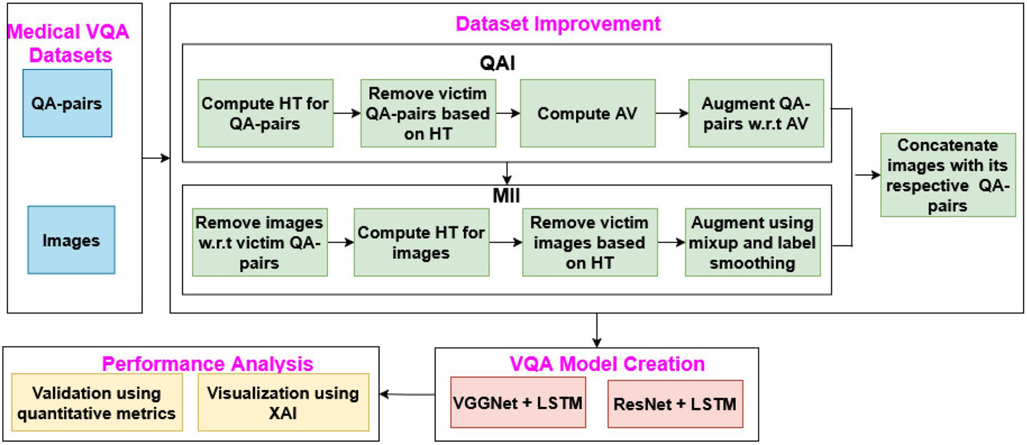
The proposed MVQA system mainly focuses on augmenting MVQA dataset and generating the model from the improved datasets. This process consists of four sequence of steps such as, dataset collection, augmentation of MVQA datasets, MVQA model creation and, validations using quantitative metrics and visualization technique, as shown in Fig. 1. In Fig. 1, QAI, MII, HT, QA pairs, AV, LSTM and XAI represents Question-Answer pairs Improvement, Medical Images Improvement, Hardsample Threshold, Question-Answer pairs, Average Value, long short term memory and eXplainable Artificial Intelligence respectively.
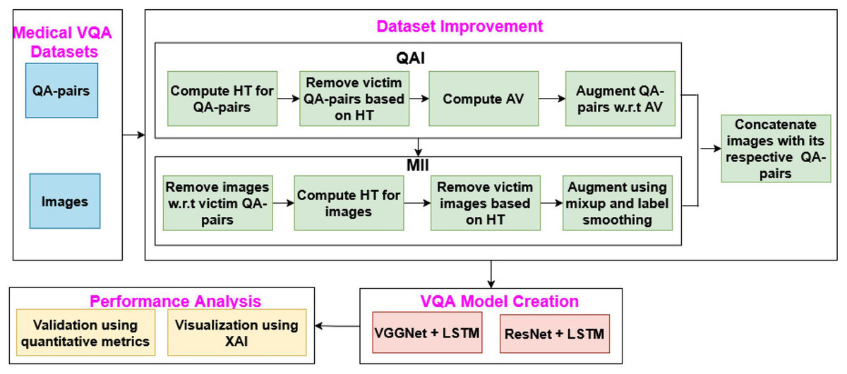
Figure 1: MVQA system design.
In the proposed work, the generated and collected datasets are improved using augmentation approaches such as QAI and MII, which are then used in MVQA model creation. The performance of the MVQA models generated from the original and improved datasets is compared and validated using quantitative metrics and the LRP XAI technique.
MVQA datasets
The MVQA datasets used in this research include the generated medical Path-VQA dataset and collected VQA-MED datasets. The Path-VQA dataset consists of pathological VQA queries collected from online digital libraries and pathology textbooks. The pathology images in the Path-VQA dataset are acquired from the generic textbook named Textbook of Pathology using a semi-automated pipeline approach (Mohan, 2010). The QA pairs associated with this dataset were acquired from He et al. (2020). The images and QA pairs are mapped sequentially, and the annotations are reviewed by a medical annotator.
The VQA-MED datasets are collected from ImageCLEF VQA-MED online forum through the tasks conducted from 2018 to 2021. The number of samples of each dataset are given in the original dataset column of Tables 2 and 3. The VQA-MED 2018 and 2019 datasets consists of radiological images related to different organs, planes, abnormalities and modalities are developed from PubMed Central articles and QA pairs from rule-based question generation system (Hasan et al., 2018; Abacha et al., 2019). The VQA-MED 2020 and 2021 datasets consist of abnormality type visual queries related to different organs are acquired from the MedPix and VQA-MED 2019 datasets (Abacha et al., 2020, 2021). These datasets collected from ImageCLEF provides de-identified, ethically released images, ensuring compliance with privacy standards such as Health Insurance Portability and Accountability Act (HIPAA)/General Data Protection Regulation (GDPR). Moreover, to maintain clinical validity, all augmented samples from the proposed work are reviewed by a certified pathologist. This step ensured that transformations did not alter the diagnostic features or introduce unrealistic artifacts. Only clinically appropriate augmentations were retained for training. These measures were taken to ensure that both the original and augmented data are ethically sourced, medically valid, and suitable for model development. From Tables 2, 3, 4 and 5, these MVQA datasets are represented as D1, D2, D3, D4 and D5 for VQA-MED 2018, VQA-MED 2019, VQA-MED 2020, VQA-MED 2021 and Path-VQA datasets respectively.
| Datasets | Original QA pairs | After Eq. (2) | After Cond. 1 | After Eq. (3) | Enhanced QA pairs | |||
|---|---|---|---|---|---|---|---|---|
| #Samples | #Labels | (HT) | #Samples | #Labels | (AV) | #Samples | #Labels | |
| D1 | 5,913 | 4,461 | 1 | 5,543 | 4,200 | 4 | 5,412 | 4,200 |
| D2 | 14,792 | 1,553 | 8 | 14,329 | 1,432 | 17 | 13,143 | 1,432 |
| D3 | 4,500 | 333 | 12 | 4,125 | 325 | 20 | 4,040 | 325 |
| D4 | 5,000 | 332 | 14 | 4,567 | 319 | 23 | 4,087 | 319 |
| D5 | 26,239 | 883 | 1 | 24,876 | 778 | 4 | 23,856 | 778 |
| Datasets | Original images | Enhanced images | ||
|---|---|---|---|---|
| #Samples | #Labels | #Samples | #Labels | |
| D1 | 2,602 | 4,461 | 2,492 | 4,200 |
| D2 | 3,700 | 1,553 | 3,486 | 1,432 |
| D3 | 4,500 | 333 | 4,040 | 325 |
| D4 | 5,000 | 332 | 4,087 | 319 |
| D5 | 3,998 | 883 | 3,635 | 778 |
| Datasets | Accuracy | BLEU score | ||||
|---|---|---|---|---|---|---|
| OD | ID | SoA | OD | ID | SoA | |
| D1 | 0.161 | 0.276 | – | 0.205 | 0.329 | 0.106(SoA1) |
| D2 | 0.486 | 0.582 | 0.461 (SoA2) | 0.556 | 0.606 | 0.513(SoA2) |
| D3 | 0.248 | 0.263 | 0.361 (SoA3) | 0.292 | 0.299 | 0.409(SoA3) |
| D4 | 0.196 | 0.241 | 0.382 (SoA4) | 0.227 | 0.251 | 0.416(SoA4) |
| D5 | 0.453 | 0.576 | 0.540 (SoA5) | 0.561 | 0.579 | 0.561(SoA5) |
| Datasets | Accuracy | BLEU score | ||||
|---|---|---|---|---|---|---|
| OD | ID | SoA | OD | ID | SoA | |
| D1 | 0.167 | 0.281 | – | 0.231 | 0.341 | 0.106(SoA1) |
| D2 | 0.491 | 0.579 | 0.461 (SoA2) | 0.561 | 0.616 | 0.513(SoA2) |
| D3 | 0.282 | 0.312 | 0.361 (SoA3) | 0.330 | 0.343 | 0.409(SoA3) |
| D4 | 0.218 | 0.303 | 0.382 (SoA4) | 0.254 | 0.304 | 0.416(SoA4) |
| D5 | 0.460 | 0.586 | 0.540 (SoA5) | 0.565 | 0.595 | 0.561(SoA5) |
Augmentation of MVQA datasets
The QA pairs and images of MVQA datasets are improved using proposed augmentation approaches namely, QAI and MII and it is given as Functions 1 and 2 in Algorithm 1.
| Input: Medical images with respective question-answer pairs ( ) |
| Output: Improved datasets ) function MVQA( ) |
| • Function to develop improved datasets |
| • N, the number of samples |
| Normalize the datasets |
| for i → 1 to N do |
| QAI ( ) (see Function 1) |
| MII ( ) (see Function 2) |
| end for |
| if ID of in |
| Concatenate the image with its respective QA-pairs |
| end if |
| return |
| Input: Question-answer pairs of medical images ( ) |
| Output: Improved question-answer pairs in different stages ( function QAI ( ) |
| • Function to improve the question-answer pairs |
| • X, the number of samples in each label (L) |
| LQAP → Compute the ratio of under each label of L (refer Eq. (1)) |
| → Calculate the avg no. of QA pairs in each LQAP (refer Eq. (2)) |
| for i → 1 to L do |
| if (refer Cond. 1) |
| Consider as victim label and remove the respective QA pair(s) |
| • where L(i) is an label and L represents total number of labels |
| else |
| end if |
| end for |
| Compute the ratio of count under each label of Lupd. |
| • The Lupd represents updated label count and it ranges up to upd |
| Calculate the avg no. of QA pairs in each LQAP (refer Eq. (3)) |
| for i → 1 to upd do |
| if (refer Cond. 2) |
| Augment the QA pair(s) till the number of samples under each labels (based on Cond. 1) are equivalent to the value |
| else |
| end if |
| end for |
| return |
| Input: Medical images of question-answer pairs ( ) |
| Output: Improved medical images in different stages ) function MII ( ) |
| • Function to improve the medical images |
| • X, the number of images |
| for n → 1 to N do |
| if has respective question-answer pairs in |
| end if |
| Compute the ratio of count under each label of L |
| Calculate the avg no. of images in each LIM |
| for i → 1 to upd do |
| if (refer Cond. 3) |
| Consider as victim label and remove respective images |
| • where L(i)is an ith label and upd represents updated number of labels from QAI |
| else |
| end if |
| end for |
| Compute the ratio of count under each label of Lupd |
| Calculate the avg no. of images in each LIM |
| • The Lupd represents updated label count and it ranges up to upd |
| for i → 1 to upd do |
| if (refer Cond. 4) |
| Augment the images by LS and MU techniques until the image count under each labels are equivalent to value |
| else |
| end if |
| end for |
| end for |
| return |
The mathematical parameters used in Algorithm 1 are: let X be the input consists of both Question-Answer pairs (QAP) and Images (IM) i.e., consists of and corresponding . The labels are represented as, and it should satisfy the uniqueness property. This property states that, such that is true then , where and represents two different labels.
The MVQA datasets collected from different sources across various years are first normalized to the same format. In this step, images with one QA pair are considered as is, without any modification. However, images with more than one QA pair are split into individual samples, each containing one QA pair and its corresponding image. Next, the QA pairs and medical images in these datasets are improved through a sequence of steps, as discussed in Functions 1 and 2. Finally, the resulting medical images are concatenated with their respective QA pairs to create the improved MVQA datasets.
Function 1: Improvement of QA pairs
In Function 1, the irrelevant QA pairs in the datasets are identified, reduced and augmented using suitable mathematical functions. The three main steps and two conditions used in this function are as follows:
Step 1: Computation of Label-wise QA pairs (LQAP)
Where M and L represents number of QA pairs and Labels respectively.
The amount of QA pairs ( ) under each Label (L) is computed based on the Eq. (1) as,
(1)
Step 2: Finding the hardsample threshold value ( )
From the LQAP, the hardsample threshold value ( ) is computed and it is given in Eq. (2). The is required because some of the labels have less number of samples and other labels have relatively elevated number of samples which degrades the overall performance of the system.
(2) where is the average of the total number of samples.
Condition 1
If , then consider the respective QA pairs as victims and remove them for each label, and the resulting updated datasets are named as .
Step 3: Selecting appropriate average value ( )
The average value is computed based on is given in Eq. (3).
(3)
Condition 2
If then augment QA pairs till all the labels have equal or more than the average value count. In this, the least frequently used QA pairs within the label gets highest priority.
The improved QA pairs after applying Function 1 is given in Table 2 for all MVQA datasets. In this table, based on the hardsample threshold, the QA pairs are regularized. The average value w.r.t. each label is computed and augmented from the regularized QA pairs.
Function 2: Improvement of medical images
Based on the improved QA pairs, the respective images are removed from i.e., then remove the respective IM.
The modified images are improved as given in Function 2, a sequence of three steps and two conditions. The three steps are count of the number of images under each label (LIM), hardsample threshold value ( ) and average value ( ). The computation of these steps are similar to Eqs. (1), (2) and (3), respectively. The two conditions are,
Condition 3
If LIM of the particular label is less than the one-third of hardsample threshold value then consider the respective image as victim and remove it from each dataset and named it as .
Condition 4
If then augment QA pairs using mixup and label smoothing as discussed in the article (Sheerin & Kavitha, 2022).
The label smoothing adjusts the probability of the target samples to remove the hard samples. The mixup technique augments the image by creating the new image and from two samples using linear interpolation. The improved medical images before and applying Function 2 is given in Table 3.
The output of Functions 1 and 2 are combined based on the ImageID in Algorithm 1 and it is named as Improved dataset.
MVQA model creation
The proposed MVQA framework is implemented using two distinct deep learning architectures, both integrating visual and textual modalities. In Approach 1, image features are extracted using a pre-trained VGGNet model (Simonyan & Zisserman, 2015), wherein the final fully connected layer is frozen to preserve learned high-level visual representations while preventing overfitting on limited medical data. These image features are passed to a LSTM network (Hochreiter & Schmidhuber, 1997) to process sequential text inputs (i.e., questions) and extract semantic embeddings. The output vectors from both modalities are concatenated and fed into a classification layer to predict the corresponding answer. The answers span categories such as anatomical organ, imaging plane, pathological abnormality, or modality type (Li et al., 2023).
In Approach 2, the image feature extraction is conducted using a ResNet architecture (Wu, Shen & Hengel, 2019), with the final fully connected layer also frozen to retain pre-trained weights. Similar to Approach 1, the LSTM network encodes the textual component of the question. The visual and textual embeddings are then concatenated and projected onto a fully connected layer, with the output dimension matching the total number of class labels across all defined categories. Notably, both approaches begin with a dataset-specific preprocessing pipeline, detailed in Eq. (4), which standardizes and augments the data to enhance generalizability and reduce domain-specific variance. This preprocessing may involve resizing, normalization, and tokenization strategies tailored for the medical imaging domain.
(4) where represents the pre-processing of each samples of the improved datasets, namely colour conversion to RGB, size adjustment, expand dimension, etc., whenever required. The Proposed MVQA (PMV QA) model generated from the Processed Improved Dataset (PID) is used to predict answer and it is named as in Eq. (5).
(5)
Performance analysis
The performance analysis of the MVQA model is evaluated using quantitative metrics and LRP XAI visualization.
Performance analysis using quantitative metrics
The answers generated by the proposed MVQA models are validated using two quantitative metrics, namely, accuracy (Simonyan & Zisserman, 2015) and BLEU score (Hochreiter & Schmidhuber, 1997). Accuracy measures the exact match between the system-generated answer and the ground truth answer. The benefits of using accuracy include: (i) It represents the closeness of the predicted value to the correct value, especially when the outcome is a sequence of words. (ii) It enables faster and more precise evaluation. Accuracy is computed as shown in Eq. (6).
(6) where TP, TN, FP, and FN represent True Positive, True Negative, False Positive, and False Negative, respectively. In this, numerator represents the correctly classified number of samples and denominator represents the total number of classified samples.
The BLEU score represents the similarity between the generated answer and the reference answer (Hochreiter & Schmidhuber, 1997). The advantages of using the BLEU score are: (i) It’s easy to understand (ii) Language independence (iii) It is quick and inexpensive to calculate (iv) It is widely adopted because it correlates highly with human evaluation. The BLEU score can be calculated by counting the number of n-gram in the system generated answer to the number of n-gram in the ground truth answer as given in Eq. (7).
(7) where C represents corpus, S represents sentence in the corpus, n-gram represents the continuous sequence of n-items in a sentence and represents BLEU n-gram precision (i.e., it computes the n-gram matches for every hypothesis sentence S in the corpus C).
Visualization using LRP XAI
The LRP XAI highlights the significant features in both images and text, which are analyzed using mathematical functions. For each medical image, it follows a sequence of steps: computing the feature map, generating a heatmap based on this feature map, and applying the heatmap to produce superimposed images that emphasize important information. For each QA pair, the keywords in the questions that contribute most to the predicted answers are identified and highlighted.
Computation of feature map
For feature map computation, initially the LayerWise Activation ( ) with respect to the improved datasets are computed based on the contribution of each layer of the PMVQA model towards answer prediction as given in Eq. (8).
(8) where C is the number of layers in the model and LayerWise Output (LWO) is computed based on Eq. (9).
(9)
The minimum loss value ( ) of the with respect to the Ground Truth (GT) given in Eq. (10). In this equation, computes the difference between ground truth value and at each intermediate layers.
(10)
The Chosen Activation Layer (CAL) based on minimum is given in Eq. (11).
(11)
The feature map is computed from the input based on the normalized values of chosen activation layers are given in Eqs. (12) and (13).
(12)
(13)
Generation of heatmap
Based on the feature map, the significant features are displayed as heatmap in Eq. (14) with respect to gradient value. In this equation, F takes the value in the range 1 to 512 because ResNet150 supports 512 feature maps.
(14)
The Gradient Value (GL) is computed as the mean of the automatic differentiation between the layerwise loss and overall loss in axes 0 (row), 1 (column) and 2 (dimension) as given in Eq. (15).
(15)
The LayerWise Loss ( ) value between the predicted answer from the proposed MVQA model and the layerwise output is computed as given in Eq. (16).
(16)
The overall loss ( ) is computed from the model gradient as given in Eq. (19). The model gradient gives loss value and prediction probability based on the model at each layer is computed as given in Eq. (18).
(17)
(18)
The heatmap from Eq. (14) is further normalized and negative values are removed as given in Eqs. (19) and (20), respectively.
(19)
(20)
In Eq. (21), the heatmap are visualized as the sequence of twelve colour map ranges from blue to red based on the feature map values.
(21)
Generation of super imposed image
The generated heatmap are imposed on the original images based on Eq. (22). The imposed images are normalized to generate the SII as given in Eq. (23). The SII generation highlights the significant information in the medical images.
(22)
(23)
In QA pairs, word embedding, token type embedding and position embedding are computed using Layer Integrated Gradient. This gradient computation works similar to the Eqs. (16), (17) and (18). The layerwise outputs are predicted and activation layer is selected based on the minimum loss value and it is similar to Eq. (14). In addition to this, attribution score and attribution label are also computed for evaluating the context of the word. The attribution score focuses on the word order, frequency of the word and part-of-speech of the word. It is calculated between the attributes based on the acquisition score and conversion score. The attribution label is identified from the number of labels that contributed to the attribution score. The important keywords are visualized based on the context of the word, attribution score and attribution label in the QA pairs.
Experiments and results
The performance of the MVQA models generated from both the improved and original datasets is analyzed and compared using quantitative metrics, and visualized using the LRP XAI technique. The hardware and software setup used for implementing the MVQA models includes: (i) an Intel i5 processor with an NVIDIA GeForce Ti 4800 GPU, a 4.3 GHz clock speed, 16 GB RAM, and 2 TB of disk space; (ii) the Linux–Ubuntu 20.04 operating system, with Python 3.7. The models were trained over 100 epochs using the Adam optimizer with a learning rate of 0.0001, a batch size of 32, and early stopping based on validation loss. Dropout with a rate of 0.5 and L2 regularization with a weight decay of 1e-4 were applied to prevent overfitting.
Analysis of MVQA results using quantitative metrics
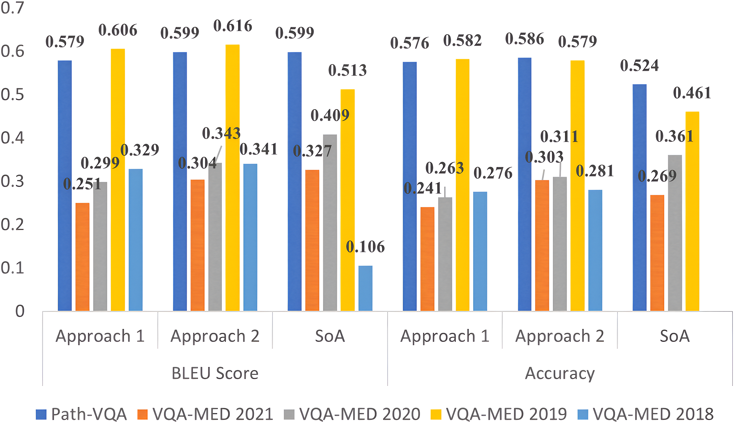
The results of the MVQA models generated from Approach 1 and Approach 2 are validated using quantitative metrics and compared with state-of-arts (SoA). The performance analysis using accuracy and BLEU score for all datasets are given in Table 4 for approach 1 and Table 5 for approach 2. In these tables, SoA1, SoA2, SoA3, SoA4 and SoA5 represent Peng, Liu & Rosen (2018), Khare et al. (2021), Joshi, Mitra & Bose (2023), Gong et al. (2021) and Naseem, Khushi & Kim (2022) respectively. These two approaches are compared for all improved datasets in Fig. 2 for better understanding. From Table 4, it is observed that the improved VQA-MED 2019 and Path-VQA datasets attained 12.1% and 2.6% increased accuracy than SoA2 and SoA5 respectively. Because the VQA-MED 2019 dataset takes differentially weighting to each part of the sample images and in Path-VQA dataset, most of the labels have more than one sample hence performance is maintained. In terms of BLEU score, the VQA-MED 2018 and 2019 datasets achieved 22.3% and 9.3% increased BLEU score than SoA1 and SoA2 respectively. Because the VQA-MED 2018 dataset maintained the least sample to label ratio. The overall inference from Table 4 is that the accuracy and BLEU score are improved from 1.5% to 11.5% and 0.7% to 12.4% respectively for improved datasets.
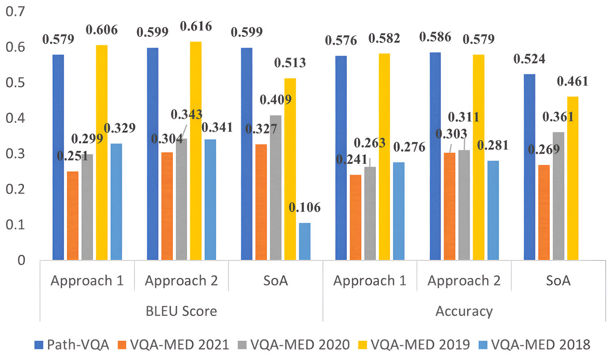
Figure 2: Performance analysis of MVQA datasets using quantitative metrics.
From Table 5, it is inferred that the VQA-MED 2018, VQA-MED 2019, and Path-VQA datasets perform better than SoA1, SoA2, and SoA5 by 23.5%, 11.8%, and 3.4%, respectively, when using Approach 2 in terms of BLEU score. Overall, the performance improvement ranges from 3% to 12.6% in accuracy and from 1.3% to 11.0% in BLEU score for the improved datasets. This demonstrates that normalization through mathematical computation helps standardize the datasets and supports the generation of more effective models by augmenting underrepresented samples. Figure 2 shows that Approach 2 (ResNet followed by LSTM) outperforms Approach 1 (VGGNet followed by LSTM). Approach 2 is also visualized using XAI, which highlights the most significant information in the input data.
To assess the robustness of the observed performance improvements, statistical significance testing using a paired t-test between models trained on the original and augmented datasets are conducted. The results indicate that the improvements in both accuracy and BLEU score are statistically significant across all datasets, with p-values <0.05. In addition, we report 95% confidence intervals for each metric, calculated over five independent training runs with different random seeds. These intervals demonstrate consistent gains and minimal variance, further confirming the reliability of the proposed augmentation techniques. Detailed results, including mean standard deviation and p-values, are given in Table 6.
| Dataset | Model | Accuracy (%) | 95% CI (Acc) | BLEU score | p-value |
|---|---|---|---|---|---|
| D1 | Original | 0.167 ± 0.09 | [0.158–0.176] | 0.231 ± 0.02 | − |
| Augmented | 0.281 ± 0.06 | [0.275–0.287] | 0.341 ± 0.01 | <0.01 | |
| D2 | Original | 0.491 ± 0.012 | [0.480–0.503] | 0.561 ± 0.03 | − |
| Augmented | 0.579 ± 0.08 | [0.571–0.587] | 0.616 ± 0.02 | <0.05 | |
| D3 | Original | 0.282 ± 0.1 | [0.272–0.292] | 0.330 ± 0.02 | − |
| Augmented | 0.312 ± 0.09 | [0.303–0.321] | 0.343 ± 0.01 | <0.01 | |
| D4 | Original | 0.218 ± 0.1 | [0.208–0.228] | 0.254 ± 0.02 | − |
| Augmented | 0.303 ± 0.09 | [0.294–0.312] | 0.304 ± 0.01 | <0.01 | |
| D5 | Original | 0.460 ± 0.1 | [0.450–0.470] | 0.565 ± 0.02 | − |
| Augmented | 0.586 ± 0.09 | [0.577–0.595] | 0.595 ± 0.01 | <0.01 |
Analysis of visual representation using XAI
The most significant region in the image and question, which contributes for answer prediction are highlighted using XAI techniques and it is shown in Figs. 3, 4, 5, 6 and 7. From Figs. 3, 4 and 5, the MVQA datasets are analysed under different perspectives namely, (i) Visualization of one image with multiple QA pairs (ii) Visualization of one QA pair with multiple images (iii) Visualizing the QA pair for the sample from original and improved dataset. Since Path-VQA dataset are less complex, VQA-MED 2021 dataset are analysed by visualizing different abnormalities of same body region and it is shown in Fig. 6. The VQA-MED 2021 dataset is chosen because it consists of abnormality related questions which are difficult to answer as compared with other types. Among the images, the samples related to abnormality on and around the knee joint are considered for understanding the disparity among similar type medical images. Finally, the limitations with respect to each MVQA dataset is shown in Fig. 7.
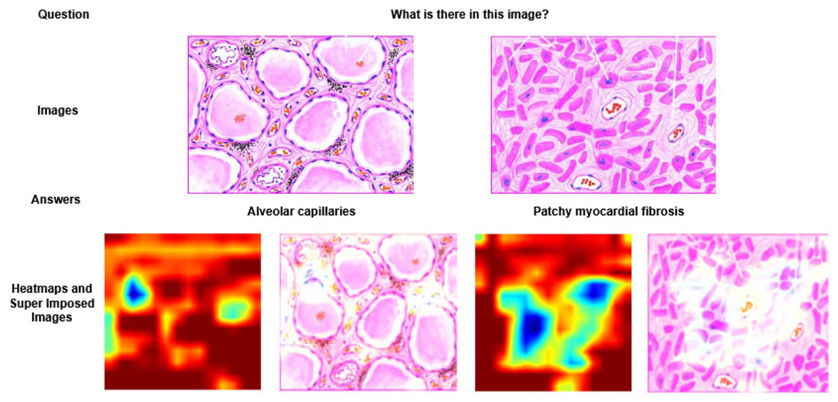
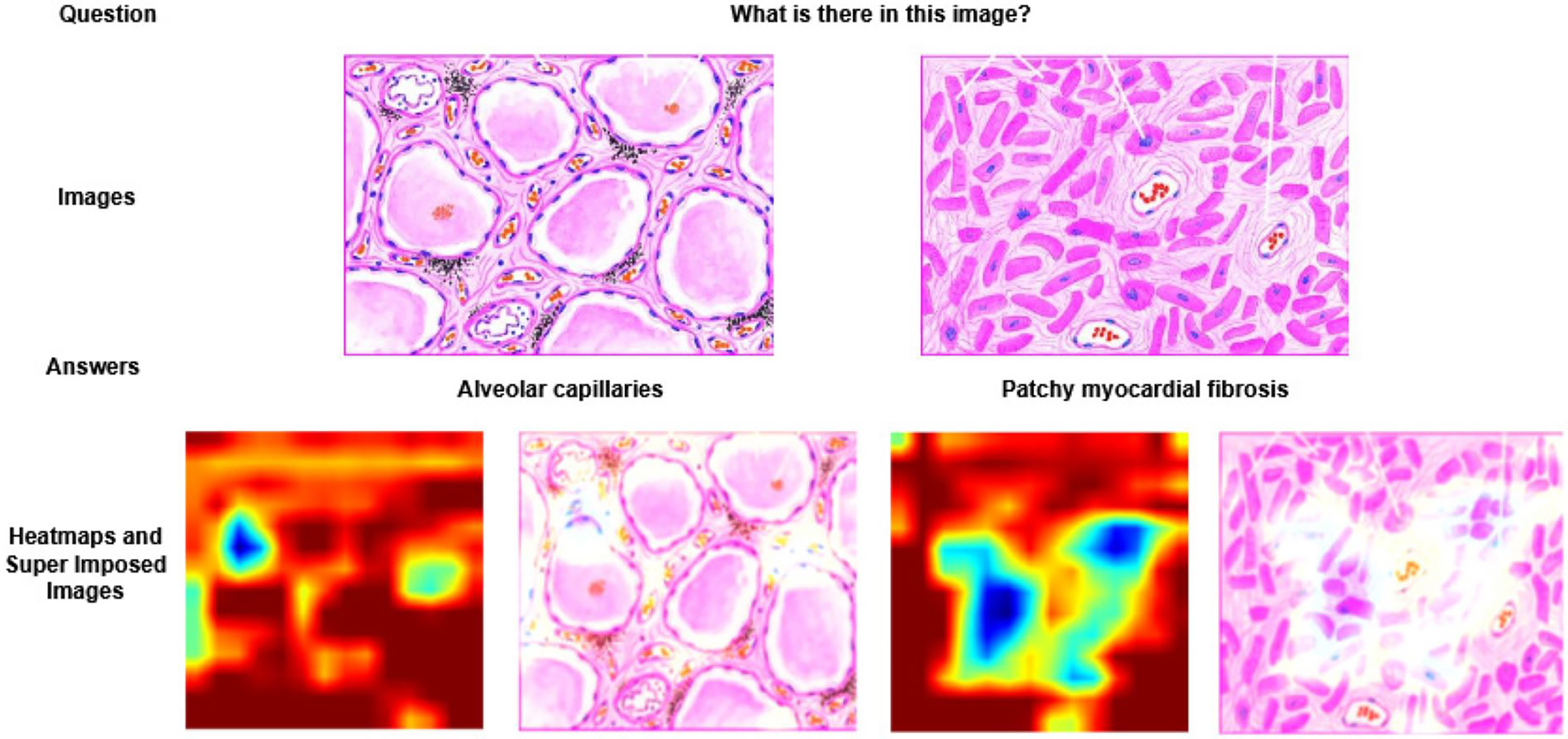
Figure 3: Visualization of heatmaps and super imposed images for different samples.
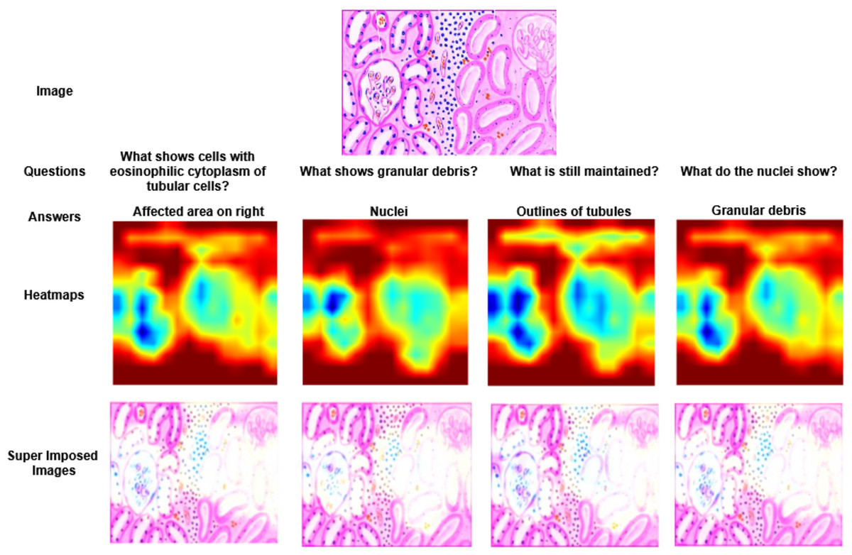
Figure 4: Visualization of heatmaps and their superimposed images for four different Question–Answer (QA) pairs.
The heatmaps highlight the image regions most relevant to each question, illustrating how the model focuses on contextually significant areas while generating responses.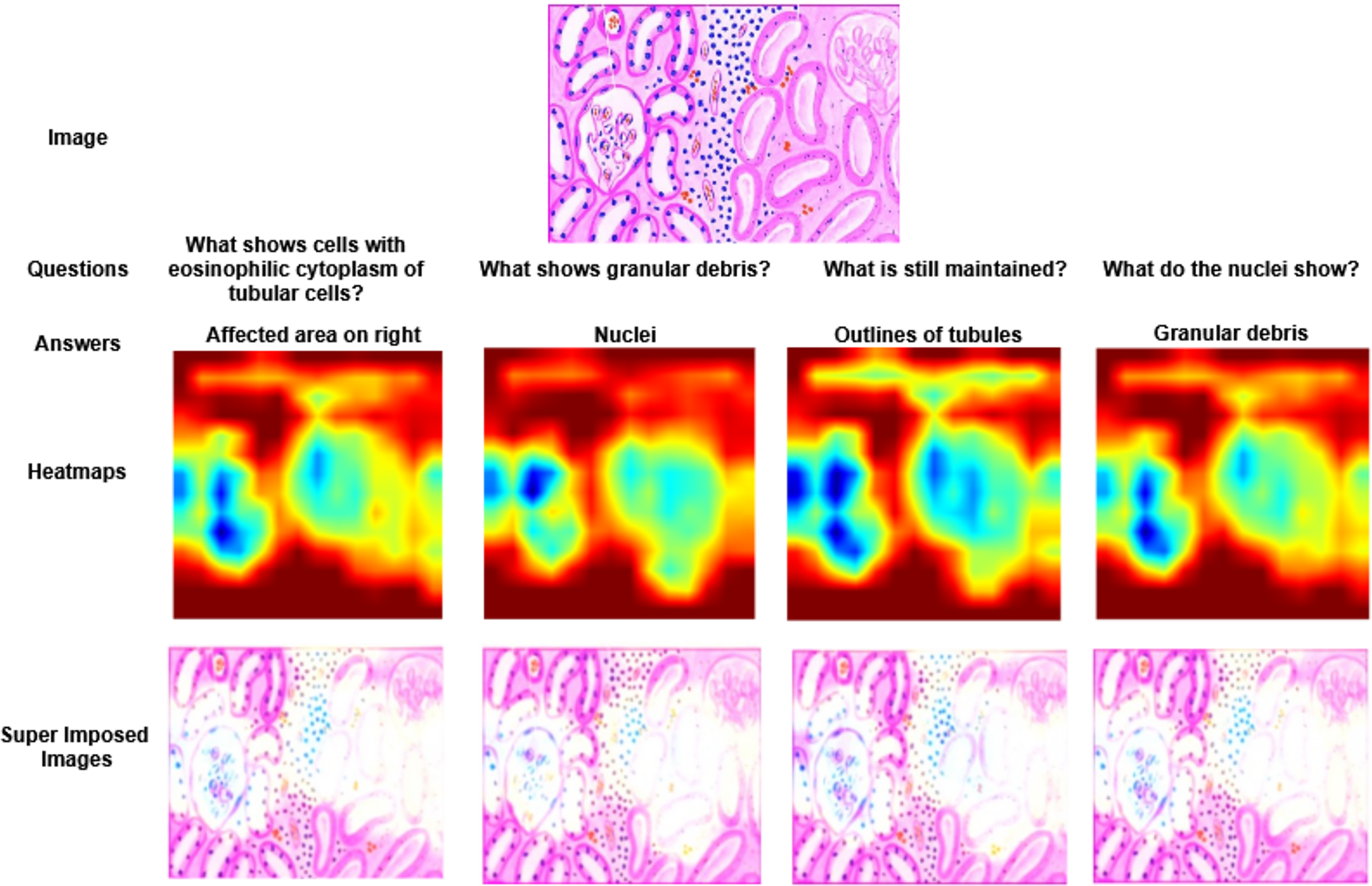
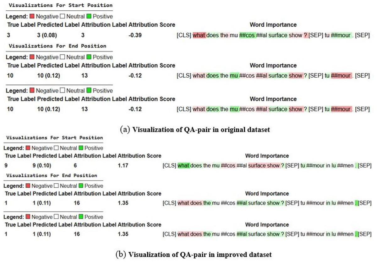
Figure 5: Visualization of question–answer (QA) pairs from the original and improved Path-VQA datasets.
The comparison illustrates enhancements in dataset quality, clarity, and relevance, highlighting how the improved dataset provides more accurate and contextually aligned QA pairs.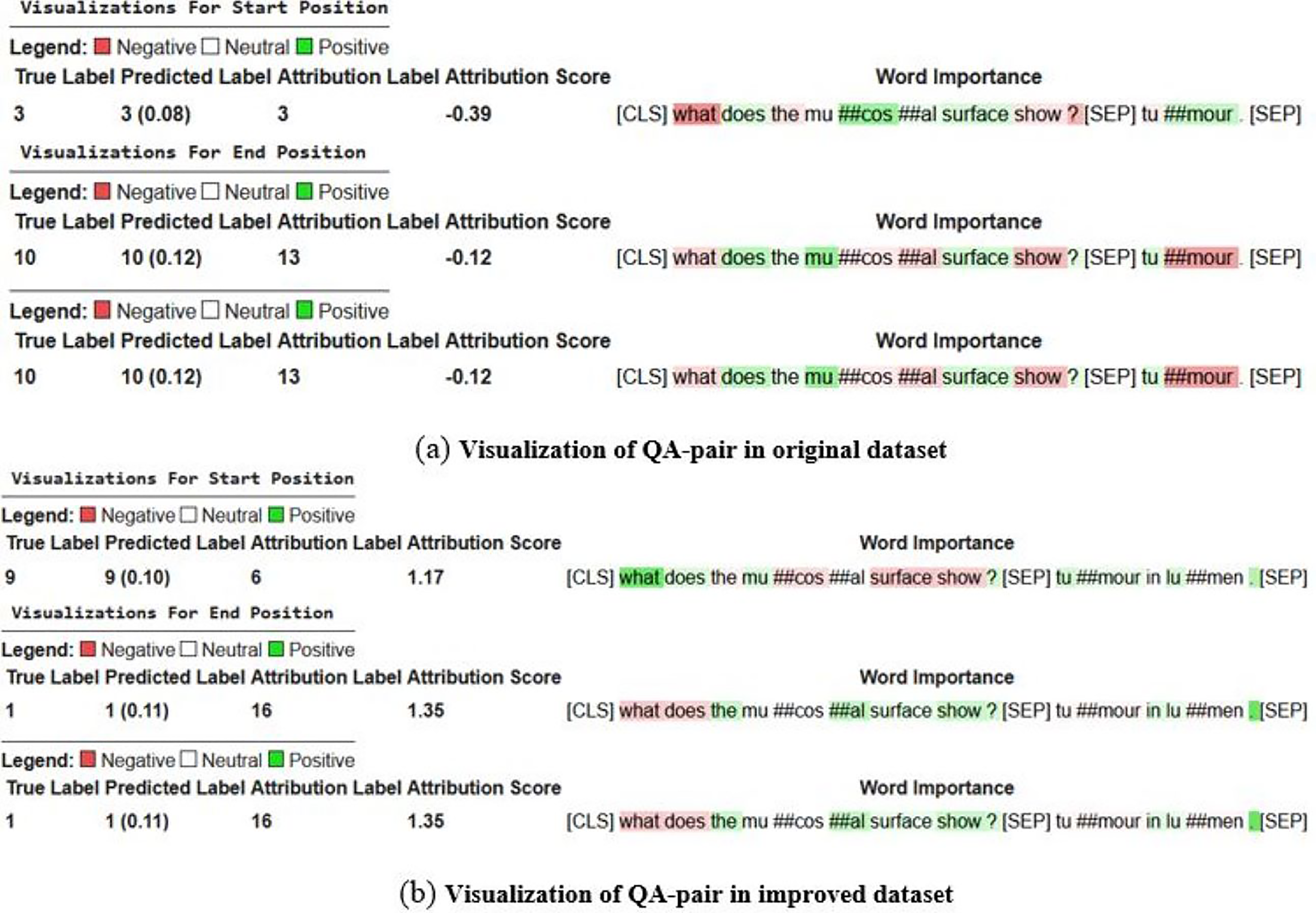
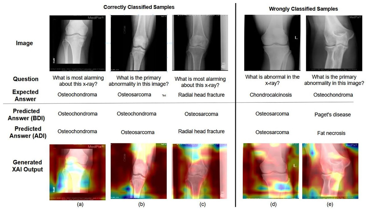
Figure 6: Examples of correctly and incorrectly predicted samples from the VQA-MED 2021 dataset.
The figure illustrates the model’s performance by showing cases where predictions align with ground truth answers and instances where errors occur, helping to analyze common success patterns and failure modes.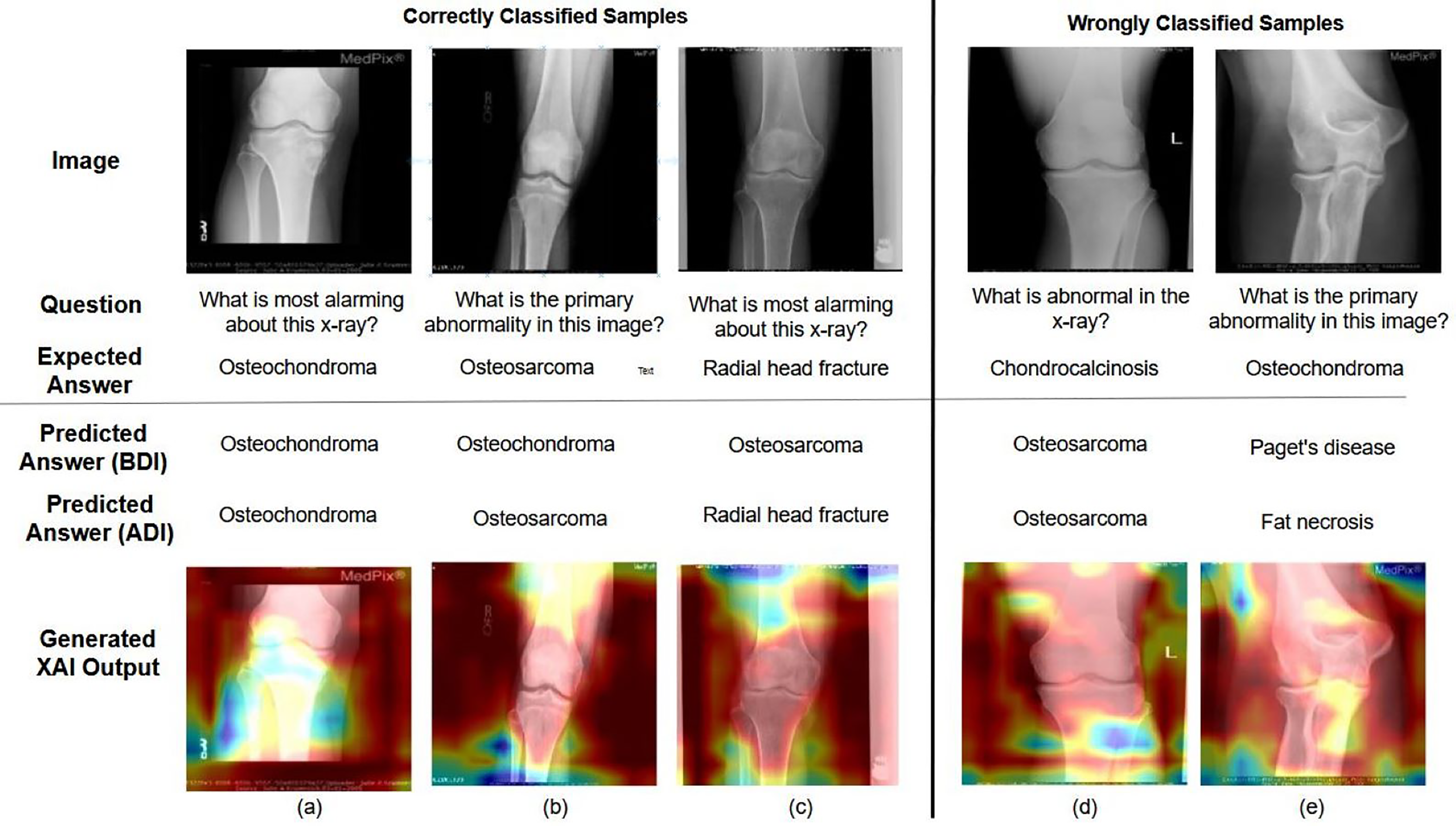
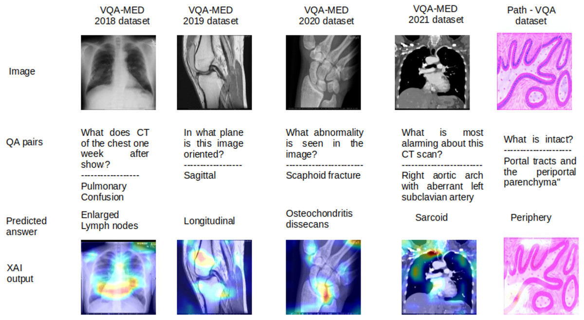
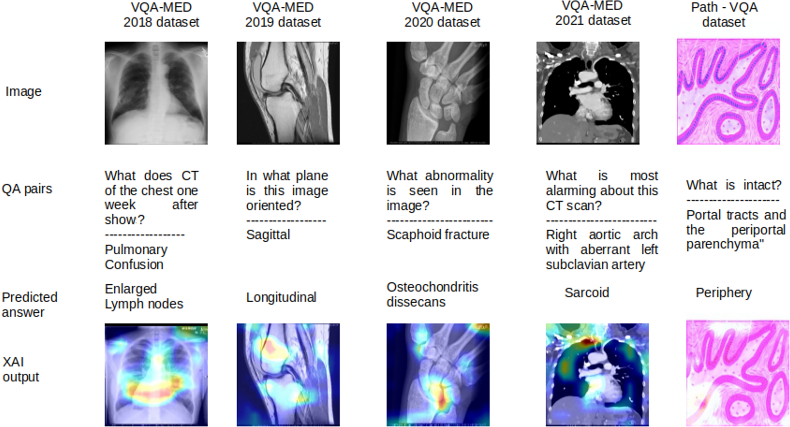
Figure 7: Limitations in MVQA datasets.
In Fig. 3, two different images of same question “What is there in the image?” are illustrated with answers, heatmaps and super imposed images. From the figure, it has been inferred that the generated heatmap varied by colour intensity, location and quantity of the image depending on the input and, as a result the respective super imposed image also varied accordingly. Similarly in Fig. 4, four different QA pairs for the answers “affected area on right”, “nuclei”, “outlines of tubules” and “granular debris” are illustrated for the same medical image. From the figure, it has been inferred that depending on the QA pairs of the same image, the respective heatmap varied because of the contribution of different regions in the image towards answer prediction and it is reflected in the generated super imposed image.
The XAI visualization and its analysis for QA pairs are shown in Fig. 5. In this figure, the answer to the question “What does the mucosal surface show?” is “tumour in lumen,” according to the dataset. The model trained on the original dataset predicts the answer as “tumour” (partially correct), whereas the model trained on the improved dataset correctly predicts “tumour in lumen.” In this figure, the context of the words is represented using three different colors: green (positive context), white (neutral context), and red (negative context). In Fig. 5B, the context of the keywords “does,” “mucosal,” and “surface” contributes to the answer prediction from different perspectives and is shown in green. However, in Fig. 5A, the context of the answer with respect to the question varies from positive to negative. So far, the importance of LRP XAI in interpreting pathology images and QA pairs has been demonstrated through these visualizations. The role of XAI in identifying the reasons behind misclassified samples is discussed in the following paragraph.
The MVQA (before and after improvement) outcome and LRP XAI output are shown to demonstrate the effect of augmentation and visualisation in answer prediction in Fig. 6. In Figs. 6A, 6B and 6C represents correctly classified samples, Figs. 6D and 6E represents wrongly classified samples. Among the correctly classified samples, the proposed MVQA model predict appropriate answer after dataset improvement that shows the effect of augmented datasets in developed MVQA model. In terms of visualization, LRP XAI highlights the region around the knee joint (a) “Osteochondroma” is an overgrowth of cartilage at the knee joint (b) “Osteosarcoma” is a bone cancer that is developed in the osteoblast cell and hence the long bone is highlighted (c) “Radial head fracture” occurs at the diverging line from the joint, so the region around radial head is highlighted. On the other hand, for (d) Instead of “Chondrocalcinosis” (Calcium pyrophosphate crystal deposits in the joint tissues), the model predicted the output as “Osteosarcoma” (e) Model predicted output as “fat necrosis” (death of fat tissues due to injury) instead of “Osteochondroma”. As per the visualization in both cases, instead of knee joint, the model learned the random features from surrounding bones and muscles. As per the visualization in both cases, instead of knee joint, the model learned the random features from surrounding bones and muscles. Moreover, the limitations corresponding to different MVQA datasets are also visualized using LRP XAI.
The limitations of all MVQA datasets are also analysed using LRP XAI are shown in Fig. 7 for some samples. In this figure, the output are shown in the order of the input images, question with actual answers (QA pairs), wrongly predicted answers and the output of LRP XAI visualization. Because these samples have more visualization effect with less deviation in interpretation for different organs, planes and modalities. For the sample of VQA-MED 2018 dataset, the proposed model captured the features from the lymph region instead of the lung and hence, the lymph node related abnormality is generated and it is visualized in LRP XAI output. In the case of VQA-MED 2019 dataset, the region in the patellofemoral bone is identified but the plane type is varied from sagittal to longitudinal because these two plane types are slightly varied from each other. In the VQA-MED 2020 dataset, the proposed model considers the Phalanges aspatellofemoral bone and hence predicted output as osteochondritis dissecans. For the VQA-MED 2021 dataset, the answer is predicted based on the growth of inflammatory cells because of the synonyms used in the question. In Path-VQA dataset, the tissue is damaged between portal tract and periportal parenchyma but the model captured the region at the outer layer and hence output as peripheral.
Conclusion and future work
The proposed work focuses on three key perspectives, namely: (i) the creation of the Path-VQA dataset, (ii) augmentation of existing MVQA datasets to improve model performance, and (iii) validation of results using quantitative metrics and the LRP XAI technique. The Path-VQA dataset was developed using images from pathology textbooks, aligned with corresponding QA pairs, and validated by a medical expert. The four VQA-MED datasets, along with the Path-VQA dataset, were augmented using mathematical transformations, Mixup strategies, and label smoothing techniques. These enhanced datasets were then used to train improved MVQA models, whose performance was evaluated using standard quantitative metrics and the LRP XAI approach.
The analysis revealed that the improved Path-VQA dataset achieved 6.2% higher accuracy than the state-of-the-art model (Faster Region based Convolution Neural Network with Gated Recurrent Unit (GRU)), particularly when using a ResNet and LSTM-based architecture. Similarly, all enhanced MVQA datasets outperformed their original versions, with accuracy improvements ranging from 3% to 12.6% and BLEU score gains between 1.3% and 11.0%. The LRP XAI technique further supported the model’s predictions by highlighting relevant regions in both images and textual questions, thereby improving the transparency and trustworthiness of the outputs. This interpretability is especially valuable in the medical domain, as it: (i) enables differentiation between closely related disorders by emphasizing relevant image regions, (ii) helps non-experts understand complex medical content, and (iii) supports medical education by illustrating key concepts in context.
While the proposed system makes notable improvement in mitigating dataset scarcity and improving interpretability, it still faces several limitations. Current datasets may not fully capture the diversity and granularity required to detect subtle abnormalities such as occult stress fractures, micro-cracks in bones, or minor soft tissue tears. Additionally, potential biases may persist due to the limited source variety in training data, which could affect generalizability across broader patient populations. Furthermore, while LRP offers valuable insights, relying on a single XAI technique may not provide a complete explanation of model behavior.
Future work should therefore focus on: (i) incorporating more diverse and clinically representative datasets, including annotated medical reports and prescriptions, to broaden the system’s QA capabilities; (ii) addressing dataset and model biases through robust validation across different patient populations; and (iii) exploring alternative XAI methods to visualize and cross-validate explanations from multiple interpretability perspectives. Ultimately, the goal is to develop a real-time, deployable tool—such as a mobile or web-based application—that can assist clinicians, medical students, and the general public in understanding medical images and reasoning about clinical scenarios with greater reliability and clarity.