
Optimized Gaussian naïve Bayes for prostate cancer detection in White patients using gene expression data
- Published
- Accepted
- Received
- Academic Editor
- Consolato Sergi
- Subject Areas
- Bioinformatics, Computational Biology, Algorithms and Analysis of Algorithms, Artificial Intelligence, Data Mining and Machine Learning
- Keywords
- Gaussian naïve Bayes, Gene expression data, Machine learning, Bioinformatics, Computational biology, Artificial intelligence, Prostate cancer
- Copyright
- © 2025 Agustriawan et al.
- Licence
- This is an open access article distributed under the terms of the Creative Commons Attribution License, which permits unrestricted use, distribution, reproduction and adaptation in any medium and for any purpose provided that it is properly attributed. For attribution, the original author(s), title, publication source (PeerJ Computer Science) and either DOI or URL of the article must be cited.
- Cite this article
- 2025. Optimized Gaussian naïve Bayes for prostate cancer detection in White patients using gene expression data. PeerJ Computer Science 11:e3405 https://doi.org/10.7717/peerj-cs.3405
Abstract
Background
Prostate cancer remains a major health concern worldwide. Racial disparities in prostate cancer diagnosis underscore the need for diagnostic approaches to manage the disease across different racial groups. Machine learning techniques, particularly Gaussian naïve Bayes, offers a promising method to improve diagnostic accuracy by identifying complex patterns in gene expression data. Gaussian naïve Bayes performs well with small datasets, minimizing the risk of overfitting.
Method
Gene expression and phenotype datasets were retrieved from the University of California, Santa Cruz (UCSC) Xenabrowser. Differentially expressed gene (DEG) analysis and receiver operating characteristic (ROC) evaluation were performed for race-specific populations. The resulting features were incorporated into multiple scenarios to develop machine learning models, combining feature selection, balancing techniques, and hyperparameter tuning within the Gaussian naïve Bayes algorithm to optimize prostate cancer diagnosis. Furthermore, Local Interpretable Model-Agnostic Explanations (LIME) was employed to interpret the impact of the selected features.
Results
The study evaluated 96 scenarios involving combinations of 4, 7, 13, and 139 gene features with balancing techniques and hyperparameter tuning to build machine learning models using the Gaussian naïve Bayes algorithm for prostate cancer detection. The highest accuracy for White race samples was achieved with 13 genes, resulting in 95% accuracy. LIME analysis identified the gene features with the greatest influence on model predictions. The model was further validated on Black race samples, achieving an accuracy of 93%.
Conclusion
The study demonstrates that Gaussian naïve Bayes, when combined with race-specific feature selection and hyperparameter tuning, can detect prostate cancer with high accuracy. These findings highlight the potential of Gaussian naïve Bayes for addressing prostate cancer detection in race-specific populations.
Introduction
Prostate cancer remains a leading cause of cancer-related mortality worldwide. In a large cohort study, 752,352 patients with prostate cancer were identified, of whom 180,862 (24.0%) died during follow-up (Hinata & Fujisawa, 2022; Lowder et al., 2022; Porcacchia et al., 2022). This 24% mortality rate underscores the critical importance of early detection to mitigate substantial health risks. Machine learning (ML) techniques have emerged as powerful tools for predicting prostate cancer with superior accuracy (Chen et al., 2022; Yaqoob, Musheer Aziz & Verma, 2023). Consequently, ML gained importance in the health sector as promising diagnostic approach, capable of identifying intricate patterns in complex datasets and, effectively predicting cancer outcomes (Kourou et al., 2015).
The Gaussian naïve Bayes algorithm, a probabilistic classifier based on Bayes’ theorem, offers rapid computational efficiency and excels at handling continuous numerical data (Anand et al., 2022; Kamel, Abdulah & Al-Tuwaijari, 2019; Gayathri & Sumathi, 2016). It simplifies computations, making it particularly efficient for high-dimensional datasets (Salmi & Rustam, 2019). These characteristics make Gaussian naïve Bayes well-suited for analyses involving small sample sizes and large gene sets, as commonly encountered in prostate cancer research. Additionally, hyperparameter tuning can significantly enhance its performance (Rahman et al., 2023; Yanuar, Sa’adah & Yunanto, 2023). However, while ML models like Gaussian naïve Bayes can improve diagnostic accuracy, prostate cancer outcomes are also influenced by key factors such as racial disparities (Burnett, Nyame & Mitchell, 2023; Lillard et al., 2022).
Racial disparities represent a critical challenge in prostate cancer management. African American men, for instance, are 76% more likely to be diagnosed with prostate cancer and face a 1.2-fold higher mortality rate compared to White men. Conversely, Asian American men are 55% less likely to receive a diagnosis than White men (Hansen et al., 2022). These variations in survival outcomes across racial groups necessitate race-specific analyses to improve detection and treatment strategies. Addressing racial disparities in prostate cancer diagnosis is essential for improving overall outcomes.
Gene expression studies have proven invaluable for identifying biological pathways and understanding the mechanisms of complex diseases. By analyzing these data through functional pathway approaches, researchers can strengthen mechanistic insights and discoveries (Ramanan et al., 2012). This highlights the substantial potential of genomic data in medicine particularly for cancer detection (Ding et al., 2010; Guan et al., 2012). Differentially expressed gene (DEG) analysis enables the identification of distinct gene expression patterns, with well-known algorithms including DESeq2, edgeR, and limma (Mohammad et al., 2022; Rosati et al., 2024). When integrated with ML, this framework can uncover genetic markers that may account for racial disparities in prostate cancer diagnosis.
Despite advances in prostate cancer detection using Gaussian naïve Bayes with gene expression data, racial disparities have not been sufficiently addressed as a primary risk factor. Prior research has demonstrated the efficacy of naïve Bayes in prostate cancer detection. For example, one study analyzed a dataset of 12,533 genes from 102 samples, applying sequential forward feature selection (SFFS) to identify 21 key genes. Among ML methods tested, including artificial neural networks (ANNs), naïve Bayes, and J48, naïve Bayes achieved 86.27% accuracy in detecting prostate cancer (Tirumala & Narayanan, 2019). Another investigation using 489 samples and feature selection via MATLAB’s Classification Learner toolbox (though without specifying the final gene set), reported up to 67% accuracy with naïve Bayes (Antunes et al., 2025). In comparison, a separate study with 43,497 features employed Weka tool for feature selection was performed using the Weka data mining tool and achieved 95.8% accuracy using support vector machine (SVM) on six transcripts highlighting the potential for high performance in gene-based models (Alkhateeb et al., 2019). Notably, these studies overlook racial factor in gene selection for ML modeling.
To bridge this gap, the present study proposes a race-specific ML approach for prostate cancer diagnosis using an incorporating optimized feature selection and the Gaussian naïve Bayes algorithm. Lastly, the model will be interpreted using Local Interpretable Model-agnostic Explanations (LIME) and validated on a Black race dataset to evaluate its generalizability.
Methods
The workflow of this study is illustrated in Fig. 1. The method encompasses several key steps, including data gathering, data preprocessing, feature selection and ML modeling. All analyses were conducted using Python version 3.13.2 in Visual Studio Code environment. The computational setup included a Windows 11 operating system, an Intel Core i5 processor, 16 GB of RAM, and a 512 GB SSD, ensuring efficient data processing and model training.
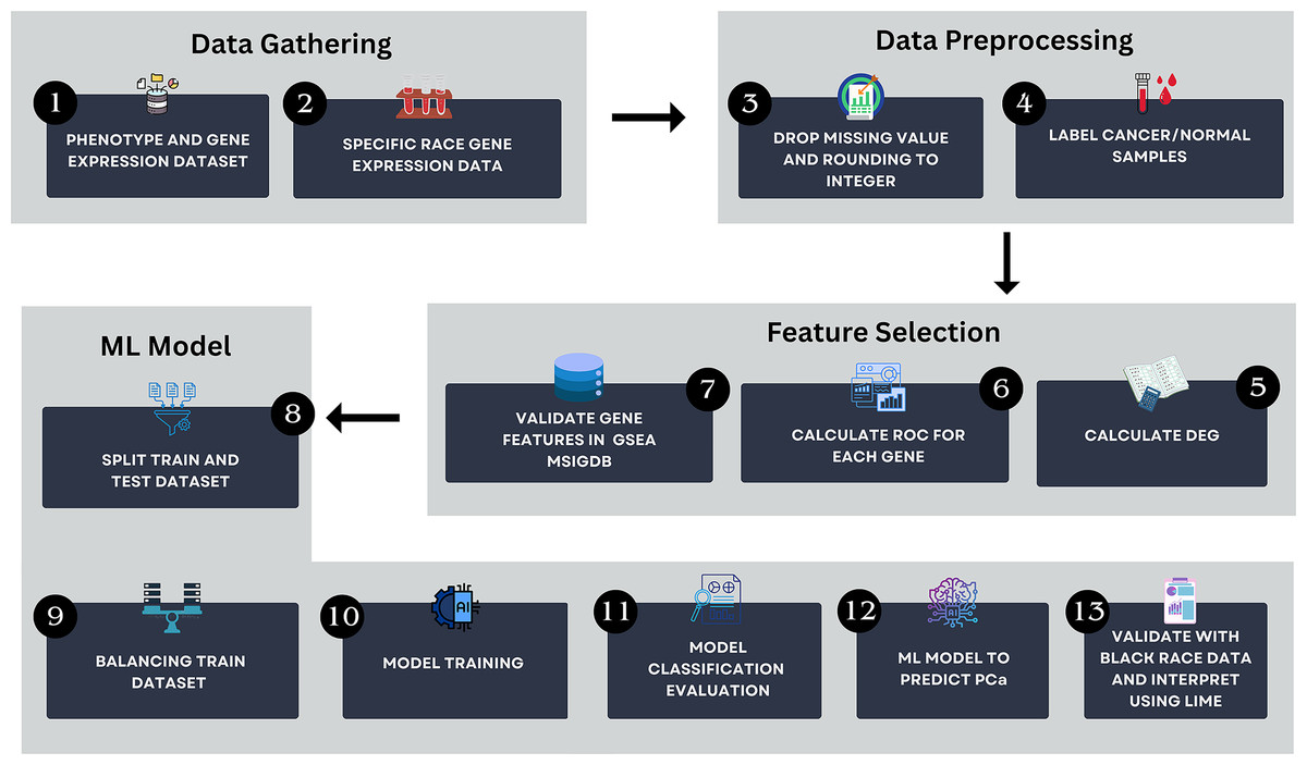
Figure 1: The research pipeline which consists of key steps such as data gathering, data preprocessing, feature selection, and AI modeling.
This pipeline outlines the detailed process followed in this study to develop the model.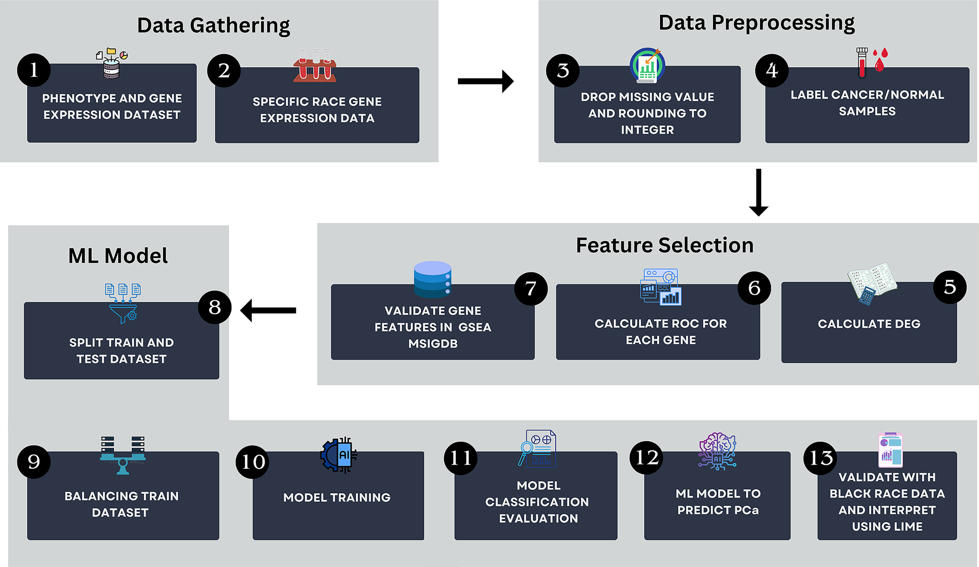
Data gathering
This study utilized a dataset comprising gene expression and phenotype data for prostate cancer. The HTSeq—Counts gene expression and GDC TCGA-PRAD phenotype data were retrieved on August 25, 2024, from the UCSC Xena browser—(https://xenabrowser.net/) (Goldman et al., 2020). The dataset had been pre-normalized using log2(count+1) transformation to ensure the values were on a comparable scale.
Data preprocessing
During preprocessing, the gene expression and phenotype datasets were stratified by race. Python packages pandas (version 2.2.2) and NumPy (version 1.26.4) were employed to remove rows with missing values and to round the data from floating-point to integer types. Then, the processed dataset was labeled as “cancer” and “normal” using scikit-learn (version 1.5.1).
Feature selection
DEG analysis was conducted on the labeled data using the PyDESeq2 library (version 0.4.10). PyDESeq2 was chosen for its robustness in identifying differentially expressed genes through effective statistical methods. The DEG results served as features for ML model development. Features were selected based on specific thresholds, as outlined in Table 1. Each parameter plays a distinct role in feature selection: basemean represents the average normalized expression level, log2FoldChange determines upregulated and downregulated genes, and padj identifies statistically significant genes (Love, Huber & Anders, 2014). A positive log2 foldchange value indicates upregulated with higher expression, whereas a negative value indicates downregulated genes with lower expression. This metric is essential for highlighting biologically relevant changes in gene expression. The log2FoldChange thresholds (0.35 and 0.4) were selected to investigate their impact on model performance and are commonly applied in DEG studies to capture biologically relevant expression variations.
| Scenario | Threshold criteria |
|---|---|
| 1 | Baseman >= 10 and padj < 0.05 |
| 2 | Basemean >= 10, padj < 0.05 and log2foldchange < 0.35 |
| 3 | Basemean >= 10, padj < 0.05 and log2foldchange < 0.4 |
| 4 | Basemean >= 10, padj < 0.05 and ROC > 0.9 |
Moreover, receiver operating characteristic (ROC) analysis was performed to identify potential biomarker genes. An area under the curve (AUC-ROC) value closer to 1 indicates superior discrimination, with high true-positive sensitivity and low false-positive rates (Hajian-Tilaki, 2013). This study applied an AUC-ROC threshold greater than 0.9, indicating excellent discriminatory power (Casarrubios et al., 2022; Unal, 2017). ROC visualizations were generated using Matplotlib (version 3.8.3). As gene identifiers were in Ensembl_ID, the SynGO website was used to convert them to gene name symbols (Koopmans et al., 2019). The selected genes were further verified via Gene Set Enrichment Analysis (GSEA) using the Molecular Signatures Database (MsigDB) to confirm their association with prostate cancer (Liberzon et al., 2015).
Gaussian naïve Bayes modeling with several scenarios
The dataset was divided into training and test sets using split ratios of 60/40, 70/30, and 80/20. Class imbalances were mitigated by applying balancing techniques to augment the minority class, achieving a 1:3 ratio. To maintain the natural distribution and ensure unbiased evaluation, balancing was applied solely to the training data; the test data remained unmodified. The balancing methods included Random Oversampling, KMeans SMOTE, Borderline SMOTE and SMOTEEN. SMOTE-based methods were prioritized for their ability to generate synthetic samples with high-dimensional genomic data. Adaptive Synthetic Sampling (ADASYN) was excluded, as it may over generate synthetic instances for noisy or ambiguous samples, potentially comprising classifier robustness in small biomedical datasets (Mitra, Bajpai & Biswas, 2023). Balancing was implemented using imbalanced-learn package (version 0.12.3). Models were further optimized through hyperparameter tuning.
This study explored multiple scenarios incorporating various feature selection methods, data split ratios, balancing techniques, and hyperparameters, detailed in Table 2, yielding a total of 96 scenarios.
| Feature selection | Splitting ratio | Balancing technique | Hyperparameter |
|---|---|---|---|
| DEG analysis with base mean >= 10, and padj < 0.05 | 80:20 70:30 60:40 | Random Oversampler SMOTEEN KMeans SMOTE Borderline SMOTE | Yes/No |
| DEG analysis with base mean >= 10, padj < 0.05 and log2foldchange < 0.35 | 80:20 70:30 60:40 | Random Oversampler SMOTEEN KMeans SMOTE Borderline SMOTE | Yes/No |
| DEG analysis with base mean >= 10, padj < 0.05 and log2foldchange < 0.4 | 80:20 70:30 60:40 | Random Oversampler SMOTEEN KMeans SMOTE Borderline SMOTE | Yes/No |
| DEG analysis with base mean >= 10, padj < 0.05 and ROC > 0.9 | 80:20 70:30 60:40 | Random Oversampler SMOTEEN KMeans SMOTE Borderline SMOTE | Yes/No |
Model evaluation
Model performance was evaluated through classification reports, encompassing metrics such as accuracy, precision, recall, and F1-scores. These metrics are crucial for evaluating the model harmonization between training and test data. Accuracy reflects the percentage of correctly classified samples (cancer or normal), precision measures the percentage of true positives among predicted positives, recall indicates the percentage of actual positive correctly identified; and the F1-score represents the harmonic mean of precision and recall (Miller et al., 2024). To assess overfitting or underfitting, performance metrics (accuracy, precision, recall and F1-score) were compared between training and test sets, with consistency suggesting strong generalization. Model evaluation was performed using scikit-learn (version 1.5.1). Following classification, the best-performing model was interpreted using LIME to identify the most influential genes contributing to individual predictions.
Black race validation
To evaluate the model’s generalizability across racial groups, validation was performed on the Black race dataset, which had been separated during initial preprocessing steps. The identical preprocessing pipeline was applied, including data transformation and feature selection using DESeq2 with the same thresholds. The model, trained on the White race dataset, was applied without retraining to classify the Black race test data, enabling a direct comparison of cross-racial performance.
Results
Dataset gathering
The dataset used in this study comprised HTSeq-Counts gene expression data and GDC TCGA-PRAD Phenotype data. The HTSeq—Counts dataset included 60,488 genes and 551 patient samples, while the GDC TCGA-PRAD Phenotypes dataset contained 172 medical record variables. This study focused on the White population for building the ML model for prostate cancer detection, as it constituted the majority of the dataset (approximately 83%, or 458 of 551), providing a robust foundation for training process. Additionally, the Black race subset was used to validate the model’s performance. The distribution of age and Gleason score for White patients is depicted in Fig. 2. The age distribution indicates that the majority of patients were around 62 years old, suggesting a predominance of older individuals in the White race cohort. Additionally, the Gleason score distribution shows that a score of 7.0 was the most prevalent. Normal Gleason score range between 2–5, whereas scores of 6–10 indicate abnormal prostate cancer cell; higher scores reflect greater cellular abnormality (Tagai et al., 2019). The corresponding distributions for Black patients are shown in Fig. 3.
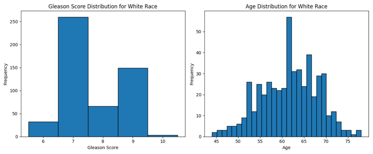
Figure 2: Age distribution and Gleason score for White race.
Graphs of age distribution and Gleason score on White patients. The age distribution indicates that most patients are between 60 and 65 years old. The Gleason score graph shows that a score of 7 is the most common, indicating abnormal prostate cancer cells.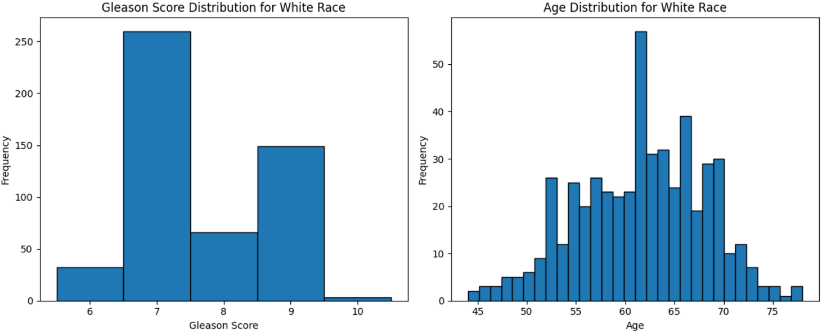
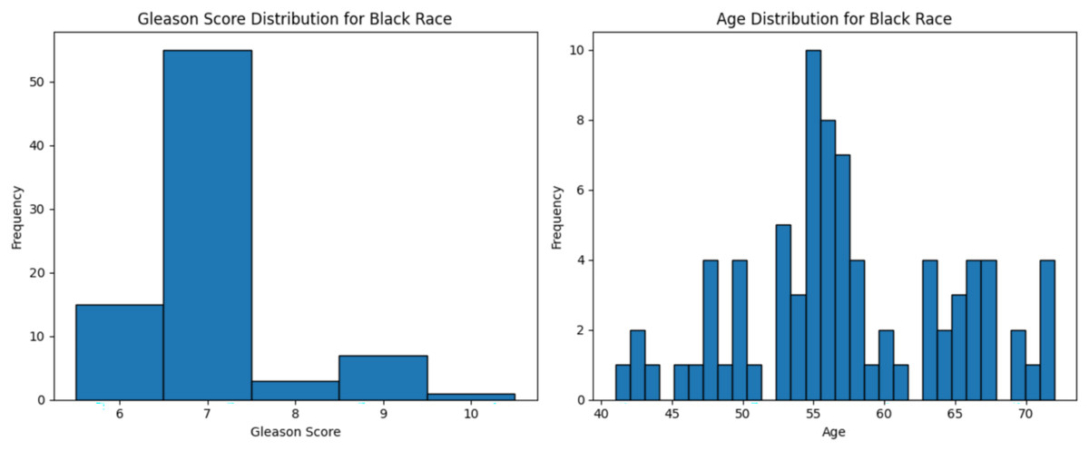
Figure 3: Age distribution and Gleason score for Black race.
Graphs of age distribution and Gleason score on Black patients. The age distribution indicates that most patients are between 60 and 65 years old. The Gleason score graph shows that a score of 7 is the most common, indicating abnormal prostate cancer cells.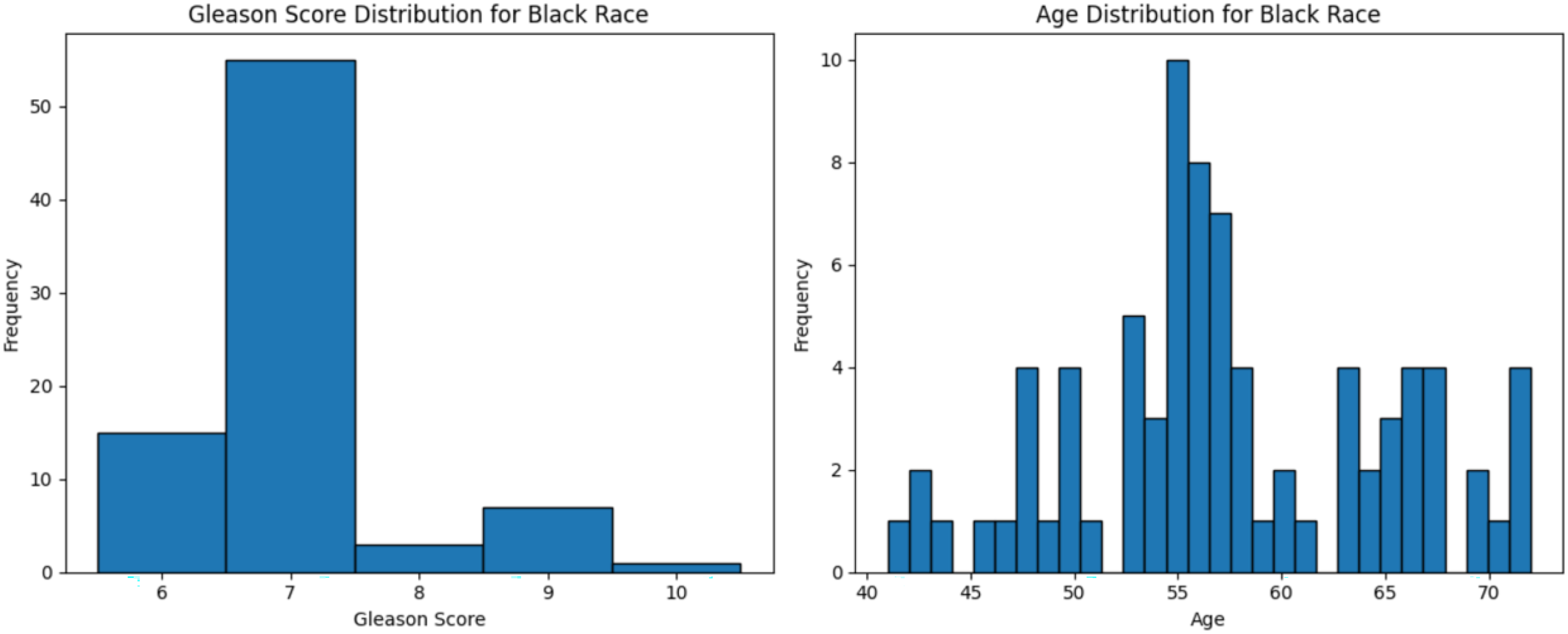
Data preprocessing
First, the data was cleaned by removing missing values and rounding the values into integers. As a result, the gene count was reduced from 60,488 to 57,429. Samples were then labeled as “cancer” or “normal” based on the TCGA barcode, where cancer is “01” denoted cancer and “11” indicated normal. The labeled samples were stored in a metadata for subsequent analyses, including feature selection, model training, and performance validation.
Feature selection
Four DEG analysis scenarios were conducted resulting 139, 7, 4 and 13 genes for scenario 1, 2, 3, and 4, respectively as detailed in Table 3.
| Scenario | Threshold criteria | Results (gene) |
|---|---|---|
| 1 | Baseman >= 10 and padj < 0.05 | 139 |
| 2 | Basemean >= 10, padj < 0.05 and log2foldchange < 0.35 | 7 |
| 3 | Basemean >= 10, padj < 0.05 and log2foldchange < 0.4 | 4 |
| 4 | Basemean >= 10, padj < 0.05 and ROC > 0.9 | 13 |
To refine scenario 1 further, the 139 genes were subjected to ROC analysis, resulting in a reduced set of 13 genes. The ROC analysis demonstrated high sensitivity for these 13 genes in detecting prostate cancer, as illustrated in Fig. 4.
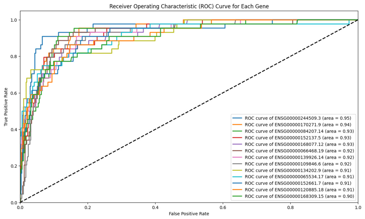
Figure 4: ROC analysis for 13 genes.
The ROC analysis for 139 genes, all of which have an AUC greater than 0.9. The high AUC scores indicate a strong sensitivity in distinguishing between the positive and negative classes.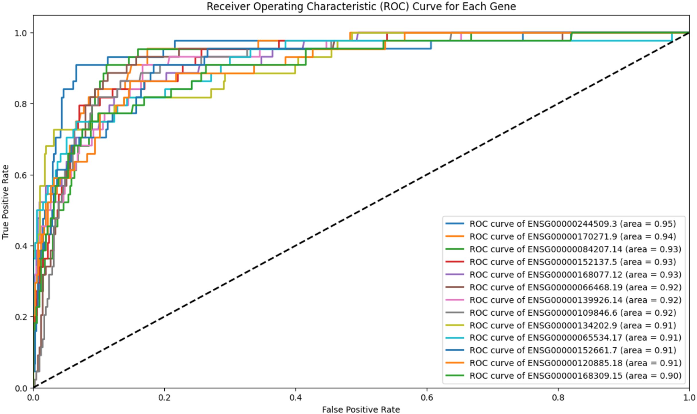
The Ensembl IDs of these 13 genes were converted to gene symbols and cross-referenced with MSigDB to assess their correlation with prostate cancer. According to MSigDB, nine out of the 13 genes, including GJA1, CLU, HSPB8, MYLK, CRYAB, FGFR2, GSTM3, GSTP1, and FRMD6, exhibited association with prostate cancer, as shown in Fig. 5. These genes suggest involvement in cancer-related pathways. The remaining genes (FAM107A, FAXDC2, SCARA3 and APOBEC3C) showed no direct correlation with prostate cancer. Despite this, these four genes were retained due to their strong predictive performance in ROC analysis, with AUC-ROC scores exceeding 0.9, indicating excellent discriminatory ability between cancer and non-cancer cases.
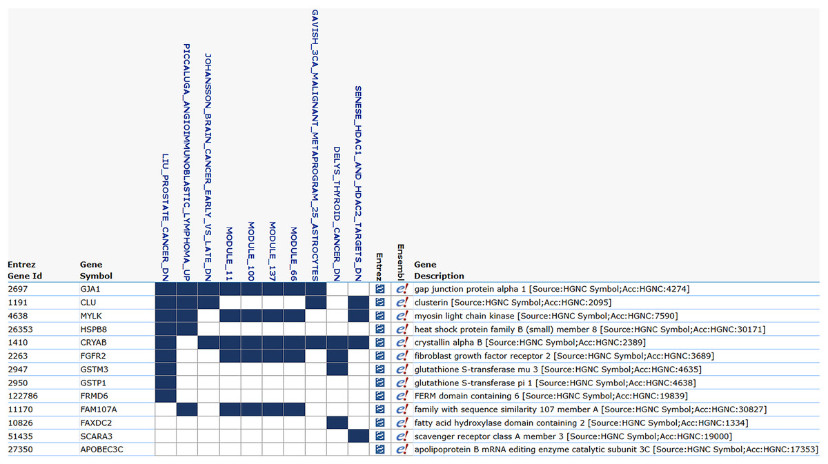
Figure 5: MSigDB prostate cancer correlation.
The correlation between gene features and prostate cancer. Nine genes are correlated with prostate cancer, and certain modules, such as module_11, module_66, and module_100, also exhibit a correlation with cancer.
Gaussian naïve Bayes Modeling
The gene sets from each scenario were processed using various splitting ratios and balancing techniques. The result for all modeling scenarios are presented in Tables 4–7.
| Number of gene | Splitting | Balancing technique | Hyperp-arameter tuning | Train accuracy | Test accuracy | Test precision | Test recall | Test F1-score |
|---|---|---|---|---|---|---|---|---|
| 4 | 60/40 | RandomOversampler | No | 89% | White race: 92% | White cancer: 95% | White cancer: 96% | White cancer: 95% |
| Black race: 93% | Black cancer: 96% | Black cancer: 96% | Black cancer: 96% | |||||
| 4 | 60/40 | RandomOversampler | Yes | 89% | White race: 92% | White cancer: 95% | White cancer: 96% | White cancer: 95% |
| Black race: 93% | Black cancer: 96% | Black cancer: 96% | Black cancer: 96% | |||||
| 4 | 60/40 | KMeansSMOTE | No | 95% | White race: 91% | White cancer: 93% | White cancer: 96% | White cancer: 95% |
| Black race: 93% | Black cancer: 95% | Black cancer: 97% | Black cancer: 96% | |||||
| 4 | 60/40 | KMeansSmote | Yes | 95% | White race: 91% | White cancer: 93% | White cancer: 96% | White cancer: 95% |
| Black race: 93% | Black cancer: 95% | Black cancer: 97% | Black cancer: 96% | |||||
| 4 | 70/30 | KMeansSMOTE | Yes | 95% | White race: 91% | White cancer: 93% | White cancer: 97% | White cancer: 95% |
| Black race: 93% | Black cancer: 95% | Black cancer: 97% | Black cancer: 96% |
| Number of gene | Splitting | Balancing technique | Hyperp-arameter tuning | Train accuracy | Test accuracy | Test precision | Test recall | Test F1-score |
|---|---|---|---|---|---|---|---|---|
| 13 | 70/30 | KMeansSMOTE | Yes | 93% | White race: 95% | White cancer: 97% | White cancer: 97% | White cancer: 97% |
| Black race: 93% | Black cancer: 98% | Black cancer: 93% | Black cancer: 96% | |||||
| 13 | 70/30 | KMeansSMOTE | No | 93% | White race: 95% | White cancer: 97% | White cancer: 97% | White cancer: 97% |
| Black race: 93% | Black cancer: 98% | Black cancer: 93% | Black cancer: 96% | |||||
| 13 | 80/20 | SMOTEEN | Yes | 95% | White race: 92% | White cancer: 97% | White cancer: 94% | White cancer: 96% |
| Black race: 90% | Black cancer: 99% | Black cancer: 90% | Black cancer: 94% | |||||
| 13 | 80/20 | SMOTEEN | No | 92% | White race: 92% | White cancer: 97% | White cancer: 94% | White cancer: 96% |
| Black race: 90% | Black cancer: 99% | Black cancer: 90% | Black cancer: 94% | |||||
| 13 | 80/20 | KMeansSMOTE | No | 92% | White race: 92% | White cancer: 97% | White cancer: 94% | White cancer: 96% |
| Black race: 90% | Black cancer: 99% | Black cancer: 90% | Black cancer: 94% | |||||
| 13 | 70/30 | No balancing | No | 90% | White race: 93% | White race: 98% | White race: 93% | White race: 96% |
| Black race: 85% | Black race: 83% | Black race: 100% | Black race: 91% |
| Number of gene | Splitting | Balancing technique | Hyperp-arameter tuning | Train accuracy | Test accuracy | Test precision | Test recall | Test F1-score |
|---|---|---|---|---|---|---|---|---|
| 139 | 70/30 | RandomOversampler | Yes | 91% | White race: 94% | White cancer: 98% | White cancer: 95% | White cancer: 97% |
| Black race: 93% | Black cancer: 98% | Black cancer: 93% | Black cancer: 96% | |||||
| 139 | 70/30 | RandomOversampler | No | 91% | White race: 94% | White cancer: 98% | White cancer: 95% | White cancer: 97% |
| Black race: 93% | Black cancer: 98% | Black cancer: 93% | Black cancer: 96% | |||||
| 139 | 60/40 | RandomOversampler | No | 93% | White race: 94% | White cancer: 99% | White cancer: 94% | White cancer: 97% |
| Black race: 95% | Black cancer: 99% | Black cancer: 95% | Black cancer: 97% | |||||
| 139 | 60/40 | RandomOversampler | Yes | 93% | White race: 94% | White cancer: 99% | White cancer: 94% | White cancer: 97% |
| Black race: 95% | Black cancer: 99% | Black cancer: 95% | Black cancer: 97% | |||||
| 139 | 80/20 | RandomOversampler | No | 94% | White race: 93% | White cancer: 96% | White cancer: 96% | White cancer: 96% |
| Black race: 94% | Black cancer: 98% | Black cancer: 95% | Black cancer: 97% |
| Number of gene | Splitting | Balancing technique | Hyperp-arameter tuning | Train accuracy | Test accuracy | Test precision | Test recall | Test F1-score |
|---|---|---|---|---|---|---|---|---|
| 7 | 80/20 | KMeansSMOTE | No | 94% | White race: 92% | White cancer: 95% | White cancer: 96% | White cancer: 96% |
| Black race: 93% | Black cancer: 95% | Black cancer: 97% | Black cancer: 96% | |||||
| 7 | 80/20 | KMeansSMOTE | Yes | 94% | White race: 92% | White cancer: 95% | White cancer: 96% | White cancer: 96% |
| Black race: 93% | Black cancer: 95% | Black cancer: 97% | Black cancer: 96% | |||||
| 7 | 70/30 | KMeansSMOTE | Yes | 95% | White race: 92% | White cancer: 95% | White cancer: 96% | White cancer: 95% |
| Black race: 93% | Black cancer: 96% | Black cancer: 97% | Black cancer: 96% | |||||
| 7 | 70/30 | KMeansSMOTE | No | 95% | White race: 92% | White cancer: 95% | White cancer: 96% | White cancer: 95% |
| Black race: 93% | Black cancer: 96% | Black cancer: 97% | Black cancer: 96% | |||||
| 7 | 60/40 | KMeansSMOTE | No | 95% | White race: 91% | White cancer: 95% | White cancer: 94% | White cancer: 95% |
| Black race: 93% | Black cancer: 96% | Black cancer: 96% | Black cancer: 96% |
As shown in Table 4, the optimal performance for prostate cancer detection was achieved with a 60/40 splitting ratio and the Random Oversampling, resulting a test accuracy of 92% for White patients and 93% for Black patients. This results also maintained high precision, recall, and F1-score values across both racial groups, reaching up to 96% for cancer classification. The effectiveness of only four features highlights the strength of the feature selection process, demonstrating that a minimal gene set can produce robust and reliable classification results. Furthermore, applying hyperparameter tuning did not significantly alter outcomes, indicating consistent model performance under default settings.
With 13 features (Table 5), the highest test accuracy of 95% for White patients and 93% for Black patients was attained using a 70/30 splitting ratio and KMeansSMOTE. This setup delivered consistent performance across metrics, with cancer detection scores up to 98%. Hyperparameter tuning had minimal impact, indicating the model’s robustness. Compared to other scenarios, this setup achieved a better balance between accuracy and generalizability across racial groups while utilizing a slightly larger feature set. The no-balancing scenario was only applied to the top performing datasets to ensure fair assessment without altering sample distributions. Accuracies without balancing were lower than those with balancing techniques, indicating that a moderate gene set, combined with suitable balancing and splitting, enhances accuracy and generalizability in race-aware prostate cancer classification models.
For 139 features (Table 6), the highest test accuracy of 94% with a 70/30 splitting ratio and Random Oversampling. This configuration consistently yielded strong cross-racial performance, with cancer detection metrics up to 99% in both groups. Random Oversampling proved most effective for this larger feature set, consistently appearing in top scenarios and providing stability.
Using seven features (Table 7), the model achieved its best test accuracy of 93% across racial groups with KMeansSMOTE. Performance was stable regardless of hyperparameter tuning or train-test split ratios (80/20, 70/30, and 60/40), with cancer metrics up to 97%. This highlights KMeansSMOTE’s reliability for smaller feature sets in race-specific cancer classification.
Among the 96 scenarios, the Gaussian naïve Bayes algorithm achieved its highest test accuracy of 95% for the White population and 93% for the Black population using 13 genes, a 70/30 split, the KMeansSMOTE, and hyperparameter tuning. This configuration not only produced excellent accuracy but also maintained strong precision, recall, and F1-scores, particularly in cancer classification across racial groups.
To enhance interpretability, LIME was applied to the best-performing Gaussian naïve Bayes model to identify key genes influencing classification decisions. LIME visualization highlighted impactful genes for individual predictions, as shown in Fig. 6. For a correctly predicted cancer case, high-weighted genes such as ENSG00000152661.7 (expression: 12.00) and ENSG00000109846.6 (expression: 11.00) positively contributed to the cancer classification. Although the normal class was mispredicted as cancer (label 0) in one instance, LIME confirmed biological relevance, aligning with gene expression patterns.
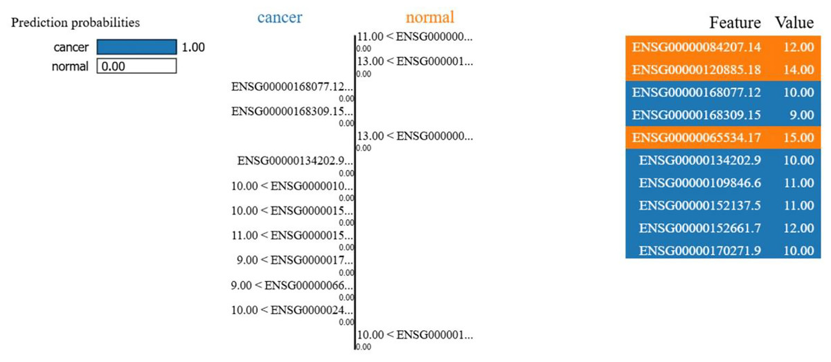
Figure 6: LIME interpretability result.
The LIME explanation of a representative prediction. Blue features contribute toward cancer classification, orange features toward normal. The model predicted cancer with probability 1.00, with the right panel showing the top contributing genes and their values.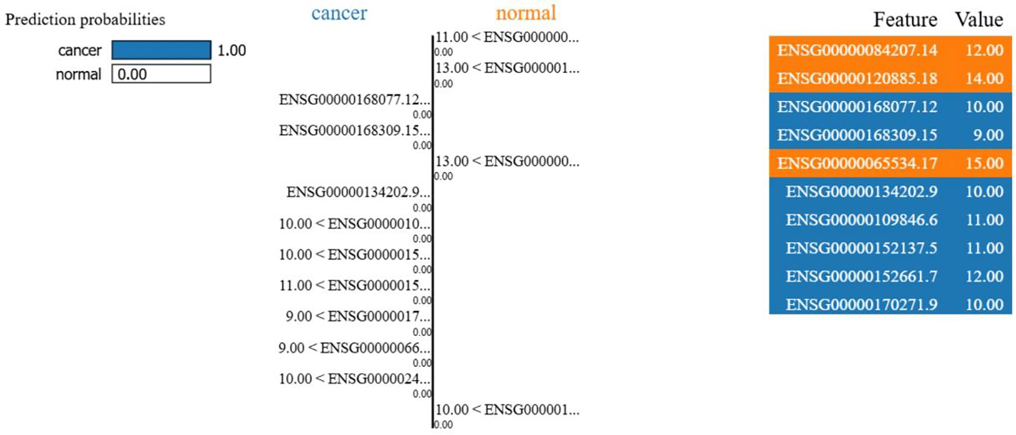
In Fig. 6, each gene’s expression reflects its activity value in the sample (e.g., ENSG00000084207.14 at 12.00 was more active than ENSG00000168309.15 at 9.00). Blue colored genes supported cancer predictions, while orange colored favored normal. This visualization supports model reliability, amid class imbalances. Interpretability focuses on the 13-gene dataset for clarity on key biological signals. Figure 7 ranks the top 13 gene by LIME importance, with higher bars indicating greater influence.
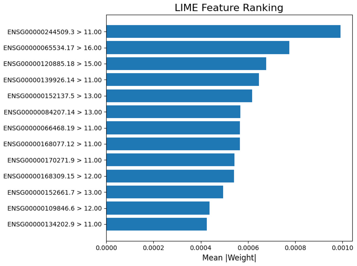
Figure 7: Lime feature ranking.
The LIME analysis of the model’s predictions, highlighting the top 13 gene features with the greatest average absolute contribution (mean |weight|). Each bar represents how strongly a gene influenced the model’s decision for classification, with higher weights indicating stronger predictive importance.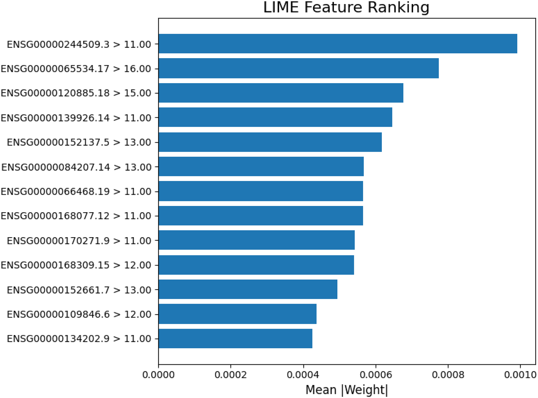
Model evaluation
This study optimized Gaussian naïve Bayes to achieve 95% accuracy. In comparison, a prior study using AdaBoost with feature selection techniques such as Sequential Floating Forward Selection (SFFS), RELIEFF, Sequential Backward Feature Section (SFBS) and Significant Attribute Evaluation (SAE) reported a 91.1% accuracy (Tirumala & Narayanan, 2019). This comparison highlights Gaussian naïve Bayes’ potential for gene expression datasets.
Discussion
The Gaussian naïve Bayes model demonstrates robust performance in detecting prostate cancer using limited gene expression data, achieving 95% accuracy in optimal scenario. The model excelled in recall, precision, and F1-score (up to 97%), effectively differentiating tumor from normal samples. Validation on Black race samples yielded 93% accuracy, highlighting unaddressed racial disparities in prior research.
Although the techniques employed are established in bioinformatics and machine learning, the novelty of this study lies in its comprehensive and race-specific framework. By combining DEG thresholds, ROC validation, balancing techniques, and hyperparameter tuning across 96 scenarios, effective feature combinations were identified White race prostate cancer detection. Additionally, LIME was used to interpret gene activity in cancer vs. normal predictions. This aspect has not been sufficiently explored in previous studies. Not all scenarios are detailed here due to inconsistent performance and to emphasize top outcomes; full results are available in the Supplemental File.
Feature selection impacted accuracy of Gaussian naïve Bayes model. In this study, all scenarios utilized DESeq2 to determine the most effective feature selection. Scenario 1 (basemean >= 10, padj < 0.05) averaged 94% accuracy but risked including irrelevant features without further thresholds. Scenario 2 (adding thresholds of basemean >= 10, padj < 0.05 and log2FoldChange < 0.35) filtered for highly expressed genes, yielding 92% accuracy. Scenario 3 (log2FoldChange <0.4) also achieved accuracy of 92%, suggesting limited benefit from this adjustment. Scenario 4 (basemean >= 10, padj < 0.05, ROC > 0.9) outperformed others, with ROC enhancing prioritization and performance.
Comparable studies include one achieving 94.11% accuracy with naïve Bayes on 179 features selected via multiple SFFS and SAE (Tirumala & Narayanan, 2016). Another study using chi-square test for naïve Bayes reported up to 67% accuracy (Antunes et al., 2025). This study surpassed these with 95% accuracy using fewer genes and race-specific focus.
For broader validation, a study employing Weka data mining tool for feature selection and SVM algorithms achieved 95.8% (Alkhateeb et al., 2019). These comparisons affirm the framework’s competitiveness, particularly with minimal features and race-specific validation.
Conclusion
This study implemented improved feature selection via DEG analysis and ROC analyses for prostate cancer detection using Gaussian naïve Bayes. Models with fewer genes achieved 95% accuracy, with recall, precision and F1-score reaching 97%. The minor accuracy difference between races indicates the need for race-specific approaches. Validation on Black race samples produced comparable performance of 93%, demonstrating model robustness while emphasizing the importance of race-aware diagnostics. The integration of LIME enhanced interpretability by identifying key genes influencing prediction outcomes. Limitations include small sample sizes, class imbalances, and fewer Black/normal samples, potentially affecting generalizability of the results. Overall, feature selection is crucial for developing race-based Gaussian naïve Bayes models.