
Lyapunov-based control for enhanced trajectory tracking in robotic arms using multi-objective particle swarm optimization
- Published
- Accepted
- Received
- Academic Editor
- Bilal Alatas
- Subject Areas
- Algorithms and Analysis of Algorithms, Autonomous Systems, Optimization Theory and Computation, Real-Time and Embedded Systems, Robotics
- Keywords
- Lyapunov-based control, Multi-objective particle swarm optimization, Robotic arm trajectory tracking, Pareto front
- Copyright
- © 2025 Lobato-Larios et al.
- Licence
- This is an open access article distributed under the terms of the Creative Commons Attribution License, which permits unrestricted use, distribution, reproduction and adaptation in any medium and for any purpose provided that it is properly attributed. For attribution, the original author(s), title, publication source (PeerJ Computer Science) and either DOI or URL of the article must be cited.
- Cite this article
- 2025. Lyapunov-based control for enhanced trajectory tracking in robotic arms using multi-objective particle swarm optimization. PeerJ Computer Science 11:e3397 https://doi.org/10.7717/peerj-cs.3397
Abstract
Robot manipulators have become a revolutionary tool in modern automation, medical interventions, service robots, rehabilitation systems, and service industries, acting as enabling methodologies to enhance the precision and reliability of many applications such as robotic-assisted telehealth. It is therefore evident that, to maximize functionality, large-scale and powerful control strategies need to be harnessed by such robotic systems. This work presents a new control scheme for two degrees of freedom robot arm based on Lyapunov PID control and Multi-Objective Particle Swarm Optimization (MOPSO). The proposed approach aims to consider reduction of tracking errors and control effort. These two objective optimizations simultaneously increase the precision of the trajectories and decrease the wear of the mechanism and energy consumption, which are invaluable properties for practical problems such as robot cutting and welding. The proposed approach demonstrates significantly better simulation performance with advanced reference trajectories, resulting in notable improvements in tracking accuracy and energy efficiency compared to well-established methods. By combining Lyapunov-based analysis with bioinspired multi-objective optimization, this work contributes to a more robust and reliable controller design framework for nonlinear robotic systems. The proposed framework thus provides a systematic solution for advanced robotic design by overcoming the limitations of heuristic or trial-and-error methods.
Introduction
Robotic manipulators are central tools for today’s automation, from surgical assistance to complex industrial assembly and operations in hazardous environments. Their applications involve areas where consistency and precision are essential. Strong and scalable control is essential in order to make full use of them. Among these, Lyapunov-based control is one robust pillar upon which nonlinear system control can rely for credible and predictable performances, even if conditions are variable or unknown (Hafsi, Gharsellaoui & Bouamama, 2022; Lv et al., 2023; Alattas et al., 2021; Yan et al., 2023). Recent progress in robot control emphasizes a growing demand for trajectory tracking strategies that remain reliable, even in the face of uncertainty, external disturbances, and physical constraints. A noteworthy example is the work by Tian et al. (2024), who developed a fully actuated system (FAS) for robotic manipulators. Their approach integrates high-order observers to estimate perturbation forces and applies gradient-based techniques to fine-tune control parameters. This control architecture is carefully designed to manage challenges such as unknown system dynamics, frictional effects, and constraint enforcement. Both simulation and experimental results demonstrated that the proposed method delivers robust tracking performance under complex and variable conditions. These results highlight the potential of combining model identification techniques with smart observer designs and finely tuned control gains to address the complexities of trajectory tracking in robotic arms. Alattas et al. (2022), explored the use of an adaptive sliding mode controller enhanced with barrier functions for unmanned aerial vehicles (UAVs), showing how it is possible to navigate the trade-offs between actuator limitations and uncertain dynamics while still maintaining stability and control. The Lyapunov-based stability analysis and the results of the computer simulation presented and met with reliable finite time tracking performance under the impact of perturbing actions, and they revealed the competence of advanced nonlinear methods within the robotics control field. Considerable emphasis has been placed on resolving the problem of enabling trajectory tracking with increased precision in robot manipulators under the impact of uncertainty.
Wang et al. (2024a) suggest the prescribed performance adaptive robust control (PPARC) scheme, which combines the fuzzy set theory for uncertainty representation and relies on Lyapunov for stability analysis. Most importantly, the method is suitable for ensuring the accuracy of tracking within a prespecified region, even under the impact of time varying intricacies and unknown initial states. Furthermore, the article suggests the formulation of the optimal settings of controller parameters within an optimization fuzzy-based form, and it delivers both theoretical stability proof and experimental evidence through the computer simulation of a two-link robot manipulator. In the past two decades, the advancement of adaptive and robust control techniques has continued with further momentum, even for biomedical applications, particularly for highly complex nonlinear dynamics. In an example application, Mokhtare et al. (2022) developed an adaptive barrier function terminal sliding mode control methodology specifically designed for waveform suppression in epilepsy using the nonlinear Pinsky Rinzel epilepsy dynamics. In this methodology, the terminal sliding mode for finite-time stable dynamics is combined with an adaptive barrier function for robustness against uncertainty and external disturbances to ensure stability. In robotics for rehabilitation, Sun et al. (2024) suggest a novel event-triggered critic learning impedance control approach for interactive control of lower limb exoskeletons. The system formulates the impedance control issue within the framework of optimal control and employs reinforcement learning for adaptation of user and environment dynamics. Compared to periodic schemes, the controller developed triggers learning events when the state undergoes significant changes to improve performance. Aly et al. (2022) developed a fuzzy-based fixed time nonsingular terminal sliding mode controller, aided by a state observer, for upper limb exoskeleton robots for rehabilitation. Fuzzy logic is utilized to minimize chattering and ensure fixed-time error in tracking to reveal strong performance and precision for different initial conditions. The results suggest the potential for the combination of observer design, fuzzy control, and sliding mode for performance optimization of assistive robotics.
It has been shown that advanced optimization and control techniques are applicable to a broad variety of practical problems. Take, as a case study, surgery robotics, where accurate and robust trajectory tracking becomes important, firstly, to achieve a higher surgery procedure success rate, and secondly, to patient safety (Xie et al., 2024; Sachan & Swarnkar, 2023).
In automation and robotic services, energy efficient control strategies are significant to promoting sustainability and minimizing operational costs and are consequently very well suited to large-scale industrial applications. For a new area such as micro robotics, with stringent size, power, and precision constraints that prevail during system design, sophisticated techniques of control are inevitable. All these diverse applications serve to underscore the depth and increasing relevance of sophisticated techniques of control as a tool to overcome the complexities of modern robotic systems. In industrial robots and robotic manipulators, adaptability to changing flexible manufacturing environments, complex assembly tasks, and cooperative work with human coworkers require direct mappings of stability and optimized control effort to productivity and worker safety levels (Arents & Greitans, 2022). In service robots such as in logistics robots, agricultural robots, and autonomous warehouse robot’s efficiency in energy consumption, adaptability to changing environments and configurations, and suppression of external disturbances translate to cost effectiveness and sustainability in operations (Choi et al., 2024; Yepes-Ponce et al., 2023; Yang et al., 2025). Finally, improvements in rehabilitation robotics and exoskeletons require controllers to achieve smooth, precise, and consistent assistance under variables and changing circumstances (Mashud, Hasan & Alam, 2025). Whereas related works on industrial, service, and rehabilitation robotics have indeed provided important contributions like increasing adaptability to changing environments, improving energy efficiency, and realizing accurate assistance in rehabilitative and medical applications, many are concerned with single objective optimization or traditional tuning of the controller gains. These tend to neglect the trade-off among tracking quality and control effort and hence are restricted in adaptability across multiple-criterion tasks of greater complexity.
In this work, we examine how the Multi-Objective Particle Swarm Optimization (MOPSO) enhances the performance of the Lyapunov-proportional–integral–derivative (PID) controller when compared to both the standard Lyapunov-PID and traditional PID controllers in the context of a two degrees of freedom (DOF) robotic system subjected to disturbances. The experiments evaluate performance on complex trajectory profiles, including gear spiral and rose curves. Our extensive analysis shows that the Lyapunov-PID controller optimized by MOPSO, significantly reduces steady state error, minimizes mean squared error (MSE), simultaneously optimizes accuracy and energy efficiency, decreases overshoot, and enables a faster recovery following disturbances. This article presents MOPSO and coupled-PID control with Lyapunov for the first time, such that tracking precision and control effort, both, could be optimally tuned simultaneously.
The rest of the article is outlined as follows. ‘Theoretical Foundations’ states the theoretical basis, outlines the mathematical modeling of the 2-DOF robot arm, its kinematics, dynamics, and the Lyapunov-based control system. ‘Proposed Methodology’ describes the methodology, formulates the algorithm for MOPSO, its structure, its parameterization, and its integration with the control system. ‘Results and Discussion’ presents the results, comparing simulation performance between the optimized and calibrated controller with MOPSO, with an eye toward important performance factors such as tracking accuracy, control effort, and overshooting. Finally, some concluding remarks for this work are presented in ‘Conclusions’.
Theoretical foundations
Particle Swarm Optimization (PSO) was introduced by Kennedy and Eberhart in the mid-1990s, inspired by the social behavior of flocks of birds (Zeedan, Attiya & El-Fishawy, 2022; Li, Yan & Qu, 2020; Yang et al., 2023). Over the years, research has enriched the method with adaptive strategies, multi-objective variants, and hybrid approaches to improve convergence and the ability to escape local minima (Wang et al., 2024c; Ram et al., 2020).
Fundamental equations
In the classical PSO algorithm, each particle i has a position vector and a velocity . At iteration , these are updated as follows (Zeedan, Attiya & El-Fishawy, 2022; Li, Yan & Qu, 2020; Yang et al., 2023).
(1) where is the inertial weight, is the cognitive coefficient, is the social coefficient, and are random scalars in [0, 1], is the best position found by the particle , and is the global best among the swarm (or a neighborhood best in local PSO variants).
Position update step
Proper selection of , , and strongly affects global exploration vs local exploration (Lobato-Larios, Starostenko & Alarcon-Aquino, 2024; Li, Yan & Qu, 2020; Yang et al., 2023).
PSO for multi-objective problems
In many real-world control applications, it is common to have multiple objectives that often conflict with each other. For instance, in robotics, minimizing tracking error may conflict with minimizing energy consumption: pushing the system to follow a path with very high precision typically requires additional torque, thus consuming more energy. When there are many aims to be optimized simultaneously, the Pareto front idea (or a set of non-dominating solutions) is gaining significance (Wang & Zhou, 2024; Sun, Deng & Li, 2020; Li, Zhang & Hu, 2023; Ma et al., 2025).
Non dominated solutions
A solution is said to dominate another solution if and only if:
-
1.
is not worse than in all objectives, and
-
2.
is strictly better in at least one objective.
In contrast, a solution is non-dominated if no other solution in the population (or archive) dominates it. The collection of all such non-dominated points constitutes the Pareto front. Each point on the front represents a distinct trade-off between objectives. Key enhancements in MOPSO include diversity preservation (via crowding distance) to maintain a uniform approximation of the Pareto front. Adaptive coefficients (w, ) to favor exploration at early stages and exploitation at later ones (Barba-González et al., 2020; Xu, Zhang & Chen, 2020). Mutation or perturbation operators to avoid stagnation in suboptimal regions (Wang et al., 2024c). Rather than finding a single “best” set of improvements, it is possible to choose between a range of equivalent bests. That is, a marginally increased tracking error can be tolerated when it reduces power consumption (or vice versa). By viewing the entire Pareto front, it is possible to determine which performance criteria hold more weight (precision vs energy, accuracy vs cost, etc.).
MOPSO algorithm
MOPSO is an extension of the original PSO algorithm developed to deal with several objectives and produce a Pareto front instead of a single global optimum. Classical PSO aims for a single optimal (global best) solution, but MOPSO retains and updates an external archive (or repository) of non-dominated solutions. The archive then leads to the swarm during movement in the search space. At each iteration, the particles are evaluated considering various objectives (e.g., tracking error and energy consumption). The algorithm adds all newly found non-dominated particles to the archive and eliminates existing solutions found to be dominated by the newcomers. The MOPSO tends to choose one or several of the “leaders” from the archive to influence the velocity update of the particles. Instead of a single leader, there might be multiple leaders, each of which is equally valid for Pareto dominance. Each particle still maintains its personal best ( ), but when searching for the global best, MOPSO randomly chooses one solution (a “leader”) from the external archive. This leader selection can use strategies, such as roulette wheel based on crowding distance, or simply random selection among all non-dominated solutions. Over iterations, individual experience ( ) and diversity of leaders (the non-dominated solutions in the archive) are utilized by the swarm.
Ideally, particles will settle down to a well-diversified Pareto front, offering several trade-off solutions. Throughout the optimization process, MOPSO may adapt the inertial weight w and the cognitive/social factors , . A high inertial weight induces overall search in early iterations, and a low inertia weight aids in refinement locally (exploitation) in later iterations. This mechanism can become a critical feature in evading early convergence to a local Pareto front and in having an ideal balance between searching new regions and enhancing the current best collection of solutions (Barba-González et al., 2020; Xu, Zhang & Chen, 2020; Ma et al., 2025; Wang & Zhou, 2024; Yang et al., 2023), MOPSO naturally handles distinct objectives in parallel. Maintaining an external archive gives a global vision of search progress, pointing out which solutions are currently non dominated and ensuring that valuable trade-offs are preserved. Once the algorithm terminates, the final Pareto front can be inspected and the solution that best fits the practical constraints can be selected (e.g., a midpoint solution balancing moderate energy usage with acceptable accuracy).
Kinematics and dynamics of a 2-DOF robotic manipulator
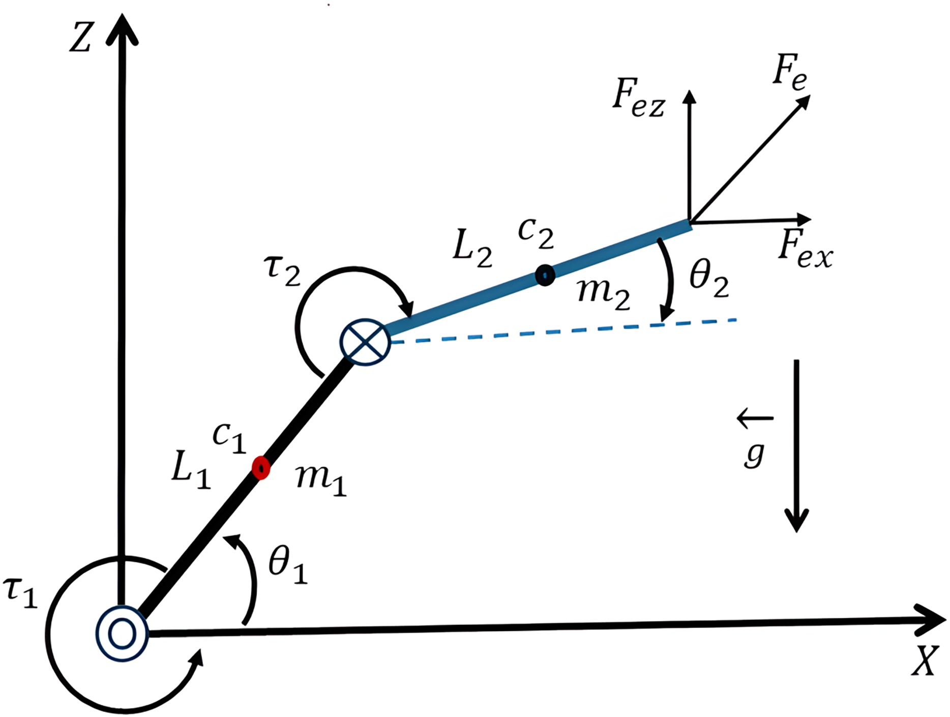
Robot manipulation is commonly in the form of nonlinear, coupled dynamics, presenting difficulties for typical control schemes (Alattas et al., 2021; Yan et al., 2023; Craig, 2022). A 2-DOF planar manipulator is composed of two rigid links that are connected through revolute joints, as depicted in Fig. 1. The following variables should be defined:
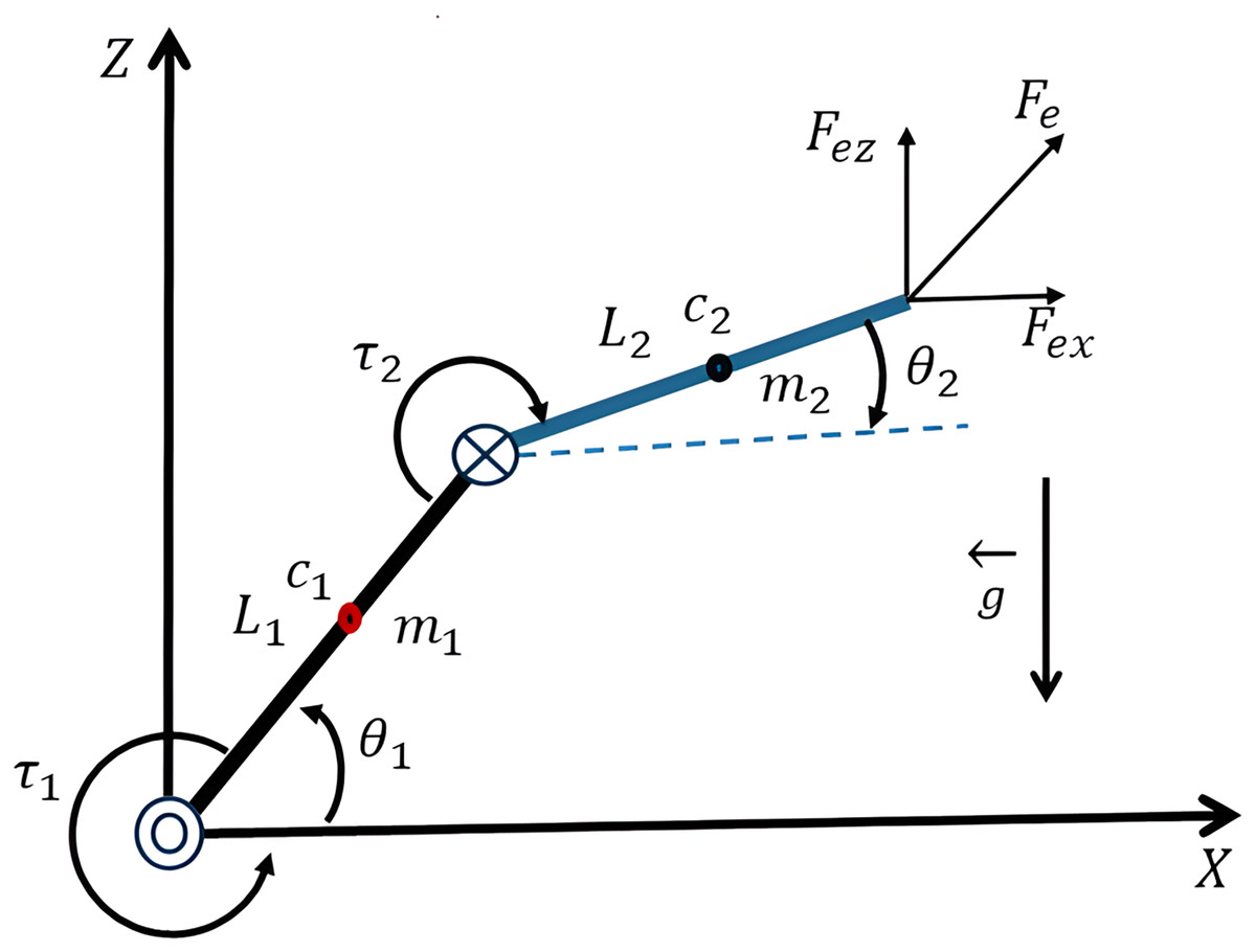
Figure 1: Kinematic representation of a two-segment system.
The angles of the joints, and , in terms of angles relative to a reference axis; the length of the links as the quantities and ; the mass of the first and second links as the quantities and , respectively; the vector is the gravity, acting upon the masses in the negative Z; the location of the centers of mass for the first and second links as the quantities and , respectively; the control torques acting on the first and second joints, so that and respectively, are the quantities that drive the motion of the first and second links, so that the motion of the end of the second link follows the desired motion in the plane, and is the external force acting upon the end-effector, decomposed along the and .
Kinematic and dynamic modeling of the 2-DOF robot manipulator
Assumptions
Rigid links: Connections are idealized as completely rigid; elastic or compliant deformations are also disregarded. This simplification of the dynamics, however, does not significantly affect accuracy at the involved size and material scales (Liu et al., 2023).
Ideal revolute joints: All the revolute joints are assumed to be ideal for the scope of this study. There is no backlash or mechanical play. Precision actuation mechanisms and joints are so advanced these days that all such faults are nullified. We assume the consequential effects to be negligible for the purpose of estimating the performance evaluation of the controls (Gamez-Herrera et al., 2025).
Joint friction model: Joint friction is a mixture of viscous (linear), and a constant (Coulomb), element friction. This accounts for the normal friction behavior balancing simplicity and effectiveness without introducing unnecessary complications associated with nonlinear modeling (Shao et al., 2023).
Known time-invariant parameters: Physical quantities such as lengths, masses, inertias, and gravity acceleration, are considered as being precisely known and constant during simulation.
Planar motion constraint (ZX plane): The 2-DOF robotic arm can translate along the ZX plane with a steady position at the Y axis. With this constraint, dynamic and kinematic modeling become simpler (Soleymani & Kiani, 2024).
External disturbances: Although external upsets are used within narrow time slots within a simulation to mimic events like sudden payload changes or external shock, a systemic study regarding a controller’s robustness and disturbance rejection capability to disturbances can be assisted.
The system operates within joint limits: . Workspace constraints are imposed to avoid unreachable trajectories .
Kinematic model
Given joint angles :
(2)
(3)
(4)
(5) where is the end-effector position.
The Euler Lagrange formulation leads to the Eq. (6) of motion (Alndiwee, Al-Mahairi & Hamdan, 2022).
Dynamic model
The equations of motion for the manipulator are given by:
(6) is the inertia matrix, is the Coriolis matrix, is the gravity vector, is the friction vector, is the joint torque vector, is the vector of external disturbances.
Inertia Matrix:
(7) with:
(8)
(9)
(10)
(11) are the moments of inertia of links 1 and 2 with respect to their centers of mass, respectively; are the masses of link 1 and link 2, respectively; are the lengths of link 1 and link 2, respectively; is the cosine of the second joint angle.
Coriolis and Centrifugal Matrix
(12) where
(13)
(14)
(15)
(16)
(17) are the angular velocities of joint 1 and joint 2 respectively; is a parameter that captures the coupling effects between the two links resulting from Coriolis and Centrifugal forces.
Gravity Vector
(18)
(19)
(20) is the acceleration due to gravity. represents the gravitational effect on both joints, considering the mass distributed along the first link (up to its midpoint) and the total mass of the second link, as well as the contribution of the second link in both joint directions, accounts for the gravity contribution acting only the second link, projected along the second joint axis.
Friction Vector
(21) where are viscous friction coefficients, and are Coulomb coefficients.
Physical constraints
Joint limits are restricted to physical actuator ranges, all generated trajectories are tested to ensure they are within the reachable workspace , applied torques are saturated to actuator limits.
Lyapunov PID based control and integration with MOPSO, stability in nonlinear systems.
Lyapunov based control ensures stability by defining a Lyapunov that is positive definite. The control law is then designed so that , guaranteeing error convergence (Yang et al., 2023; Wu et al., 2019). For a 2-DOF manipulator, let position error and velocity error. Lyapunov is utilized for establishing the stability of PID controllers in nonlinear systems, or in disturbances, tuning parameters, and so the system energy is constantly decreasing, the proportional term adjusts error size, and the derivative term avoids overshoot and suppresses vibrations, and the integral term eliminates steady-state error, ensuring that the accumulated tracking error is minimized (Xu, Zhang & Chen, 2020). PID is utilized in conjunction with Lyapunov based analysis to enhance stability (Zhang, 2023; Orlov, 2020). The PID control law can be written as
(22)
(23) where , , and are the proportional, derivative and integral gain matrices.
In our proposed approach, gains of the trajectory tracking controller ( , ) are not predefined with fixed numbers. These gains are automatically optimized within predefined ranges using the MOPSO optimizer. These ranges are predetermined from a priori knowledge of the system based on the best values of MSE, SSE, and OVSH and are deemed probable areas of stable and efficient control. System optimization occurs through simulation of the robotic system with bounded disturbances as a measure of robustness and performance.
For the standard PID controller as a base reference point, the gain settings ( , ) were established through a similar process as used with the Lyapunov-PID controller MOPSO optimization. However, instead of utilizing a population-based search within predetermined bounded intervals, an empirical performance analysis and iterative refinement were undertaken through a manual tuning process. When a satisfactory set of fixed gains were established, constant gains were utilized during all of the subsequent simulations. Importantly, an identical gain set was also used with the Lyapunov-PID formulation (with no subsequent optimization) so that a consistent and fair comparison could be established between both control methods (Lyapunov-PID, and PID only).
Once the initial space of parameters is established by practical constraints and initial results, neither the gains of the control ( , , ) are static nor constant. Instead, they are varied in each program run by the implementation of the MOPSO algorithm. In the initialization of each run, the program establishes a population of particles where each particle is another potential solution carrying various sets of , , and randomly initialized within the established minimum and maximum restrictions. Performance of each potential solution is scored using two opposing objective functions (e.g., tracking error and control effort), which are established through simulation. During the process of repeated optimization, the parameters of each particle are modified relative to the best performance of the past and the best solutions encountered in the population (the Pareto front). The algorithm is kept searching for the parameter space in an interplay between stochastic exploration (to avoid the local minima trap) and social learning of the best performers. It repeats the process until the optimum number of iterations is attained. The outcome is the set of Pareto-optimal solutions, for which the best gains are selected for performance evaluation and simulation. It is guaranteed by the method presented here that the controller is methodically tuned for each trajectory and for each level of disturbance.
Gain optimization with MOPSO
To overcome heuristic or trial-and-error tuning, MOPSO can be employed as follows (Wang et al., 2024c):
-
1.
Define objectives:
: tracking error.
: control error.
-
2.
Set feasible ranges for the gains .
-
3.
Optimization loop:
Each particle represents a candidate .
The robot’s dynamic simulation computes for that candidate.
Non-dominated solutions are stored in Pareto repository, guiding the swarm’s evolution.
By combining Lyapunov stability with MOPSO’s capability to search multi-objective spaces, one obtains robust and efficient gain values (Barba-González et al., 2020).
Trajectory generation
We consider various end effector paths. Besides simple shapes, we include more intricate patterns to challenge the controller across wide operating ranges. Given (xd(t), zd(t)), we obtain through forward differentiation and inverse kinematics (Hernandez-Barragan et al., 2022).
Multi-objective fitness formulation
Tracking Error :
(24) quantifying joint space deviation (Dorf & Bishop, 2022).
Control Effort :
(25) where T represents the total time interval for which the integral is calculated representing torque or energy usage (Dorf & Bishop, 2022).
represents the mean squared joint-space deviation and directly quantifies tracking accuracy; measures the time-averaged absolute torque, capturing the total mechanical impulse delivered by the actuators.
Hence, the MOPSO-based optimization problem is:
Let
denote the vectors of proportional, derivate, and integral gains.
The multi-objective optimization problem is stated as
(26) The feasible set a MOPSO algorithm is employed to construct a Pareto front of non-dominated solutions, providing a spectrum of gain combinations that balance tracking accuracy against actuator effort.
Proposed methodology
The study takes a 2-DOF robotic arm, whose function is to follow a desired path in the ZX plane with high accuracy. Two joints make up a robotic arm with dimensions and , respectively. Two motors actuate each of the joints, with an ability to apply torques in a range of ±100 Nm. Inertia, Coriolis, forces, gravitational, and frictional (viscous and Coulomb friction) terms make up dynamics of robotic arms. For actuating joints angles of robotic arm, a PID controller with a basis in Lyapunov stability was adopted. Controller creates torques ( ) to drive down total error ( ) between desired and actual path of robotic arm. The control law is described by Eqs. (27) and (28):
(27)
(28) where:
is the position error and represents the difference between the desired joint angle and the actual joint angle at any given time.
measures the speed of the tracking error over time.
is the integral of the position error.
and are the joint angles and angular velocities.
and are the desired joint angles and angular velocities.
M, C and G represent the inertia matrix, Coriolis matrix, and gravitational forces respectively.
accounts for viscous and Coulomb friction.
, , and are the proportional, derivative and integral gain matrices, respectively.
To enhance the performance of the PID controller, the gains , , and were optimized using the MOPSO algorithm. Table 1 shows the key parameters and configurations (Barba-González et al., 2020; Xu, Zhang & Chen, 2020; Wang et al., 2024b).
| Parameter | Description | Value used |
|---|---|---|
| Number of particles | The size of the swarm, representing the population of solutions explored simultaneously. | 175 |
| Number of iterations | The total number of optimizations cycles the algorithm performs to cover optimal solutions. | 10 |
| Inertia weight (w) | Controls the impact of a particle’s previous velocity, balancing exploration and exploitation. | 0.65 |
| Cognitive coefficient ( ) | Represents the influence of a particle’s individual best position on its velocity update. | 1.98 |
| Social coefficient ( ) | Represents the influence of the swarm’s global best position on a particle’s velocity update. | 2 |
Optimization objectives
Minimize Total Error ( ): quantified using the mean squared error (MSE) between the desired and actual trajectories.
Minimize Control Effort ( ): Measured by the integrated absolute torque applied over the simulation period.
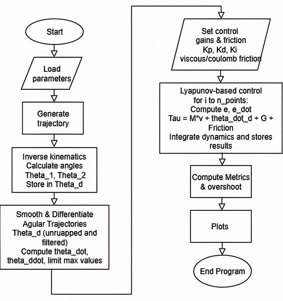
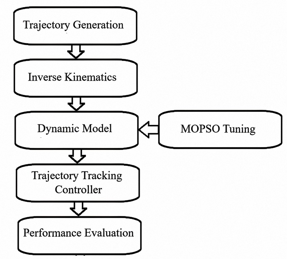
A PID based on a Lyapunov function is employed in this work (see Fig. S1 in Supplemental Files). The input parameters are set first. The system designs a desired path (gear-shape and rose curve), followed by a robotic arm. Inverse kinematics is utilized by the system to identify the needed angles and positions to track a desired path. For the flowing and smooth motion of the system, resulting paths in angles are differentiated and smoothed, computing the accelerations along with the velocities of the angles. The system is then controlled using a Lyapunov PID based, which is created on the error signals, their derivatives, and their integrals that have been computed and utilized in the dynamic adjustment of the control. The system is then tracked using the computation of parameters such as overshoot. Finally, the system plots the computed results.
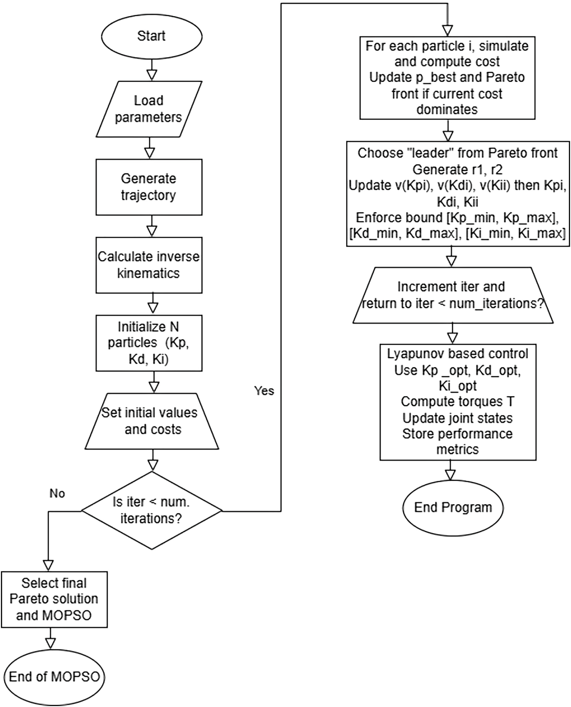
One of the proposed strategies in the process of research is the optimization of parameters and Lyapunov based PID control using MOPSO (see Fig. 2). The process begins with the loading of parameters and trajectory. Inverse kinematic computations are conducted in the determination of joint angles to go along a given path. The process begins with the initialization of an initial set of candidate solutions using random generation based on given limits. Each of these is given an initial cost using the given performance metrics. The iterative MOPSO optimization is conducted to determine the best controlling gains. In each of these iterations, it checks for the satisfaction of the stop criterion, i.e., the number of iterations. If not, all these particles are simulated, and each of these is cost-computed, compared against past best, as well as compared against the Pareto front, and these are updated when the current solution dominates the past solution. One of these is chosen as a leader based on random coefficients of ( , , Eq. (1)), and each of these velocities is updated for , , and .
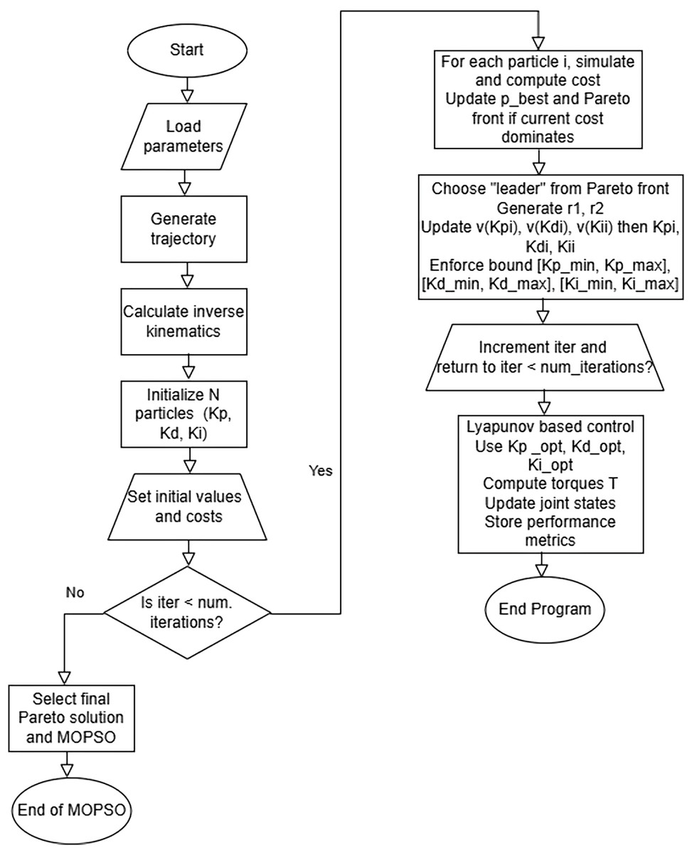
Figure 2: Control Lyapunov-based PID control optimized with MOPSO.
The new parameters are constrained using given limits of , and for controlling parameters. The counter is incremented. At the termination of optimization, a Pareto optimal point is selected. The optimized gains are input in each structure of a Lyapunov PID based. Performance metrics are recorded for evaluating the optimization of the controller. Finally, it terminates, which concludes MOPSO optimization.
Simulation setup
All the simulations for the present work were executed on MATLAB R2023a (The MathWorks, Inc., Natick, MA, USA). The simulation environment was designed using MATLAB script files, exploiting maximum use of its computational and visualization facilities. The simulations were executed in a Windows 11 environment installed on an Intel Core i9 CPU and 32 GB RAM. The simulation protocol followed an ordered sequence of the following steps.
Trajectory generation: A gear-like and rose curve reference trajectories of the end effector of the robot in the ZX plane were designed such that all the target points are within the reachable workspace of the manipulator.
Inverse kinematics: The joint angles for every point in the trajectory are computed using a special analytical inverse kinematic function, specially designed for the two-link planar manipulator.
Modeling and implementation of dynamic control: The nonlinear dynamic model of the two-link robot was designed, considering physical parameters, the effect of friction, and external agencies. A Lyapunov-based PID controller has been employed in the simulation loop to track of the trajectories.
Tuning of the controller using MOPSO: Multi-objective particle swarm optimization algorithm is used to fine-tune of the PID gains ( , ) in the Lyapunov–PID controller. The optimization is for the simultaneous minimization of the tracking error and the control effort by the composite cost function.
Simulation and performance measure: The closed loop system is simulated for the total trajectory. The performance parameters, such as mean squared error (MSE), overshoot, steady state error, and actuator torque, are employed to quantify the performance. Also, they are plotted for pictorial representation. A schematic of simulation architecture is presented in Fig. S2 in the Supplemental Files section. It shows the key modules and the flow of information.
The simulation parameters are shown in Table 2 (Craig, 2022; Spong, Hutchinson & Vidyasagar, 2020; Sciavicco & Siciliano, 2000).
| Parameter | Description | Value used |
|---|---|---|
| Total simulation time | The duration over which each trajectory is executed. | 260 s |
| Time step | The discrete interval between simulation steps. | 0.009 s |
| Number of simulation points | Calculated based on total and time step | 28,888 points |
| Link lengths | Lengths of the robotic arm’s links | |
| Masses | Mases of the robotic arm’s links | |
| Moments of inertia | Inertia of the robotic arm’s links | |
| Gravity ) | Acceleration due to gravity | |
| Friction coefficients | Parameters modeling viscous and Coulomb friction |
Three distinct paths have been taken to evaluate the performance of the controller (the spiral and rose curves are included in the Supplemental Files). Gear path, with sharp intersection and rotational trends. Let be the number of gear teeth, the tooth fraction, the number of points for the base arc, the root (base) radius, the tip radius, and the center coordinates of the gear.
Let index the gear teeth. For each , the following parameters are defined:
(29) The gear shaped trajectory is constructed by sequentially connecting the following segments for each tooth. Radial ascent: From base radius to tip radius at angle . Tip arc: an arc of radius spanning the angular range . Radial descent: From tip radius back to the base radius at angle . Base arch. An arc of radius spanning the angular range discretized into points for smoothness. Each segment is converted to Cartesian coordinates via (Stewart, Clegg & Watson, 2021).
(30)
(31) where denote the trajectory center, and and are the segment specific radius and angle.
Performance metrics
Appropriate procedures were implemented to maintain fairness, such as testing all the controllers using the same system dynamics, initial conditions, and perturbation scenarios. To maintain an open assessment of all the control strategies implemented within the present research work, the next methodology is followed. First, the mathematical representations and implementation aspects of all the controllers have been provided in fine details, along with the structure of the controllers, the parameter settings, and algorithmic routines of the controllers. The same conditions of the system dynamics, initial states, and sequences of perturbations, illustrated in the experimental setup, have been used for comparing all the controllers. The same set of performance metrics are employed for comparison to facilitate direct and objective evaluation. They comprise classical control metrics e.g., overshoot, steady state error, and mean squared error as well as some additional metrics of special interest in robotics, such as the total control effort, maximum per joint torque, and recovery time after perturbation. Each of the metrics is defined rigorously in mathematics as follows (Song, Li & Zhang, 2024; Siciliano, Sciavicco & Oriolo, 2021; Rivera et al., 2020; Elsisi et al., 2021).
Overshoot (OS) measures the maximum amount by which the system output exceeds the desired value following a reference change, expressed as a percentage of the total reference change. It indicates the tendency of the system to “overreact” before setting.
(32) where is the output value after the step change or reference shift, is the value attained by the system output after the reference shift, is the initial reference value (prior to the reference change).
Steady-State Error is the net error between the output and the reference after the system is in steady state, i.e., after all the transient effects have faded. It indicates the ultimate precision of the system.
(33) where is the error in time , is the steady-state interval, is the final time of the simulation/experiment.
MSE quantifies the average of the squared tracking error over the entire operation or simulation. This metric globally assesses tracking accuracy, with larger errors weighted more heavily.
(34) where is the number of samples, is the required value or path of the sample, is the true system output or the sampled value of the system output of the sample, is the value of the sample time.
Total Control Effort is the total of the actuators’ effort over time and is the integral (or sum) of the absolute value of the control inputs. It is the “energy cost” of control.
(35) where is the number of joints, is the number of time steps, is the controller output (torque command to joint at time , is the size of the time step.
Maximum Torque per Joint encompasses the experiment or simulation specified maximum value of torque being put on the robot’s individual joints. It is used to measure actuator requirements and to ensure the operational constraints are never violated.
, where is the control torque at time corresponding to the joint .
Recovery Time after Disturbance is the time needed for the system to reach again a small acceptable error (say, two times the static error) after the occurrence of an external disturbance, considered independently for the Z and X axes. It is an indication of the robustness and the disturbance rejection of the system. For the given disturbance applied between to .
For axis X:
(36) for axis Z:
(37) where , are the recovery time after perturbation for the axes Z and X, respectively; and are the initial and the end time, respectively of the applied perturbation; , are the absolute value of the tracking error for the axes Z and X, respectively at moment ; and are the steady-state error for the axes Z and X, respectively.
To verify the performance for the optimization of the MOPSO, the nonoptimized Lyapunov-based PID and the PID controller are also contrasted. The PID controller and the Lyapunov PID applied the initial tuning with preliminary experiments resulting in constant , , and gains. Comparing the simulation results reveals significant improvements in controller performance from MOPSO, underscoring the value of using MOPSO to design effective robot control strategies. The necessity of a systematic and scientific method of selecting the gains of the PID and of stability analysis according to Lyapunov based on the theory of robot manipulators has also been emphasized in literature. For example, Hernández-Guzmán & Orrante-Sakanassi (2019) presented a globally asymptotically stable scheme of PID for multi-joint manipulators using Lyapunov theory for which they demonstrated stability and, through simulations, verified the performance of the control with properly selected gains of the PID. Their findings characterize support for the necessity of stability-guaranteed PID, as well as for introducing methodical selection techniques of gains, like in the current work, using MOPSO.
In addition, Amiri & Ramli (2022) developed a Lyapunov-based adaptive PID controller for multi jointed robotic arms, comparing several gain initialization strategies and showing that correct gain selection enhances simultaneously tracking performance and robustness of the system. Similarly, Qiao et al. (2021) developed two adaptive PID controllers for robotic manipulators that ensure local asymptotic convergence of joint position and velocity tracking errors without requiring any equality or inequality constraints on the control gains. Unlike classical and other adaptive PID approaches, their proposed controllers offer enhanced robustness against dynamic uncertainties, even when the upper bound of such disturbances is unknown. Both controllers were analyzed using Lyapunov stability theory, which formally proved closed-loop stability and boundedness of the parameter estimation errors. Simulations on a two-degree-of-freedom planar manipulator demonstrated superior performance in tracking accuracy and disturbance rejection compared to classical PID, adaptive PD, LADRC, and NDOB-PID controllers. Their findings also highlight the potential importance in including advanced optimization and stability analysis, as discussed in the current contribution, for obtaining robust and high-performance controllers for robotic manipulators. By combining Lyapunov-based analysis with multi-objective optimization, the current contribution moves towards a systematic and dependable controller design procedure for nonlinear robotic systems, surpassing the limitations of heuristic or solely trial and error adjustment procedures.
Results and discussion
In this study, the MOPSO algorithm was used for optimizing a two-link robotic arm’s proportional ( ), integral ( ), and derivative ( ) gains of a Lyapunov based PID controller. The designed controller was capable of following elaborated motion profiles, i.e., gear-shaped, spiral and rose curve types, and its performance was optimized for minimizing both the total error ( ) and control effort ( ), in an attempt to have an optimal level of precision and effectiveness in terms of energy consumption. For evaluation purposes, an analysis with a non-optimal Lyapunov-based PID controller and PID control was incorporated to evaluate the performance of the proposed approach based on MOPSO. The optimization for each of these types of trajectories, i.e., gear-shaped, spiral, and rose curve, is conducted individually, and for each, a Pareto front for a specific tracking accuracy and control effort scenario is generated.
The results for the spiral and rose-curve trajectories are included in the Supplemental Files.
Gear shape trajectory
The comparative results demonstrate performance improvement when utilizing the MOPSO-Lyapunov-PID controller over results utilizing Lyapunov-PID and conventional PID control schemes. Specifically, steady-state errors of the X and Z axes are minimized by at least 43–50%, resulting in improved accuracy for trajectory tracing. MOPSO-Lyapunov-PID achieves notable accuracy gains, the MSE decreases by up to 93% in X and 77% in Z, indicating closer alignment with the desired trajectory. Transient behavior is also improved, overshoot is reduced by more than 80% in X and by 57–64% in Z relative to non-optimized controllers, yielding a smoother and more stable response. These improvements are achieved at a modest cost, the total control effort increases by only ~1.6%, a minor trade-off given the pronounced improvements in tracking accuracy and robustness. The recovery rates following the occurrence of a disturbance are significantly enhanced by the MOPSO-Lyapunov-PID, after the introduction of a disturbance in X, they are roughly 85–90% faster, and in Z roughly 90% faster than for the other schemes.
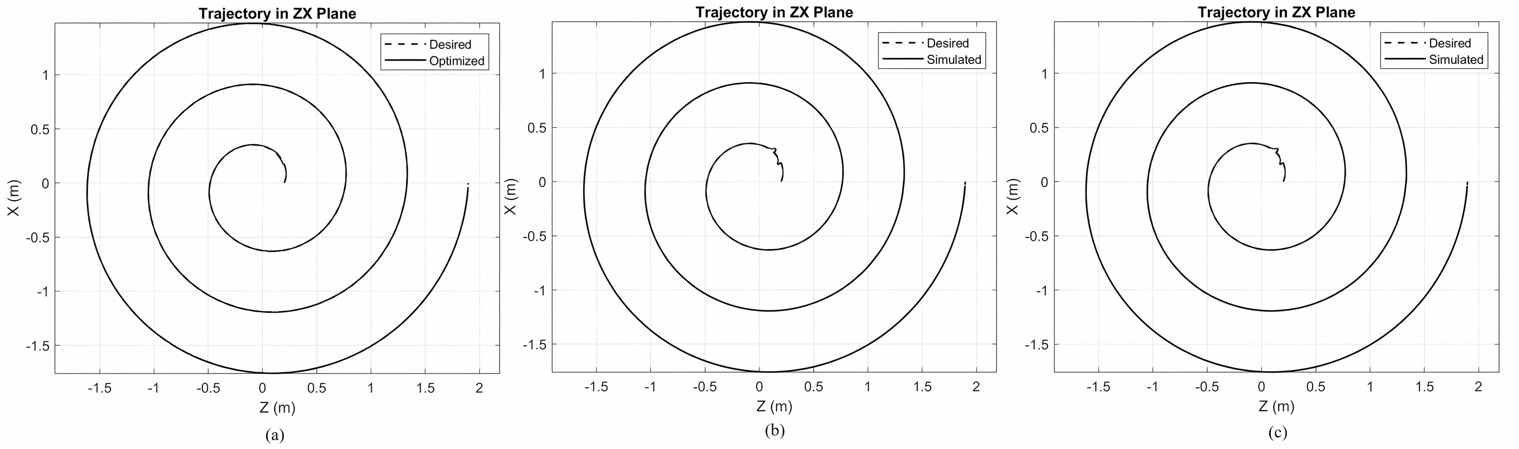
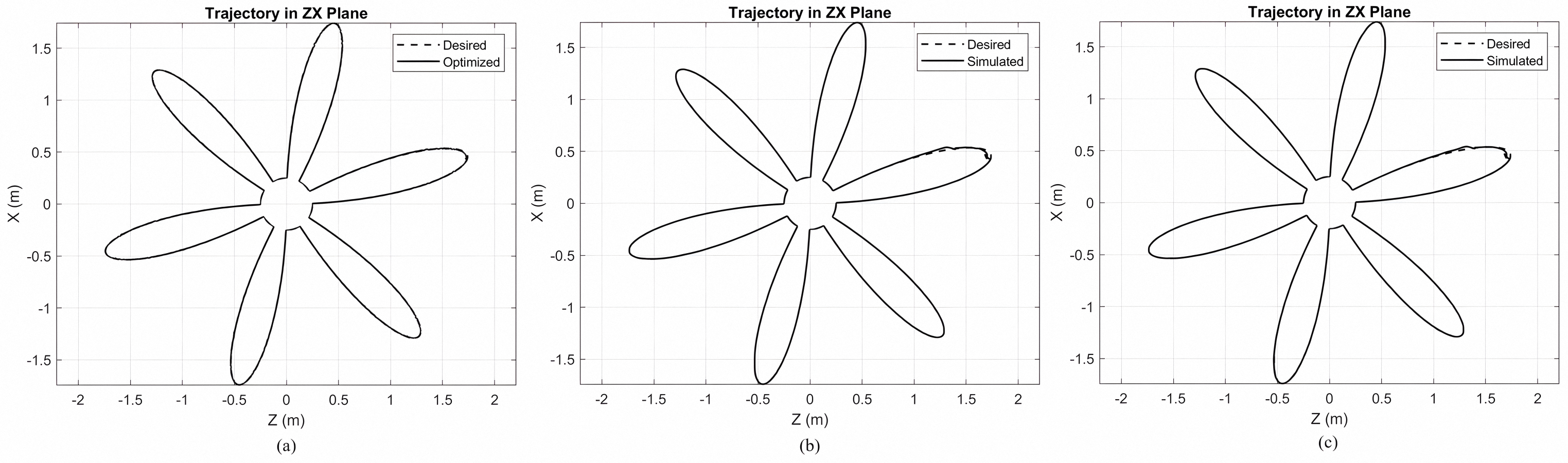
The simulation plots of the track of gear shape are given in Fig. 3. This figure shows the desired trajectory and the subsequent trajectory for three controllers: (a) the optimized Lyapunov-PID, (b) the non-optimized Lyapunov-PID, and (c) the PID-only controller. The desired trajectory is represented by dashed lines, and the subsequent trajectories of the non-optimized and optimized controllers can be observed from this figure.
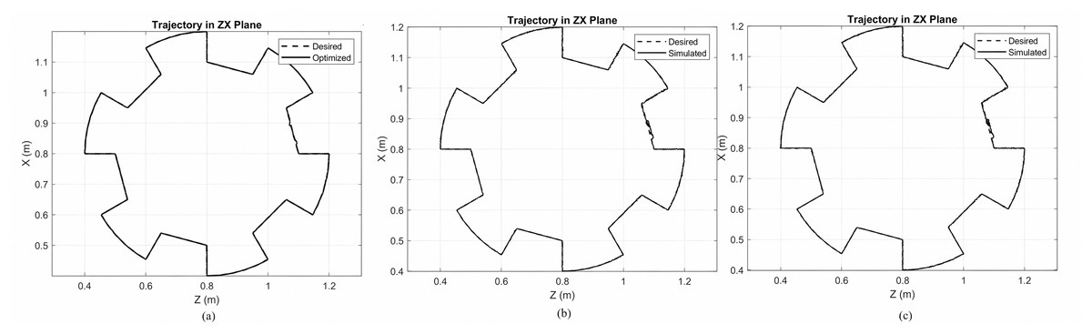
Figure 3: Simulation plots of the track of gear shape.
(A) Gear shaped path tracing for MOPSO + Lyapunov based PID controller. (B) Gear shaped path for Lyapunov based PID controller. (C) Gear shaped for PID controller.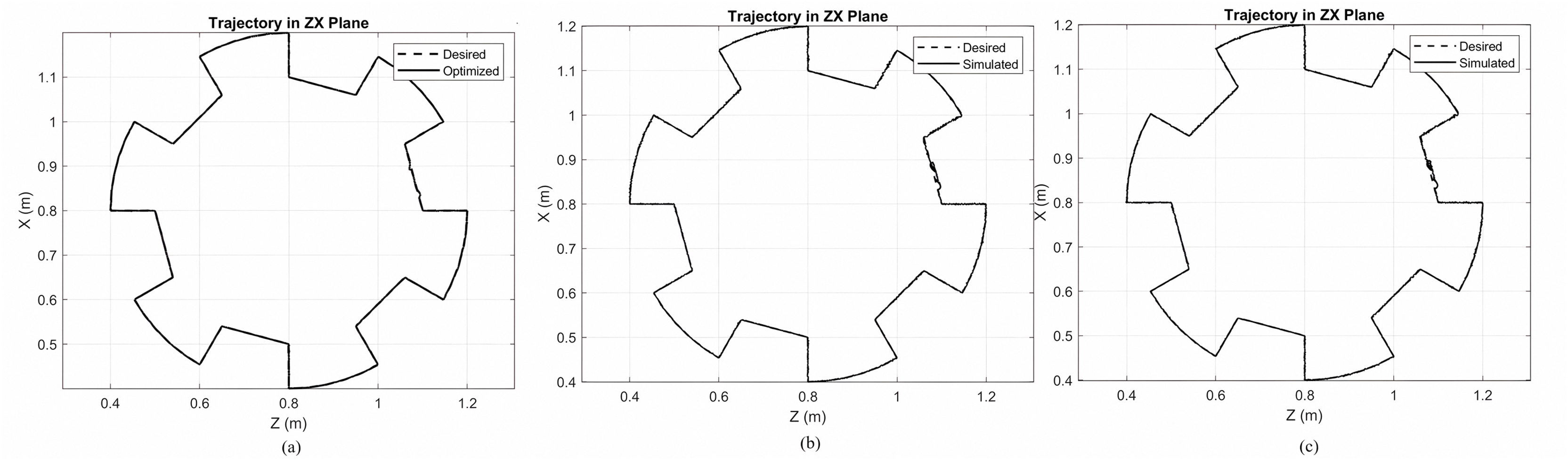
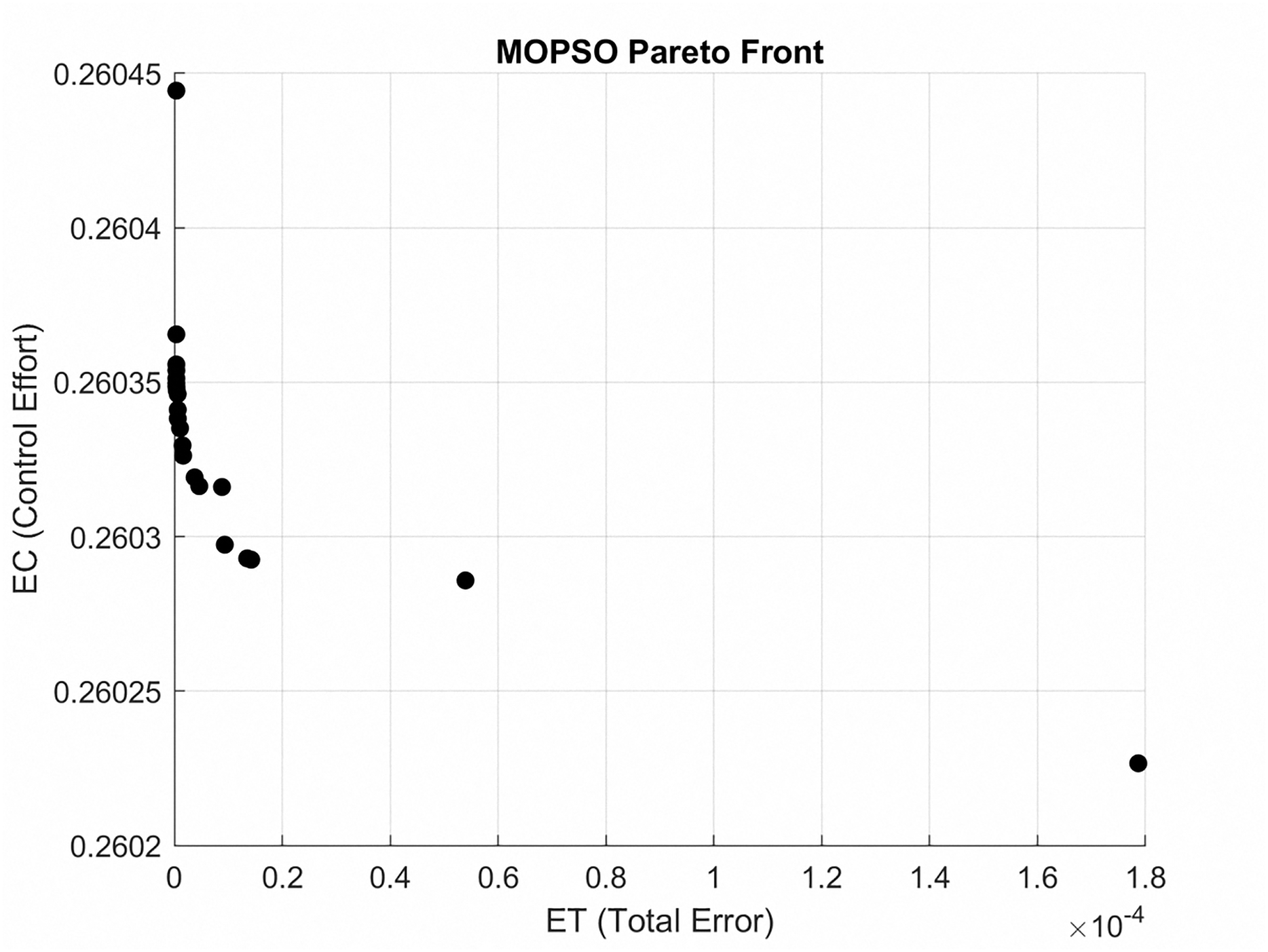
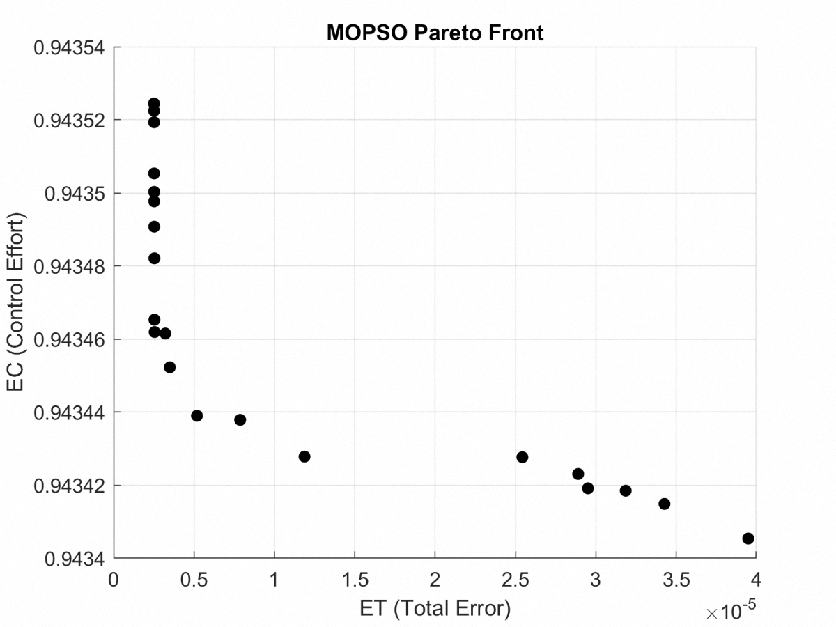
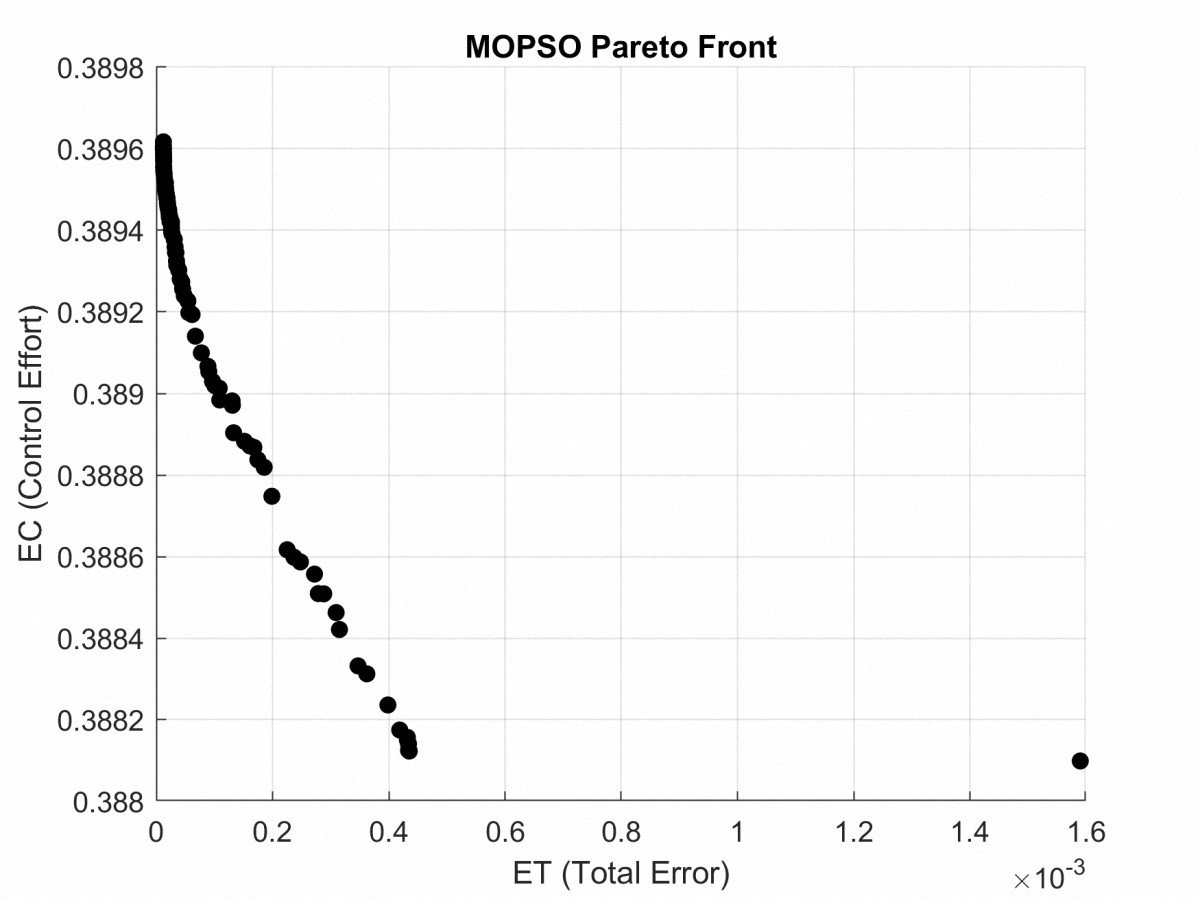
The Pareto front for the gear-shaped path is illustrated in Fig. 4. It presents the Pareto optimal trade-off between tracking error (ET) and control effort (EC) achieved through the MOPSO method. The solutions that lie within this frontier represent a range of trade-offs, allowing for flexibility based on the specific requirements of the application.
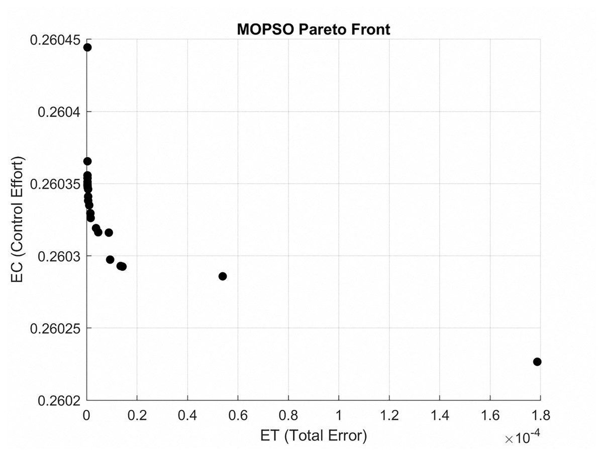
Figure 4: Pareto front for gear-shaped path, depicting Pareto trade-off between ET and EC achieved with MOPSO.
In the following descriptions the principal findings are discussed.
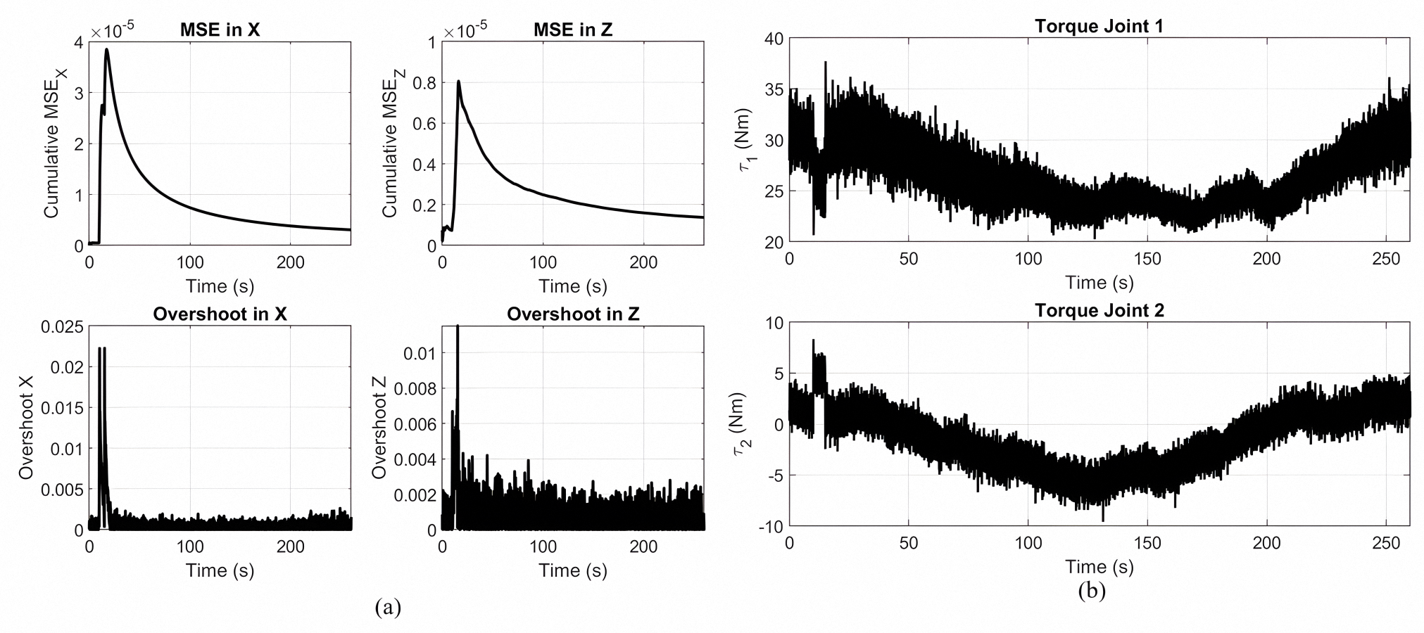
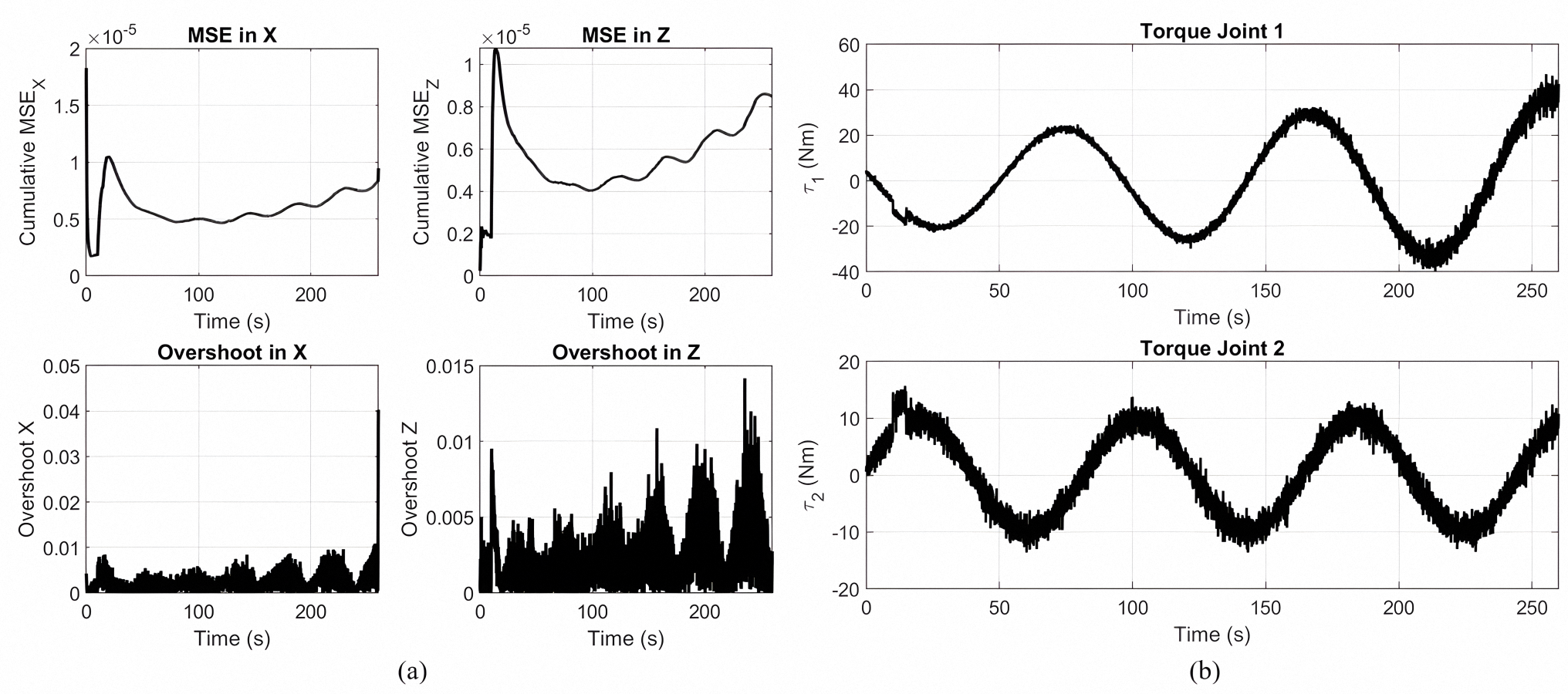
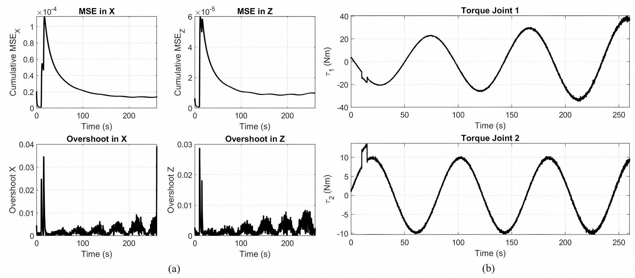
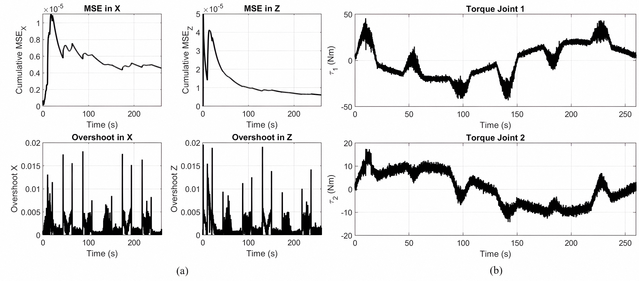
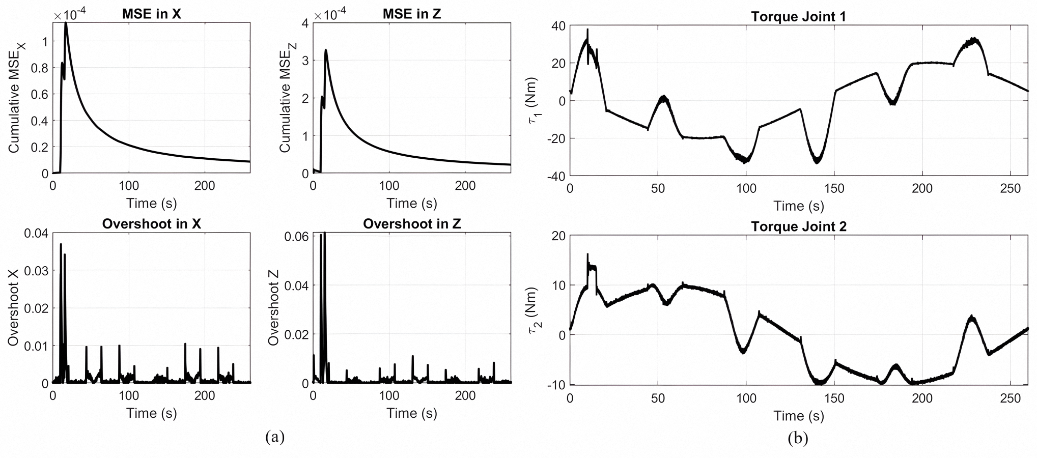
Figure 5A presents the tracking performance metrics of a gear-shaped trajectory by a Lyapunov-based PID controller optimized by MOPSO. The cumulative mean squared error in the X and Z directions, shown in the upper plots, quickly decreases and stabilizes around zero, revealing successful convergence of the trajectories. The overshoot in the X and Z directions, as shown in the lower plot, remains continuously at its lowest value, indicating high accuracy control with negligible deviation from the intended track. Figure 5B shows the Joint torque patterns for gear shaped end-effector trajectory tracking with the optimized Lyapunov PID controller. Joint 1 has larger magnitudes of the torque, in conformity to its functionality in producing the dominant motion at the end-effector, where the other Joint 2 has lower magnitudes of the torque.
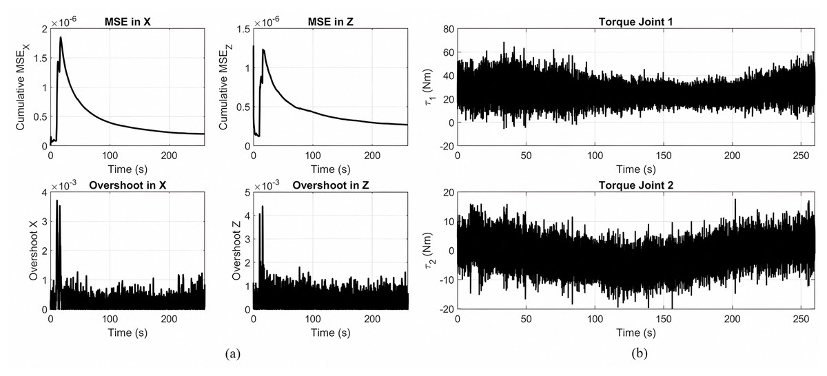
Figure 5: Principal findings.
(A) Overshoot and MSE in the X and Z directions during the tracking of a gear shaped trajectory using the optimized controller. (B) Control torques applied to each joint while following the gear-shaped path with the Lyapunov-based PID controller optimized via MOPSO.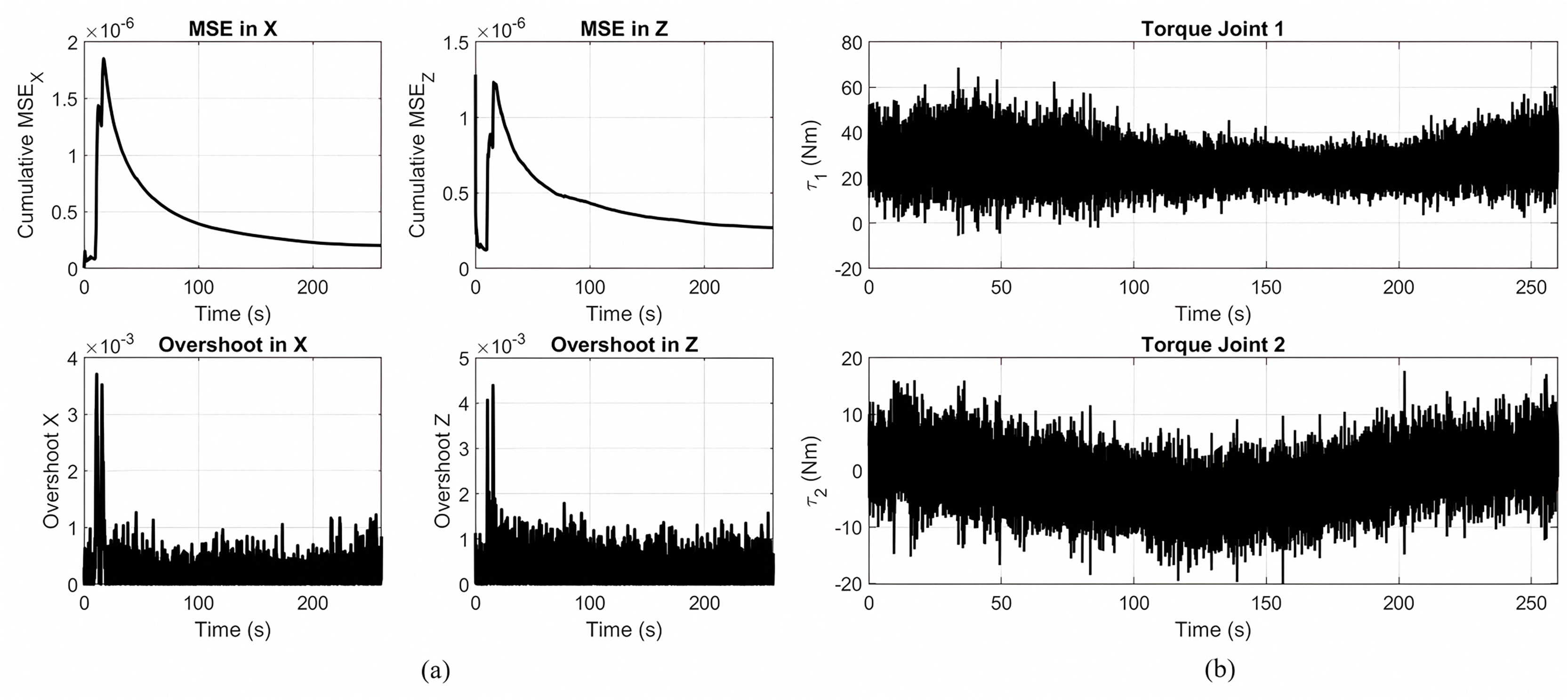
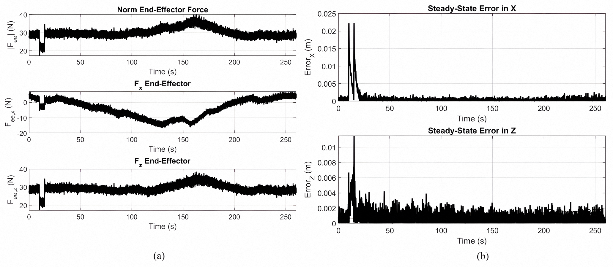
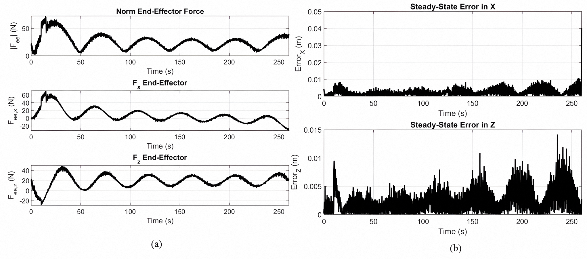
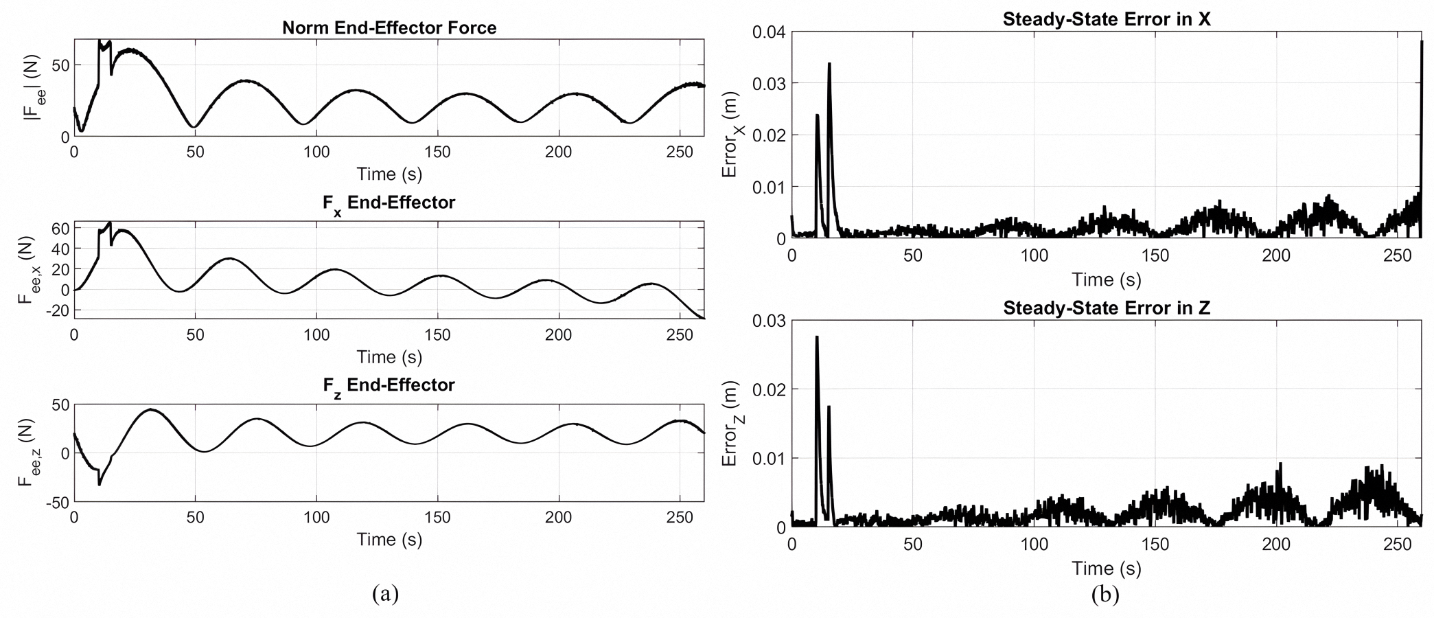
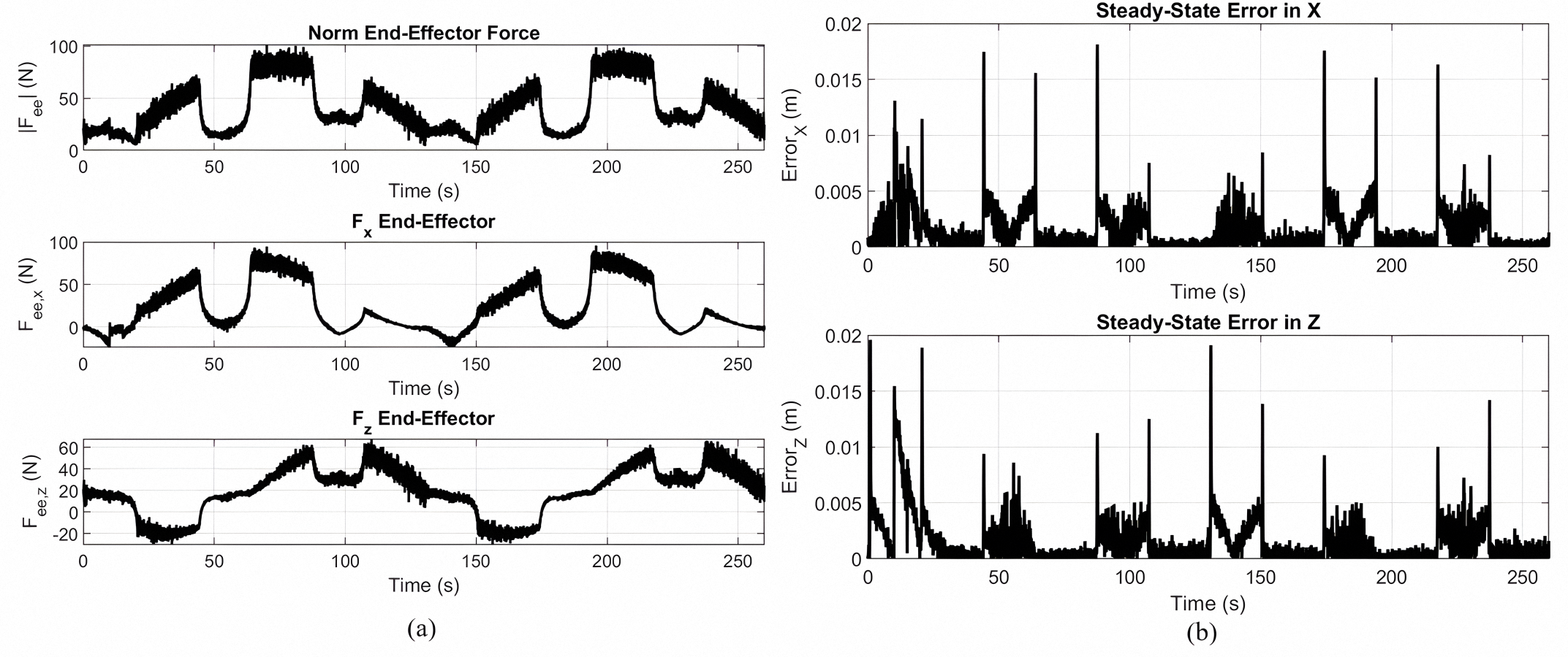
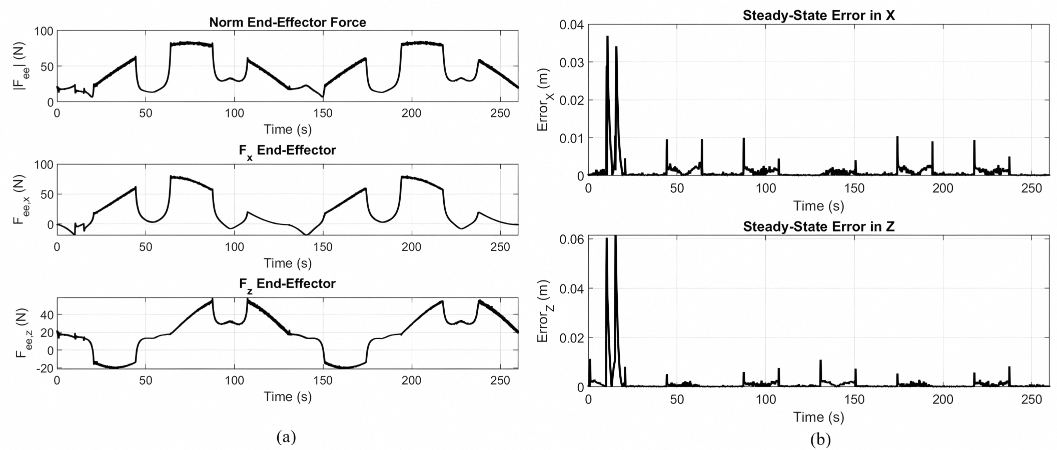
Figure 6A depicts the force response tracking the gear shaped path by the PID controller optimized by MOPSO. Top plot: the norm on the resultant end-effector force F; middle plot: the X axis components; bottom plot: the z axis components. The force magnitudes remain consistently below 50 N during the task. The force component in the X direction varies with the curved portions in the path, and the component for Z indicates vertical motion and support. The result is the stable dynamic interaction force during operation by the controller. Figure 6B depicts the steady-state tracking errors in the X and Z directions by the optimized controller for the gear shaped trajectory. Both the components of the error drop drastically when the trajectory settles down and remains on the lower side for the simulation, with excursions less than 3–4 mm. The result confirms the controller in maintaining systematic tracking errors at minimum, the evidence for its robustness and precision in sustained dynamic motion.

Figure 6: Force responses and steady-state tracking errors.
(A) Force response and (B) steady-state tracking error during gear-shaped trajectory execution using the Lyapunov-PID based controller optimized via MOPSO.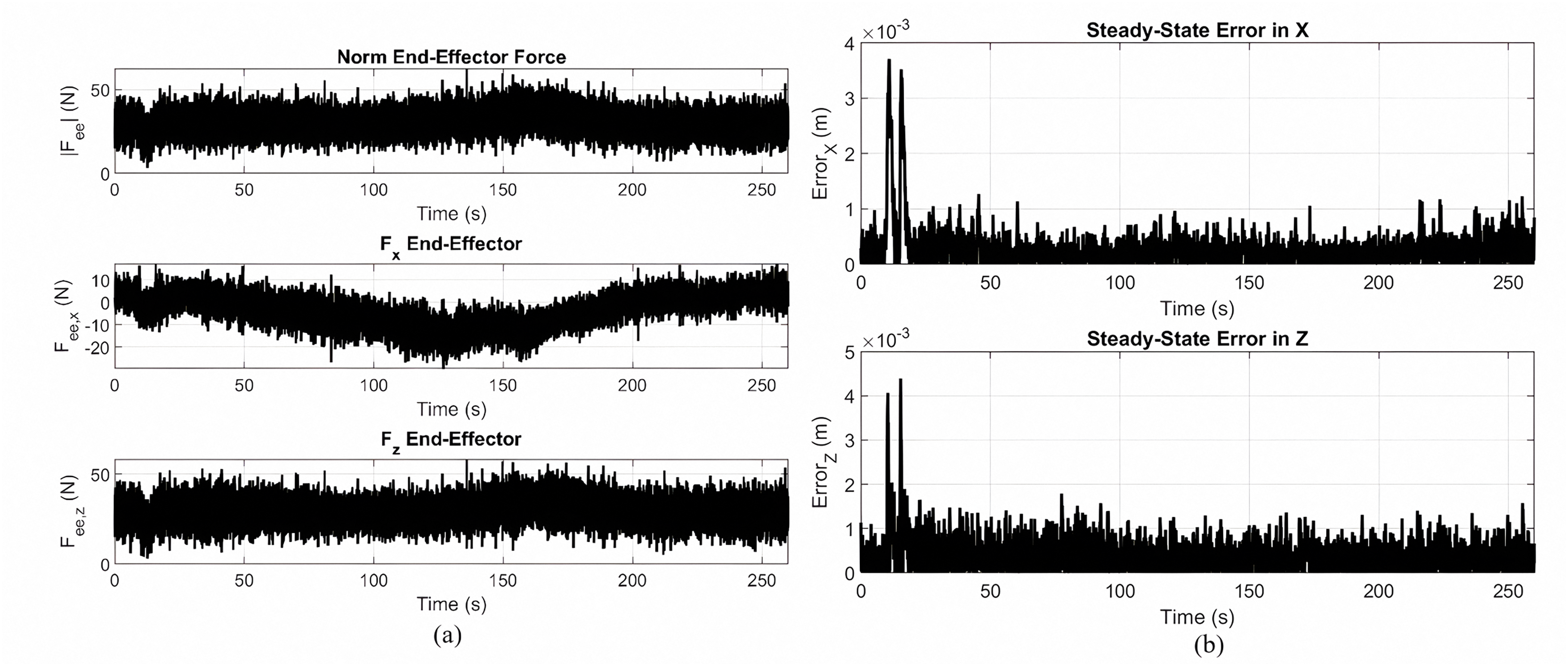
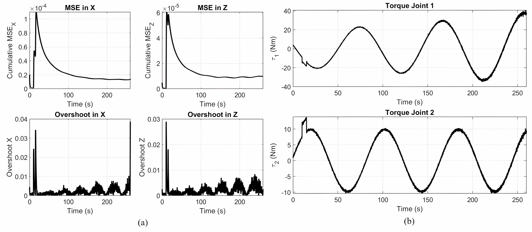
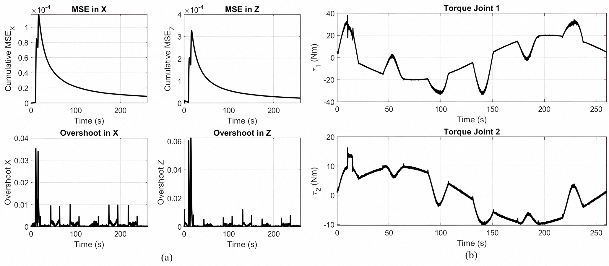
Figure 7A presents the metrics of performance during the tracking of gear shaped trajectory by the application of the Lyapunov-based PID controller in the absence of optimization. The first row depicts the cumulative MSE in the Z and X directions. The error reaches its peak and reduces gradually, indicating convergence but at a slower pace than the optimized one. The second row presents the overshooting in both directions, where it is more at the start of the trajectory and stabilizes in the later stages.
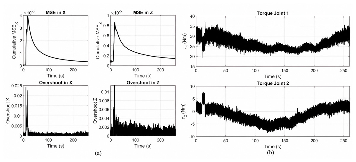
Figure 7: Metrics of performance and joint torque profiles.
(A) Cumulative MSE and overshoot in the X and Z directions during gear shape trajectory using the Lyapunov-based PID controller without optimization. (B) Joint torques applied to joint 1 and joint 2.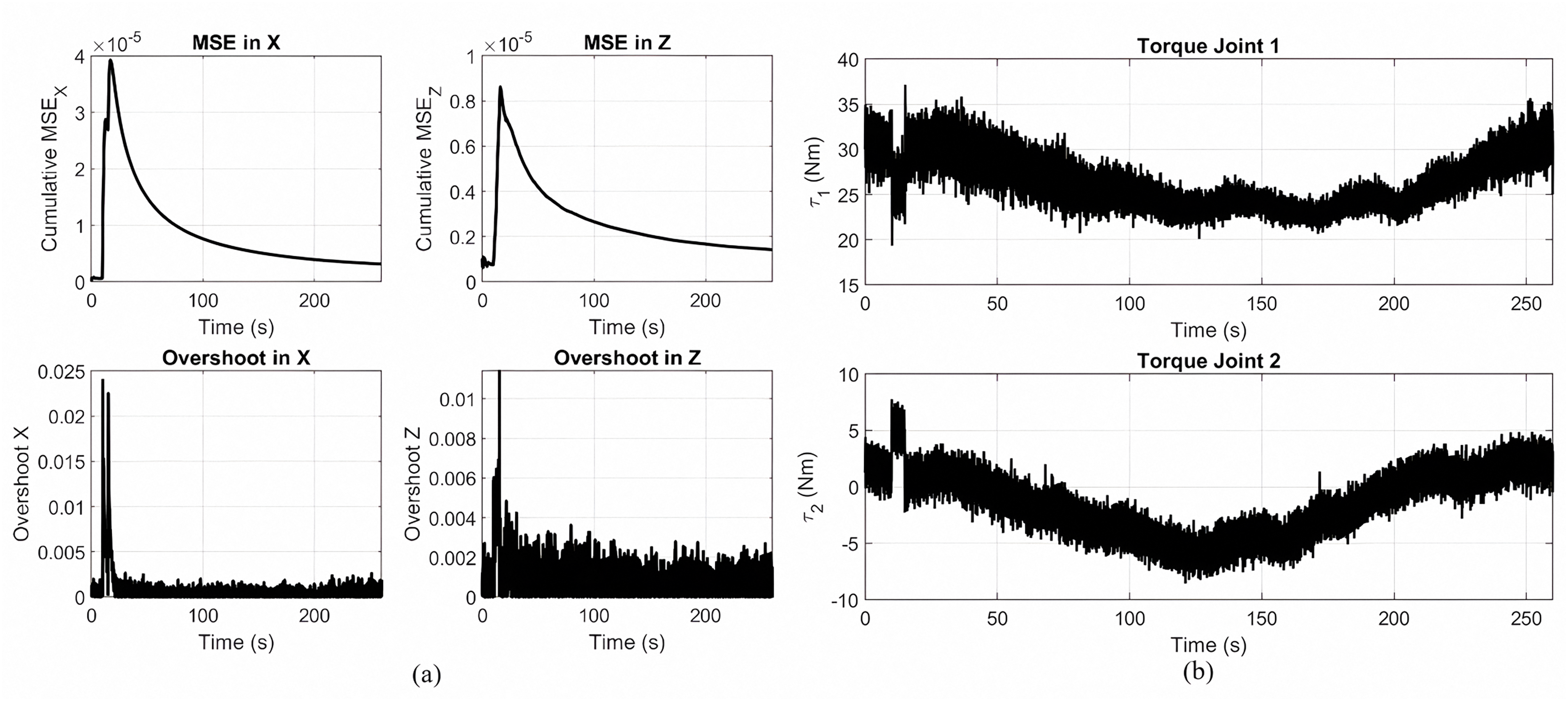
Figure 7B shows the joint torque profiles for the gear-shaped pattern with the unoptimized Lyapunov PID controller. Joint 1 has torques in the range of approximately 20 to 40 Nm, and Joint 2 is in ±10 Nm. These observations highlight the trade-off between the simplicity of the controller and its performance when tuning is not accomplished through optimization.
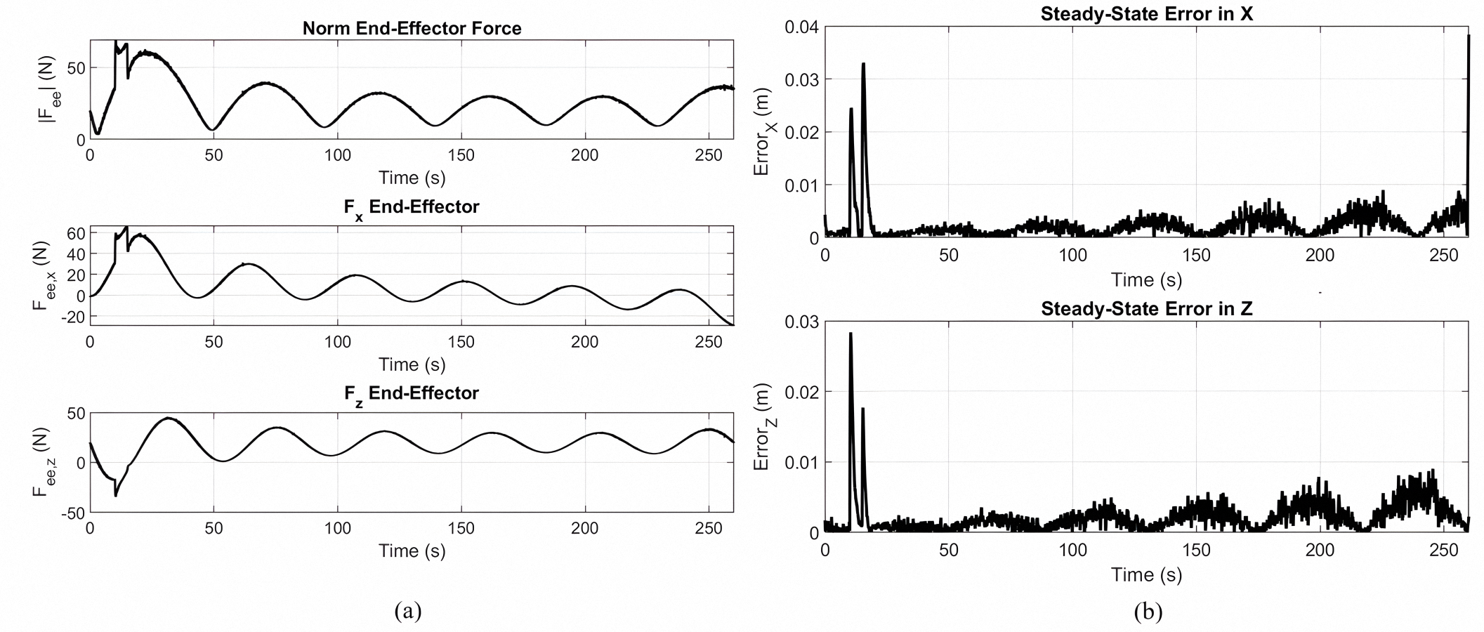
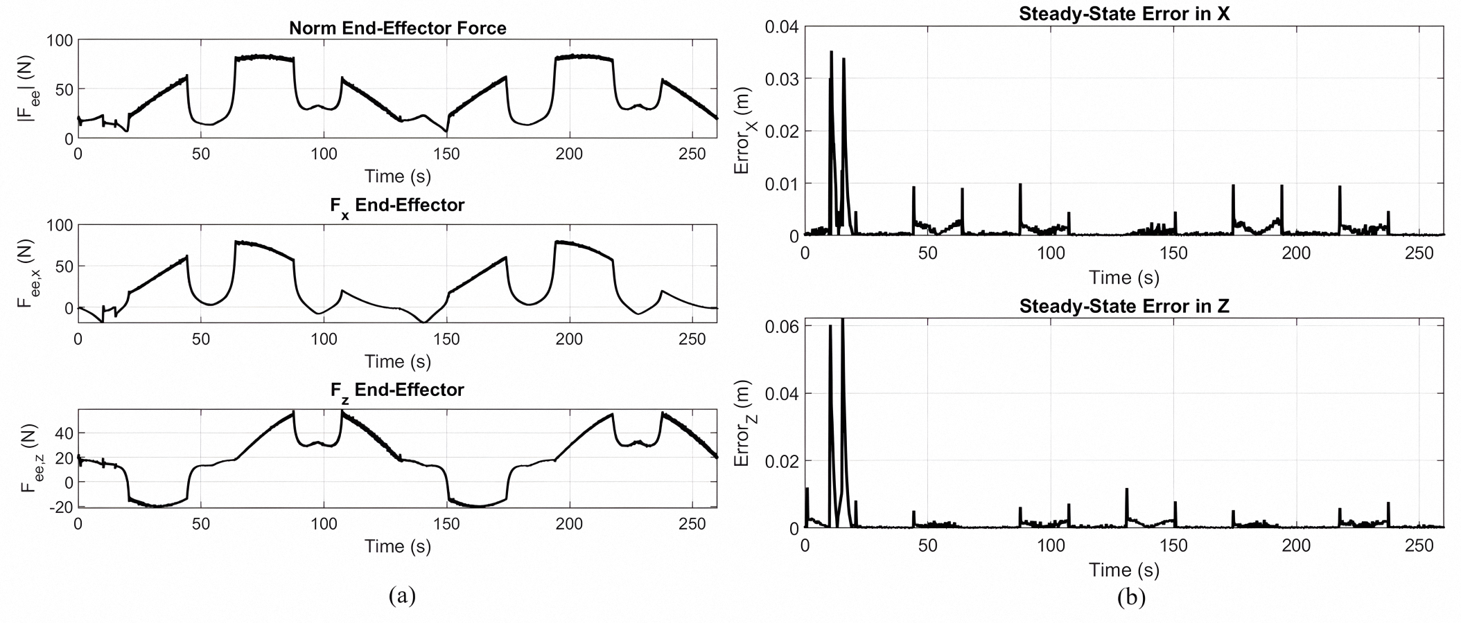
Figures 8A and 8B show the end effector force response and steady state tracking error, respectively, for the implementation of the gear-shaped trajectory by using the non-optimized version of the Lyapunov-based PID controller.
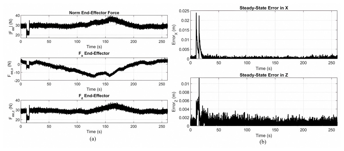
Figure 8: End effector force response and steady state tracking error.
(A) End effector response during gear shaped trajectory tracking using the Lyapunov PID controller without MOPSO. (B) Steady state tracking error in the X and Z directions.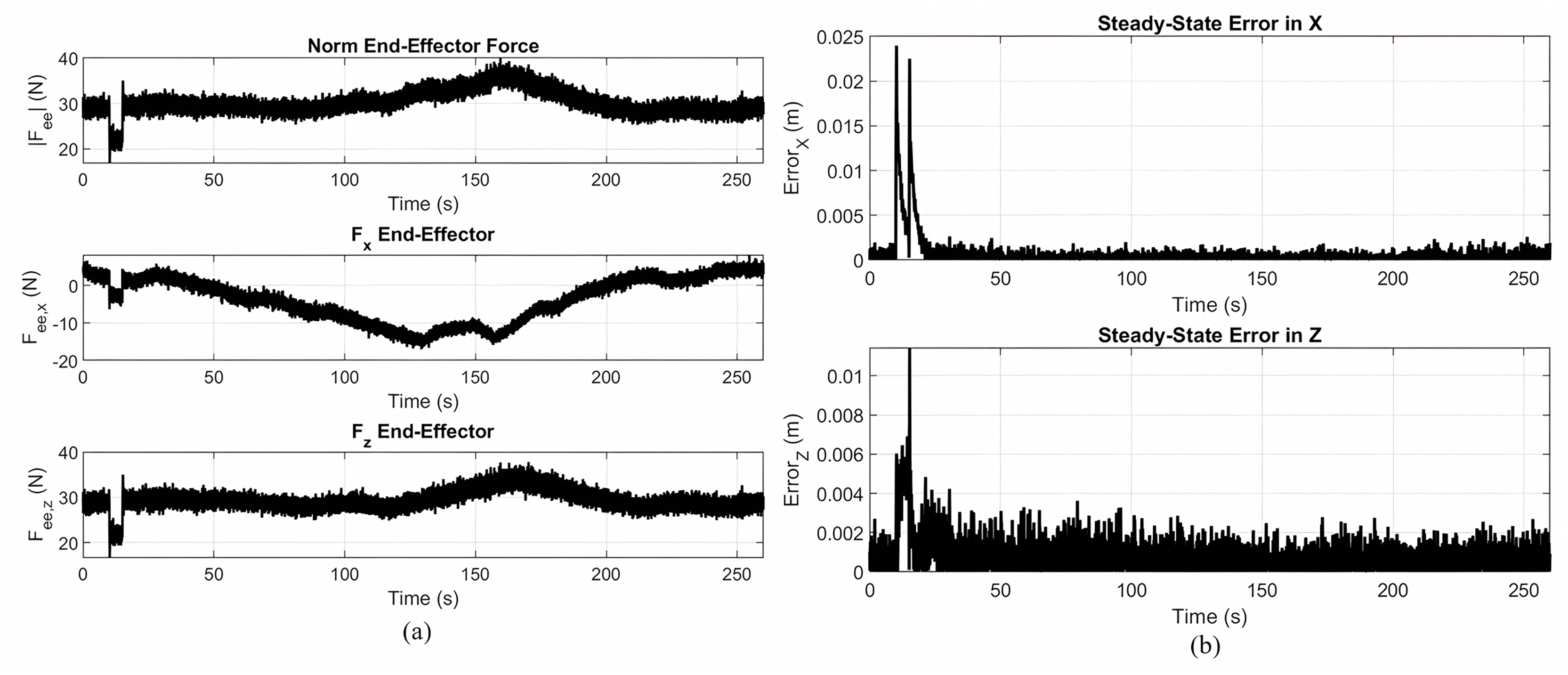
The following figures show the performance of the robotic manipulator during the tracking of a gear shaped trajectory using a classical PID controller. Figure S3A in the Supplemental Files shows the performance of the robotic manipulator during the tracking of a gear-shaped trajectory using a classical PID controller. The cumulative MSE and overshoot in the X and Z directions are presented. As seen, the tracking error starts with high peaks and gradually decreases over time. Overshoot is also more pronounced, especially during the initial moments of motion. Figure S3B in the Supplemental Files depicts the joint torques of the two actuators.
Figures S4A and S4B in the Supplemental Files present the performance of the robotic manipulator during the execution of a gear-shaped trajectory using a classical PID controller. Trajectory (a) depicts the end effector force response as a function of time. The magnitude of the total force ) oscillates between about 10 and 35 N during the task. The X component of the force oscillates between 20 and 10 N, exhibiting a distinct modulation structure which adheres to the geometry of the trajectory. Along the Z direction ( , the force oscillates between 0 N and about 30 N, exhibiting relatively consistent behavior with slight oscillations as a function of time. Figure S4B shows the steady-state tracking error along the two cartesian axes. The X error peaks at around 0.022 m during the first few seconds and has a decline, settling mainly below 0.003 m after 50 s. Analogously, the Z error peaks at around 0.007 m at the beginning and stays mainly below 0.002–0.003 m throughout the rest of the path duration.
Table 3 gives a quantitative comparison between the three considered control schemes: MOPSO optimized Lyapunov PID, non-optimized Lyapunov PID, and conventional PID for gear shape. Typical performance metrics such as steady-state error, MSE, overshoot, total control input, max torque, as well as recovery time from disturbances are provided to critically compare and evaluate each scheme’s weaknesses and strengths.
| Parameter | MOPSO-Lyapunov-PID (Optimized) | Lyapunov-PID (Non-optimized) | Traditional PID |
|---|---|---|---|
| [637, 880] | [170, 590] | [170, 590] | |
| [112.65, 131.84] | [8, 24] | [8, 24] | |
| [400, 1,450] | [65, 85] | [65, 85] | |
| Steady-state error (X (m)) | 0.00035 | 0.00061 | 0.00066 |
| Steady-state error (Z (m)) | 0.00034 | 0.00065 | 0.00068 |
| MSE_X | 2.29e−07 | 3.00e−06 | 3.10e−06 |
| MSE_Z | 3.08e−07 | 1.33e−06 | 1.32e−06 |
| Overshoot_X | 0.00383 | 0.02280 | 0.02416 |
| Overshoot_Z | 0.00441 | 0.01021 | 0.01216 |
| Total control effort (Nm∙s) | 7,669.61 | 7,548.09 | 7,547.08 |
| Max Torque Joint 1 (Nm) | 54.87 | 36.38 | 37.35 |
| Max Torque Joint 2 (Nm) | 12.88 | 8.42 | 8.74 |
| Recovery after disturbance X (s) | 0.003 | 0.020 | 0.030 |
| Recovery after disturbance Z (s) | 0.003 | 0.030 | 0.030 |
Conclusions
The comparison of three control schemes, namely optimized Lyapunov PID, non-optimized Lyapunov PID, and classical PID demonstrates that the optimized Lyapunov PID controller provides optimum overall performance. Specifically, the application of MOPSO reduces steady-state errors, mean squared errors, and overshooting considerably, and provides substantially faster recovery time after disturbance for all trajectories studied. Although the optimized method incurs slightly larger instantaneous torques and minimally larger total control work, these penalties are offset by enhanced accuracy, robustness, and response speed. Control behaviors of the non-optimized Lyapunov PID and classical PID controllers exhibit a strong similarity. They show large errors, overshooting, and significantly reduced recovery after disturbance. Such performance demonstrates the challenges that robotic control schemes face under perturbation and uncertainty and confirms the advantages of the MOPSO method. In the future work we will explore several opportunities. We will first experimentally evaluate the proposed controllers, using physical robotic equipment, and assess their performance under realistic uncertainties. We will also investigate adaptive and learning-based schemes for autotuning the gains.
Supplemental Information
Data used to generate all plots for the Gear Shape figure.
Data used to generate all plots for the Spiral Shape and Rose Curve figures.
Comparison of the control strategies in spiral trajectory tracking based on gains, overshoot, torque, and recovery time.
Gear Shape Trajectory (1).
(a) Cumulative MSE and overshoot in the X and Z directions during gear shaped trajectory using a PID controller. (b) Control torques applied to Joint 1 and Joint 2.
Gear Shape Trajectory (2).
(a) End-effector force response for gear-shaped trajectory tracking with a classical PID controller. (b) Steady-state tracking error along the X and Z axes. Maximum error reaches about 0.022 m in X and 0.007 m in Z initially, with the value remaining below 0.003 m after 50 seconds.
Spiral Trajectory (1).
(a) Spiral path tracking for MOPSO + Lyapunov-based PID controller. (b) Spiral path for Lyapunov-based PID controller. (c) Spiral for PID controller.
Spiral Trajectory (2).
(a) Cumulative MSE and overshoot in the X and Z directions during spiral trajectory tracking using a Lyapunov-PID controller optimized with MOPSO. (b) Torque signals of Joint 1 and Joint 2.
Spiral Trajectory (3).
(a) Force response for spiral path tracking of a Lyapunov-PID controller optimized using MOPSO. (b) Steady-state tracking error in the X and Z axes.
Spiral Trajectory (4).
(a) Cumulative MSE and overshoot in X and Z directions. (b) Joint 1 and Joint 2 torque profiles.
Spiral Trajectory (5).
(a) Force response of the end-effector while tracing the spiral path with the usage of a Lyapunov PID controller without MOPSO optimization. (b) Steady-state error in the X and Z directions.
Spiral Trajectory (6).
(a) Cumulative MSE and overshoot in X- and Z-directions of the classical PID controller while it tracks the spiral trajectory. The MSE decreases steadily, while the overshoot has periodic variation, large initial spikes. (b) Joint torque patterns. Periodic, regular torque signals are observed in both joints, although higher amplitude in Joint 1.
Spiral Trajectory (7).
(a) End-effector force response of the classical PID controller for tracking a spiral trajectory. The force signals are of periodic nature, high amplitude, and initial transients due to the non-optimized tuning of gains. (b) Steady state track error in the Z and X directions. The error is bounded with appreciable fluctuations in the entire track, especially at high curvature regions.
Spiral Trajectory (8).
Pareto front obtained through the MOPSO-based optimization of the Lyapunov PID controller for the aim of spiral trajectory following. The plot indicates the trade-off between control effort (EC) and overall tracking error (ET).
Rose Curve Trajectory (1).
ZX plane trajectory tracking for a rose curve with three different control strategies. (a) Optimized Lyapunov-PID controller using MOPSO with very accurate tracking and low deviation. (b) Non-optimized Lyapunov-PID controller. (c) Standard PID controller.
Rose Curve Trajectory (2).
(a) Cumulative MSE and overshoot in the X and Z directions for tracking the rose curve trajectory using the MOPSO Lyapunov PID controller. (b) Joint 1 and Joint 2 applied torque signals.
Rose Curve Trajectory (3).
(a) End-effector force response for rose curve trajectory tracking using a MOPSO optimized Lyapunov PID controller. (b) Steady state tracking error in the X and Z directions.
Rose Curve Trajectory (4).
(a) Cumulative MSE and overshoot in the X and Z directions. (b) Joint torque responses and under rose curve trajectory tracking using a Lyapunov PID controller without MOPSO optimization.
Rose Curve Trajectory (5).
(a) End-effector force norm and components during end-effector tracking of a rose curve path with a non-optimized Lyapunov PID controller. (b) Steady-state tracking errors in the X and Z axes with periodic peaks up to 0.035 m and 0.06 m, respectively.
Rose Curve Trajectory (6).
(a) Accumulative MSE and overshoot in X and Z for a rose-curve movement with a typical PID controller. (b) Joint 1 and joint 2 control torques show erratic oscillation with amplitudes as high as ±40 Nm and ±15 Nm, respectively.
Rose Curve Trajectory (7).
End-effector force components (a) and steady-state tracking error (b) for the rose curve trajectory with a PID controller.
Rose Curve Trajectory (8).
Pareto front for the rose curve path, depicting the Pareto trade-off between ET and EC achieved via MOPSO.