
Federated proximal learning with data augmentation for brain tumor classification under heterogeneous data distributions
- Published
- Accepted
- Received
- Academic Editor
- Consolato Sergi
- Subject Areas
- Artificial Intelligence, Computer Vision, Data Mining and Machine Learning, Security and Privacy, Neural Networks
- Keywords
- Federated learning, Data augmentation, Federated proximal, Privacy-preserving model training, Heterogeneous data, ResNet50 with attention head mechanism
- Copyright
- © 2025 Ghanta et al.
- Licence
- This is an open access article distributed under the terms of the Creative Commons Attribution License, which permits unrestricted use, distribution, reproduction and adaptation in any medium and for any purpose provided that it is properly attributed. For attribution, the original author(s), title, publication source (PeerJ Computer Science) and either DOI or URL of the article must be cited.
- Cite this article
- 2025. Federated proximal learning with data augmentation for brain tumor classification under heterogeneous data distributions. PeerJ Computer Science 11:e3396 https://doi.org/10.7717/peerj-cs.3396
Abstract
The increasing use of electronic health records (EHRs) has transformed healthcare management, yet data sharing across institutions remains limited due to privacy concerns. Federated learning (FL) offers a privacy-preserving solution by enabling collaborative model training without centralized data sharing. However, non-independent and identically distributed (non-IID) data distributions, where the data across clients differ in class proportions and feature characteristics, pose a major challenge to achieving robust model performance. In this study, we propose a hybrid framework that combines the Federated Proximal (FedProx) algorithm with the ResNet50 architecture to address non-IID data issues. We artificially partitioned an IID brain tumor dataset into non-IID subsets to simulate real-world conditions and applied data augmentation techniques to balance class distributions. Global model performance is monitored across 100 training rounds with varying regularization parameters in FedProx. The proposed framework achieved an accuracy of 97.71% on IID data and 87.19% in extreme non-IID scenarios, with precision, recall, and F1-scores also demonstrating strong performance. These findings highlight the effectiveness of combining data augmentation with FedProx in mitigating data imbalance in FL, thereby supporting equitable and efficient training of privacy-preserving models for healthcare applications.
Introduction
Technological advancements in healthcare have changed medical imaging of brain tumors, enhancing early and precise disease diagnosis, which is important for proper patient treatment. Among these innovations, magnetic resonance imaging (MRI)-based imaging systems have significantly improved the detection and management of critical conditions such as brain tumors. A timely detection and accurate classification of brain tumors is vital, as early detection and classification can save lives and improve patients’ quality of life. Recent advances in deep learning (DL), particularly convolutional neural networks (CNNs), have shown great potential to automate brain tumor diagnosis, reducing diagnostic delays and minimizing the dependency on expert radiologists (Oladimeji & Ibitoye, 2023; Sharif et al., 2021). However, applying DL in medical imaging, for brain tumor classification (BTC) also presents significant challenges, especially in terms of data privacy, security, and uneven distribution of patient data across institutions. Traditional DL models depend on large, centralized datasets for high performance, but patient data in medical applications is often distributed across multiple institutions. This challenge becomes even more pronounced for rare diseases and imbalanced datasets, where the limited representation of certain tumor types can bias models and compromise their generalizability. For instance, MRI datasets from different hospitals may exhibit significant disparities. One institution may have abundant glioma cases, while another predominantly stores pituitary tumor images. Such variations lead to non-IID data across institutions, posing a critical challenge in achieving equitable and robust model performance in healthcare applications.
Federated learning (FL) has become a promising approach to overcoming these challenges (McMahan et al., 2017). Unlike traditional centralized learning, FL enables collaborative model training across distributed datasets by transmitting only model updates to a central server, ensuring patient data remain local. The most widely adopted baseline in FL is the Federated Averaging (FedAvg) algorithm, which aggregates locally trained model updates from clients to build a global model without requiring the sharing of raw data. Although FL improves privacy and security, it introduces new challenges related to non-IID data. Real-world variations in data collection and storage can exacerbate dataset imbalances, negatively impacting global model performance. Addressing these limitations requires strategic methods to balance data distribution and optimize model training. Most existing studies on FL for medical imaging have been conducted on datasets that are either IID (Albalawi et al., 2024; Islam et al., 2023) or only mildly non-IID (Viet et al., 2023), which do not fully capture the extreme divergence often encountered in real-world clinical settings. In practice, certain institutions may contribute datasets that are heavily skewed toward specific tumor types, resulting in highly imbalanced local data distributions. This extreme label-skew scenario represents a particularly challenging form of non-IID data, which can significantly hinder convergence and degrade global model accuracy, yet it remains underexplored.
Motivated by these challenges, our study proposes a structured methodology that integrates data augmentation with the Federated Proximal (FedProx) algorithm to address data imbalance in FL for BTC using MRI images. Data augmentation is employed to create more balanced client datasets, ensuring equitable representation of tumor classes (Perez & Wang (2017). FedProx (Li et al., 2020), an extension of FedAvg, mitigates the adverse effects of heterogeneous client data by introducing a proximal term in the optimization process. This reduces client model divergence and enhances global model performance. By combining FedProx with data augmentation, our work aims to improve the robustness and accuracy of federated BTC models under realistic and highly non-IID conditions. To further enhance classification performance, we adopt transfer learning integrated with dual-pooling attention mechanism. Various transfer learning architectures are evaluated, and ResNet50 is selected as the backbone based on its superior performance. The fine-tuned ResNet50 model with FedProx regularization was rigorously evaluated using multiple performance metrics to ensure comprehensive assessment.
By addressing dataset imbalances and enhancing fairness in FL, our work seeks to explore how FL can effectively handle non-IID medical datasets to build privacy-preserving and unbiased models for BTC. Our findings highlight the potential of FL to integrate distributed healthcare data into robust artificial intelligence (AI)-based solutions, thus advancing intelligent and equitable healthcare systems. The source code for all conducted experiments is available in our GitHub repository at https://github.com/Sumanth-Siddareddy/FederatedProximal.
Contributions
The main contributions of this study are as follows:
integration of a dual-pooling attention mechanism within a Residual Network-50 (ResNet50) backbone under an FL framework
integration of clinically constrained data augmentation to address non-IID medical data
incorporation of the FedProx algorithm to enhance convergence stability and model robustness under extreme label skew scenarios
extensive experimental validation demonstrating improved generalization compared to existing FL methods
The remainder of this article is structured as follows. The Related Work section reviews existing literature and groups prior studies thematically. The Methods section describes the data splitting strategy, the FL algorithms considered (FedAvg and FedProx), model selection, and the data augmentation strategies employed. The Results section presents the experimental findings, while the Discussion section provides a detailed analysis and interpretation of these results. Finally, the Conclusion and Future Work sections summarize the study and outline potential directions for future research.
Related work
Deep learning for brain tumor classification
Many studies have leveraged DL models for BTC using centralized datasets. Fathima & Kumar (2024) applied transfer learning with VGG, InceptionV3, and DenseNet201 for BTC, achieving 94.73% accuracy with Visual Geometry Group (VGG). Model performance improved over 25 epochs, but dataset limitations from Kaggle may impact generalizability. Senan et al. (2022) introduced a hybrid model combining DL (AlexNet, ResNet-18) with machine learning (SVM) for early brain tumor diagnosis. Achieving a 95.10% accuracy, the approach effectively classifies MRI images while enhancing sensitivity (95.25%) and specificity (98.50%). However, larger and more diverse datasets are essential for better generalization, highlighting the need for advanced augmentation techniques and real-world clinical validation to improve practical applicability. Sharif et al. (2021) developed an automated DL system using Densenet201 and novel feature selection techniques, Entropy-Kurtosis-based High Feature Values (EKbHFV), and a modified genetic algorithm (MGA) for multiclass BTC. Achieving over 95% accuracy, the method demonstrates high precision with the Cubic SVM classifier on the BRATS2018 and BRATS2019 datasets. However, challenges persist in distinguishing similar tumor types and managing high-dimensional datasets. Vidyarthi et al. (2022) introduced a machine learning-assisted methodology for multiclass classification of high-grade malignant brain tumors, utilizing the novel Cumulative Variance Method (CVM) for feature selection. Nazir et al. (2024) introduced a customized CNN model for brain tumor prediction using MRI images, integrating Explainable AI (XAI) techniques such as SHapley Additive exPlanations (SHAP), Local Interpretable Model Agnostic Explanation (LIME), and Gradient-weighted Class Activation Mapping (Grad-CAM) to enhance model interpretability, achieving an accuracy of 94.64%. These studies demonstrate the effectiveness of DL methods in tumor segmentation but also highlight challenges such as class imbalance and limited data availability.
Class imbalance and rare tumor types
Deepak & Ameer (2023) on BTC overcomes dataset imbalance using class-weighted focal loss and deep feature fusion, achieving 95.4% accuracy. Majority voting on classifier predictions further enhanced performance. However, optimizing class weights remains a challenge, potentially leading to biased predictions. The research employs K-nearest neighbor (KNN), multi-class support vector machine (mSVM), and neural network (NN) classifiers, achieving a peak accuracy of 95.86% with NN. While the method improves classification precision, gaps remain in studying rare malignant tumors and incorporating DL approaches for enhanced performance. Khan et al. (2022b) employed a 23-layer CNN and fine-tuned Visual Geometry Group 16 (VGG16) for binary and multiclass brain tumor detection, achieving 97.8% accuracy on a Figshare dataset and 100% accuracy on a smaller dataset. Despite high performance, limitations include the lack of clinical data validation and challenges in acquiring annotated images, raising concerns about overfitting and dataset diversity.
Federated learning for privacy-preserving brain tumor classification
To overcome data-sharing restrictions in medical imaging, recent studies have explored FL. A survey by Podschwadt et al. (2022) examined DL architectures for privacy-preserving machine learning (PPML) using fully homomorphic encryption (HE), highlighting computational overhead and usability challenges. They explored techniques such as polynomial approximations and FL. However, interoperability issues, encryption complexity, and performance trade-offs remain key limitations. Talukder, Islam & Uddin (2023) introduces an optimized ensemble DL model for BTC, achieving 91.05% (with FL) and 96.68% (without FL) accuracy using Grid Search-based Weight Optimization (GSWO). The research enhances workflow efficiency through image standardization, pre-processing, and transfer learning modifications, while weight optimization techniques, like GSWO, refine predictive accuracy. The study Zhou, Wang & Zhou (2024) on FL for MRI brain tumor detection ensures data privacy while improving diagnostic accuracy. Using the FedAvg algorithm and EfficientNet-B0, the model achieved an 80.17% accuracy across diverse datasets, outperforming existing methods. However, challenges such as data heterogeneity and institutional variability affect generalization, requiring advanced model designs for improved interpretability. Ay, Ekinci & Garip (2024) explores FL for MRI-based BTC while preserving data privacy. By evaluating FedAvg, QFedAvg, Ft-FedAvg, and Dp-FedAvg, the research highlights FedAvg’s superior accuracy (85.55% at 10 rounds) and Ft-FedAvg’s robustness (85.80% at 30 rounds). However, the assumption of balanced data sharing and reliance on centralized communication limits real-world applicability.
Federated learning under non-IID data
Some studies have considered FL under non-IID scenarios, such as Viet et al. (2023), but did not provide details about the data splitting strategies or how they managed the non-IID nature of the data. Another work by Zhang et al. (2023) applied data augmentation to mitigate data heterogeneity in FL. Although this approach effectively increased the number of samples in each client, it did not address the extreme divergence scenario between the client and global models, which limited the overall generalization performance.
Our proposed work effectively addresses the limitations and research gaps identified in previous studies on BTC using DL and FL. While prior works struggled with data heterogeneity, class imbalance, and limited generalization across diverse datasets, our approach mitigates these challenges by integrating advanced data augmentation techniques and employing the FedProx algorithm. Unlike studies that relied on static weight optimization or conventional aggregation methods, our use of FedProx enhances model robustness by adapting to non-IID data distributions, ensuring improved generalization across fragmented healthcare datasets. In addition to FedProx, alternative federated optimization methods such as FedNova (Wang et al., 2020) and FedOpt (Reddi et al., 2020) have been proposed. FedNova primarily addresses the challenge of heterogeneous local training effort by normalizing client updates when clients perform varying numbers of local steps.
Since our experimental setup considered uniform local training across clients, the benefits of FedNova would be limited in our setting. FedOpt, on the other hand, employs adaptive server-side optimizers to stabilize and accelerate convergence. Although valuable for improving optimization dynamics, they do not directly mitigate client drift arising from highly skewed label distributions, which is the central challenge in our work. We therefore focused on FedProx, which explicitly introduces a proximal term to control drift under non-IID data, making it particularly suitable for our extreme label-skew scenario, providing a more practical and scalable solution for real-world clinical applications.
Methods
In this experimental study, we address the challenges posed by non-IID data in BTC using an FL approach. The primary focus is on the FedProx algorithm, which aims to enhance model performance under non-IID data conditions. This study is particularly significant as it explores the integration of data augmentation techniques to create more uniform data distributions, a crucial step toward improving the robustness of machine learning models in medical applications.
Data preparation
Dataset: The dataset used in this work comprises 7,023 brain MRI images categorized into four classes: glioma, meningioma, pituitary, and no tumor. These images are obtained from the publicly available Brain Tumor MRI dataset on Kaggle (Nickparvar, 2021). This dataset is formed by combining three widely used brain tumor MRI datasets such as Br35H, Figshare, and SARTAJ Figshare to provide a more comprehensive and diverse collection of MRI scans (Ghanta et al., 2025a).
Non-IID data partitioning and heterogeneity quantification
The dataset was initially in an independent and identically distributed (IID) format, and Table 1 represents the data distribution of the original dataset. To simulate a realistic and challenging extreme label-skew FL scenario, we partitioned the dataset across four clients using a majority-class label-skew non-IID splitting strategy. This setup mimics a real-world scenario where each client (e.g., a hospital) specializes in a particular tumor type.
| Class | Training samples | Testing samples |
|---|---|---|
| Glioma | 1,321 | 300 |
| Meningioma | 1,339 | 306 |
| No tumor | 1,595 | 405 |
| Pituitary | 1,457 | 300 |
Splitting strategy
Each of the four clients is assigned a majority of images from one of the four classes (glioma, meningioma, notumor, pituitary) and a small, fixed number of samples from the other three classes. For example, out of 1,321 training images, Client 1 receives 1,021 images, while the remaining three clients receive 100 images each. This manual assignment strategy has resulted in a non-IID setup, as detailed in Table 2. The specific images for each client’s partition are then selected randomly from the main dataset’s pools. To ensure our experimental setup is fully reproducible, a fixed seed (random_state=42) is used during this sampling process.
| Class | Client 1 | Client 2 | Client 3 | Client 4 |
|---|---|---|---|---|
| Glioma | (1021, 210) | (100, 30) | (100, 30) | (100, 30) |
| Meningioma | (100, 32) | (1039, 210) | (100, 32) | (100, 32) |
| No tumor | (100, 50) | (100, 50) | (1295, 255) | (100, 50) |
| Pituitary | (100, 50) | (100, 50) | (100, 50) | (1157, 150) |
Quantification of data heterogeneity
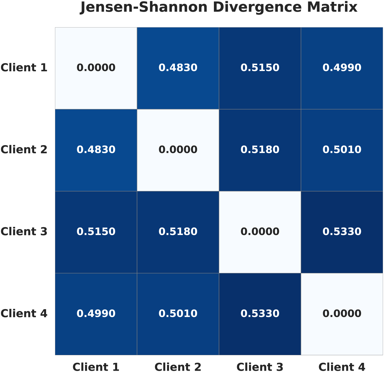
To formally quantify the degree of non-IID heterogeneity, we calculated the Jensen-Shannon (JS) divergence (Nielsen, 2020) between the label probability distributions of each pair of clients. For each client, the label distribution is defined as the proportion of samples belonging to each class. The pairwise JS divergence values are visualized as a heatmap in Fig. 1. Higher values in the heatmap indicate greater statistical distance between client datasets, and thus stronger non-IID heterogeneity. This provides an objective measure of the heterogeneity introduced by our data splitting strategy.

Figure 1: Jensen-Shannon divergence matrix of the four clients in the non-IID setup.
FL and the challenge of data heterogeneity
FL is a machine learning paradigm that enables multiple decentralized devices or institutions (clients) to collaboratively train a global model without sharing their private local data. This approach is particularly beneficial in domains like healthcare, where data privacy and security are paramount. One of the significant challenges in FL is data heterogeneity, where the data distributions across clients are non-IID. This heterogeneity can lead to discrepancies in local model updates, making it difficult to train a robust global model that generalizes well across all clients.
Federated averaging (FedAvg)
FedAvg is the foundational algorithm for FL. It operates through an iterative process involving the following steps:
-
•
Initialization: A central server initializes a global model and shares it with all participating clients.
-
•
Local training: Each client updates the global model using its local data for a specified number of epochs. This process involves computing gradients based on the client’s local loss function and adjusting the model weights accordingly.
-
•
Model weight Upload: After local training, clients send their updated model weights back to the central server.
-
•
Aggregation: The central server aggregates the received updates to form a new global model. In FedAvg, this aggregation is typically a weighted average of the clients’ models, with weights proportional to the size of each client’s dataset. (1) where:
-
–
: Model weights on client at iteration
-
–
: Learning rate
-
–
: Gradient of the loss function for client (2)
-
–
K: Total number of clients
-
–
: Number of data points on client
-
–
: Total number of data points across all clients
-
-
•
Iteration: Steps—Local training, model weight upload, and aggregation—are repeated for multiple rounds until the global model converges or achieves satisfactory performance.
FedAvg is a straightforward approach that serves as a baseline for FL methods. However, it assumes IID local data and can perform poorly when client data is highly non-IID (McMahan et al., 2017).
Federated proximal (FedProx)
To address the limitations of FedAvg in the presence of data heterogeneity, the FedProx algorithm was introduced. FedProx builds upon FedAvg by modifying the local objective function to include a proximal term, which helps stabilize training when the client data distributions are vastly different. The steps of the FedProx algorithm are outlined below:
-
•
Initialization: The central server initializes the global model and shares it with all clients.
-
•
Local training with proximal term: Clients perform local model updates by minimizing their augmented local objective function, which includes the proximal term. (3) where:
-
–
: Local loss function on client
-
–
: Current local model weights
-
–
: Global model weights from the server
-
–
: proximal term
-
–
: Proximal regularization parameter
-
-
•
Model upload: Clients send their updated model parameters back to the server.
-
•
Aggregation: The server aggregates the models using a weighted average, similar to FedAvg.
-
•
Iteration: Repeat the above steps for multiple rounds.
The proximal term mitigates the impact of local updates diverging too far from the global model, which is common under non-IID data. The proximal regularization parameter (or mu) controls the strength of this proximal term, thereby limiting drastic deviations in local updates that could negatively impact the global model when the updates are aggregated. By adjusting the regularization parameter , FedProx allows control over the trade-off between local optimization and adherence to the global model. A higher value of places more emphasis on the proximal term, causing local models to remain closer to the global model. This can be beneficial when data heterogeneity is high. A lower reduces the impact of the proximal term, allowing local models to optimize more freely based on their local data. Selecting an appropriate is crucial and often requires empirical tuning based on the specific dataset and degree of non-IID-ness (Li et al., 2020). FedProx promises better convergence properties in heterogeneous environments compared to FedAvg.
Differences between FedAvg and FedProx
In FedProx, the value acts as a regularization parameter to control the divergence between local models and the global model. For example, setting adds a proximal term to the loss function, penalizing local updates that deviate significantly from the global model, while reduces FedProx to the standard FedAvg algorithm. FedAvg works well when client data distributions are IID and computational capabilities are uniform. FedProx is designed for non-IID settings and client heterogeneity by adding the proximal term to the local objective, which restricts the extent to which local models diverge from the global model. Table 3 summarizes some main differences between FedAvg and FedProx.
| FedAvg | FedProx |
|---|---|
| 1. Fewer parameters, simpler tuning, and faster to implement | 1. Requires tuning of the proximal regularization parameter ( ) |
| 2. Computationally efficient | 2. Increased computational cost |
| 3. No proximal term, performs standard averaging of client updates | 3. Adds a proximal term and improves stability in convergence under heterogeneity |
| 4. Less robust and performance can degrade with non-IID (heterogeneous) data | 4. More stable local updates and handles non-IID data better due to the proximal term |
| 5. May diverge in heterogeneous settings | 5. Better at handling divergence issues |
Model selection
In this research, we selected transfer learning approaches such as ResNet50, VGG19, ResNet18, MobileNetV2, and Efficient-B0 models with an attention module, as they are well-suited for the BTC problem. These models are known for their strong capability in pattern recognition within medical images (Ghanta, Thiriveedhi & Pradhan, 2024), making them effective choices for this task. ResNet models help process deep features efficiently, while VGG19 provides a structured approach for learning important details. The attention mechanism further improves the focus on tumor regions, ensuring better accuracy even with diverse data in an FL setup. We provide a brief discussion of these models below.
ResNet50
ResNet50 is a deep CNN with a 50-layer architecture, introduced as part of the Residual Network (ResNet) family by He et al. (2016). The key innovation of ResNet is the introduction of residual learning through skip connections or shortcut connections, which help mitigate the problem of vanishing gradients in very deep networks. The significance of it is that, by using residual connections, ResNet50 alleviates the degradation problem found when training deep networks. It achieved state-of-the-art results on the ImageNet dataset, winning the ImageNet Large Scale Visual Recognition Challenge (ILSVRC) in 2015. It is widely used as a backbone in various computer vision tasks due to its strong feature extraction capabilities (Veeramreddy et al., 2024).
ResNet18
ResNet18 is another architecture from the ResNet family, with an 18-layer architecture. Utilizes Basic residual blocks with two layers each. It is characterized by fewer parameters, lower computational requirements, and shallower depth compared to ResNet50. It is suitable for applications with limited computational resources or where faster inference is required and is often used as a benchmark model to evaluate new techniques due to its simplicity (Tang & Teoh, 2023).
VGG19
VGG19 is a deep CNN model, part of the VGG architectures developed by Simonyan & Zisserman (2014), with a 19-layer architecture. Uses small 3 3 convolutional filters throughout the network. Consists of sequential convolutional layers followed by max pooling layers, culminating in fully connected layers. It achieved top results in the ILSVRC 2014 competition, and its significance lies in the use of small, consistent convolutional filters, which makes the architecture straightforward to implement and understand. Pre-trained versions of VGG19 are widely used for transfer learning in various image recognition tasks (Simonyan & Zisserman, 2014).
MobileNetV2
MobileNetV2 is a lightweight CNN architecture designed for efficient performance on mobile and embedded devices, introduced by Howard et al. (2017). Its core innovation lies in the use of inverted residual blocks with linear bottlenecks, which significantly reduce the computational cost while preserving representational power. This design enables MobileNetV2 to achieve a good balance between accuracy and efficiency, making it suitable for real-time applications where resources are constrained. It has been widely adopted as a backbone for tasks such as image classification, object detection, and semantic segmentation due to its fast inference speed and low parameter count (Ghanta et al., 2025b).
EfficientNet-B0
EfficientNet-B0 is the baseline model of the EfficientNet family, proposed by Tan & Le (2019), which introduced a novel compound scaling method to uniformly scale depth, width, and resolution of CNNs. Unlike prior models that scale these dimensions arbitrarily, EfficientNet applies a principled approach that leads to better accuracy and efficiency trade-offs. EfficientNet-B0, in particular, achieves strong performance on ImageNet while requiring significantly fewer parameters and FLOPs compared to earlier architectures. Its efficiency and scalability make it a popular backbone for a wide range of computer vision tasks.
Impact of model architecture on performance
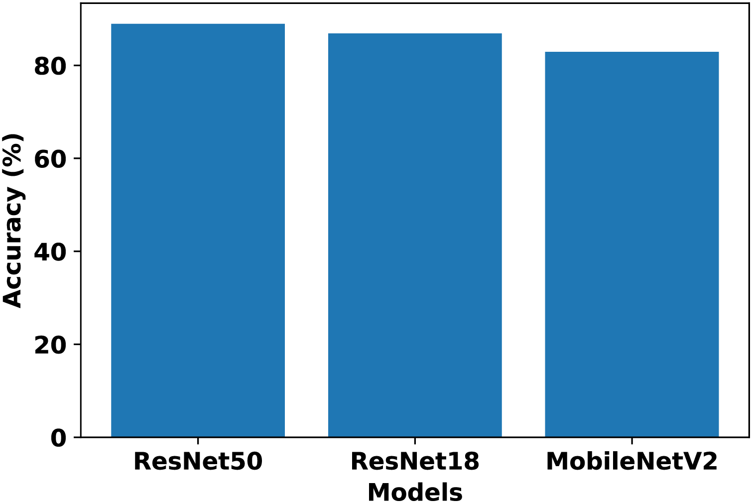
In our work, we consider these model architectures to evaluate their suitability for BTC in an FL setup. Each client is trained on its respective non-IID dataset using the above architectures to determine standalone performance. The chosen architectures represent a range of complexity levels commonly used in image classification tasks. Comparing the results across four clients, ResNet50 achieved the highest standalone performance, while ResNet18 and MobileNetV2 had competitive results. VGG19 and EfficientNet-B0 trailed in both accuracy and F1-score. Table 4 presents the performance metrics of each client across model architectures. Based on these results, ResNet50, ResNet18, and MobileNetV2 are selected for further evaluation in the FL setup, whereas VGG19 and EfficientNet-B0 are excluded due to their relatively lower performance. After comparing the FedAvg results of FL from Fig. 2, ResNet50 is selected as the most suitable model for our FL setup.
| Model | Client 1 (%) | Client 2 (%) | Client 3 (%) | Client 4 (%) | Avg. (%) | Avg. F1_score |
|---|---|---|---|---|---|---|
| ResNet50 | 88.63 | 72.39 | 62.85 | 80.47 | 76.09 | 0.7588 |
| ResNet18 | 75.82 | 70.86 | 65.37 | 84.59 | 74.16 | 0.7319 |
| VGG19 | 77.04 | 61.40 | 69.41 | 70.25 | 69.53 | 0.6467 |
| MobileNetV2 | 84.36 | 62.47 | 73.30 | 80.47 | 75.15 | 0.7395 |
| EfficientNet-B0 | 67.58 | 67.35 | 60.26 | 62.62 | 64.45 | 0.5998 |
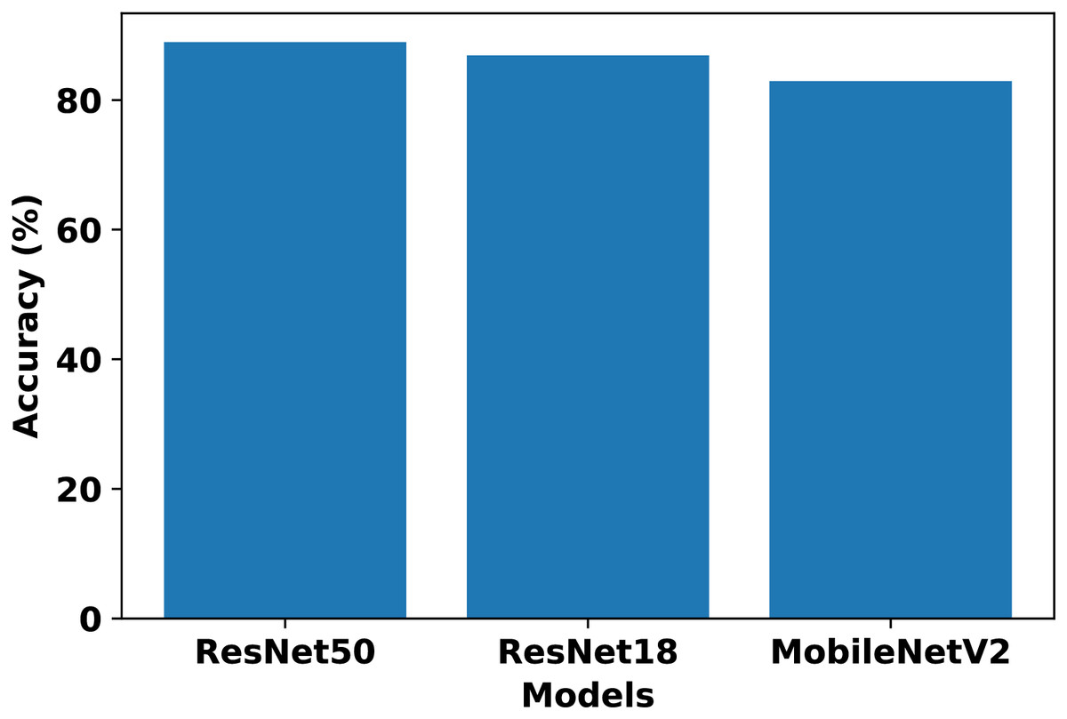
Figure 2: Comparison of ResNet50, ResNet18, and MobileNetV2 performance in the FL setup using FedAvg.
The differences in performance across the evaluated architectures can be explained by their design characteristics and adaptability to FL. ResNet50 achieved the best results due to its residual connections and sufficient depth, which improve gradient flow and stability during optimization, allowing the model to generalize effectively across heterogeneous client datasets. ResNet18 and MobileNetV2 performed competitively but have lower representational capacity compared to ResNet50, which limited their ability to extract more complex features in this setup. VGG19, despite its depth, lacks residual connections and contains a large number of parameters, making it prone to gradient vanishing and overfitting on clients with limited non-IID data. EfficientNet-B0 also underperformed, as its compound scaling strategy and reliance on stable batch normalization make it more sensitive to small batch sizes and heterogeneous client distributions. Overall, ResNet50 provided the best balance between depth, optimization stability, and generalization ability, making it the most suitable model for our FL setup.
Data augmentation
Before training, all images in the dataset underwent several pre-processing steps. To ensure uniformity, each image is resized to a consistent input dimension of pixels to match the input requirements of the ResNet50 architecture. The pixel values of the images are then normalized to a range of .
A significant challenge in our non-IID federated setup is the severe class imbalance present in each client’s local dataset. To address this, we employed data augmentation with two primary goals: to increase the diversity of the training data for better model generalization and to implement a targeted oversampling strategy (Khan et al., 2022c). To preserve the diagnostic integrity of medical images, augmentation parameters are carefully constrained to moderate ranges, selected based on previous studies (Mumuni & Mumuni, 2022; Khan et al., 2022b), ensuring that the augmented images remain clinically realistic while improving class balance. The following geometric augmentation techniques are applied, with any new pixels generated by the transformations filled using the nearest value (fill_mode="nearest"):
Shear range:
Zoom range:
Rotation range:
Width and height shift range:
Channel shift range:
Horizontal and vertical flips: Applied randomly.
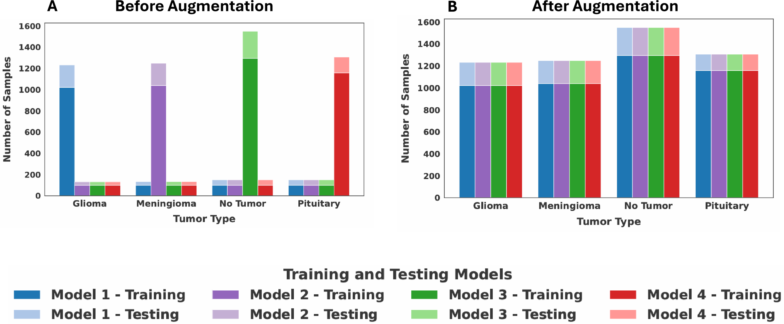
The goal of our augmentation strategy is to standardize the number of samples for each class across all clients, ensuring that each class contributes an equal amount of data to the overall FL process. This is implemented as follows: First, we identified the global maximum sample count for each of the four classes by examining the data distributions across all four clients, separately determining this maximum for both the training and testing sets. This count then served as the target number for that class. For each client, if a class contained fewer images than the target number, the augmentation techniques are applied exclusively to that class to generate augmented images until its sample count matches the target. Classes that already contain the maximum number of samples are not augmented. To provide a concrete example, Client 1 contained the maximum number of glioma training images (1,021 samples). Consequently, the glioma training sets for Clients 2, 3, and 4 are oversampled to also contain 1,021 images. This same process is repeated for all classes across both training and testing sets. The resulting balanced class distribution for all four clients after this standardization process is presented in Table 5. The dataset distribution among the four clients before and after data augmentation is shown in Fig. 3. Following augmentation, each client is a balanced set of all tumor classes to simulate IID data. This intentional realignment led to identical class distributions across clients. As a result, the JS Divergence between any pair of clients becomes zero, confirming the removal of heterogeneity among the clients.
| Class | Client 1 | Client 2 | Client 3 | Client 4 |
|---|---|---|---|---|
| Glioma | (1021, 210) | (1021, 210) | (1021, 210) | (1021, 210) |
| Meningioma | (1039, 210) | (1039, 210) | (1039, 210) | (1039, 210) |
| No tumor | (1295, 255) | (1295, 255) | (1295, 255) | (1295, 255) |
| Pituitary | (1157, 150) | (1157, 150) | (1157, 150) | (1157, 150) |
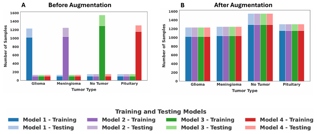
Figure 3: Dataset distribution among the four clients: (A) before augmentation, (B) after augmentation.
Proposed model architecture
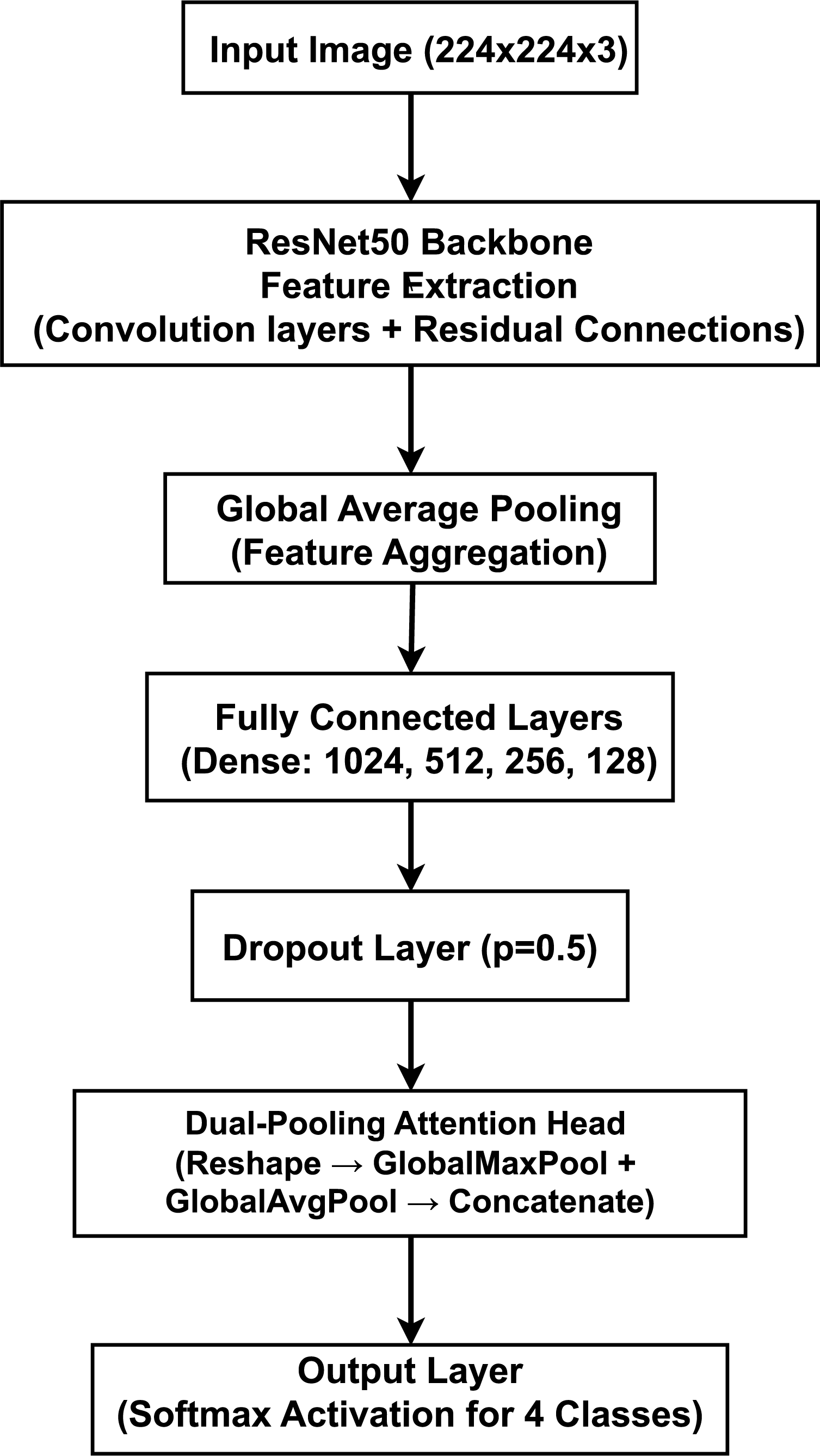
Our proposed model, illustrated in Fig. 4, is a deep CNN that employs a transfer learning strategy for multi-class brain tumor classification. The architecture is composed of three primary stages: (1) a pre-trained ResNet50 backbone for robust feature extraction, (2) a custom Multi-Layer Perceptron (MLP) head for classification, and (3) a novel dual-pooling Attention Head designed to refine the feature representation before the final prediction.
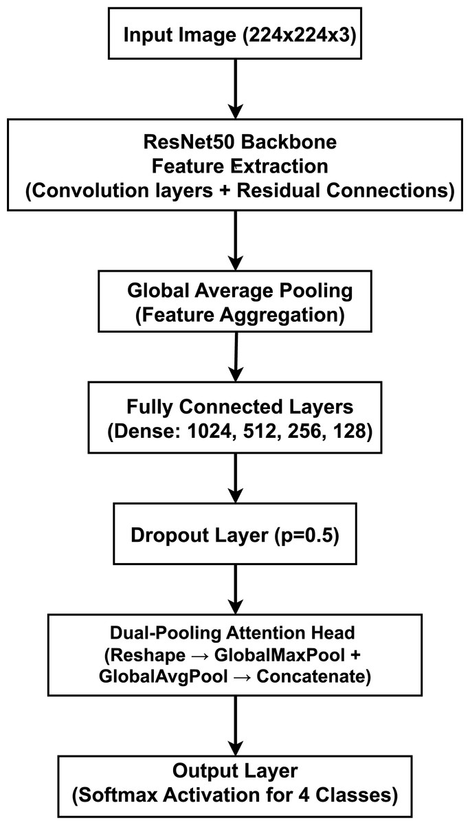
Figure 4: Proposed model architecture integrating a ResNet50 backbone with a dual-pooling attention head for brain tumor classification, illustrating the feature extraction and attention-based classification components.
The model is designed to process 2D slices of brain MRI scans, which are resized to an input dimension of . The final output is a four-element probability vector generated by a Softmax activation function, corresponding to the four target classes. The data propagates through the network sequentially. The input image is first processed by the ResNet50 model, pre-trained on the ImageNet dataset. We utilize the model as a powerful feature extractor by removing its original top classification layer (by setting include_top=False). The feature maps from the ResNet50 backbone are aggregated by a GlobalAveragePooling2D layer, which produces a single, flattened feature vector. The feature vector is then passed through a sequence of four fully connected (Dense) layers with 1,024, 512, 256, and 128 neurons, respectively. Each of these layers uses the Rectified Linear Unit (ReLU) activation function to introduce non-linearity. For regularization and to mitigate overfitting, a Dropout layer with a rate of is also applied. The resulting 128-dimensional feature vector is processed by our custom Attention Head. It is first reshaped into a 4D tensor of shape to be compatible with 2D pooling layers. This tensor is then processed in parallel by GlobalMaxPooling2D and GlobalAveragePooling2D operations. The outputs are combined using a Concatenate layer, resulting in a richer 256-dimensional feature vector. In the output layer, this final 256-dimensional vector is fed into a Dense layer with four neurons and a Softmax activation function to produce the final probability distribution over the classes.
The core novelty of our architecture lies in the dual-pooling attention head. By processing the feature vector through parallel max and average pooling streams, the head captures two complementary aspects of the learned features: the peak feature activations (using max pooling) and the overall feature context (using average pooling). Concatenating these two distinct representations provides the final classification layer with a more comprehensive feature set, enhancing the model’s ability to focus on both subtle, localized details and broader contextual patterns within the MRI scans.
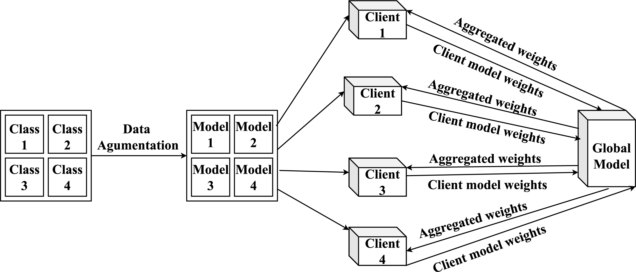
FedProx-based FL training
The FedProx implementation is presented in Algorithm 1 and the proposed FL architecture is outlined in Fig. 5. The FL process is conducted for a total of 100 communication rounds. In each round, participating clients trained their local models for one epoch on their respective datasets. The global model’s performance is evaluated, and the model state is saved after every 10-round segment. To avoid overfitting and unnecessary computation, we employed an early stopping mechanism with a patience of 20 rounds, which monitored the validation loss. The model with the best-performing validation loss is preserved at the end of each segment. The core hyperparameters for our experiments are summarized in Table 6.
| 1: Input: Number of clients K, number of rounds , regularization parameter μ, local epochs E, global model |
| 2: for each round to do |
| 3: for each client to K in parallel do |
| 4: Initialize local model |
| 5: for each epoch to E do |
| 6: Compute gradient: |
| 7: Update local model: |
| 8: end for |
| 9: end for |
| 10: Aggregate models: |
| 11: end for |
| 12: Output: Global model |
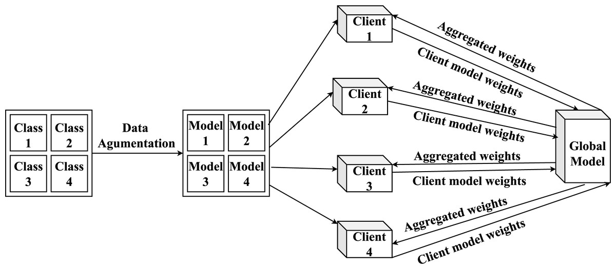
Figure 5: Overview of the proposed FL model architecture and its workflow.
| Parameter | Value |
|---|---|
| FL algorithm | FedProx |
| FL communication rounds | 100 |
| Local training epochs | 1 |
| Optimizer | SGD (Stochastic gradient descent) |
| Loss function | Sparse categorical cross-entropy |
| Learning rate | |
| Early stopping patience | 20 rounds |
| Batch size | 32 |
The values for the FedProx proximal regularization parameter, , are deliberately chosen to systematically probe the effect of the regularization strength on model performance in our highly non-IID environment. As controls the contribution of the proximal term , it serves as a hyperparameter that requires tuning for different datasets and levels of data heterogeneity. The selection process of is structured as follows:
Baseline comparison: The value is selected as a critical baseline, as this configuration makes the FedProx algorithm mathematically equivalent to the standard FedAvg algorithm.
Spectrum of regularization: The values (weak), and (intermediate), and (strong) are chosen as representative points to map out the impact of increasing regularization strength on client drift and model convergence. In this context, a smaller value makes the penalty for drifting weaker, which is why it is considered weak regularization, while a larger value imposes a stronger constraint.
This manual selection gave us a clear view of the trade-off between local model adaptation and global convergence, while avoiding the high computational cost of an exhaustive hyperparameter search in FL.
All experiments are carried out using an NVIDIA DGX server (RTX 3060 GPU) on an Acer laptop with Windows 11 OS, 16 GB of RAM, and Jupyter Notebook, along with PyTorch and TensorFlow libraries.
Results
To assess the performance of the proposed model, a hold-out validation strategy is employed. A separate test set is used to evaluate the performance of the global model. This held-out test set remains constant and is not subjected to resampling or k-fold partitioning. In this way, it distinguishes our approach from cross-validation-based evaluation. Performance is evaluated using key classification metrics such as accuracy, precision, recall, F1-score, and loss (Thiriveedhi et al., 2025).
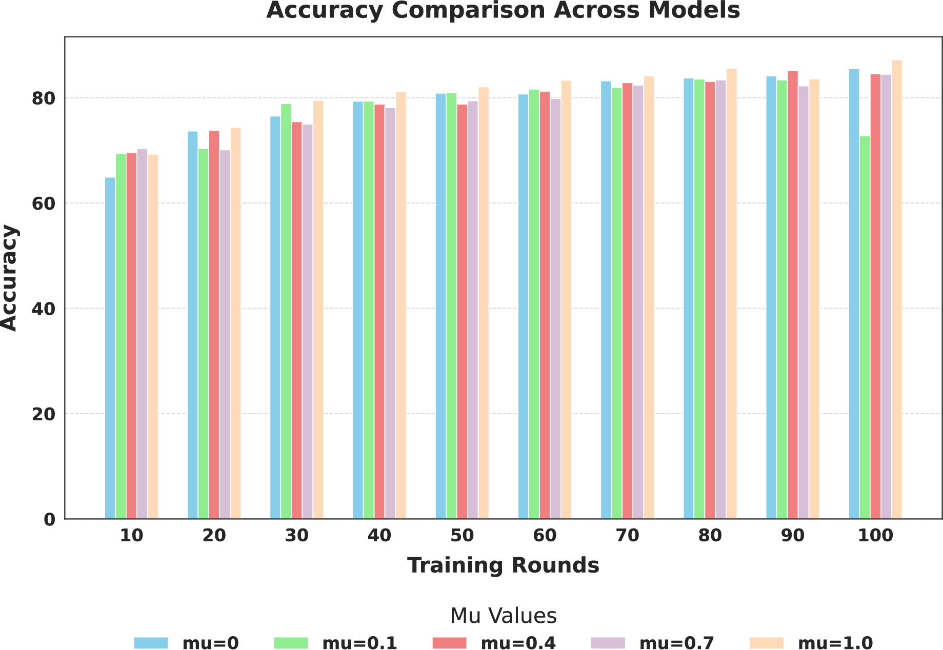
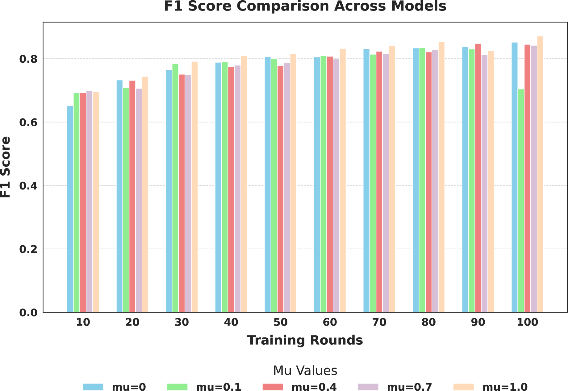
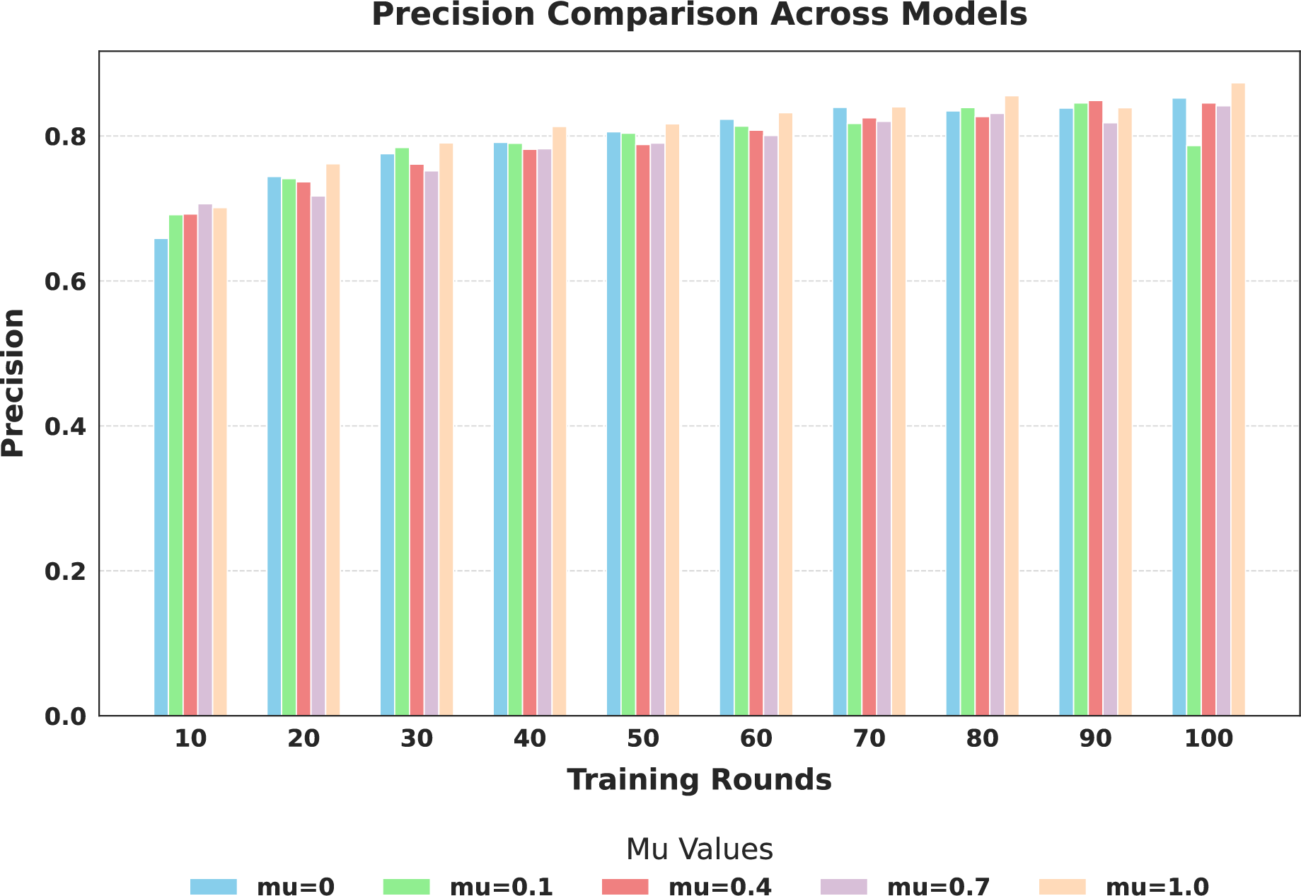
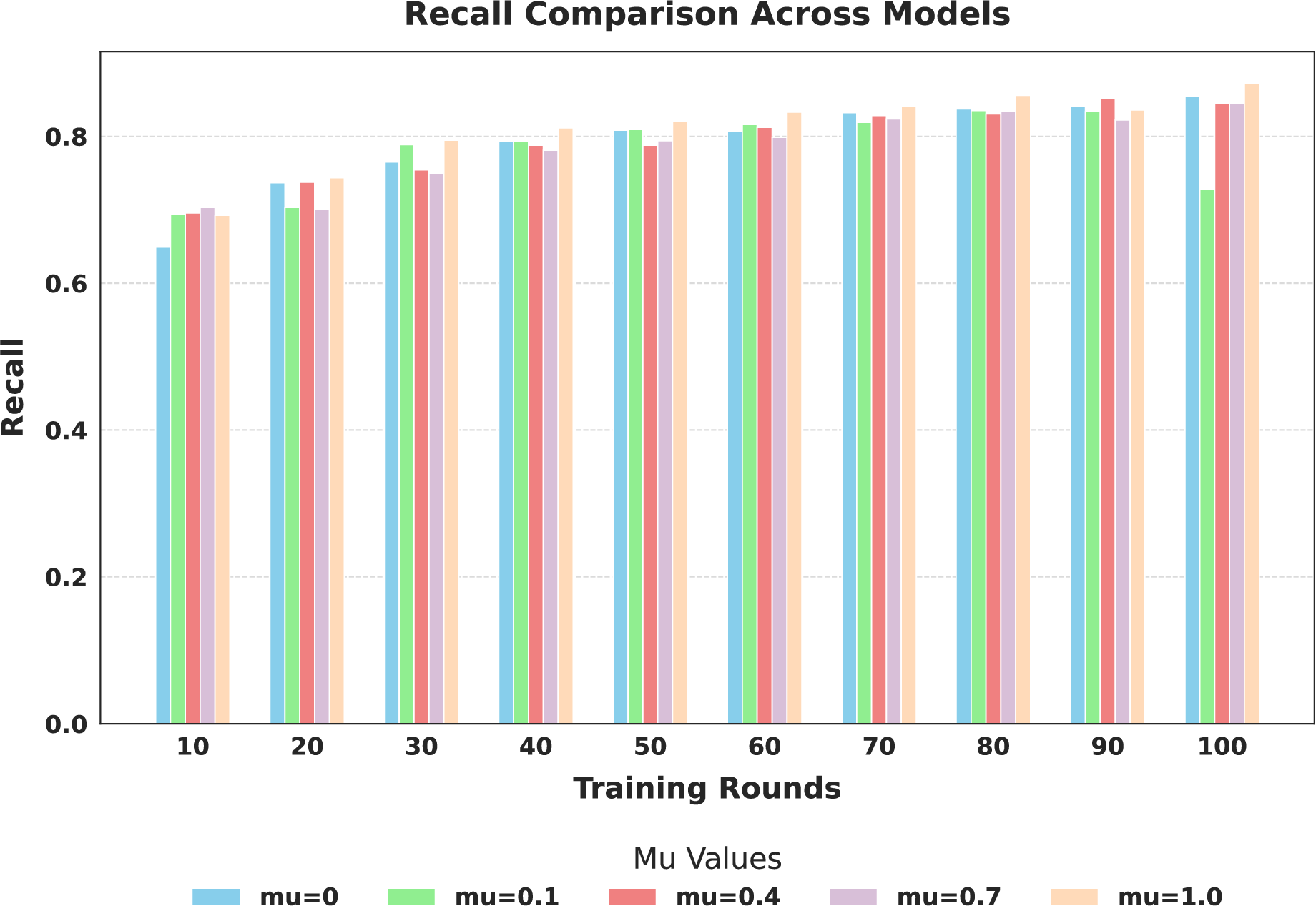
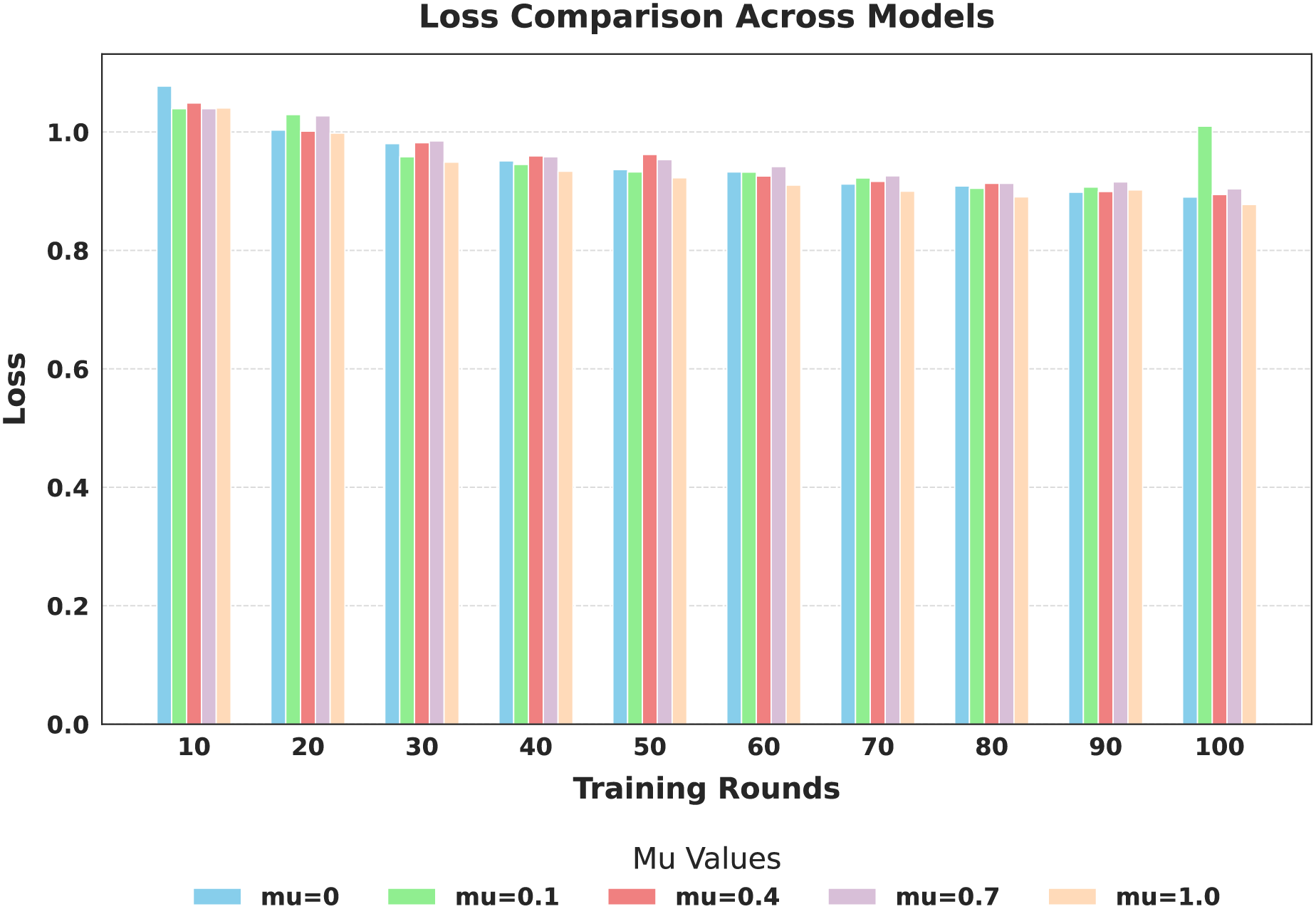
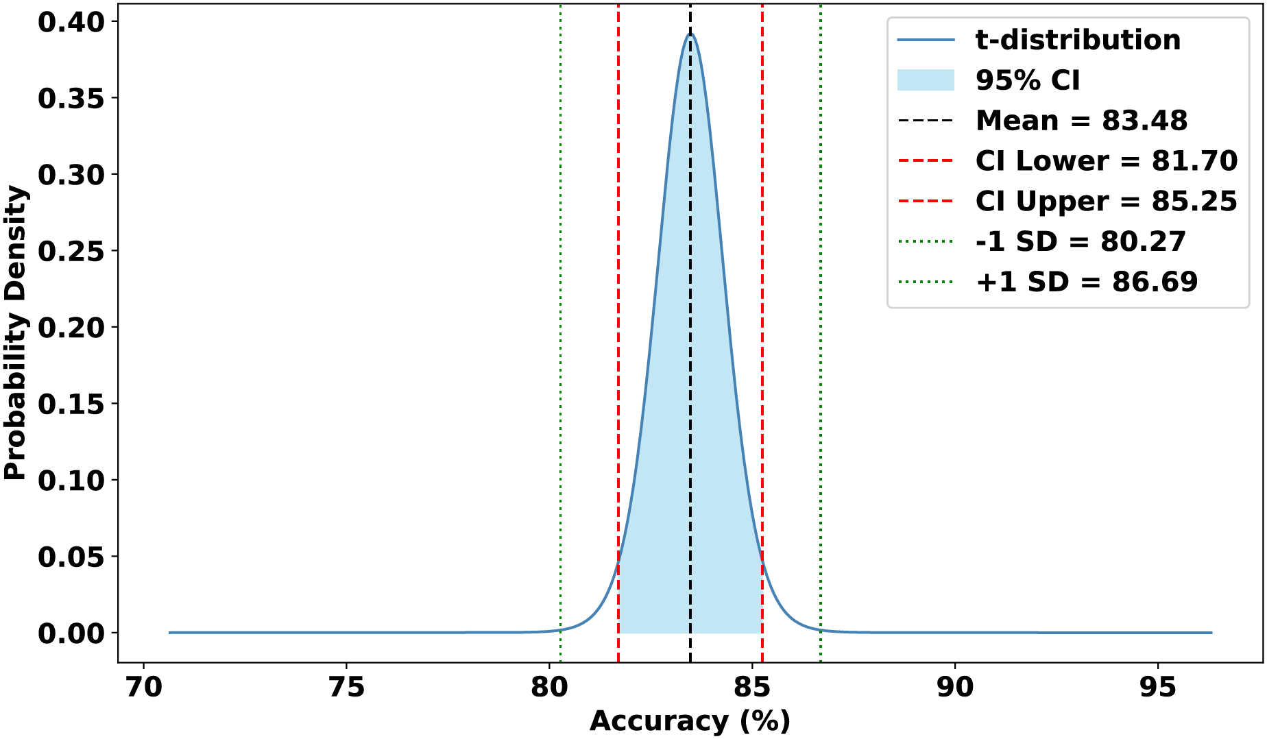
The evaluation focused on the global model’s performance trained over 100 communication rounds under various settings of the FedProx regularization term . Tables 7 and 8, along with Figs. 6–10, provide a comprehensive overview of how different values influenced the model’s performance over 100 rounds. Among all configurations, consistently outperformed other values across nearly all metrics, achieving the highest accuracy (87.19%), lowest loss, and superior precision, recall, and F1-score. This result confirms that strikes the best balance between personalization and regularization, effectively addressing client drift and variability in non-IID data. To quantify variability, we conducted a statistical analysis, and the results are presented in Fig. 11. The standard deviation of 3.2070 and the relatively narrow 95% confidence interval ([81.70–85.25]) for the global model’s classification accuracy indicate that the results are consistent across rounds, suggesting stable performance of the proposed method. FedAvg ( ) provided decent baseline results, but is outperformed by , indicating that the regularization avoids overfitting to local distributions and provides enhanced generalization in the global model. A paired t-test is performed to statistically validate the observed performance differences between FedAvg and the proposed FedProx approach,. The test yielded a significant result ( , ). The value of less than 0.05 confirms that the improvement achieved by FedProx over FedAvg is statistically significant.
| Metric | Round 10 | Round 20 | Round 30 | Round 40 | Round 50 | Round 60 | Round 70 | Round 80 | Round 90 | Round 100 | |
|---|---|---|---|---|---|---|---|---|---|---|---|
| 0.0 | Accuracy | 64.91 | 73.68 | 76.51 | 79.33 | 80.85 | 80.70 | 83.22 | 83.75 | 84.13 | 85.51 |
| Precision | 0.6586 | 0.7439 | 0.7754 | 0.7911 | 0.8057 | 0.8231 | 0.8395 | 0.8345 | 0.8385 | 0.8523 | |
| F1-score | 0.6518 | 0.7325 | 0.7656 | 0.7886 | 0.8064 | 0.8052 | 0.8312 | 0.8336 | 0.8377 | 0.8518 | |
| Recall | 0.6491 | 0.7368 | 0.7651 | 0.7933 | 0.8085 | 0.8070 | 0.8322 | 0.8375 | 0.8413 | 0.8551 | |
| Loss | 1.0776 | 1.0031 | 0.9802 | 0.9512 | 0.9365 | 0.9324 | 0.9121 | 0.9087 | 0.8982 | 0.8901 | |
| 0.1 | Accuracy | 69.41 | 70.33 | 78.87 | 79.33 | 80.93 | 81.62 | 81.92 | 83.52 | 83.37 | 72.77 |
| Precision | 0.6913 | 0.7410 | 0.7841 | 0.7899 | 0.8038 | 0.8135 | 0.8173 | 0.8391 | 0.8456 | 0.7866 | |
| F1-score | 0.6922 | 0.7094 | 0.7840 | 0.7902 | 0.8008 | 0.8091 | 0.8139 | 0.8342 | 0.8301 | 0.7043 | |
| Recall | 0.6941 | 0.7033 | 0.7887 | 0.7933 | 0.8093 | 0.8162 | 0.8192 | 0.8352 | 0.8337 | 0.7277 | |
| Loss | 1.0394 | 1.0294 | 0.9582 | 0.9451 | 0.9325 | 0.9321 | 0.9223 | 0.9049 | 0.9071 | 1.0097 | |
| 0.4 | Accuracy | 69.57 | 73.76 | 75.44 | 78.79 | 78.79 | 81.24 | 82.84 | 83.07 | 85.13 | 84.52 |
| Precision | 0.6924 | 0.7368 | 0.7612 | 0.7815 | 0.7882 | 0.8079 | 0.8251 | 0.8268 | 0.8488 | 0.8454 | |
| F1-score | 0.6927 | 0.7315 | 0.7509 | 0.7748 | 0.7787 | 0.8074 | 0.8231 | 0.8212 | 0.8480 | 0.8451 | |
| Recall | 0.6957 | 0.7376 | 0.7544 | 0.7879 | 0.7879 | 0.8124 | 0.8284 | 0.8307 | 0.8513 | 0.8452 | |
| Loss | 1.0490 | 1.0014 | 0.9819 | 0.9595 | 0.9621 | 0.9256 | 0.9166 | 0.9132 | 0.8993 | 0.8944 | |
| 0.7 | Accuracy | 70.33 | 70.10 | 74.98 | 78.11 | 79.41 | 79.86 | 82.38 | 83.37 | 82.23 | 84.44 |
| Precision | 0.7064 | 0.7172 | 0.7519 | 0.7823 | 0.7901 | 0.8006 | 0.8202 | 0.8311 | 0.8182 | 0.8415 | |
| F1-score | 0.6981 | 0.7064 | 0.7488 | 0.7793 | 0.7880 | 0.7988 | 0.8158 | 0.8274 | 0.8116 | 0.8420 | |
| Recall | 0.7033 | 0.7010 | 0.7498 | 0.7811 | 0.7941 | 0.7986 | 0.8238 | 0.8337 | 0.8223 | 0.8444 | |
| Loss | 1.0394 | 1.0272 | 0.9849 | 0.9580 | 0.9532 | 0.9414 | 0.9259 | 0.9132 | 0.9157 | 0.9039 | |
| 1.0 | Accuracy | 69.26 | 74.37 | 79.48 | 81.16 | 82.07 | 83.30 | 84.13 | 85.58 | 83.60 | 87.19 |
| Precision | 0.7011 | 0.7615 | 0.7903 | 0.8130 | 0.8167 | 0.8321 | 0.8402 | 0.8554 | 0.8390 | 0.8734 | |
| F1-score | 0.6950 | 0.7441 | 0.7916 | 0.8098 | 0.8154 | 0.8323 | 0.8398 | 0.8543 | 0.8255 | 0.8716 | |
| Recall | 0.6926 | 0.7437 | 0.7948 | 0.8116 | 0.8207 | 0.8330 | 0.8413 | 0.8558 | 0.8360 | 0.8719 | |
| Loss | 1.0405 | 0.9980 | 0.9492 | 0.9336 | 0.9227 | 0.9102 | 0.8999 | 0.8904 | 0.9020 | 0.8774 |
| Precision (%) | Recall (%) | F1-score (%) | |
|---|---|---|---|
| Glioma | 89.02 | 78.33 | 83.33 |
| Meningioma | 75.38 | 80.07 | 77.65 |
| No tumor | 92.60 | 95.80 | 94.17 |
| Pituitary | 90.76 | 91.67 | 91.21 |
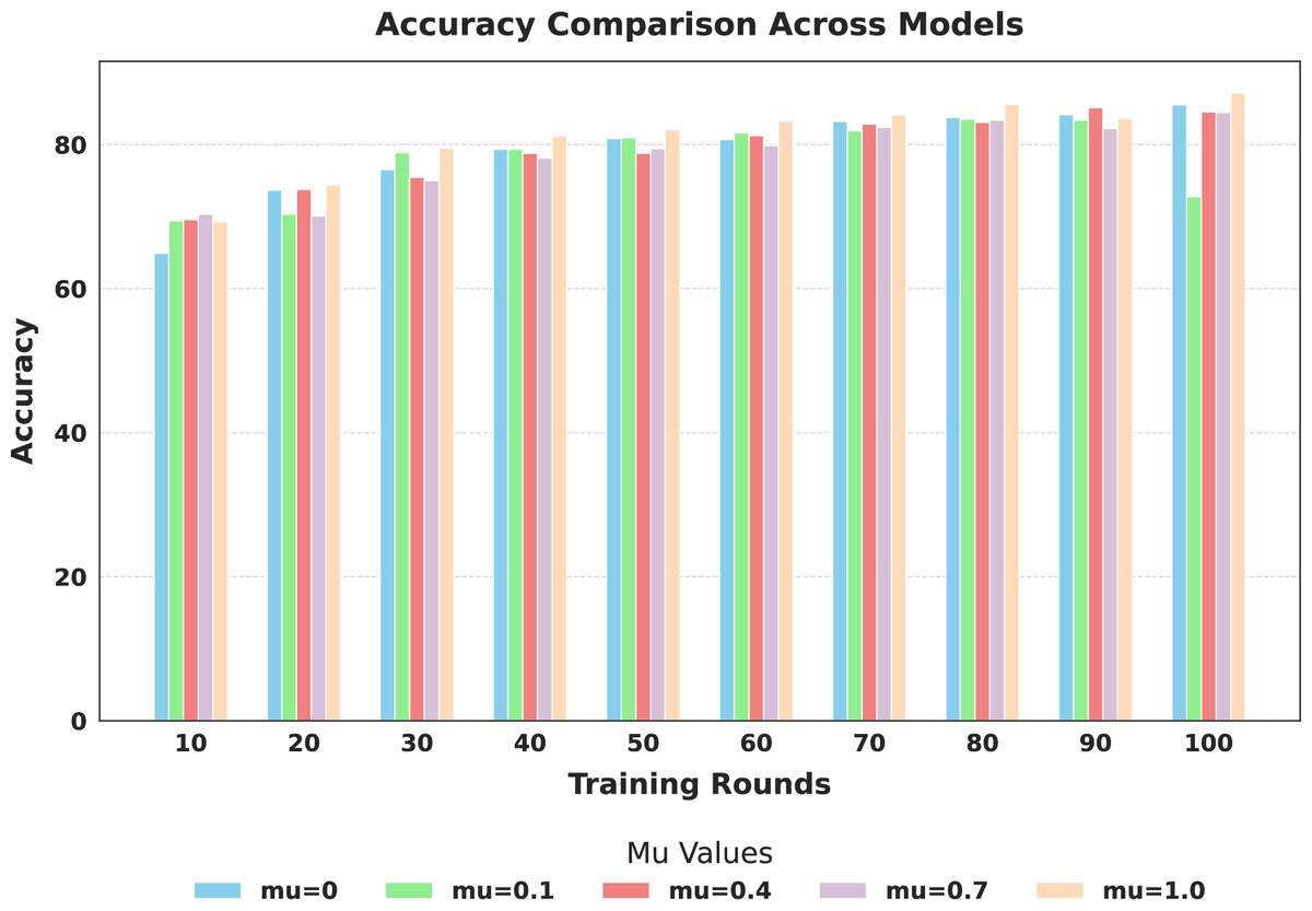
Figure 6: Comparison of global model accuracy across training rounds under different mu values.

Figure 7: Comparison of global model F1-score across training rounds under different mu values.

Figure 8: Comparison of global model precision across training rounds under different mu values.
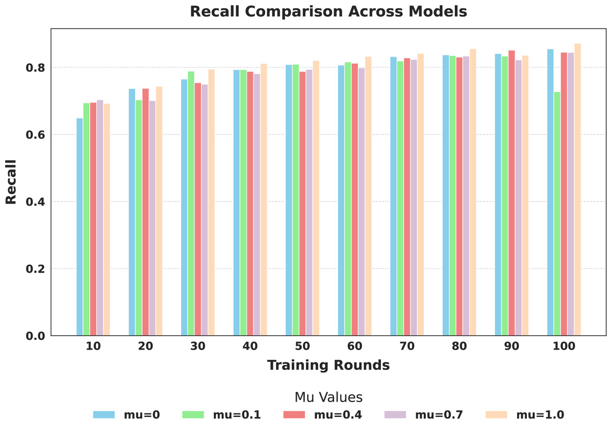
Figure 9: Comparison of global model recall across training rounds under different mu values.
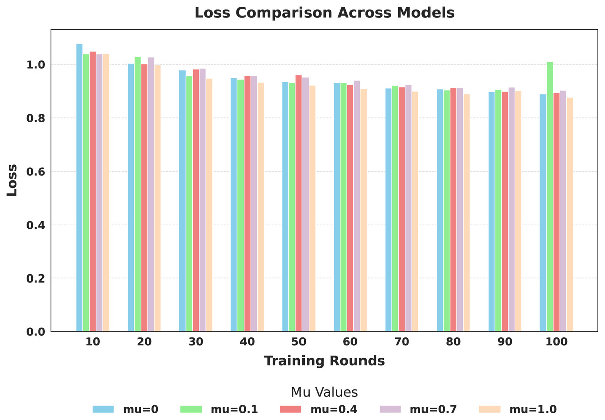
Figure 10: Comparison of global model loss across training rounds under different mu values.
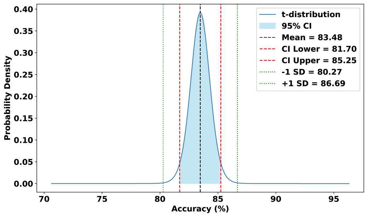
Figure 11: Statistical analysis of the proposed approach.
Importantly, the observed accuracy of 87.18% under extreme non-IID settings is a direct consequence of significant divergence in client data distributions, which is quantitatively supported by the JS divergence values computed across clients. The high JS divergence reflects substantial statistical differences in class distributions and feature spaces among client datasets, leading to model inconsistency and learning instability. This heterogeneity introduces conflicting gradient updates during aggregation, thereby making global convergence more challenging and reducing the overall classification performance.
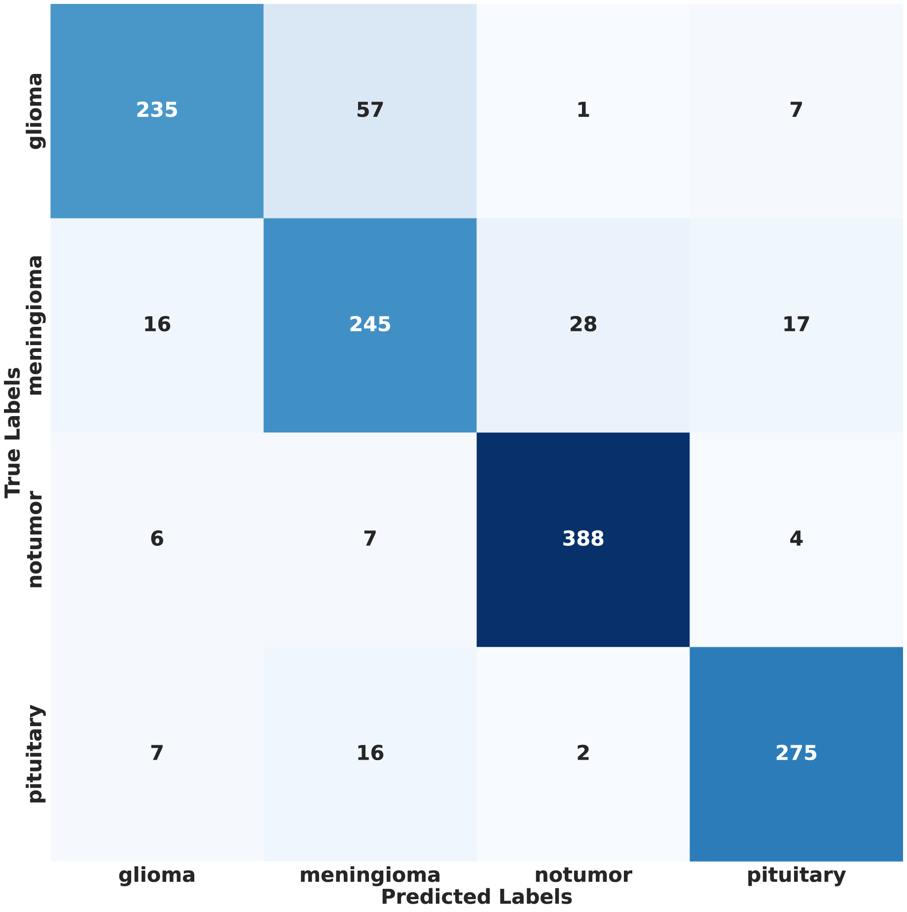
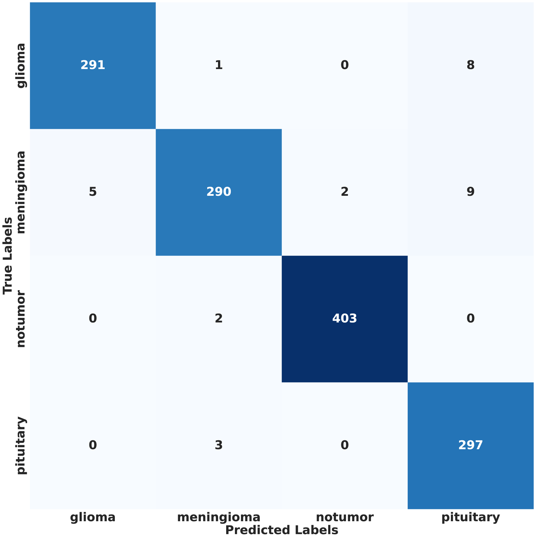
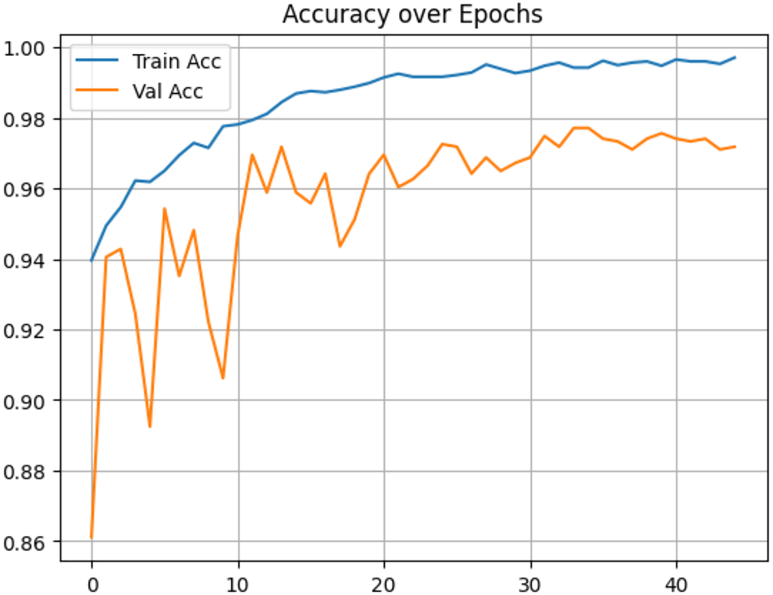
In contrast, under IID conditions, the proposed model achieved a final accuracy of 97.71% and a minimal test loss of 0.0628. The confusion matrices in Figs. 12 and 13 further highlight classification strengths and weaknesses across tumor categories. Experiments with direct IID data demonstrated markedly better convergence behavior and generalization performance, as shown in Fig. 14. The substantial performance gap between IID and non-IID scenarios underscores the strong influence of client data heterogeneity on FL outcomes. To the best of our knowledge, no previous study has evaluated FL performance across such extreme-divergence client datasets while achieving this level of classification accuracy. These results establish a new baseline for divergence-aware FL in medical imaging and demonstrate that careful tuning of the FedProx regularization parameter can substantially mitigate the negative effects of statistical heterogeneity, even under challenging real-world data conditions.
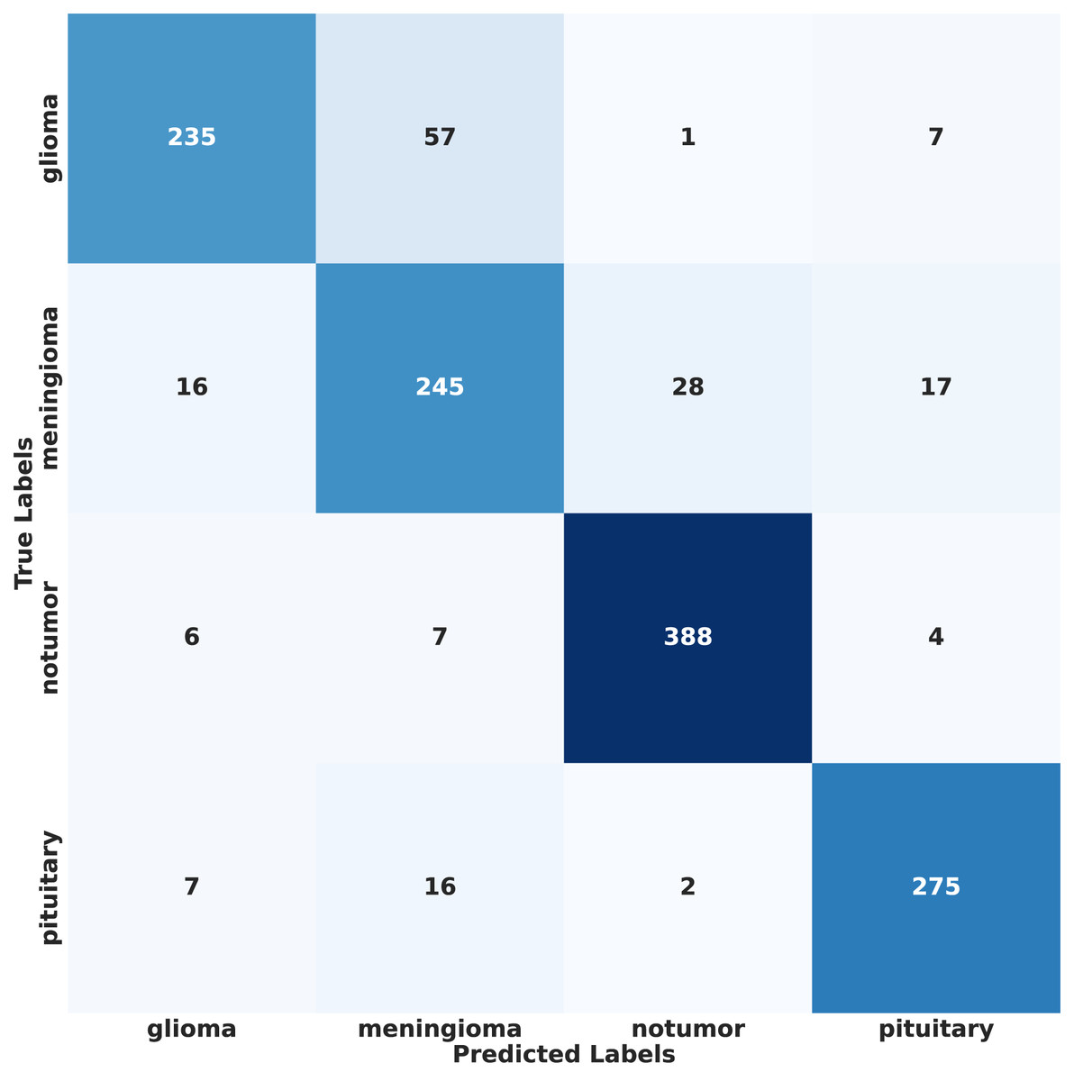
Figure 12: Confusion matrix of proposed model on non-IID data.
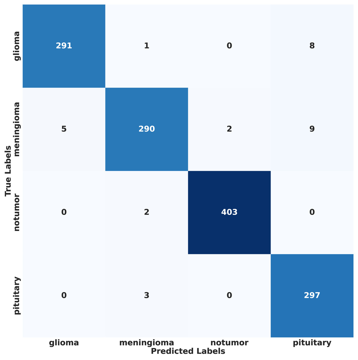
Figure 13: Confusion matrix of proposed model results on IID data.
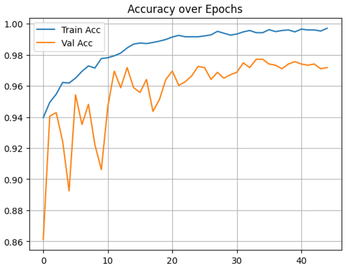
Figure 14: Accuracy of proposed model on IID data.
Discussion
Without FL
The results of our proposed model, which utilized FL with non-IID data, demonstrate its ability to handle decentralized and heterogeneous data while maintaining competitive performance. This stands in contrast to prior works that relied on models trained with IID data and centralized learning. For instance, Vidyarthi et al. (2022) achieved an accuracy of 95.86% using a neural network classifier with a cumulative variance feature extraction method on the Kaggle dataset; similarly, Khan et al. (2022a) developed a hierarchical DL model (HDL2BT) with 92.13% accuracy. Other studies, such as Senan et al. (2022) and Nazir et al. (2024), explored AlexNet-SVM and explainable AI approaches, obtained 94.64% and 95.10% accuracy, respectively. While these studies reported good performance, their reliance on IID data and centralized learning limits their applicability to real-world decentralized scenarios. In contrast, our FL approach addresses these challenges by enabling collaboration across distributed clients with non-IID data, achieving comparable results despite the complexities of the FL paradigm. This highlights the robustness and practicality of FL in handling real-world data distributions while maintaining strong model performance. The comparison of existing works without using FL is summarized in Table 9.
| Reference | Approach | Accuracy (%) |
|---|---|---|
| Khan et al. (2022a) | Hierarchical DL based BTC (HDL2BT) | 92.13 |
| Vidyarthi et al. (2022) | NN Classifier with cumulative variance method for feature extraction | 95.86 |
| Nazir et al. (2024) | CNN along with explainable AI | 94.64 |
| Senan et al. (2022) | AlexNet-SVM | 95.10 |
With FL and using IID and non-IID data
Compared to existing literature, our proposed model demonstrates a robust solution. Specifically, it employs the ResNet50 attention model in an FL setting with IID data, and when extended with data augmentation and the FedProx algorithm in a non-IID setting, it effectively handles decentralized, heterogeneous data distributions. Previous works, such as Ay, Ekinci & Garip, 2024, utilized the FedAvg algorithm and achieved an accuracy of 85.55%, using FL with IID data. Similarly, Talukder, Islam & Uddin, 2023 achieved 91.05% accuracy using a voting ensemble of six transfer learning models with FL on the Kaggle dataset, also assuming IID data distributions. Zhou, Wang & Zhou, 2024 explored FL with EfficientNetB0 and ResNet50 on the SARTAJ dataset, achieved accuracy rates of 80.17% and 65.32%, respectively, again under IID assumptions. Table 10 presents a comparison of the results of the existing and proposed works. As expected, the model performed better in an ideal and perfectly balanced IID setting. This is because our realistic non-IID setup causes “client drift”, where each client’s biased data pulls the shared global model in conflicting directions, making it harder to learn. While our oversampling strategy helped counter this, it came with a trade-off. Augmenting images adds quantity but doesn’t introduce new, unique patient cases or biological patterns. This lack of true diversity in the original data helps explain the performance ceiling we observed (87.19% accuracy), highlighting the challenge of training with real-world, heterogeneous data.
| Reference | Approach | Accuracy (%) |
|---|---|---|
| Talukder, Islam & Uddin (2023) | Ensemble DL model using grid search-based weight optimization (GSWO) | 91.05 |
| Zhou, Wang & Zhou (2024) | ResNet50 and EfficientNetB0 | 65.32 |
| 80.17 | ||
| Ay, Ekinci & Garip (2024) | FedAvg | 85.55 |
| Ft-FedAvg | 85.8 | |
| Proposed work | ResNet50-Attention model (IID) | 97.71 |
| ResNet50-Attention model + DA+ FedProx (non-IID) | 87.19 |
Although Muntaqim & Smrity (2025) reported a higher accuracy of 98.24%, claiming to have considered non-IID data, the actual heterogeneity in their setup was very low. To more precisely quantify the heterogeneity in our dataset, we computed the Jensen–Shannon Divergence (JSD) between clients. Table 11 presents the JSD matrix from the aforementioned study (Muntaqim & Smrity, 2025) and our proposed work. In Muntaqim & Smrity (2025), the client distributions were considerably more homogeneous, as reflected by significantly lower divergence values; the highest divergence reported is 0.0258, whereas our setup reaches a maximum divergence of 0.533, an extremely high value, highlighting the substantial heterogeneity in our case. This pronounced heterogeneity, particularly the extreme class imbalance across clients, is the primary reason for the relatively lower performance of our model. Such an imbalance significantly impacts the global model’s ability to generalize. Nevertheless, despite these challenges, our approach demonstrated promising results under more realistic and complex data conditions.
| Work | Client | C1 | C2 | C3 | C4 |
|---|---|---|---|---|---|
| Existing work (Muntaqim & Smrity, 2025) | C1 | 0.0000 | 0.0160 | 0.0206 | 0.0232 |
| C2 | 0.0160 | 0.0000 | 0.0258 | 0.0333 | |
| C3 | 0.0206 | 0.0258 | 0.0000 | 0.0203 | |
| C4 | 0.0232 | 0.0333 | 0.0203 | 0.0000 | |
| Proposed work (Ours) | C1 | 0.0000 | 0.483 | 0.515 | 0.499 |
| C2 | 0.483 | 0.0000 | 0.518 | 0.501 | |
| C3 | 0.515 | 0.518 | 0.0000 | 0.533 | |
| C4 | 0.499 | 0.501 | 0.533 | 0.0000 |
Conclusion
This study successfully demonstrated the application of FL for BTC using a non-IID dataset, addressing the critical challenge of data heterogeneity. The use of the FedProx algorithm, with its proximal regularization term ( ), proved an effective method in mitigating clients’ divergence and enhancing model stability in non-IID settings. Data augmentation also played a crucial role in ensuring uniform performance across all clients, enabling fair and effective FL. We considered a range of values for the FedProx proximal regularization term ( and ) and tuned them in our experimental setting. Among these, outperformed the others, achieving a global model accuracy of 87.19% and an F1-score of 87.16%. This indicates the significance of proximal regularization in achieving robust model convergence. Even when the loss values remained around 0.8 for both FedAvg and , the superior performance with underscores the importance of regularization in enhancing stability and performance in non-IID federated scenarios. The primary motivation of this work is to investigate the feasibility and impact of implementing the FedProx algorithm in highly non-IID environments, where client data divergence poses major challenges to convergence and accuracy. Due to the complexity of training with non-IID data in terms of computational resources and time, transfer learning is adopted to ensure manageable training cycles while retaining sufficient capacity for meaningful classification. The framework achieved compelling results, establishing a practical baseline for future work in federated medical imaging. The practical implications of this work are significant, offering a path to democratize diagnostic expertise for smaller clinics and improve consistency by serving as a decision support tool for radiologists.
Future work
While this study demonstrates the efficacy of FedProx in addressing non-IID data challenges, it also highlights areas for further exploration. Future work may explore different combinations of augmentation techniques to better understand their specific contributions to mitigating non-IID bias in FL. The achieved accuracy, while promising, suggests scope for improvement in optimizing model performance. Looking ahead, future work to bridge the performance gap in non-IID settings could focus on exploring Personalized FL (PFL) to create client-specific models. The geometric augmentation (e.g., rotation, flipping, scaling) only slightly alters existing images; they cannot create entirely new, realistic variations, which may limit model generalization. Employing advanced data synthesis, such as Generative Adversarial Networks (GAN), overcomes the limitations of geometric augmentation. Developing adaptive algorithms to dynamically tune the regularization parameter ( ) could allow the model to automatically explore optimal values, potentially improving performance and reducing the need for manual parameter selection. Future research could explore incorporating blockchain technology to establish a secure and transparent framework for managing model updates and participant contributions, thereby enhancing trust and traceability in decentralized settings. Incentive mechanisms, potentially built on blockchain-based smart contracts, could further encourage sustained and honest participation from diverse clients. We would like to extend our work to other medical image analysis tasks. Expanding the study to larger, more diverse datasets and evaluating real-world deployment scenarios would also help validate the scalability and robustness of the approach, potentially paving the way for secure, privacy-preserving AI applications in healthcare.