
Multi-level functional network-based PD identification via graph deep learning
- Published
- Accepted
- Received
- Academic Editor
- Giovanni Angiulli
- Subject Areas
- Algorithms and Analysis of Algorithms, Artificial Intelligence, Data Mining and Machine Learning, Optimization Theory and Computation, Neural Networks
- Keywords
- Parkinson’s disease, fMRI, GCN, Laplacian regularization, Frontal lobe
- Copyright
- © 2026 Lu and Zhao
- Licence
- This is an open access article distributed under the terms of the Creative Commons Attribution License, which permits unrestricted use, distribution, reproduction and adaptation in any medium and for any purpose provided that it is properly attributed. For attribution, the original author(s), title, publication source (PeerJ Computer Science) and either DOI or URL of the article must be cited.
- Cite this article
- 2026. Multi-level functional network-based PD identification via graph deep learning. PeerJ Computer Science 12:e3392 https://doi.org/10.7717/peerj-cs.3392
Abstract
Background
Parkinson’s disease (PD) is a neurodegenerative disease characterized by degenerative changes in nigrostriatal dopaminergic neurons and Lewy body morphology. Functional magnetic resonance imaging (fMRI) has become an important tool for identifying biomarkers of PD by virtue of its sensitivity in detecting differences in functional connectivity (FC) of the brain. Most of the current FC-based PD diagnostic methods only consider the connectivity topology between brain regions, ignoring the differences and complementarities of FCs between patients, which have been proven to be critical in identifying PD.
Methods
In this article, a patient similarity network is first constructed to mine the complementarity of FC between patients, and a multi-level functional network structure is constructed, which consists of FCs between brain regions as well as the patient similarity network. Then, a graph convolutional network (GCN) model is established to extract the complex structural information of the multi-level network. Meanwhile, to avoid the overfitting problem that may be caused by the small sample of fMRI, the Laplacian regularization term is enforced in the GCN model.
Results
The results of the study show that the multi-level functional network structure based classification model performs well in PD identification with high levels of accuracy, precision, and recall of 76.2%, 72.2% and 75.3%, respectively. In addition, the role of different brain networks in the categorization task was deeply analyzed by the occlusion sensitivity analysis method, and it was found that the frontal lobe has an important role in recognizing PD. The work verified the significance of complementarity of FC between patients in identifying PD.
Introduction
Parkinson’s disease (PD) is a common and complex movement disorder that usually occurs in the middle-aged and elderly population (Zhong et al., 2023), and is medically ranked as the second most common neurodegenerative disease in terms of prevalence (Arsland et al., 2021). At the pathological level, PD is a chronic neurological disorder that mainly affects nigrostriatal dopaminergic neurons in the brain, with resting tremor, increased dystonia, bradykinesia, and postural balance disorders constituting the typical clinical manifestations of the disease (Bu, Pang & Fan, 2023). The incidence and prevalence of Parkinson’s disease increases significantly with age. Accelerated global aging and the rapid growth of the elderly population have led to a continued increase in the number of patients with Parkinson’s disease (Ying Liu & Chan, 2016). Therefore, the early and accurate identification of PD is crucial for formulating effective treatment plans and improving the prognosis of patients (Guo, Tinaz & Dvornek, 2022). Liu (2021) achieved early intelligent diagnosis of PD by combining machine learning and gait signal analysis. Jin et al. (2020) made an important contribution to the early diagnosis of PD by monitoring metabolic changes in substantia nigra (SN) and globus pallidus (GP) in PD patients.
Magnetic resonance imaging (MRI) has developed into an important tool in neuroscience research (Zhu et al., 2024; Chen et al., 2019). In recent years, resting state functional magnetic resonance imaging (rs-fMRI) has shown unique advantages in the study of motor and non-motor symptoms, disease severity and neural mechanism of PD by detecting the blood oxygen level dependent (BOLD) signal (Qu et al., 2021; Tinaz, 2021). Chen et al.’s (2019) team made an important breakthrough in PD differential diagnosis by using this technology. By analyzing rs-fMRI data of PD patients, Lu (2023) not only revealed disease-related motor dysfunction features, but also established a diagnostic method based on functional connectivity. The key point is that the BOLD time series reflects the spontaneous neural activity of the brain. The statistical correlation performance of signals in different brain regions effectively characterizes the functional connection patterns of the brain, providing a new perspective for understanding the neural mechanism of PD (Kong et al., 2021; Greicius et al., 2003; Sunil et al., 2024).
Functional connectivity (FC) can reveal the interactions between brain regions during functional tasks, reflecting their coordinated activity (Chen & Yu, 2019). Resting-state brain functional connectivity analysis has become an important hotspot in neuroscience research in recent years, and it has far-reaching implications and important clinical significance in the diagnosis and mechanism understanding of certain brain diseases (Yang et al., 2015). Further, by analyzing the spatial topology of functional connectivity, the organizational features of brain networks and their functional configurations can be explored in depth, thus revealing the complex interactions of the brain in information processing (Di & Biswal, 2015; Yuan & Li, 2018). Shen (2023) focused on the changes in FC by analyzing rs-fMRI data from PD patients, which led to a deeper understanding of the pathophysiological mechanisms in patients. Wu et al. (2023) brought important implications for clinical research by studying FC changes between executive control networks and motor-related brain networks in PD patients. However, the above-mentioned studies mainly focused on the FC changes within individual patients, but generally ignored a key factor: the similarity of FC patterns among patients. This similarity feature contains commonality and difference information at the group level, which is crucial for accurately identifying disease biomarkers (Qu et al., 2021).
With the development of artificial intelligence technology, machine learning (ML) algorithms have shown great potential in the field of brain disease diagnosis, and several studies have explored the effectiveness of ML methods in early PD diagnosis by analyzing rs-fMRI data. For example, in Yang et al.’s (2023) study, they developed a 3D ResNet utilizing a convolutional neural network (CNN) which is capable of identifying PD from whole-brain MRI, and (Abós et al., 2017) by collecting rs-fMRI data from healthy individuals and patients with Parkinson’s disease, they reconstructed a functional connectivity map of the brain and applied a support vector machine (SVM) algorithm in machine learning to diagnose patients with Parkinson’s disease (Lu et al., 2023).
FC can be represented as a graph structure encoding interactions between brain regions. However, existing machine learning algorithms fail to fully exploit its complex network properties and overlook the complementary information from inter-subject FC variations. Inter-subject similarity features possess the capability to capture complex relationships among patients, identify potential differences between individuals, and exhibit strong robustness to noise and outliers. These features not only enhance diagnostic precision but also open new avenues for exploring brain functional networks. Recent studies by Qu et al. (2021). have demonstrated that similarity in patient FC patterns plays a pivotal role in neurological disorder identification, effectively pinpointing key brain networks and regions closely associated with cognitive functions. Nevertheless, current PD diagnostic models predominantly focus on intra-subject FC patterns, neglecting the potential of inter-subject relational features. This limitation arises from two critical challenges: (1) Conventional methods lack mechanisms to model population-level similarity among patients, which could reduce intra-class variability and improve feature discriminability; (2) The small sample size of fMRI data exacerbates overfitting risks when capturing high-dimensional FC features. To address these issues, we construct a multi-level functional network integrating individual FC networks with a subject-subject similarity network. The latter groups patients based on FC pattern similarities, providing topological constraints to guide the learning of shared pathological features. Leveraging graph convolutional networks (GCNs) (Kipf & Welling, 2016; Shehata, Bain & Glocker; Zhang et al., 2023a), our model concurrently aggregates local brain-region interactions and global patient relationships, while Laplacian regularization enforces feature smoothness across similar subjects to suppress overfitting. This approach not only improves diagnostic accuracy but also delivers interpretable insights into PD-related brain network reorganization mechanisms, advancing the discovery of early biomarkers for neurodegenerative diseases.
The main research of this article can be summarized as follows:
In ‘Materials and Methods’, we elaborate the methodology of the experiment. The overall flow of the experiment is shown in Fig. 1. In ‘Results’, we systematically present the experimental results. First, we conducted experiments to compare the parameters of the subject-subject similarity matrix. Then, the performance of the GCN model was comprehensively evaluated. Finally, it was compared with other models. Discussions and conclusions are given in ‘Discussion’ and ‘Conclusions’, respectively.
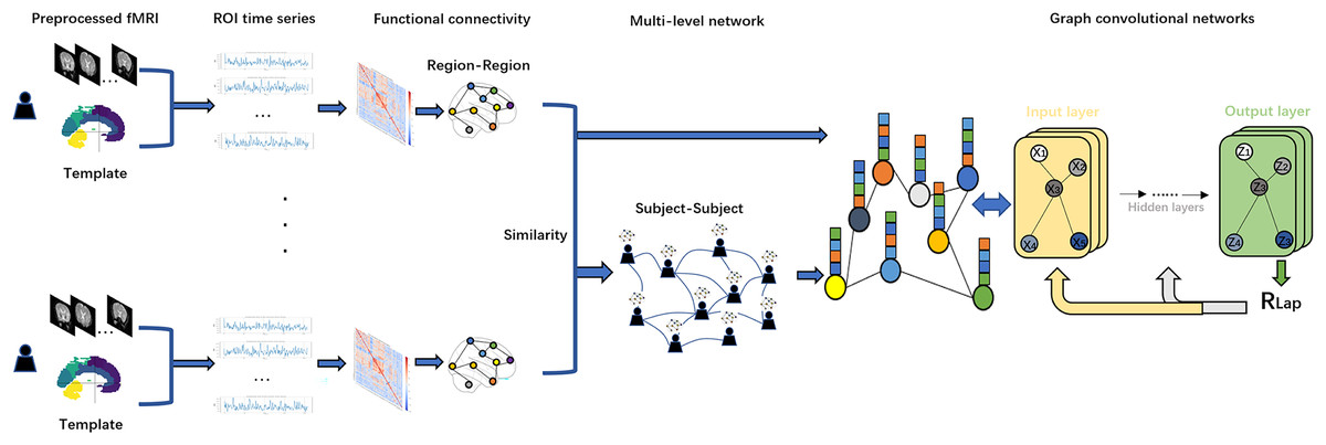
Figure 1: Flowchart of this study.
We first applied Anatomical Automatic Labeling (AAL) brain atlas to the preprocessed fMRI dataset of PD for brain region delineation. Second, time-series data from these brain regions were mapped to regions of interest (ROIs) and functional connectivity (FC) was calculated using Pearson correlation coefficients. Based on the resulting functional connectivity network, a Subject similarity network is further constructed, and the fusion of the two networks constitutes a multi-level network. Finally, we use the functional connectivity matrix with subject-subject similarity matrix as an input to the GCN model for in-depth network analysis. To optimize the model performance and prevent overfitting, we introduce Laplacian regularization (RLap) at the output layer. In addition, we performed an occlusion sensitivity (OS) analysis on the classification results.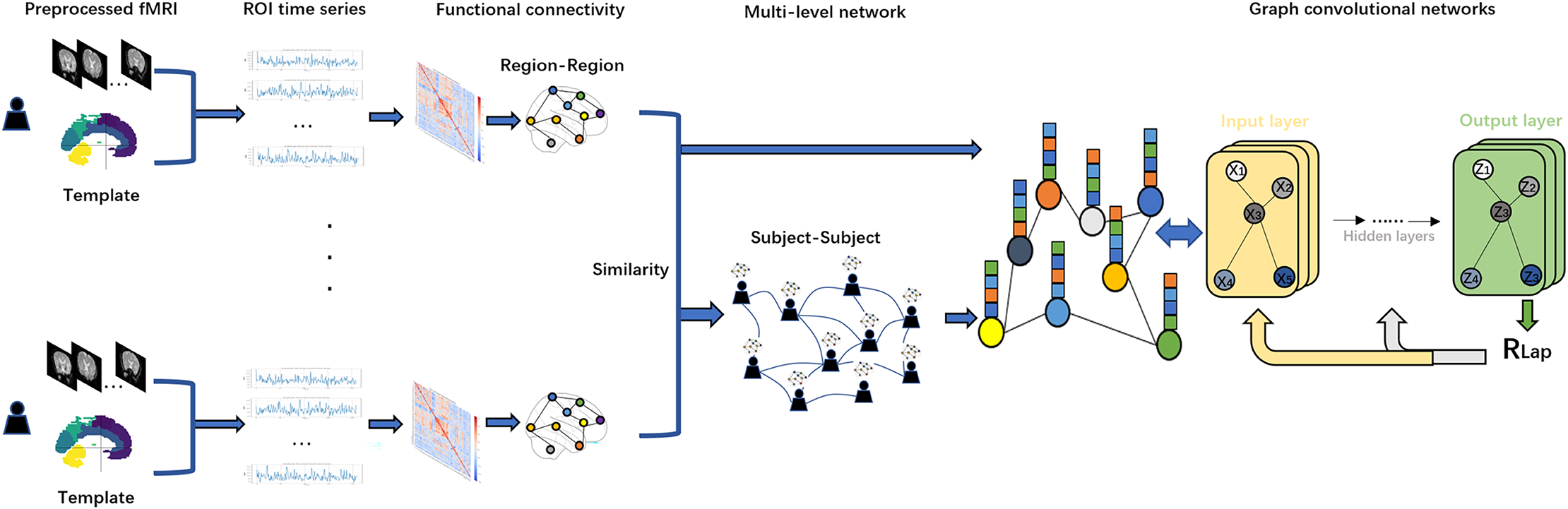
Figure 1 shows a flowchart of this study. In this study, we first use the Anatomical Automatic Labeling (AAL) atlas to parcellate the preprocessed fMRI data of PD patients into distinct brain regions. Second, time-series data from these brain regions are mapped to regions of interest (ROIs) and functional connectivity (FC) is calculated using Pearson correlation coefficients. Based on the resulting functional connectivity network, a subject similarity network is further constructed, and the fusion of the two networks constitutes a multi-level network. Finally, we use the functional connectivity matrix with subject-subject similarity matrix as an input to the GCN model for in-depth network analysis. To optimize the model performance and prevent overfitting, we adopt Laplacian regularization (RLap) at the output layer. In addition, we perform an occlusion sensitivity (OS) analysis on the classification results.
Materials and Methods
Data acquisition and preprocessing PPMI
Neuroimaging data were acquired through the Parkinson’s Progression Markers Initiative (PPMI), a multinational longitudinal study conducted with ethical approval from all participating institutions’ review boards. The data is available at Laboratory of Neuro Imaging (LONI) at the University of Southern California: https://ida.loni.usc.edu/pages/access/search.jsp?tab=collection&project=PPMI; https://www.ppmi-info.org. The data and code is available at GitHub: https://github.com/yangxixi010131/datasetcode. All data were accessed under the PPMI Data Use Agreement. Ethical approval was obtained by PPMI from all participating institutions’ review boards (see PPMI Protocol: https://www.ppmi-info.org/study-design ..%22). The analyzed cohort comprised 103 age- and gender-matched subjects (85 individuals with Parkinson’s disease at the V06 timepoint and 18 healthy controls at V04 baseline) recruited across multiple North American and European clinical centers (Parkinson’s Progression Markers Initiative, 2018). All scans were performed using consistent 3T Siemens MRI systems with harmonized acquisition parameters: repetition time (TR) = 2.4 s, echo time (TE) = 25 ms, flip angle = 80°, isotropic resolution = 3 mm, and variable scan durations (164-210 volumes) based on sequence variants (Table 1).
| Characteristic | PD group (n = 85) | Control group (n = 18) |
|---|---|---|
| Mean age ± SD | 62.3 ± 9.1 yrs | 60.8 ± 10.2 yrs |
| Sex distribution | 54M:31F | 11M:7F |
| Scan protocol | ep2d_RESTING_STATE (n = 44) ep2d_bold_rest (n = 41) |
ep2d_bold_rest (n = 18) |
Table 1. Participant demographics and acquisition parameters. Image processing implemented the Brain Imaging Data Structure (BIDS) specification through fMRIPrep v23.2.1 (Bulcke et al., 2022; Esteban et al., 2019), incorporating temporal slice alignment, motion parameter estimation, and spatial transformation to standard MNI152 space. Whole-brain parcellation into 116 neuroanatomical regions was achieved using the Automated Anatomical Labeling (AAL) template, with subsequent BOLD signal extraction performed via Nilearn’s neuroimaging analysis toolkit (Tzourio-Mazoyer et al., 2002).
Multi-level functional connectivity graph
Individual functional connectivity graph
To quantify the topological characteristics of resting-state brain functional networks, this study constructed individual Static Functional Connectivity (SFC) matrices based on preprocessed BOLD time series. First, the BOLD time series for each subject underwent standardization to eliminate baseline differences across brain regions. The standardization formula is as follows:
(1) where represents the raw time series matrix, denotes the mean vector of time series across brain regions, and 1 is an all-ones row vector.
Subsequently, the Pearson Correlation Coefficient (PCC) (Chen & Yu, 2019) was employed to compute functional connectivity strengths between brain regions, generating a symmetric SFC matrix . For the -th and -th brain regions, their functional connectivity strength is defined as:
(2) where denotes covariance, represents the standard deviation, and ranges within . A larger absolute value indicates stronger functional synergy (Cheng, 2022; Shuai, 2022; Gong et al., 2022; Wang et al., 2014).
Subject-subject functional connectivity graph
To quantify complementary differences in functional connectivity patterns across the patient cohort, this study constructed an inter-subject similarity network based on individual static functional connectivity matrices (Zhu et al., 2018). The specific steps are as follows:
For the static functional connectivity matrices and of the -th and -th subjects, they were first vectorized into one-dimensional feature vectors and . Three similarity functions (Gaussian, Cosine, and Median) were then applied to compute their similarity scores (Liu et al., 2023; Qu et al., 2021):
(3)
(4)
(5) where is the Gaussian kernel bandwidth parameter.
Based on the resulting similarity matrices, we selected the optimal one as the final similarity matrix for network construction, guided by the comparative analysis presented in ‘Parameter Selection for Constructing Subject-Subject Graph’, which identified Gaussian similarity as the best-performing metric. Subsequently, a sparse adjacency matrix was constructed from using the K-nearest neighbor (KNN) algorithm. Each subject retained connections only to its top most similar neighbors, with all other connections set to zero. The elements of the adjacency matrix are defined as:
(6)
To mitigate node degree distribution bias, the adjacency matrix underwent L1 normalization:
(7)
This produced a robust inter-subject similarity network , where represent subjects, and edge weights are defined by the normalized adjacency matrix , providing topological constraints for subsequent graph convolutional network models.
Graph convolutional network
Graph convolutional networks (GCN) have become a key tool for processing graph-structured data (Zhang et al., 2023b; Kingma & Ba, 2014; Li et al., 2021). Unlike conventional neural networks that operate on grid-like inputs, GCNs work directly on topology and node features, yielding superior performance in node-level classification by effectively aggregating neighborhood information (Liu et al., 2023; Ahmedt-Aristizabal et al., 2021). The GCN model takes two inputs: (1) the functional connectivity matrix of subjects as the feature matrix , and (2) the subject-subject similarity matrix as the adjacency matrix . During forward propagation, pass through a Graph Convolution Operation (GCNConv) layer, a BatchNorm layer, a ReLU activation function, a Dropout layer, and finally the output layer. The overall process is shown in Fig. 2. To account for potential confounding effects, we incorporated age and sex as additional covariates in the feature matrix. Specifically, age values were standardized using z-score normalization, while sex was encoded as a binary variable (male = 1, female = 0). These covariates were concatenated with the functional connectivity features prior to model training, ensuring the model could leverage both neuroimaging and demographic information for classification.
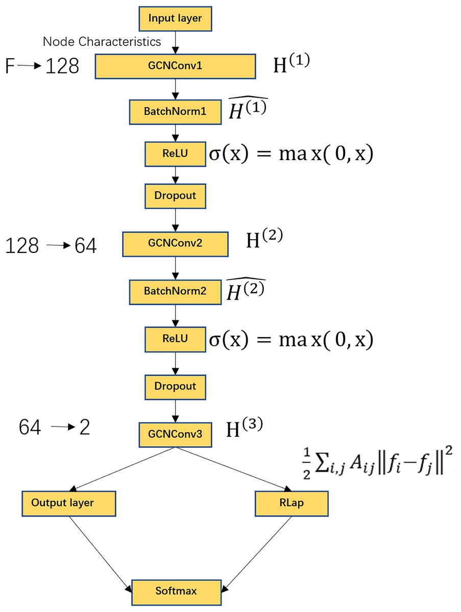
Figure 2: GCN model flowchart.
Includes GCNConv layer, BatchNorm layer, ReLU activation function, Dropout layer, output layer, Laplacian regularization, Softmax activation function. Where F represents the dimension of the receiver node, the input features are converted from F dimensions to 128 dimensions, the second layer of graph convolution, converts the features from 128 dimensions to 64 dimensions, the third layer of graph convolution, outputs the classification score of each node with a dimension of 2. The output layer contains a Softmax function for node classification.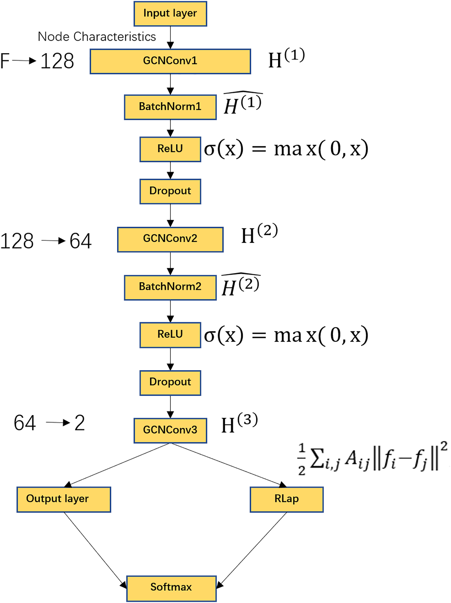
GCNConv data sequentially passes is used to update the node features with the following formula:
(8)
(9)
(10) where denotes the node feature matrix at the l-th layer, denotes the trainable weight matrix of the l-th layer. During training, the model learns the weights by minimizing the loss function. denotes the adjacency matrix of the identity matrix, denotes the unit matrix, plus the unit matrix , denotes the addition of a self-connection, allowing nodes to retain their own features. denotes the degree matrix of , its diagonal is the sum of the corresponding rows of , As a result of the L1 normalization applied in Eq. (7), each row of sums to 1. This is the desired behavior, as it ensures normalized feature propagation and stabilizes the learning process. is the bias term for layer L, denotes the ReLU activation function, which is used to linearity, the formula is .
Batch normalization (BatchNorm) is used to normalize the output of the previous layer to have a mean of 0 and a variance of 1 with the formula:
(11) where μ and are the mean and variance, respectively, of , and are learnable parameters, for scaled and offset normalized data, is a very small constant used to prevent division by zero.
The Dropout operation prevents overfitting by randomly setting a portion of the node features to 0 during training. The ratio of Dropout is over the parameter, usually denoted as p, i.e., the probability that each feature is retained is 1-p. To enhance model generalization and output smoothness, we introduce a Laplacian regularization term to the output layer (Zhu et al., 2018; Qu et al., 2021), defined as follows:
(12) where is the Laplacian regularization matrix, which is given by , and are the feature representations of nodes i and j, respectively.
Laplacian regularized loss function , which is defined as follows:
(13)
, which is defined as follows:
(14) where , which is defined as follows:
(15) where C is the number of categories, is the real label, is the model’s prediction probability that sample i belongs to category c. In the model, supervised learning is used, PD and Control are used as feature labeling information, and 80% of the samples are randomly partitioned into a training set for model training and 20% of the samples are partitioned into a test set for performance evaluation according to the 4 to 1 strategy.
For evaluation, we cite three metrics, classification accuracy, precision, and recall, which are defined as follows:
(16) (17) (18) where represents the number of samples correctly predicted to be in the positive category, represents the number of samples incorrectly predicted to be in the positive category, represents the number of samples correctly predicted to be in the negative category, and represents the number of samples incorrectly predicted to be in the negative category.
The model is trained and tested on a computer with Intel(R) Xeon(R) W-2102 CPU @ 2.90 GHz 2.90 GHz processor, NVIDIA GeForce GTX 2080 TI, 64G RAM, and 64-bit operating system.
Figure 2 shows the schematic of the GCN architecture. The model comprises several key components: a GCNConv layer, a BatchNorm layer, a ReLU activation function, a Dropout layer, an output layer, and Laplacian regularization, followed by a Softmax activation function for final classification. The input node features of dimension F are projected to 128 dimensions in the first graph convolutional layer. A second graph convolution further reduces the feature dimension to 64. The final graph convolutional layer produces a 2-dimensional output, representing the classification logits for each node. The Softmax function in the output layer then converts these logits into class probabilities.
Interpretability of GCN
We categorized 116 ROI brain regions according to lobe delineation criteria based on the AAL brain atlas and identified the functional properties of the relevant lobes using the occlusion sensitivity (OS) analysis (Zeiler & Fergus, 2014; Hu et al., 2019) method. This process not only helps to clarify the interrelationships between the lobes of the brain, but also reveals their importance in a particular cognitive task or neural activity. In our analysis process, the indexing of brain regions within each lobe is first determined, followed by preprocessing of brain functional connectivity matrices and labeling data, followed by construction of graph convolutional network models, and execution of model training and testing. On this basis, lobar obstruction was simulated to assess its effect on model performance. By comparing the difference in accuracy before and after the blockage, box plots were drawn using Seaborn to visualize the effect of blockage in different brain regions on classification accuracy. This allows for a direct assessment of the importance of each lobe to the model’s performance in identifying PD, providing a tool to understand their specific roles in the classification task. This systematic analysis provides insights into the organization of functional networks in Parkinson’s disease. The identified lobe-specific roles offer valuable evidence to aid in understanding the neural mechanisms underlying PD and may inform the development of future neuroimaging-based diagnostic tools (Yan et al., 2020; Chen et al., 2024; Li et al., 2024; Ma, 2024; Mao, 2024).
Results
Functional connectivity graph of individuals
This study employed Gaussian similarity analysis to visualize resting-state functional connectivity networks in three PD patients (Fig. 3). The results demonstrated marked heterogeneity in prefrontal-sensorimotor network connectivity patterns: Subject 1 exhibited stronger prefrontal-parietal connections (darker edges), while Subjects 20 and 100 displayed enhanced fronto-occipital coupling. Although limited by sample size, these preliminary observations reveal individualized characteristics of functional network reorganization in PD, establishing a methodological framework for future large-scale investigations.
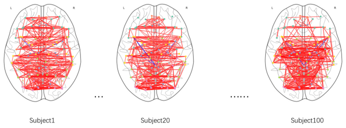
Figure 3: Functional brain connectivity networks in axial view.
Darker colors indicate stronger connectivity.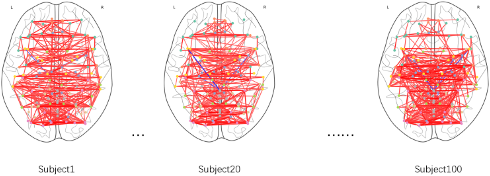
Parameter selection for constructing subject-subject graph
Selection of K value
To systematically evaluate the impact of the K value (the number of nearest neighbors retained for each node in the subject-subject similarity network) on model performance, this experiment was conducted under fixed hyperparameter conditions (including the Gaussian similarity function, learning rate of 0.01, and weight decay of 1e−4), with the Laplacian regularization parameter (λ) set to 0 to eliminate its interference in the K-value sensitivity analysis. We tested multiple parameter values at intervals of 10 within the range of K = 10 to 100 (i.e., K = 10, 20, 30, …, 100). As shown in Fig. 4, when K increased from 10 to 20, the model performance improved significantly (accuracy increased from 73.3% to 75.2%). However, as K continued to increase beyond 20 (K > 20), the performance exhibited a gradual decline. This phenomenon suggests that smaller K values may lead to loss of effective information due to overly sparse graph structures, while excessively large K values introduce redundant connections that accumulate noise. Therefore, K = 20 was selected as the optimal parameter, achieving the best balance between sparsity and information completeness.
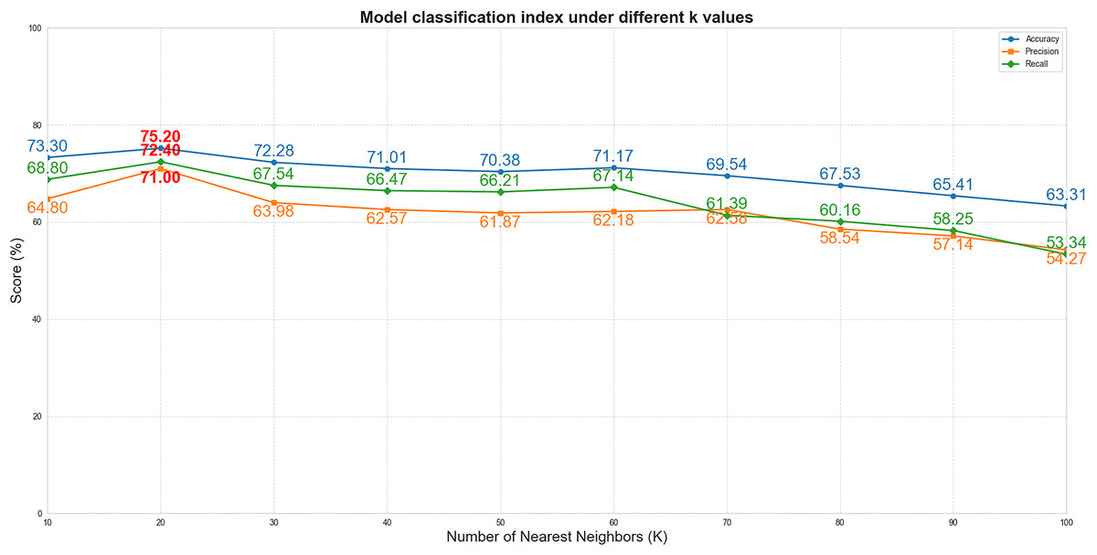
Figure 4: The performance curves of the model vs. different K values.
(The x-axis represents K values, and the y-axis represents percentages). The blue, orange, and green curves correspond to accuracy, precision, and recall, respectively.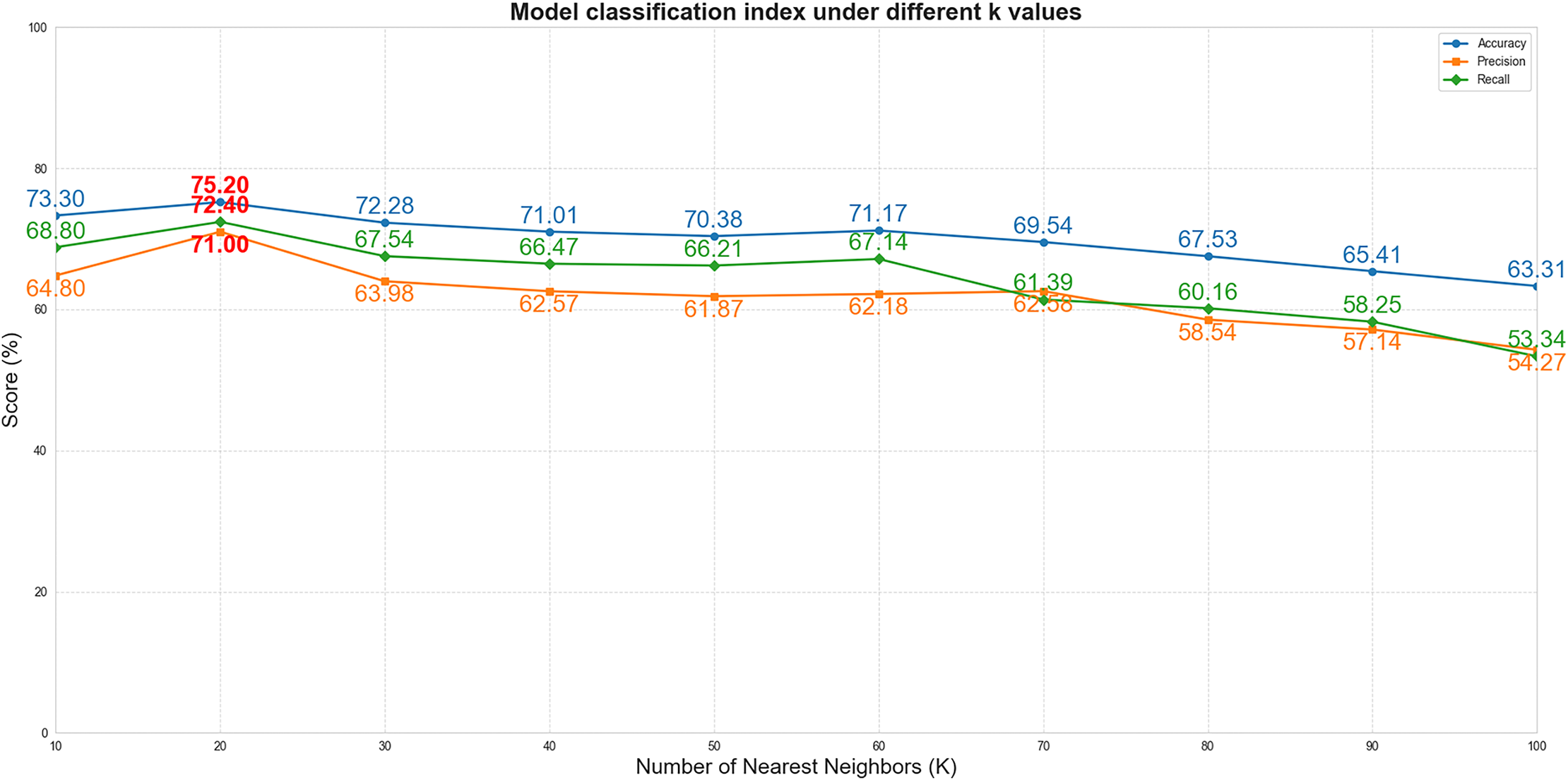
Selection of similarity function
In our algorithm implementation, we introduced three different similarity measures—Cosine similarity, Median similarity, and Gaussian similarity—and evaluated them with the K value uniformly set to 20. Although the edge weight distributions of these functions show considerable overlap in Fig. 5, we selected the Gaussian similarity for two primary reasons. First, its exponential kernel is theoretically well-suited for capturing nonlinear relationships in the functional connectivity feature space. Second, and more critically, in our experimental validation, it consistently achieved the highest classification accuracy among the three candidates. Therefore, the Gaussian similarity function was adopted for our final model.
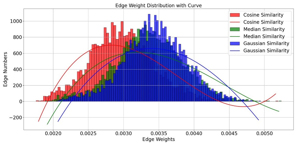
Figure 5: Edge weight distribution with curve.
Edge distribution performance for different similarity functions.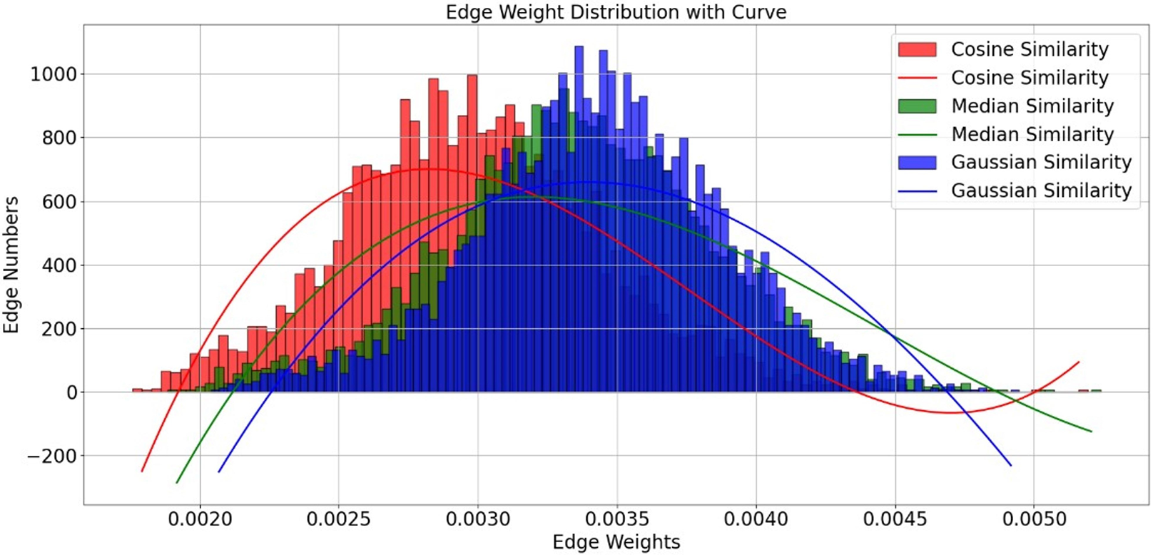
Selection of λ value
To systematically evaluate the impact of the Laplacian regularization parameter (λ) on model performance, we conducted experiments with λ values ranging from 0.05 to 0.25 at intervals of 0.05. All other hyperparameters remain fixed. As illustrated in Fig. 6, model performance exhibited a clear dependency on λ. When λ increased from 0.05 to 0.1, classification accuracy improved from 74.14% to 76.2%, precision from 70.1% to 72.22%, and recall from 72.47% to 75.3%. This indicates that introducing Laplacian regularization effectively mitigates overfitting and enhances feature representation by leveraging graph structure constraints. However, further increasing λ beyond 0.1 led to performance degradation, with accuracy dropping to 59.81% at λ = 0.25. This trend suggests that excessive regularization overly constrains the model, suppressing its ability to learn discriminative features. The optimal balance between generalization and model flexibility was achieved at λ = 0.1, which maximized all evaluation metrics. These results underscore the critical role of Laplacian regularization in stabilizing training and improving classification robustness, particularly in small-sample fMRI datasets.
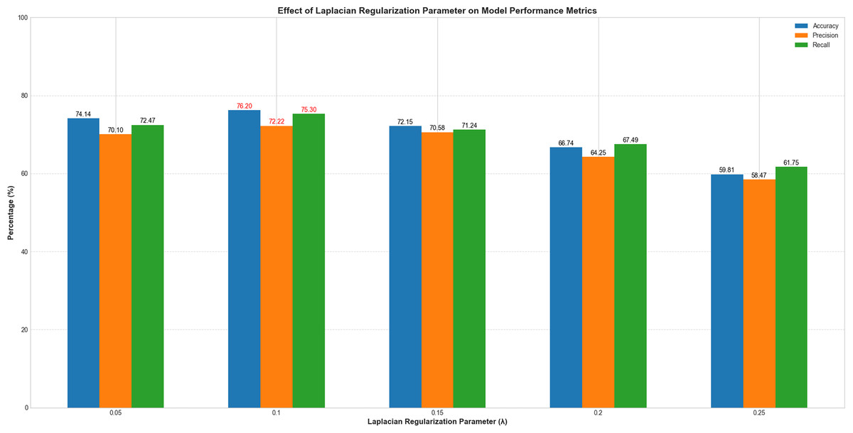
Figure 6: Performance variation with Laplacian regularization parameter (λ).
The x-axis represents λ values (0.05–0.25), and the y-axis denotes evaluation metrics (%). Blue, orange, and green curves correspond to accuracy, precision, and recall, respectively.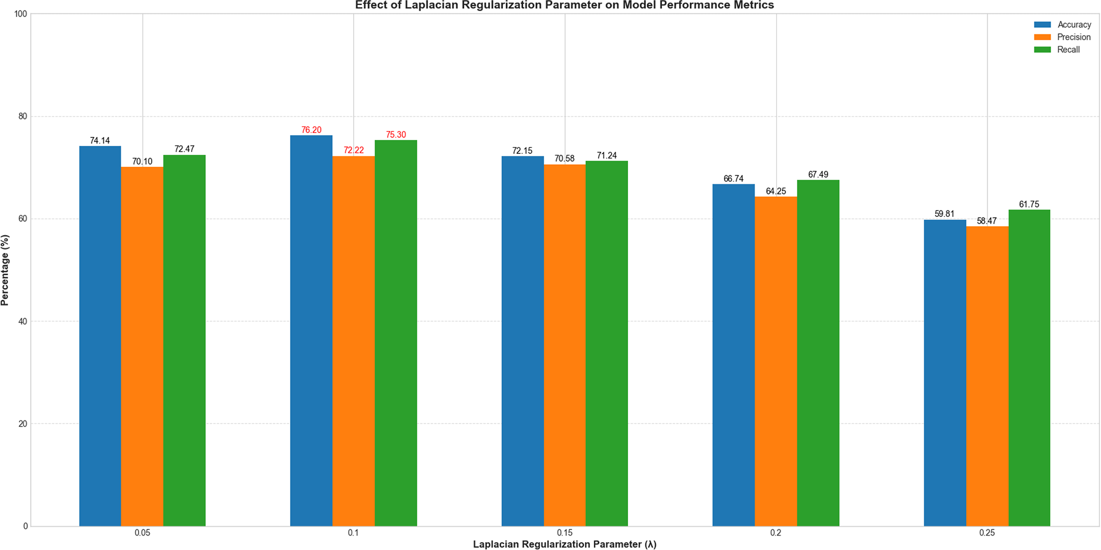
Subject-subject graph
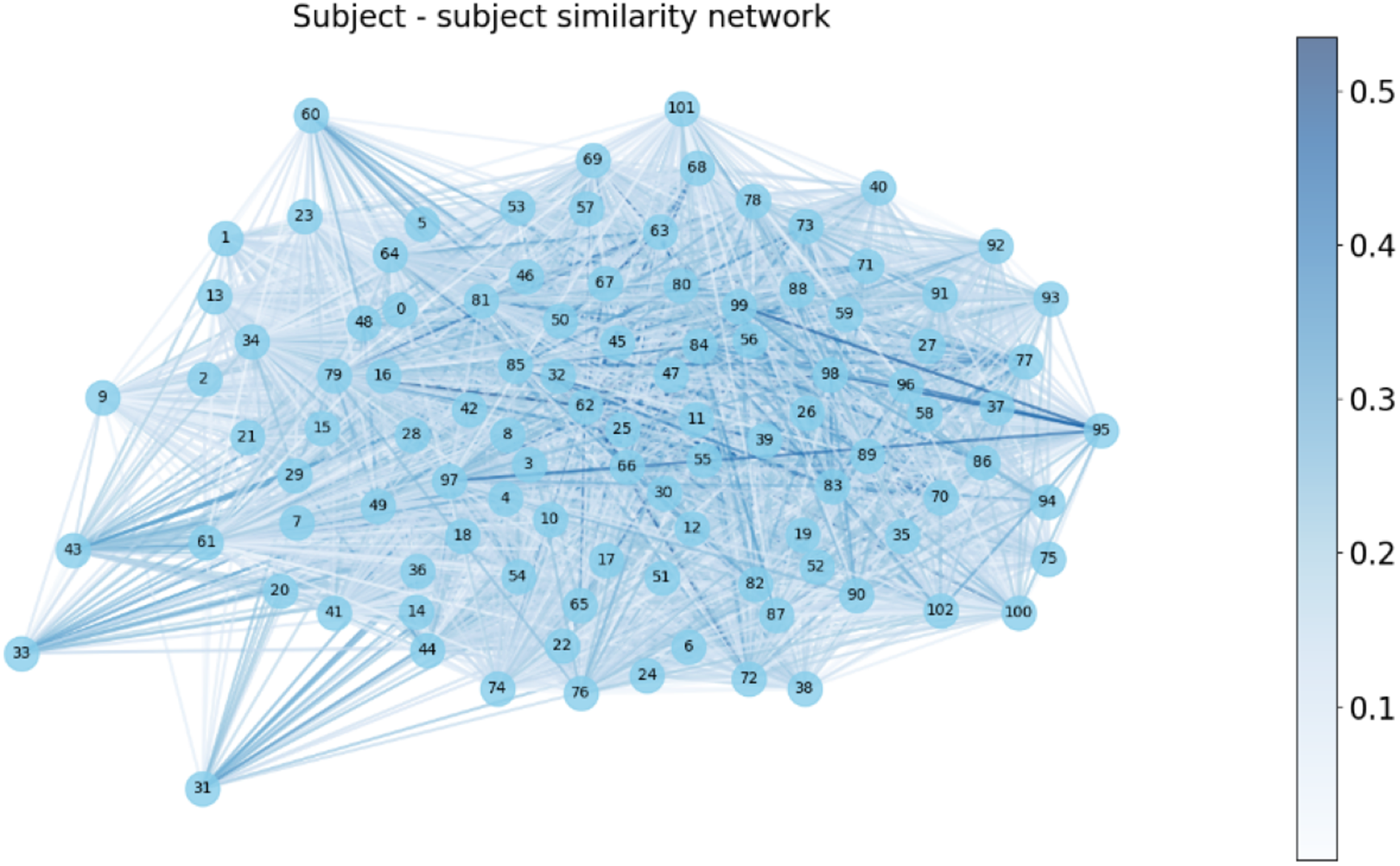
We constructed a subject-subject similarity network by evaluating the functional connectivity (FC) similarity between subjects in Fig. 7. In this network, each subject corresponds to a vertex and the edges represent the similarity between subjects. The weights of the edges are indicated by the shade of the color, with darker colors indicating higher similarity and lighter colors indicating lower similarity.
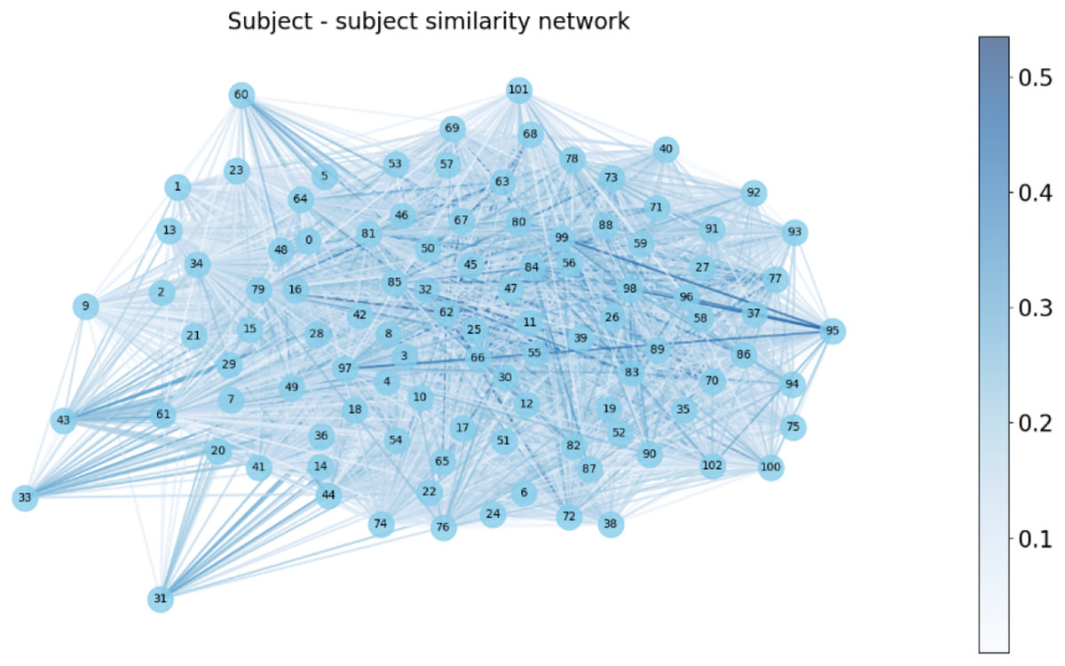
Figure 7: Subject-subject similarity network.
Model performance evaluation
Hyperparameter selection of GCN
To ensure the robustness and generalizability of our GCN model, we employed a rigorous hyperparameter tuning strategy combining empirical validation and grid search. The model architecture was optimized through systematic experimentation. We evaluated networks with 2–4 graph convolutional layers and found that a 3-layer structure (128-64-2 channels) achieved the best balance between model complexity and performance (as detailed in Table 2), as deeper networks tended to overfit on our limited fMRI dataset. Among Gaussian, Cosine, and Median similarity metrics, Gaussian similarity yielded superior results due to its ability to capture nonlinear relationships in FC data. For the subject-subject similarity network, we tested KNN with K ∈ [10, 100] in increments of 10, identifying K = 20 as the optimal value that balanced sparsity and connectivity density, as shown in Table 2. The Laplacian regularization strength (λ) was fine-tuned within the range [0.05, 0.25], with λ = 0.1 providing the best trade-off between preventing overfitting and preserving discriminative power (Table 2). We used the Adam optimizer with a multi-stage learning rate decay (0.01, 0.005, 0.001) and applied weight decay (1e−4) and dropout (p = 0.01) to enhance generalization. Due to the small sample size (N = 103), we initially performed stratified 5-fold cross-validation to ensure stability before finalizing the 80–20 train-test split (stratified by class). All experiments were repeated five times with different random seeds to mitigate variability, and the reported metrics reflect mean performance across runs.
| Hyperparamter | Value |
|---|---|
| Optimizer | ADAM |
| Layers | 3 |
| Channels | [128, 64, 2] |
| Similarity function | Gaussian |
| K-value | 20 |
| Activation function | [ReLu, ReLu, Softmax] |
| Learning rate | 0.01 |
| Weight decay | 1e−4 |
| λ (RLap parameter) | 0.1 |
| Epochs | 100 |
Performance evaluation of GCN
In the experiments, we compared two scenarios: one using the patient similarity network and the other without it (i.e., employing a fully connected graph where K = N − 1). The results demonstrated that the classification accuracy of the model significantly improved when the patient similarity network was incorporated. Specifically, the GCN model utilizing the patient similarity network achieved a classification accuracy of 76.2%, whereas the GCN model with a fully connected graph attained only 66.7% accuracy (Table 3). These findings indicate that the patient similarity network effectively captures complementary features of inter-individual functional connectivity, thereby enhancing the model’s discriminative capability. By leveraging similarity information among patients, the model can more efficiently identify patient groups with shared pathological characteristics, ultimately improving classification accuracy.
| Model | Accuracy | Precision | Recall |
|---|---|---|---|
| GCN (K = 20) | 0.762 | 0.722 | 0.753 |
| GCN (K = N − 1) | 0.667 | 0.5 | 0.413 |
Model comparison
To comprehensively evaluate the performance and generalization capability of the constructed GCN model for PD classification, this study conducted systematic comparisons with several benchmark models: Support Vector Machine (SVM), Multi-Layer Perceptron (MLP), Graph Attention Network (GAT), and Graph Transformer (GT). Models were trained and tested on both the original PPMI dataset (n = 103) and an external validation set derived from the Human Connectome Project (HCP) database (n = 50; comprising 30 prodromal PD patients from PPMI and 20 healthy controls from HCP; source: https://db.humanconnectome.org). All models utilized the same datasets under an identical evaluation protocol, employing an 80/20 training/testing split. Under dual validation using both the primary PPMI dataset and the external HCP validation set, the constructed GCN model (with and without Laplacian regularization) consistently outperformed the benchmark models across three key metrics: classification accuracy, precision, and recall (Table 4). These findings demonstrate that the GCN model effectively leverages node features and relational structures to capture underlying data patterns, exhibiting superior performance for PD classification tasks. The model’s strength lies in its ability to simultaneously aggregate local interactions between brain regions and global patient relationships, thereby fully utilizing the graph-structured information inherent in functional connectivity networks and patient similarity networks. This approach provides robust support for the early diagnosis of neurodegenerative disorders. The performance disparity among models can be attributed to their differing inductive biases and capacities relative to our dataset size. The SVM model, while robust, may compromise the inherent spatial topology by flattening the functional connectivity matrix into a feature vector. More importantly, the GAT and GT models, with their large number of parameters, are likely challenged by the limited sample size, potentially leading to underfitting as they struggle to effectively learn generalized patterns from the scarce data. This highlights a key limitation of applying highly complex architectures to small-scale neuroimaging datasets without leveraging pre-training.
| Primary cohort | External hybrid validation | |||||
|---|---|---|---|---|---|---|
| Model | Accuracy | Precision | Recall | Accuracy | Precision | Recall |
| SVM | 0.71 | 0.5 | 0.25 | 0.65 | 0.52 | 0.36 |
| MLP | 0.741 | 0.644 | 0.741 | 0.7 | 0.72 | 0.75 |
| GAT | 0.72 | 0.405 | 0.5 | 0.63 | 0.39 | 0.52 |
| GT | 0.714 | 0.649 | 0.728 | 0.705 | 0.69 | 0.71 |
| GCN(λ = 0) | 0.741 | 0.701 | 0.725 | 0.73 | 0.691 | 0.667 |
| GCN(λ = 0.1) | 0.762 | 0.722 | 0.753 | 0.75 | 0.746 | 0.708 |
Interpretability of classification
We utilized occlusion sensitivity (OS) analysis (Zeiler & Fergus, 2014; Hu et al., 2019) to identify the functional properties of specific lobes, and we categorized the 116 ROIs into the frontal, occipital, parietal, subcortical, temporal, and cerebellum lobes based on their unraveling location. Of these, Frontal contained 32 ROIs, Occipital contained 12 ROIs, Parietal contained 16 ROIs, Subcortical contained 10 ROIs, Temporal contained 20 ROIs, and Cerebellum contained 26 ROIs. The classification accuracies derived from the GCN model in different cases of lobar obstruction, and thus inferring which lobes play to important roles, are shown in Fig. 8. If classification accuracy is maintained at a high level, this suggests that the blocked lobes have a limited effect on the classification task; conversely, if classification accuracy decreases significantly, this suggests that the blocked lobes have an important role to play in accomplishing the classification task. As can be seen from the figure the frontal lobe plays an important role in classification. Figure 9 represents the average occlusion sensitivity at the ROI level in different brain lobes. To see the functional connectivity of each lobe more clearly, we also visualized the brain function connectivity network in coronal, sagittal, and axial views, respectively, as shown in Fig. 10.
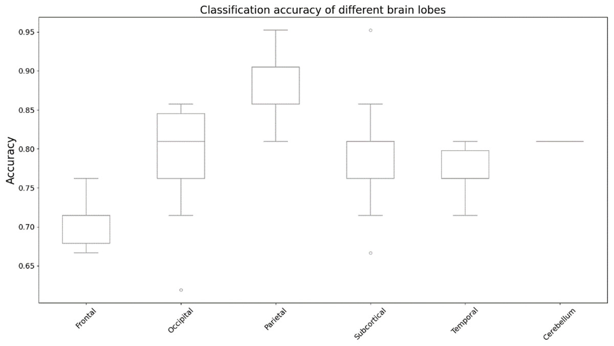
Figure 8: Classification accuracy of different brain lobes.
Results of altered accuracy by blocking different lobes of the brain.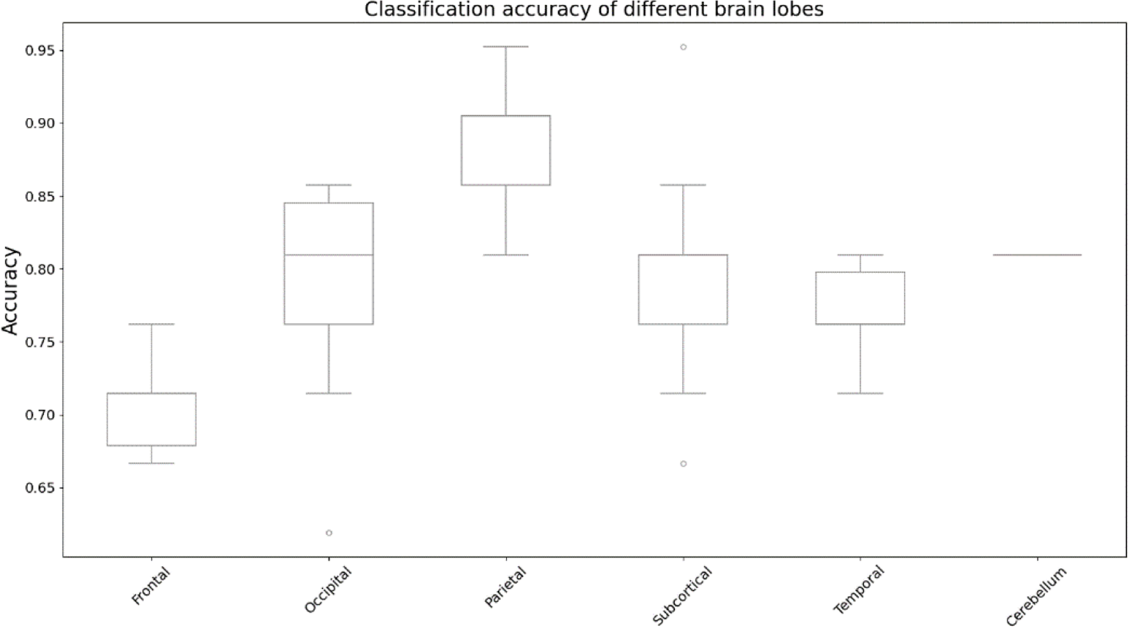
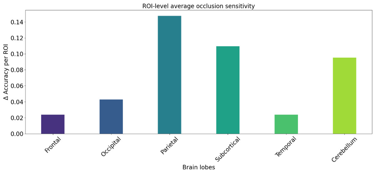
Figure 9: ROl-level average occlusion sensitivity.
Mean occlusion sensitivity of ROI levels in different lobes of the brain.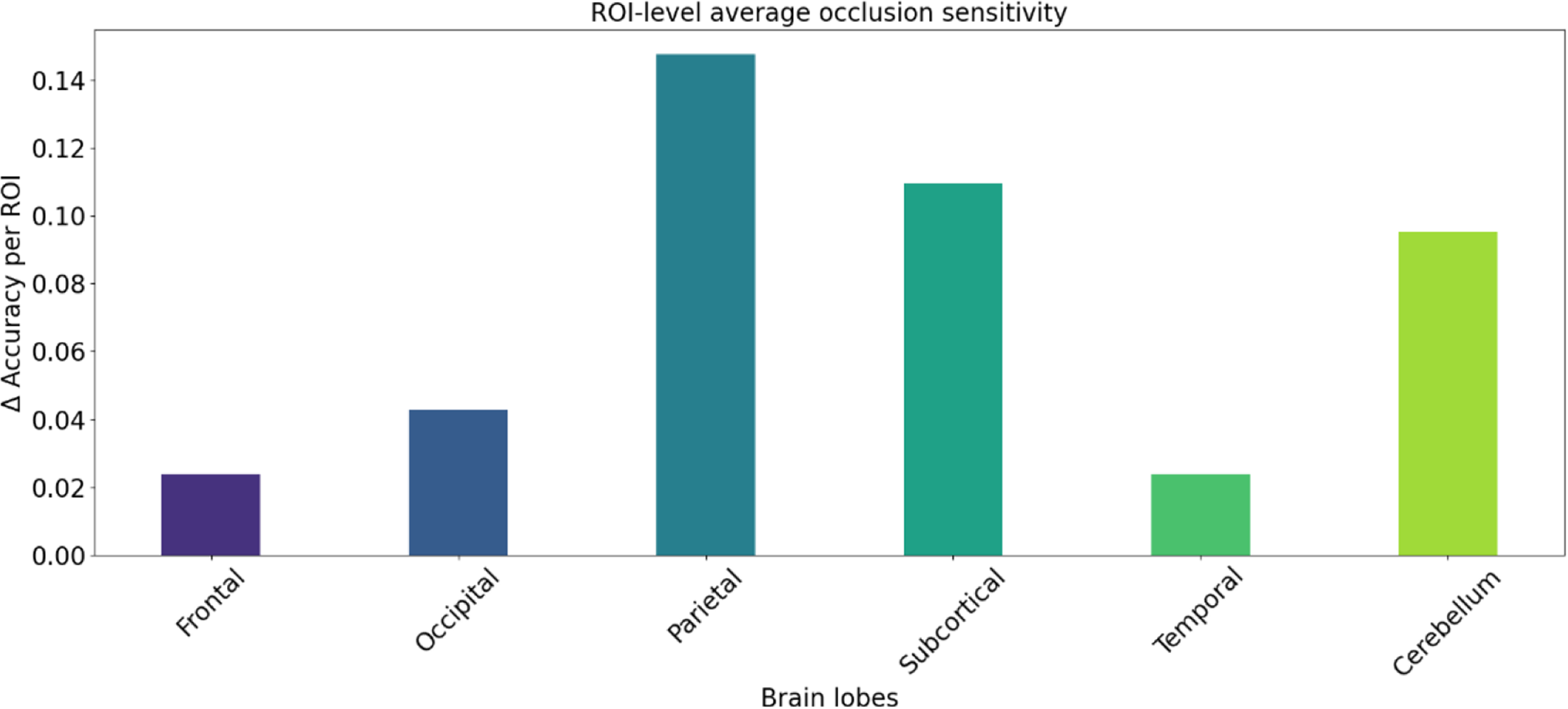
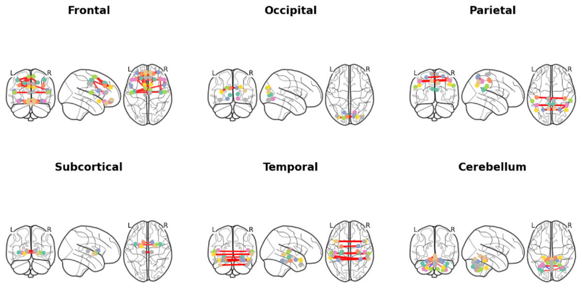
Figure 10: Brain functional connectivity networks of different brain lobes in coronal, sagittal and axial positional views.
Different colored lines identify specific functional connection paths: red and yellow lines in the frontal area highlight major functional connections; The green lines in the occipital lobe area identify key connections in the visual processing area; The red lines in the parietal lobes show the connections between sensory integration areas; The yellow lines in the subcortical area mark the major connections associated with motor control; The red lines in the temporal lobe region highlight key connections between auditory and language processing areas; The red line in the cerebellar region identifies the major connections associated with coordinated movement. These color codes help identify different types and strengths of connections, which reveals a complex network of interactions between different regions within the brain.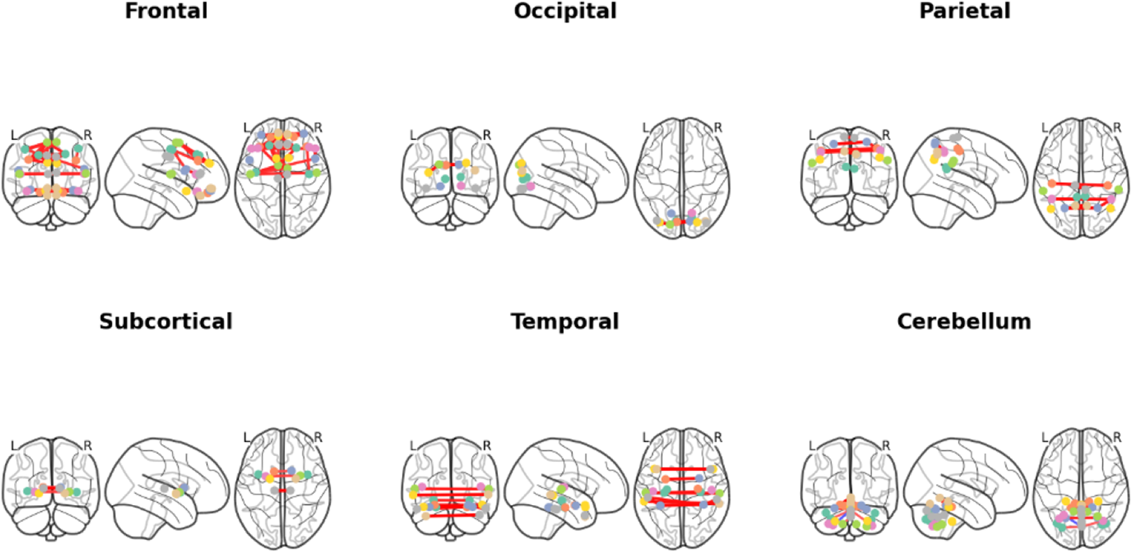
Discussion
In our study, based on the results of Parameter selection for constructing subject-subject graph in ‘Results’, K value of 20 and Gaussian similarity function are chosen as the adjacency matrix of subject-subject similarity matrix. This result not only highlights the importance of k-value selection for similarity computation, but also provides a key parameter reference for subsequent studies, where the edge weights computed when using Gaussian similarity have a stronger distinguishing ability. The subject-subject similarity network generated based on subject-subject similarity matrix can clearly show the similarity intensity between different subjects and intuitively reflect the relationship and similarity distribution among subjects. It is crucial that the introduction of the patient similarity network addresses a key limitation of traditional FC-based PD diagnosis methods (Qu et al., 2021). These methods mainly focus on FC patterns within individual patients, largely overlooking the valuable information contained in the similarity of FC patterns between patients. Specifically, this network-level perspective supplements individual FC networks by leveraging group structure information, guiding the GCN to learn robust and disease-state-representative features across subjects. By explicitly modeling patient relationships based on FC similarity, the patient similarity network enables the GCN model to aggregate information not only from interactions between local brain regions within a single subject but also from globally similar subjects. This dual aggregation mechanism enables the model to leverage complementary information: individual FC captures the patient’s unique brain connectivity topology, while the patient similarity network informs the model of the patient’s relationship to other patients in the cohort, highlighting shared pathological features. Consequently, the patient similarity network contributes significantly to enhancing the model’s generalization ability and achieving higher classification accuracy, precision, and recall rates.
From the results of model performance evaluation, the use of Laplacian regularization (λ = 0.1) is the best solution, and the introduction of Laplacian regularization effectively solves the overfitting problem on the dataset, in addition to a comprehensive comparison analysis of the GCN model and other models’ performance is comprehensively compared and analyzed. The results show that the GCN model performs well in all evaluation metrics, especially after the introduction of Laplacian regularization, its performance is significantly improved. This result shows that the GCN model can effectively capture potential features when dealing with node features and inter-node relationships, thus significantly improving the classification performance and verifying its superiority and applicability in related tasks. In order to determine which brain lobes play a key role in the categorization task, we performed an OS analysis of individual brain lobes. The analysis showed that the frontal lobe played a significant role in the classification process. This analysis not only reveals the variability in connectivity patterns across brain lobes, but also provides new insights into deeper understanding of the brain’s functional networks. These findings are consistent with those of Qu et al. (2021).
There are some limitations to our experiments; first, the number of subjects in our dataset is relatively small, and although we introduced Laplacian regularization to effectively mitigate the overfitting problem on the dataset, the sample size is still small. This limitation may lead to a reduction in computational complexity, which may adversely affect the various performance metrics of the model. Insufficient sample size may affect the generalization ability and stability of the model, making the assessment metrics not adequately reflect the performance of the model on a larger sample. Therefore, future studies should consider enlarging the sample size to improve the representativeness of the data and the reliability of the model, so as to enhance the credibility and generalizability of the findings. Second, we only studied static functional connectivity and did not consider the impact of dynamic functional connectivity. While studies conducted in the resting state provide important insights, it is worth noting that functional connectivity (FC) in the brain is actually a dynamic process that changes over time. This dynamic characterization may reflect the brain’s ability to adapt under different cognitive tasks and states. Therefore, future studies should integrate the analysis of dynamic functional connectivity for a more comprehensive understanding of the time-varying properties of brain networks and their role in cognitive functions (Kudela, Harezlak & Lindquist, 2017; Wang, Wang & Lan, 2019).
Conclusions
In this study, we focused on addressing differences and complementarities in functional connectivity between individuals that have not been adequately accounted for by traditional approaches in PD diagnosis. For this reason, this article constructs a patient similarity network based on FC and combines it with patient FC to form a multilayer network, which utilizes the GCN model to efficiently deal with the complex graph-structured data of FC and patient similarity network. The GCN model performs well in PD diagnosis with 76.2% classification accuracy, 72.2% precision, and 75.3% recall, all of which outperform other benchmark models, demonstrating its superior performance in graph-structured data classification. Furthermore, through OS analysis, we found that the frontal lobe plays a key role in the classification task, highlighting its importance in model classification. The method used in this article is not only able to deeply mine the complex associations in brain structure data, but also provides strong support for understanding the cognitive functions of the brain and revealing the interaction mechanisms between brain regions and individuals.