
Faster numeric static analyses with unconstrained variable oracles
- Published
- Accepted
- Received
- Academic Editor
- Marieke Huisman
- Subject Areas
- Algorithms and Analysis of Algorithms, Theory and Formal Methods, Software Engineering
- Keywords
- Abstract interpretation, Static analysis, Abstract compilation, Unconstrained variables
- Copyright
- © 2025 Arceri et al.
- Licence
- This is an open access article distributed under the terms of the Creative Commons Attribution License, which permits unrestricted use, distribution, reproduction and adaptation in any medium and for any purpose provided that it is properly attributed. For attribution, the original author(s), title, publication source (PeerJ Computer Science) and either DOI or URL of the article must be cited.
- Cite this article
- 2025. Faster numeric static analyses with unconstrained variable oracles. PeerJ Computer Science 11:e3390 https://doi.org/10.7717/peerj-cs.3390
Abstract
In the context of static analysis based on abstract interpretation, we propose a lightweight pre-analysis step which is meant to suggest, at each program point, which program variables are likely to be unconstrained for a specific class of numeric abstract properties. Using the outcome of this pre-analysis step as an oracle, we simplify the statements of the program being analyzed by propagating this lack of information, aiming at fine-tuning the precision/efficiency trade-off of the target static analysis. A thorough experimental evaluation considering real world programs shows that the idea underlying the approach is promising. We first discuss and evaluate several variants of the pre-analysis step, measuring their accuracy at predicting unconstrained variables, so as to identify the most effective ones. Then we evaluate how these pre-analyses affect the target static analysis, showing that they can improve the efficiency of the more costly analysis while having a limited effect on its precision.
Introduction
Static analyses based on abstract interpretation (Cousot & Cousot, 1977) correctly approximate the collecting semantics of a program by executing it on an abstract domain modeling the properties of interest. In the classical approach, which follows a pure program interpretation scheme, the concrete statements of the original program are abstractly executed step by step, updating the abstract property describing the current program state: while being correct, this process may easily incur avoidable inefficiencies and/or precision losses. To mitigate this issue, static analyzers sometimes apply simple, safe program transformations that are meant to better tune the trade-off between efficiency and precision. For instance, when trying to improve efficiency, the evaluation of a complex nonlinear numeric expression (used either in a conditional statement guard or as the right hand side expression in an assignment statement) may be abstracted into a purely nondeterministic choice of a value of the corresponding datatype; in this way, the overhead incurred to evaluate it in the considered abstract domain is avoided, possibly with no precision loss, since its result was likely imprecise anyway. On the other hand, when trying to preserve precision, a limited form of constant propagation may be enough to transform a nonlinear expression into a linear one, thereby allowing for a reasonably efficient and precise computation on commonly used abstract domains tracking relational information. As another example, some tools apply a limited form of loop unrolling (e.g., unrolling the first iteration of the loop (Blanchet et al., 2003)) to help the abstract domain in clearly separating those control flows that cannot enter the loop body from those that might enter it; this transformation may trigger significant precision improvements, in particular when the widening operator is applied to the results of the loop iterations.
Sometimes, the program transformations hinted above are only performed at the semantic level, without actually modifying the program being analyzed; hence, the corresponding static analysis tools can still be classified as pure program interpreters. However, in principle the approach can be directly applied at the syntactic level, so as to actually translate the original program into a different one, thereby moving from a pure program interpretation setting to a hybrid form of (abstract) compilation and interpretation. Note that the term Abstract Compilation, introduced in Hermenegildo, Warren & Debray (1992), Warren, Hermenegildo & Debray (1988), sometimes has been understood under rather constrained meanings: for instance, Giacobazzi, Debray & Levi (1995) and Amato & Spoto (2001) assume that the compiled abstract program is expressed in an existing, concrete programming language; Boucher & Feeley (1996) and Wei, Chen & Rompf (2019) focus on those inefficiencies that are directly caused by the interpretation step, without considering more general program transformations. Here we adopt the slightly broader meaning whereby portions of the approximate computations done by the static analysis tool are eagerly performed in the compilation (i.e., program translation) step and hence reflected in the abstract program representation itself. Clam/Crab (Gurfinkel & Navas, 2021) and IKOS (Brat et al., 2014) are examples of tools adopting this hybrid approach for the analysis of LLVM bitcode, leveraging specific intermediate representations designed to accommodate several kinds of abstract statements. A similar approach is adopted in LiSA (Ferrara et al., 2021; Negrini et al., 2023), to obtain a uniform program intermediate representation when analyzing programs composed by modules written using different programming languages.
Article contribution. Adopting the abstract compilation approach, we propose a program transformation that is able to tune the trade-off between precision and efficiency. The transformation relies on an oracle whose goal is to suggest, for each program point, which program variables are likely unconstrained for a target numeric analysis of interest. By systematically propagating the guessed lack of information, the oracle will guide the program transformation so as to simplify those statements of the abstract program for which the target analysis is likely unable to track useful information.
We model our oracles as pre-analyses on the abstract program, considering two Boolean parameterizations and thus obtaining four possible oracle variants: we will have non-relational or relational numeric analysis oracles and each of them can be existential or universal. The proposed program transformation can be guided by any one of these variants, allowing different degrees of program simplification, thereby obtaining different trade-offs between the precision and the efficiency of the target analysis. It is important to highlight that the oracles we are proposing have no intrinsic correctness requirement; as we will discuss in ‘Detecting Likely Unconstrained Variables’, whatever oracle is adopted to guess the set of unconstrained variables, its use will always result in a sound program transformation. The (im-)precision of the oracle guesses can only affect the precision and efficiency of the target numeric analysis: aggressive oracles, which predict more variables to be unconstrained, will result in faster but potentially less precise analyses; conservative oracles, by predicting fewer unconstrained variables, will result in slower analyses, potentially preserving more precision.
Our proposal will be experimentally evaluated on a set of 30 Linux drivers taken from the SV-COMP repository. We will test the four oracle variants on these benchmarks, considering as target analyses the classical numeric analyses using the abstract domains of intervals and convex polyhedra. In our experimental evaluation, we will pursue two different goals: first, we will provide a thorough assessment of the accuracy of the four oracle variants, checking their ability to correctly predict if a numeric program variable is unconstrained when using a specific target analysis; then, we will measure the effectiveness of the program transformation step at affecting the trade-off between precision and efficiency of the target static analyses, so as to identify the most promising oracle variant and the contexts where its use is beneficial.
Article structure. In ‘Preliminaries’ we briefly and informally introduce the required concepts and notations used in the rest of the article. In ‘Detecting Likely Unconstrained Variables’, after introducing the notion of likely unconstrained variable for a target numeric analysis, we define four different oracles as variants of a dataflow analysis tracking variable unconstrainedness; we also formalize the program transformation that, guided by these oracles, simplifies the abstract program being analyzed. The design and implementation of our experimental evaluation are described in ‘Implementation and Experimental Evaluation’, where we also provide an initial measure of how often the program transformation affects the code under analysis. In ‘Assessing the Accuracy of LU Oracles’ we discuss in greater detail, also by means of simple examples, the reasons why the predictions of the oracles defined in ‘Detecting Likely Unconstrained Variables’ could give rise to both false positives and false negatives; we then provide an experimental evaluation assessing their accuracy on the considered benchmarks. In ‘Precision and Efficiency of the Target Analyses’ we evaluate the effect of the program transformation on the target numerical analyses: we first focus on a precision comparison and then on an efficiency comparison, so as to reason on the resulting trade-off. Related work is discussed in ‘Related Work’, while ‘Conclusion’ concludes, also describing future work. When describing and discussing the results of our experiments in ‘Implementation and Experimental Evaluation’, ‘Assessing the Accuracy of LU Oracles’ and ‘Precision and Efficiency of the Target Analyses’, we will often summarize experimental data using descriptive statistics and/or accuracy metrics; the corresponding detailed tables are provided in the Appendix.
This article is a revised and extended version of Arceri, Dolcetti & Zaffanella (2023b). First, we added some background material in ‘Preliminaries’, so as to enhance its readability. We also extended the main experimental evaluation by considering a larger set of real-world test cases. The main extension is in ‘Assessing the Accuracy of LU Oracles’, where we provide an in depth analysis of the accuracy of the oracles we are proposing to detect likely unconstrained variables, showing simple examples witnessing both false positives and false negatives and explaining their origin; this qualitative analysis is complemented with a corresponding experimental evaluation providing a quantitative assessment of the accuracy of the oracles on the considered benchmarks.
Preliminaries
Assuming some familiarity with the basic notions of lattice theory, in this section we briefly recall some basic concepts of abstract interpretation (Cousot & Cousot, 1977, 1979), as well as the well known domains of intervals (Cousot & Cousot, 1977) and convex polyhedra (Cousot & Halbwachs, 1978); non-expert readers are also referred to Miné (2017) for a complete tutorial on the inference of numeric invariant properties using Abstract Interpretation.
Abstract interpretation The semantics of a program can be specified as the least fixpoint of a continuous operator defined on the concrete domain C, often formalized as a complete lattice . The partial order relation models the approximation ordering, establishing the relative precision of the concrete properties. The least fixpoint can be obtained as the limit of the increasing chain of Kleene’s iterates, defined by and , for . Static analyses based on Abstract Interpretation aim at computing a sound approximation of the concrete semantics by using a simpler abstract domain A, usually formalized as a bounded join semi-lattice : the relative precision of the abstract elements is encoded by the abstract partial order , mirroring the concrete one. Intuitively, the goal is to mimic the concrete semantics construction by providing an abstract semantics operator and computing a corresponding increasing chain of abstract Kleene’s iterates , where and , converging to an abstract element that correctly approximates the concrete fixpoint.
The relation between the concrete and abstract domains is often formalized using a monotonic concretization function , which maps each abstract element into its corresponding concrete meaning. An abstract semantics function is a correct approximation of the concrete function if and only if for all . When the concrete and abstract domains can be related by a Galois connection, one can define a corresponding abstraction function satisfying
in such a context, each concrete semantics function can be matched by its best correct approximation ; however, there are cases where less precise approximations are taken into consideration, to better control the precision/efficiency trade-off of the resulting static analysis.
Note that, in the general case, the abstract iteration sequence may fail to converge in a finite (and reasonable) number of steps; a finite convergence guarantee is usually obtained thanks to a widening operator (Cousot & Cousot, 1977, 1992): intuitively, the computation of (some of) the abstract joins is over-approximated using widening, i.e., ; these approximations have to be weak enough to make sure that the computed abstract iteration sequence will converge in a finite number of steps.
The domain of intervals The domain of intervals (Cousot & Cousot, 1977) is probably the most well known abstract domain for the approximation of numerical properties using abstract interpretation. This domain tracks and propagates range constraints such as , for each program variable . Here we briefly recall the definitions for a single program variable having integer type; multi-dimensional intervals (also known as boxes) can then be obtained by a smashed Cartesian product construction (Miné, 2017). Note that, from now on, we will almost always omit domain subscript labels when denoting abstract domain elements and operators.
The abstract domain of intervals , with finite bounds on , has carrier
Assuming that the usual ordering and arithmetic operations on have been appropriately extended to also deal with infinite bounds, the partial order relation is defined as
Hence, the top element is and the interval join operator is defined by
The concretization function , mapping each (abstract) interval into the corresponding (concrete) set of integer values, is defined by
Each semantic operator defined on the concrete domain is matched by a corresponding abstract semantic operator. For instance, binary addition defined on sets of integers
is correctly approximated by the abstract interval addition operator :
Similar definitions are available for all operators needed to define the abstract semantics (Cousot & Cousot, 1977; Miné, 2017).
Since the interval domain allows for infinite ascending chains, it is provided with a widening operator , defined as follows (Cousot & Cousot, 1977):
using the ternary conditional expression:
The domain of convex polyhedra A (topologically closed) convex polyhedron on the vector space is defined as the set of solutions of a finite system C of non-strict linear inequality constraints; namely, each constraint has the form , where and . Note that, by appropriate scaling, constraints having arbitrary rational coefficients are representable too; also, linear equality constraints can be obtained by combining opposite inequalities.
The abstract domain of convex polyhedra (Cousot & Halbwachs, 1978) is partially order by subset inclusion, so that and are the bottom and top elements, respectively; the join operator returns the convex polyhedral hull of its arguments; the domain is a non-complete lattice1 , having set intersection as the meet operator. Since it has infinite ascending (and descending) chains, it is also provided with widening operators (Cousot & Halbwachs, 1978; Bagnara et al., 2003).
Each semantic operator defined on the concrete domain is matched by a corresponding abstract semantic operator on the domain of polyhedra; for instance, all linear arithmetic operations can be mapped to suitable affine transformations applied to polyhedra. Readers interested in more details on the specification and implementation of the abstract operators are referred to Becchi & Zaffanella (2020), where the more general case of NNC polyhedra (i.e., polyhedra that are not necessarily topologically closed) is considered.
Convex polyhedra are significantly more precise than the -dimensional intervals, as they can represent and propagate relational information; however, this precision comes at a price, since many of the abstract operators are characterized by a relatively high computational cost, whose worst case is exponential in the number of program variables.
Detecting likely unconstrained variables
In the concrete (resp., abstract) semantics of programming languages, the evaluation of an expression is formalized by a suitable set of semantic equations, which specify the result of the expression by using concrete (resp., abstract) operators to combine the current values of program variables, as recorded in the concrete (resp., abstract) environment. The efficiency of the evaluation process can be improved by propagating known information (e.g., constant values). In the abstract evaluation case, efficiency improvements may also be obtained by propagating unknown information. As an example, when evaluating the numeric expression using the abstract domain of intervals (Cousot & Cousot, 1977), if no information is known about program variable , then it is likely that no information at all will be known about the whole expression. Even when considering the more precise abstract domain of convex polyhedra (Cousot & Halbwachs, 1978), if is unconstrained and is a rather involved, non-linear expression, then it is likely that little information will be known about the whole expression. Hence, in both cases, there is little incentive in providing an accurate (and maybe expensive) over-approximation for the subexpression .
In this section we propose a heuristic approach to efficiently detect and propagate this lack of abstract information. We focus on the concept of likely unconstrained (LU) variables: we say that is an LU variable (at program point ) if the considered static analysis is likely unable to provide useful information on . Thus, whenever is LU, the static analysis can just forget it, since it brings little knowledge. It is worth stressing that the one we are proposing is an informal and heuristics-based definition, with no intrinsic correctness requirement: as we will see, whatever technique is adopted to compute the set of LU variables, its use will always result in a correct static analysis; the only risk, when forgetting too many variables, is to suffer a greater precision loss.
A dataflow analysis for LU variables
We now informally sketch several variants of a forward dataflow analysis for the computation of LU variables, to be used on a control flow graphics (CFG) representation of the source program; if needed, the approach can be easily adapted to work with alternative program representations.
The transfer function for non-relational analyses. Let be the set of statements occurring in the CFG basic blocks, which for simplicity we assume to resemble 3-address code. Then, given the set of variables that are LU before (abstractly) executing , the transfer function
computes the set ⟦s⟧(lu) of variables that are LU after the execution of . Clearly, the definition of depends on the target analysis: a more precise abstract domain will probably expose fewer LU variables. We first consider, as the reference target analysis, the non-relational abstract domain of intervals (Cousot & Cousot, 1977). Intuitively, in this case a variable is LU if the corresponding interval is (likely) unbounded, i.e., .
In our definitions, we explicitly disregard those constraints that can be implicitly derived from the variable datatype; for instance, for a nondeterministic assignment , even when knowing that is a signed integer variable stored in an 8-bit word, we will ignore the implicit constraints and flag the variable as LU. Hence, the transfer function for nondeterministic assignments is
(1)
The transfer function for the assignment of a constant value to a variable is simply defined as
(2) meaning that after the assignment is constrained (and hence removed from set ). Similarly, when the right hand side of the assignment is a variable , we can define
(3)
A more interesting case is the transfer function for the assignment statement , where is an arithmetic operator and , which is defined as follows:
(4)
Namely, is going to be constrained when both and are constrained, or when is constrained and is the modulus operator, or when hitting the corner case . For the special case when the third variable is replaced by a constant argument , we can define
(5)
When evaluating Boolean guards, the abstract semantics works in a similar way: letting , where and , we can define
(6)
As before, when variable is replaced by a constant argument we can refine our transfer function as follows:
(7)
Similar definitions can be easily provided for all the other statements of the language.
As already said above, the transfer function we are proposing is just a way to heuristically suggest LU variables and hence it is subject to both false positives and false negatives. We refer the reader to ‘Assessing the Accuracy of LU Oracles’, where we will show and discuss some examples of code chunks leading to false positives and false negatives and we will report on an experimental evaluation meant to assess the accuracy of the LU oracles.
The case of relational analyses. If the target static analysis is based on an abstract domain tracking relational information, such as the domain of convex polyhedra (Cousot & Halbwachs, 1978), then the notion of LU variable no longer corresponds to the notion of unboundedness (as an example, consider the constraint ). Hence, the definition of the transfer function can be refined accordingly. As an example, when assuming that the domain is able to track linear constraints, a relational version of the transfer function for the assignment statements can be defined as follows:
Similarly, the relational version for the evaluation of Boolean guards can be defined as follows:
Once again, the definition of ⟦·⟧rel for the other kinds of statements poses no problem.
The propagation of LU information. Starting from the set of variables that are LU at the start of a basic block, by applying function ⟦·⟧ (resp., ⟦·⟧rel) to each statement in the basic block we can easily compute the set of LU variables at the end of the basic block. In order to complete the definition of our dataflow analysis we need to specify how this information is propagated through the CFG edges. As a first option we can say that a variable is LU at the start of a basic block if there exists an edge entering the block along which is LU; intuitively, if a variable is unconstrained in a program branch, it will be unconstrained even after merging that computational branch with other ones where the variable is constrained. This point of view corresponds to an analysis defined on the usual powerset lattice
having set inclusion as partial order and set union as join operator. This existential approach may be adequate when our goal is to obtain an aggressive LU oracle, which eagerly flags variables as LU, in particular when adopting the non-relational transfer function.
As an alternative, we can say that a variable is LU at the start of a basic block only if is LU along all the edges entering the block; this corresponds to an analysis defined on the dual lattice
having set intersection as join operator. When using this universal alternative, we will obtain a more conservative LU oracle, in particular when adopting the relational transfer function. Hence, a variable which is constrained in a program branch will remain so even after merging it to other program branches flagging it as unconstrained; while appearing “unnatural” when compared to the previous one, this conservative point of view still makes sense, because the other program branches could be semantically unreachable in all the possible concrete executions.
In both cases, the dataflow fixpoint computation is going to converge after a finite number of iterations, since the two transfer functions are monotone and the two lattices are finite2 . In summary, we have obtained four simple LU oracles ( ) that, to some extent, should be able to guess which variables can be forgotten with a limited effect on the precision of the analysis; each of these can be used to guide a program transformation step that simplifies the target analysis, with the goal of improving its efficiency.
The program transformation step
Algorithm 1 describes how the information about LU variables computed by any one of the oracles described before can be exploited to transform the input CFG. Intuitively, the program transformation should instruct the target static analysis to forget those variables that are not worth tracking. To ease exposition and also implementation, our transformation assumes that each program variable is assigned at most once in each basic block; this is not a significant restriction, since in most cases the input CFG satisfies much stronger assumptions, such as SSA form.
| Input: (input CFG), (LU variables map) |
| 1 foreach do |
| 2 let |
| 3 foreach do |
| 4 if then |
| 5 replace s with in bb |
| 6 end |
| 7 end |
| 8 end |
For each basic block , we retrieve the corresponding set of program variables that, according to the chosen oracle, are LU at the exit of the basic block; then, each “assignment-like” statement in having as target a numeric variable is replaced with the nondeterministic assignment . In the current implementation of this transformation step, the set of “assignment-like” statements also includes conditional assignments, having the form ; these statements were not considered as potential targets of the havoc transformation in Arceri, Dolcetti & Zaffanella (2023b).
We now provide an example simulating the LU variable analysis and transformation steps on a simple portion of code, focusing on the and oracles, i.e., the non-relational case.
Example 1. Consider the simple CFG in Fig. 1A, defined on the set of program variables . Note that the CFG has no loops at all: this is a deliberate choice for exposition purposes, since our goal here is to show the basic steps of the LU analysis, rather than any detail related to the fixpoint computation (whose convergence poses no problems at all, as explained before). When considering the variant of the analysis, the set of LU variables at the start of the initial block b0 is initialized as , i.e., all variables are assumed to be initially unconstrained. After processing the assignment in b0, we have that variable is constrained, so that ; this set is propagated to the start of basic blocks b1 and b2. The abstract execution of the Boolean guard statement at the start of b1 causes variable to become constrained too; the following two assignments keep both and constrained, so that we obtain . Similarly, the Boolean guard statement at the start of b2 causes variable to become constrained; however, the last assignment in b2 reinserts in the LU set, because variable is unconstrained; hence we obtain . The LU set at the start of block b3 is computed as
Hence, after processing the assignment in b3, we obtain
At the end of the analysis, the CFG transformation of Algorithm 1 is applied, producing the CFG shown in Fig. 1B: here, two of the assignment statements have been replaced by nondeterministic assignments (highlighted in red).
When considering the heuristic variant, the analysis goes on exactly as before up to the computation of the LU set at the start of block b3: since in the universal variant the join operator is implemented as set intersection, we have
so that, when processing the assignment in b3, we obtain
Therefore, when using the universal variant, the CFG transformation step will not be able to replace the assignment in block b3, producing the more conservative CFG shown in Fig. 1C.
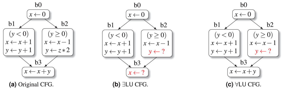
Figure 1: The effect of LU variable propagation on a simple CFG.
We conclude this section by clarifying the soundness relation existing between the results obtained by the target numeric static analysis, computing on the numeric abstract domain A, and the concrete semantics of the program, computing on the concrete domain C. Given an input CFG , the concrete semantics computes a map associating a concrete invariant to each node of G. Let be the map of abstract invariants for G computed using abstract domain A; then, since the numeric static analysis is known to be sound, for each node we have
For an arbitrary LU variables map , let be the CFG produced by Algorithm 1 when applied to G and . Notice that the algorithm only modifies the contents of the basic blocks of G, without changing its structure; hence, we can easily associate each node to the corresponding node . Let be the map of abstract invariants for G′ computed using abstract domain A; then, for each node , letting be the corresponding node in G′, we obtain
meaning that the program transformation is sound when applied to a numeric static analysis no matter the accuracy of the oracle used.
Note that, in general, the stronger result does not necessarily hold; this is due to the potential application of non-monotonic abstract semantics operators (e.g., widening). It is also worth stressing that a program transformation such as the one used in Algorithm 1 is sound if the target static analysis is meant to compute an over-approximation of the values of program variables; the transformation may be unsound in more general contexts, e.g., a liveness analysis (Cousot, 2019b).
Implementation and experimental evaluation
The ideas presented in the previous section have been implemented and experimentally evaluated by adapting the open source static analysis tool Clam/Crab (Gurfinkel & Navas, 2021). In the Crab program representation (CrabIR), a nondeterministic assignment to a program variable var is encoded by the abstract statement havoc(var): the variable is said to be havocked by the execution of this statement. By adopting the Crab terminology, we will call havoc analyses the heuristic pre-analyses detecting LU variables, described in ‘A Dataflow Analysis for LU Variables’; similarly, we will call havoc transformation the program transformation described in ‘The Program Transformation Step’; and we will call havoc processing the combination of these two computational steps. In contrast, we will call target analysis the static analysis phase collecting the invariants that are of interest for the end-user.
The static analysis pipeline
We now describe the steps of the overall analysis process, which are summarized in Fig. 2. In the figure, the processing steps are label from Step A to Step H; for each processing step, a directed edge connects its input to its output; blue edges correspond to the processing steps of the original analysis pipeline; red edges highlight the steps that differentiate the modified analysis pipeline from the original one; gray edges, which do not really belong to the static analysis pipeline, correspond to those processing steps that have been added to compare the precision of the target analysis and to assess the accuracy of the LU oracles.
-
Step A
The input program under analysis is parsed by Clang/LLVM, producing the corresponding LLVM bitcode representation which is then fed as input to clam-pp, the Clam preprocessor component. By default, clam-pp applies a few program transformations, such as the lowering of switch statements into chains of conditional branches; more importantly, in our experiments we systematically enabled the inlining of known function calls, so as to improve the call context sensitivity of the analysis when performing an intra-procedural analysis. Note that Clam/Crab also supports inter-procedural analyses: these are typically faster than full inlining, but quite often produce less precise results.
-
Step B
The Clam component translates the LLVM bitcode representation into CrabIR, which is an intermediate representation specifically designed for static analysis. In this translation phase a few program constructs that the analysis is unable to model correctly and precisely, e.g., calls to unknown external functions, are replaced by (sequences of) havoc statements. This phase also removes all LLVM phi-instructions, which implement the -nodes of the SSA form, replacing them with additional basic blocks containing assignment statements.
-
Step C
The havoc analysis computes the set of program variables that are likely unconstrained at the exit of each basic block of the CrabIR representation. As discussed in ‘Detecting Likely Unconstrained Variables’, this step is not subject to a strict safety requirement and hence, in principle, its implementation could be based on any reasonable heuristics; we model it as a classical static analysis and we implemented it by using the Crab component itself.
-
Step D
This step performs the havoc transformation, using the results of the analysis of Step C to rewrite the CrabIR representation produced by Step B; this is implemented as a simple visitor of the CrabIR CFG, corresponding to Algorithm 1, replacing assignment statements with havoc statements.
-
Step E
The final processing step is the target static analysis, which reuses the Crab component to compute an over-approximation of the semantics of the havocked CrabIR representation produced by Step D, using the target abstract domain chosen at configuration time. The invariants computed are stored and made available to the post-analysis processing phases (assertion checks, program annotations, etc.).
-
Step F
In contrast, when the havoc analysis is disabled (i.e., when the analysis toolchain is used without modification), the target static analysis is computed as described in Step E above, but starting from the original CrabIR representation produced by Step B.
-
Step G
The target-analysis loop invariants produced in Step E and Step F are systematically compared for precision using the clam-diff tool.
-
Steps H1/H2
The havoc analysis and transformation steps are checked for accuracy by comparing the havoc invariants produced in Step C with the ground truth target-analysis invariants produced in Step F; the details of this accuracy assessment are described in ‘Assessing the Accuracy of LU Oracles’.
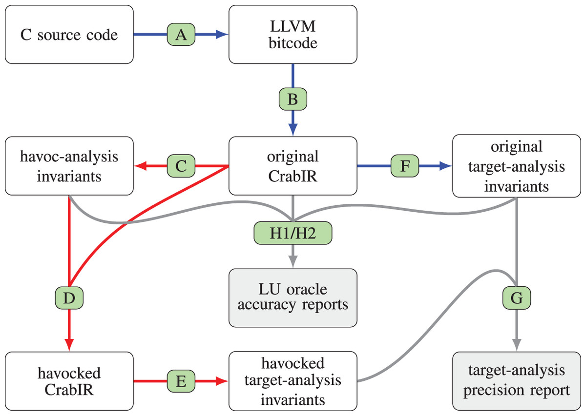
Figure 2: Processing steps of the Clam/Crab toolchain, also including the precision comparison.
(A) Clang/LLVM+clam-pp; (B) Clam; (C) havoc-analysis; (D) havoc-propagation; (E/F) target-analysis; (G) clam-diff; (H1/H2) ad-hoc code.
As target analyses we will consider the classical numerical analyses based on the abstract domain of intervals (Cousot & Cousot, 1977), for the non-relational case, and the abstract domain of convex polyhedra (Cousot & Halbwachs, 1978), for the relational case. Namely, for the domain of intervals we adopt the implementation that is built-in in Crab, whereas for the domain of convex polyhedra we opt for the implementation provided by the PPLite library (Becchi & Zaffanella, 2018a, 2018b, 2020), which is accessible in Crab via the generic Apron interface (Jeannet & Miné, 2009). Note that we are considering the Cartesian factored variant (Halbwachs, Merchat & Gonnord, 2006; Singh, Püschel & Vechev, 2017) of this domain, which greatly improves the efficiency of the classical polyhedral analysis by dynamically computing optimal variable packs, thereby incurring no precision loss. A recent experimental evaluation (Arceri, Dolcetti & Zaffanella, 2023a) has shown that the PPLite’s implementation of this domain is competitive with the one provided by ELINA (Singh, Püschel & Vechev, 2017), which is considered state-of-the-art.
The experiments described in the article have been run on a few machines, using different operating systems; the experiments meant to evaluate efficiency have been run on a ‘MacBookPro18,3’, with an Apple M1 Pro CPU and 16 GB of RAM; in our configuration the analysis pipeline is sequential, making no use of multi-threading and/or process-level parallelism.
The benchmarks for the experimental evaluation
The preliminary experimental evaluation conducted in Arceri, Dolcetti & Zaffanella (2023b), using the first prototype of the havoc analysis and transformation steps, initially considered the C source files distributed with PAGAI (Henry, Monniaux & Moy, 2012), which are variants of tests taken from the SNU real-time benchmark suite for WCET (worst-case execution time) analysis. Most of these benchmarks are synthetic ones: they were probably meant to assess the robustness of a WCET analysis tool when handling a variety of control flow constructs. Hence, the experimental evaluation in Arceri, Dolcetti & Zaffanella (2023b) extended the set of tests by also considering 10 Linux drivers from the SV-COMP repository (https://github.com/sosy-lab/sv-benchmarks/tree/master/c/ldv-linux-4.2-rc1): being (minor variants of) real code, these benchmarks are typically larger and arguably more interesting than the synthetic ones. For this reason, here we avoid repeating the experimental evaluation for the PAGAI benchmarks, referring the interested reader to Arceri, Dolcetti & Zaffanella (2023b); rather, we extend the set of the more meaningful benchmarks by considering a larger number of Linux drivers. The reader is warned that, since the improved havoc analysis and transformation steps are not fully equivalent to the initial prototype of Arceri, Dolcetti & Zaffanella (2023b), little variations with respect to the experimental results shown in Arceri, Dolcetti & Zaffanella (2023b) should be expected.
In Table 12 (shown in the Appendix) we provide a few metrics for each Linux driver, whose source code is stored in a single file and hence gets translated into a single LLVM bitcode module. The first column associates a unique identifier (‘d ’) to each of the 30 Linux drivers, whose shortened names are shown in the second column; the next eight columns provide the values for the considered metrics. For convenience, the detailed information in Table 12 is summarized in Table 1: namely, for each of the eight columns of Table 12, we report in the rows for Table 1 its arithmetic mean and standard deviation, as well as the most commonly used percentiles (minimum value, first quartile, median, third quartile and maximum value)3 . The reader is warned that, from now on, we will refer to this kind of statistics for what they are, i.e., descriptive statistics for the considered set of benchmarks; no generalization or extrapolation to different contexts is meant.
| Without inlining | With inlining | |||||||
|---|---|---|---|---|---|---|---|---|
| Fun | Var | Node | Stmt | Fun | Var | Node | Stmt | |
| Mean | 264.1 | 2,528.9 | 2,728.0 | 4,596.4 | 15.5 | 7,196.5 | 1,4948.5 | 19,813.6 |
| Std dev | 129.7 | 2,196.0 | 1,701.0 | 3,278.3 | 14.8 | 6,984.1 | 14,708.9 | 22,766.3 |
| Min value | 86 | 332 | 457 | 659 | 1 | 58 | 208 | 177 |
| 1st quartile | 150 | 1,063 | 1,511 | 2,262 | 4 | 2,135 | 3,899 | 5,250 |
| Median | 238 | 1,979 | 2,481 | 4,117 | 10 | 5,610 | 10,971 | 13,030 |
| 3rd quartile | 382 | 2,719 | 3,382 | 5,181 | 27 | 8,036 | 19,608 | 22,532 |
| Max value | 494 | 10,747 | 8,078 | 13,554 | 49 | 24,957 | 62,327 | 108,630 |
The four rightmost columns of Table 1 show the number of functions (‘fun’), numeric variables (‘var’), CFG basic blocks (‘node’) and elementary statements (‘stmt’) of the “original CrabIR representation”, as obtained after Step B of the Clam/Crab pipeline. In the CrabIR representation, the elementary statements (‘stmt’) do not include the basic block terminators, i.e., those statements such as ‘goto’ and ‘return’ encoding the edges of the CFG of each function; hence, it may happen that a CFG has more nodes than statements. More importantly, since our LU oracles are only targeting numeric information, when counting program variables (‘var’) we only considered those having a numeric datatype, i.e., those that in the CrabIR representation have a scalar integer or real type; hence, we disregard Boolean variables, aggregate type variables (i.e., arrays) and references to memory regions (i.e., pointers). As a matter of fact, floating point variables are ignored too, because the Crab static analyzer does not fully support this datatype; as a result, even though in principle nothing would prevent our transformation to be applied to floating point variables, in the considered experimental setting it only targets integer ones.
As already noted, this program representation is the result of several transformations, including the LLVM function inlining pass computed in Step A. To better highlight the practical impact of this pass, on the left of the rightmost four columns described above we show the results that would have been obtained, for the same set of metrics, when disabling the function inlining step (i.e., when invoking the tool clam.py without passing option ––inline). Clearly, this program transformation deeply affects both the precision and the efficiency of any numeric analysis: on the one hand, function inlining tends to generate bigger functions, having more basic blocks and variables and hence allowing for the propagation of more contextual information; on the other hand, the same transformation allows for removing the code of all the (already inlined) auxiliary functions having internal linkage, which do not need to be analyzed in isolation.
The impact on code of the havoc transformation
Table 2 summarizes, by means of the usual descriptive statistics, the effects on the CrabIR representation of the 4 havoc transformation variants; the details for each driver can be found in Table 13 in the Appendix. The second column of the table (‘check’) reports on the number of checks performed during the havocking process, i.e., the number of executions of the conditional test in line 4 of Algorithm 1. This number, corresponding to the maximum number of statements that could potentially be havocked, is smaller than the overall number of statements of each driver (reported in the last column of Table 1), because as said before the havoc transformation pass only considers the assignment-like statements that operate on variables having a numeric datatype. The following four columns reports on the percentage of assignment-like statements that are actually havocked when adopting each variant of the havoc analysis, i.e., the percentage of executions where the test in line 4 of Algorithm 1 is satisfied.
| % Statements havocked | |||||
|---|---|---|---|---|---|
| Check | |||||
| Mean | 7,140.0 | 57.79 | 51.89 | 15.23 | 14.61 |
| Std dev | 16,619.8 | 22.20 | 21.81 | 16.07 | 15.86 |
| Min value | 15 | 5.67 | 5.57 | 0.00 | 0.00 |
| 1st quartile | 1,285 | 43.87 | 36.08 | 4.80 | 4.80 |
| Median | 3,299 | 59.09 | 54.49 | 9.23 | 9.19 |
| 3rd quartile | 5,533 | 73.87 | 69.45 | 22.57 | 20.42 |
| Max value | 92,146 | 97.23 | 84.76 | 79.10 | 79.09 |
When looking at the data as summarized in Table 2 we observe that the overall effect of the havoc transformation varies significantly depending on the oracle variant chosen. When comparing the percentages of statements havocked by the four oracle variants, going from left to right, we see that the oracle variants become more and more conservative, confirming the intuitive expectations:
-
the relational oracles are more conservative than the non-relational ones;
the universal oracles are more conservative than the existential ones;
the choice between non-relational and relational oracles has a much greater impact than the choice between existential and universal variants.
Roughly speaking, on the considered benchmarks the transformations based on the relational variants seem really conservative; in contrast, the non-relational ones look rather aggressive, potentially leading to much more significant effects on the precision and efficiency of the target analysis. Observing the percentile values it can be seen that the effect of the havoc transformation step also varies significantly depending on the considered test. By looking at the detailed data in Table 13, we see that almost all tests are affected by the havoc transformation, the only exceptions being drivers ‘d03’ and ‘d14’ when considering the relational oracles: these two drivers are among those having the smallest number of havoc checks (i.e., havocable statements); also, even for these small tests the non-relational oracles are able to havoc a significant fraction of the statements.
The percentage of havocked statements4 computed on all tests (see the last line in Table 13) is 78.32% for the non-relational oracle , while being 10.52% for the relational oracle ; the percentages for the corresponding universal oracles and are slightly smaller (69.04% and 10.07%, respectively).
Regarding efficiency (i.e., the computation overhead caused by the havoc processing step in the overall static analysis pipeline), in Table 13 we report, for each driver and each oracle variant, the time spent in the havoc processing steps (Step C and Step D of Fig. 2). We observe that for most of the drivers the time consumed by these processing steps is reasonably small, with a few notable exceptions: in particular, the time spent in the havocking process for ‘d01’ is greater than the time spent on all the other 29 drivers. It should be stressed that most of the processing time is spent in the havoc analysis phase (Step C); only a tiny fraction of the havoc processing time is spent on the havoc transformation phase (Step D). We note in passing that the havoc analysis based on the universal LU oracles happens to be slower. This has to be expected, by the following reasoning:
-
the efficiency of the havoc analysis is (negatively) correlated with the size of the sets of variables that need to be propagated;
hence, to improve efficiency, at the implementation level the havoc analysis represents and propagates the complement of the set of LU variables (i.e., the set of constrained variables), because it is typically much smaller than ;
the universal oracles, being more conservative than the relational ones, compute smaller sets, which ends up computing and propagating larger set complements.
Assessing the accuracy of lu oracles
In this section we provide an assessment of the accuracy of our LU oracles, i.e., their ability to correctly classify program variables as constrained or unconstrained with respect to a static analysis. This assessment is useful because, as explained before, our LU oracles are only meant to heuristically guess which variables are unconstrained: in principle, one could replace them by different oracles, possibly based on alternative implementation techniques (e.g., adopting a machine learning approach), so as to try and obtain a better precision/efficiency trade-off in the target analysis. Our assessment is thus meant to highlight the code patterns where precision could be improved and, maybe more importantly, those patterns where it cannot be improved, so as to better focus any further implementation effort.
We will first consider a qualitative assessment, by providing simple examples where the LU oracle classification fails; then we will focus on a quantitative assessment, measuring how often these classification failures occur in our benchmark suite.
Qualitative accuracy assessment
As briefly mentioned before, our LU oracles are not based on Abstract Interpretation theory and, in particular, the semantic transfer functions sketched in ‘Detecting Likely Unconstrained Variables’ are not meant to be formally correct: as a result, when classifying the program variables as constrained or unconstrained, they are subject to both false positives and false negatives.
For ease of exposition, in the following we will mainly refer to the existential variant of the non-relational LU oracle ( ), matched by the corresponding target analysis using the domain of intervals; the reasoning is easily adapted to apply to the other variants.
As discussed before, for each program point , the LU oracle computes the set of likely unconstrained variables, thereby predicting numeric variable to be unconstrained when . The results of the target numerical static analysis using the domain of intervals (on the unmodified program) is used as ground truth: variable is unconstrained at program point if the invariant computed at states that ; variable is constrained at program point if the computed invariant at states that , where at least one of and is a finite bound; as a special case, when the target analysis computes the bottom element , i.e., when it flags the program point as unreachable code, then all variables in are constrained in . Therefore, these are the possible outcomes of the LU variable classification phase:
True Positive (TP): the oracle predicted and the target analysis is computing a program invariant where is indeed unconstrained;
True Negative (TN): the oracle predicted and the target analysis is computing an invariant where is indeed constrained;
False Positive (FP): the oracle predicted but the target analysis is computing an invariant where is constrained;
False Negative (FN): the oracle predicted but the target analysis is computing an invariant where is unconstrained.
A too aggressive LU oracle, characterized by a high percentage of FP, will likely cause more precision losses in the target numerical analysis, possibly improving its efficiency; in contrast, a too conservative LU oracle, characterized by a high percentage of FN, will preserve the precision of the target analysis, while also having a limited impact on its efficiency.
In Fig. 3 we provide examples of C-like code witnessing that all the classification outcomes are indeed possible when using the non-relational LU oracles. In these examples, all variables are of integer type and a nondeterministic assignment such as ‘ ’ is simulated by x = nondet(), where the function call in the right-hand side returns each time an arbitrary integer value. Note that the comments are not meant to show the complete invariant computed when using the interval domain; rather, we only show the portion of the invariant which is relevant to compute the interval value for variable at the end of each chunk of code.
Figure 3: Examples of classification outcomes.
The examples of TP and TN shown in Figs. 3A and 3B need no explanation and are only provided for the sake of completeness.
False Positives. The FP example in Fig. 3C is rather involved and deserves an explanation. In principle, a FP could be obtained more easily by processing the simpler code in Fig. 3D: here, since in line 5 we have , the transfer function of Eq. (4) will also flag as LU, while the interval analysis is able to detect a multiplication by zero and hence conclude that is actually constrained. However, this simple code pattern cannot be observed in the context of our experimental evaluation because, during Step A of the Clam/Crab toolchain, the last assignment x = y * z is automatically simplified to the constant assignment x = 0: the simplification is triggered by the InstCombine LLVM bitcode transform pass (https://llvm.org/docs/Passes.html#instcombine-combine-redundant-instructions), which is invoked by the Clam preprocessor clam-pp. To avoid this, lines 1–6 of Fig. 3C implement a “mildly obfuscated” assignment of the constant value 0 to variable : on the one hand, the code is complicated enough to confuse the InstCombine transformation step; on the other hand, the code is simple enough to be precisely modeled by the static analysis using the domain of intervals.
The observation above has significant consequences from a practical point of view: since the code we are analyzing is the result of some program transformation/simplification steps, there are code patterns that will never occur in practice and hence can be simply ignored when defining the transfer functions of our LU oracles, without affecting their accuracy. For instance, we could simplify the transfer function in Eq. (5), by ignoring the special case ; similarly, we could simplify the transfer function in Eq. (4) by ignoring the special case . This is also the reason why our LU oracles, by design, are unable to distinguish between reachable and unreachable code: in principle, one could lift the abstract domain by adding a distinguished bottom element to encode unreachability and then complicate the transfer function of Eq. (5) so as to detect the special cases and , which are triggering definite division by zero errors. However, these cases too are going to be simplified away in Step A of our toolchain and hence they never occur in our experimental evaluation. Clearly, the design choices above should be reconsidered when targeting different static analysis toolchains that do not apply the above mentioned program transformation/simplification steps.
In Fig. 3E we can see another example of FP, but having a different root cause: intuitively, the static analysis using the domain of intervals can sometimes flag an execution path as unreachable, whereas this precision level cannot be achieved by the LU oracle. In lines 1–4 of Fig. 3E we see again the code pattern to obtain an obfuscated assignment of value zero to variable ; knowing that , the interval analysis can flag the else branch in lines 8–10 as unreachable code, whereas this code is reachable for the LU oracle. Hence, we obtain a FP for at line 10, where the oracle would predict ; this FP is also propagated to line 11 where, by merging the invariants computed in the two branches of the if-then-else construct, the oracle will still predict , even though is actually constrained. Note that, in this example, the universal variant of our oracle would correctly flag as constrained at line 11: however, this is only happening by chance; in general, the oracle is more prone at generating a FN.
False Negatives. The code in Fig. 3F shows an example of FN: when reaching line 7, we have both and so that, by following Eq. (4), our LU oracle will conclude that is constrained at line 8; however, this is not the case because in the interval domain we obtain . The code in Fig. 3G shows that another FN can be similarly obtained due to control flow. Here, variable is unconstrained on line 2; then, the abstract evaluation of the conditional guard (x >= 0) on line 3 leads to using twice Eq. (7) to process predicates and , so that becomes constrained in both branches of the if-then-else statement (lines 4 and 7); when later merging the invariants of the two computational branches, the oracle will still report as constrained (i.e., on line 9), but this is not the case because in the interval domain we obtain .
These two FN examples could be avoided by modifying our LU oracles to track more information5 . Namely, the oracle could track separately the constrainedness of the lower and upper interval bounds, so as to distinguish for each variable the four cases: (i.e., has both a lower and an upper bound); (i.e., has only the lower bound); (i.e., has only the upper bound); and (i.e., is unconstrained). While interesting, such an approach seems to be tailored to the case of the non-relational LU oracles; we also conjecture that, in general, it would result in a limited gain of precision, while somehow complicating the definition of the transfer functions of the LU oracle.
The code in Fig. 3H shows another example of FN which is caused by the use of the widening operator on the interval domain. When entering the loop on line 3, variable has value zero, so that ; in the loop body, variable is nondeterministically incremented or decremented, so that it remains constrained; hence, the LU oracle quickly converges to a fixpoint where . In contrast, when using the interval domain, the loop is entered knowing that and each iteration of the loop body will ideally compute a new interval along the infinite ascending chain
To avoid nontermination, the static analysis tool will resort to the use of the interval widening operator, thereby reaching the loop fixpoint invariant after computing
Hence we obtain a FN, because the oracle predicts whereas the target analysis actually computes ; this loop invariant is propagated to line 9.
This example of a FN that is caused by the use of widenings in the target analysis is quite interesting. Roughly speaking, such a loss of accuracy of the LU oracle is to be expected because widenings were not taken into account when defining its transfer functions. In principle, by also considering widenings, a modified LU oracle could more faithfully mimic the actual static analysis computation by also guessing when the use of widening operators would eventually cause a constrained variable to become unconstrained. This approach could be interpreted as some sort of dual of loop acceleration (Gonnord & Schrammel, 2014): the goal of loop acceleration techniques, which target loop constructs satisfying some specific properties, is to enhance precision by computing the exact abstract fixpoint of the loop via some algebraic manipulation of the loop body transfer function; hence, Kleene iteration is avoided and, in particular, the precision losses caused by widenings are avoided. Reasoning dually, a new LU oracle could be designed to identify those loops where a huge precision loss is likely to occur, possibly due to the use of widenings: hence, even in this case Kleene iteration would be avoided, but this time with the goal of accelerating the unavoidable precision losses. The main problem with such an approach is that the effects of widening operators are far from being easily predictable. To start with, these operators are typically non-monotonic (Cousot & Cousot, 1977). Moreover, since by definition widenings are not meant to satisfy a best precision requirement, an abstract domain may be provided with several, different widening operators: for instance, in their implementations of the domain of convex polyhedra, libraries PPL (Bagnara, Hill & Zaffanella, 2008) and PPLite (Becchi & Zaffanella, 2020) provide both the standard widening of Halbwachs (1979) and the improved widening operator proposed in Bagnara et al. (2003). On top of this, widening operators are often combined with auxiliary techniques that are meant to throttle their precision/efficiency trade-off: an incomplete list includes the use of descending iterations with narrowing (Cousot & Cousot, 1977), delayed widening (Cousot & Cousot, 1992), widening up-to (Halbwachs, Proy & Raymond, 1994), widening with thresholds (Blanchet et al., 2003), lookahead widening (Gopan & Reps, 2006) and intertwining widening and narrowing (Amato et al., 2016). The choice of a specific combination of techniques is typically left to the configuration phase of the static analysis tool: as an example, the fixpoint approximation engine implemented in Clam/Crab intertwines widening and narrowing, also delaying the application of widenings for a few iterations; widening thresholds are also supported, but these were not used in our experimental evaluation. To summarize, any prediction of the effects of widenings is bound to be strongly coupled with the specific widening implementation and configuration adopted in the considered static analysis tool.
Quantitative accuracy assessment for havoc analysis
Having discussed the potential sources of false positives and false negatives from a qualitative point of view, we now focus on a quantitative assessment. We start by checking the accuracy of havoc analysis in isolation, i.e., the accuracy of the invariants produced by the LU oracles independently from their actual use in the havoc transformation phase.
With reference to the Clam/Crab pipeline shown in Fig. 2, in Step H1 we compare the original target analysis invariants produced by Step F (corresponding to the ground truth) with the havoc-analysis invariants produced by Step C. In particular, in the comparison we will use as ground truth the invariants of the interval domain for the non-relational LU oracles, while for the relational LU oracles will be using as ground truth the invariants of the polyhedra domain.
The systematic comparison is implemented by ad-hoc code that we added to the clam executable: for each function in the considered test, we first compute the corresponding set of numeric program variables; then, for each basic block in the CFG of the function, the set of unconstrained variables (ground truth) is extracted by the target analysis invariants computed at the end of ; similarly, the set of LU variables (prediction) is extracted from the havoc-analysis invariants. By comparing these sets, the numbers of TP, TN, FP, FN for basic block are computed and added to corresponding global counters for the considered test.
The detailed results are shown in the Appendix, in Tables 14 and 15; the corresponding descriptive statistics are shown in Tables 3 and 4. With reference to Table 14, the second column (‘check’) reports the total number of oracle predictions that have been checked for accuracy: this number is high because, as said before, it has been obtained by adding, for each function analyzed in the considered driver, the product of the number of numeric variables of the function by the number of its CFG nodes; as an example, since driver ‘d06’ has a single function after inlining, we can directly use the numbers ‘var’ and ‘node’ from Table 12 to compute
| vs intervals | vs intervals | ||||||||
|---|---|---|---|---|---|---|---|---|---|
| Check | TP | TN | FP | FN | TP | TN | FP | FN | |
| Mean | 151.8 M | 97.14 | 0.75 | 2.07 | 0.04 | 58.92 | 1.32 | 1.50 | 38.26 |
| Std dev | 280.1 M | 6.80 | 1.14 | 6.90 | 0.05 | 14.05 | 2.32 | 6.12 | 14.00 |
| Min value | 12.1 K | 64.21 | 0.03 | 0.00 | 0.00 | 12.82 | 0.05 | 0.00 | 3.62 |
| 1st quartile | 3.8 M | 98.54 | 0.11 | 0.03 | 0.01 | 54.32 | 0.23 | 0.07 | 32.02 |
| Median | 25.3 M | 99.31 | 0.41 | 0.13 | 0.02 | 61.34 | 0.54 | 0.16 | 36.05 |
| 3rd quartile | 107.9 M | 99.54 | 0.65 | 0.31 | 0.04 | 66.68 | 1.15 | 0.36 | 44.29 |
| Max value | 1,012.9 M | 99.94 | 4.84 | 35.76 | 0.18 | 83.32 | 12.22 | 33.74 | 73.08 |
| vs polyhedra | vs polyhedra | ||||||||
|---|---|---|---|---|---|---|---|---|---|
| Check | TP | TN | FP | FN | TP | TN | FP | FN | |
| Mean | 151.8 M | 96.58 | 1.00 | 2.11 | 0.30 | 43.09 | 1.67 | 1.44 | 53.80 |
| Std dev | 280.1 M | 6.70 | 1.41 | 6.89 | 0.41 | 15.04 | 2.43 | 5.99 | 16.32 |
| Min value | 12.1 K | 64.20 | 0.03 | 0.00 | 0.00 | 12.11 | 0.07 | 0.00 | 4.83 |
| 1st quartile | 3.8 M | 96.53 | 0.16 | 0.04 | 0.04 | 33.35 | 0.38 | 0.10 | 46.04 |
| median | 25.3 M | 98.75 | 0.53 | 0.20 | 0.11 | 41.37 | 0.74 | 0.15 | 56.30 |
| 3rd quartile | 107.9 M | 99.06 | 0.79 | 0.32 | 0.48 | 53.36 | 2.30 | 0.34 | 64.58 |
| Max value | 1,012.9 M | 99.92 | 5.45 | 35.76 | 1.78 | 81.21 | 12.39 | 33.06 | 79.31 |
The next four columns of Table 14 show the percentages of TP, TN, FP and FN obtained when using the existential oracle ; these are followed by another set of four columns, for the universal oracle .
The descriptive statistics in Table 3 show us that for oracle the average percentages of FP and FN are as low as 2.07% and 0.04%, respectively. While interesting, these descriptive statistics are not the most adequate ones for our accuracy assessment. Hence, in Table 5 we show the values obtained for the metrics commonly used for binary classifiers6 :
‘accuracy’, computed as
‘recall’, computed as
‘precision’, computed as
‘FPR’ (FP rate), computed as
‘FNR’ (FN rate), computed as
‘F1’ (balanced F-score), computed as
| Oracle | Accuracy | Recall | Precision | FPR | FNR | F1 |
|---|---|---|---|---|---|---|
| 0.9667 | 0.9998 | 0.9669 | 0.9734 | 0.0002 | 0.9831 | |
| 0.6821 | 0.6971 | 0.9669 | 0.7423 | 0.3029 | 0.8101 | |
| 0.9649 | 0.9980 | 0.9667 | 0.9619 | 0.0020 | 0.9821 | |
| 0.5505 | 0.5584 | 0.9667 | 0.6704 | 0.4416 | 0.7079 |
It can be seen that the existential oracles are characterized by rather good values for all the metrics, with the exception of ‘FPR’, which is really high. When moving to the universal oracles, ‘precision’ is almost unaffected but we observe a significant decrease of ‘accuracy’ and ‘recall’ values, with a consequential effect on ‘F1’. These are the direct consequences of the increase in the number of FN, which is expected for what we said in our qualitative assessment. Note that the ‘F1’ score, being balanced, is giving equal importance to FP and FN misclassifications: in our context, a conservative oracle should prefer a FN (i.e., missing an opportunity to improve the efficiency of the target analysis) to a FP (i.e., potentially incurring a precision loss in the target analysis); an aggressive oracle would rather prefer the other way round. Hence, depending on context, one may opt for using the Fβ score
so as to weight more TP or TN depending on the value of .
In order to explain the high value of ‘FPR’, we performed a further investigation focusing on those few tests having a high percentage of FP: this allowed us to conclude that these high percentages are directly caused by those program points that are detected to be unreachable by the target-analysis (e.g., the interval analysis in the non-relational case, as is the case for lines 8–10 in Fig. 3E). Looking at the details in Table 14, we see that FP values above 10% are only recorded for drivers ‘d09’ (35.76%) and ‘d21’ (13.97%). As an example, the CFG for function ‘main’ in driver ‘d09’ has 11,967 nodes and 19,338 numeric variables; the interval invariant is computed on 4,281 nodes, leading to checks where the ground truth declares the variable to be constrained due to the unreachability of the node. Since the LU oracle is unable to flag these nodes as unreachable, it classifies almost all of these variables as unconstrained, thereby recording 82,742,672 FP (99.5%) and only 43,306 TN (0.05%). If these unreachable nodes were ignored, for the whole driver we would obtain 1,076 FP, so that the FP percentage would drop from 35.76% to less than 0.01%.
Roughly speaking, the quantitative assessment for the havoc analysis is somehow questionable: by checking the prediction of each variable in each basic block, a correct/wrong prediction is recorded even for those variables that never occur in the considered basic block, adding significant noise to the accuracy assessment. For this reason, in the following section we complement our accuracy assessment for the LU oracles by focusing on the predictions that come into play in the havoc transformation phase.
Quantitative accuracy assessment for havoc transformation
As said above, we now turn our attention to the oracle predictionsa that are actually used during the havoc transformation phase. With reference to the Clam/Crab pipeline shown in Fig. 2, in Step H2 we still compare the original target analysis invariants produced by Step F with the havoc-analysis invariants produced by Step C, but now we also take into account the transformation working on the ‘original CrabIR’; namely, we will only check the accuracy of the LU oracle predictions (with respect to the ground truth provided by the target analysis) when executing the conditional test in line 4 of Algorithm 1.
The detailed results of this accuracy assessment are shown in the Appendix in Tables 16 and 17, which have the same structure of Tables 14 and 15 discussed in the previous section; the main difference is that now the contents of the second column (‘check’) correspond to the number of havoc tests computed during the execution of Algorithm 1 (which is the same number already reported in Table 13).
As before, in Tables 6 and 7 we provide the usual descriptive statistics for Tables 16 and 17, respectively; also, the binary classification metrics are shown in Table 8. Here we can see that for the ‘accuracy’ and ‘precision’ metrics we obtain values as good as the ones in Table 5; we record lower values for ‘recall’, as a direct consequence of the increase in the percentage of FN (less evident for the oracle). As expected, significantly better values are obtained for the ‘FPR’ metrics, specially for the relational oracles; as discussed in the previous section, this is mainly due to the reduced fraction of FP generated by the unreachable CFG nodes. Interestingly, when comparing to Table 5, ‘FNR’ values are significantly increasing for existential oracles and decreasing for universal ones (with corresponding effects on ‘F1’): in other words, the effects of FN misclassifications are mitigated when focusing on the actual use of the havoc analysis results.
| vs intervals | vs intervals | ||||||||
|---|---|---|---|---|---|---|---|---|---|
| Check | TP | TN | FP | FN | TP | TN | FP | FN | |
| Mean | 7,140.0 | 56.93 | 37.88 | 0.86 | 4.33 | 51.05 | 37.89 | 0.84 | 10.22 |
| Std dev | 16,619.8 | 22.55 | 19.74 | 3.50 | 9.13 | 21.96 | 19.75 | 3.50 | 9.83 |
| Min value | 15 | 5.67 | 2.75 | 0.00 | 0.00 | 5.57 | 2.75 | 0.00 | 0.00 |
| 1st quartile | 1,285 | 41.26 | 21.98 | 0.00 | 0.21 | 35.19 | 21.98 | 0.00 | 4.32 |
| Median | 3,299 | 59.01 | 34.33 | 0.01 | 1.66 | 53.77 | 34.33 | 0.00 | 8.45 |
| 3rd quartile | 5,533 | 71.77 | 50.14 | 0.15 | 2.93 | 68.93 | 50.14 | 0.13 | 13.56 |
| Max value | 92,146 | 97.23 | 86.38 | 19.12 | 44.70 | 84.35 | 86.38 | 19.12 | 44.79 |
| vs polyhedra | vs polyhedra | ||||||||
|---|---|---|---|---|---|---|---|---|---|
| Check | TP | TN | FP | FN | TP | TN | FP | FN | |
| Mean | 7,140.0 | 14.73 | 81.56 | 0.51 | 3.21 | 14.11 | 81.56 | 0.50 | 3.83 |
| Std dev | 16,619.8 | 16.05 | 16.67 | 0.76 | 3.10 | 15.83 | 16.67 | 0.76 | 3.55 |
| Min value | 15 | 0.00 | 20.86 | 0.00 | 0.00 | 0.00 | 20.86 | 0.00 | 0.00 |
| 1st quartile | 1,285 | 4.80 | 74.69 | 0.00 | 0.59 | 4.77 | 74.69 | 0.00 | 0.71 |
| Median | 3,299 | 9.07 | 86.42 | 0.11 | 2.41 | 9.03 | 86.42 | 0.11 | 3.13 |
| 3rd quartile | 5,533 | 21.56 | 91.44 | 0.89 | 4.57 | 19.62 | 91.44 | 0.89 | 5.75 |
| Max value | 92,146 | 79.07 | 100.00 | 3.26 | 10.77 | 79.06 | 100.00 | 3.26 | 12.23 |
| Oracle | Accuracy | Recall | Precision | FPR | FNR | F1 |
|---|---|---|---|---|---|---|
| 0.9560 | 0.9580 | 0.9871 | 0.0524 | 0.0420 | 0.9723 | |
| 0.8633 | 0.8430 | 0.9871 | 0.0521 | 0.1570 | 0.9094 | |
| 0.9769 | 0.8353 | 0.9716 | 0.0034 | 0.1647 | 0.8983 | |
| 0.9724 | 0.7988 | 0.9716 | 0.0034 | 0.2012 | 0.8768 |
In summary, this accuracy assessment seems to confirm most of the observations we made in ‘The Impact on Code of the Havoc Transformation’ when discussing Table 2, somehow providing an explanation for them:
-
the relational oracles, having significantly lower ‘FPR’ and ‘recall’, happen to be more conservative than the non-relational ones;
the universal oracles, having lower ‘recall’, are more conservative than the existential ones.
Precision and efficiency of the target analyses
Having discussed at length the accuracy of the four variants of havoc analysis and transformation in the previous section, we now move to the final part of our experimental evaluation, whose goal is to measure the effectiveness of the havoc processing steps in affecting the precision/efficiency trade-off of the target numerical static analysis.
The effect of havoc transformation on target analysis precision
We start by evaluating how the havoc transformation affects the precision of the target static analysis: with reference to the Clam/Crab toolchain of Fig. 2, in Step G we systematically compare the ‘original target-analysis invariants’, obtained in Step F by analyzing the original CrabIR representation, with the ‘havocked target-analysis invariants’, obtained in Step E by analyzing the havocked CrabIR representation.
We first discuss the results obtained when using the interval domain in the target static analysis. Table 18 in the Appendix shows the detailed results obtained when comparing the original interval analysis (‘intervals’) with the havocked interval analyses using the non-relational oracles (‘ -intervals’ and ‘ -intervals’). In the table, after the test identifier (‘test’), for the original interval analysis we report the number of invariants computed (‘inv’) and the overall size of these invariants when represented as linear constraint systems (‘cs’). Note that we only consider the target invariants computed at widening points7 , i.e., at most one invariant for each loop in the CFG. To compute the size of the constraint systems we use a slightly modified version of the clam-diff tool, where we force a minimized constraint representation so as to (a) avoid redundant constraints and (b) maximize the number of linear equalities; after that, if each invariant has equalities and inequalities, we compute
The next eight columns are divided in two groups, for the ‘ -intervals’ and ‘ -intervals’ analyses. The first two columns (‘eq’ and ‘gt’) of each group report the number of invariants on which the havocked interval analysis computed the same result (‘eq’) and a precision loss (‘gt’) with respect to the original interval analysis; note that the tool clam-diff also provides counters for the case of a precision improvement (‘lt’) and the case of uncomparable precision (‘un’): these have been omitted from our tables because, in all of the experiments, they are always zero8 . The next two columns in each group (‘ cs’ and ‘ cs’) provide a rough quantitative evaluation of the precision losses incurred by the havocked target analysis: column ‘ cs’ reports the size decrease for the computed linear constraint systems; column ‘ cs’ reports the same information in relative terms, as a percentage of ‘cs’.
As usual, the contents of Table 18 are summarized in Table 9 by the corresponding descriptive statistics. For this specific comparison, it suffices to say that the ‘ -intervals’ analysis computes the very same invariants for 27 of the 30 tests, the exceptions being ‘d05’, ‘d25’ and ‘d29’; the ‘ -intervals’ analysis is able to obtain equal precision also for ‘d25’. When a precision loss is recorded, quite often the only difference between the compared invariants is one or two missing linear equalities; hence, the mean values for ‘ cs’ are less than 0.5%.
| intervals | -intervals | -intervals | ||||||||
|---|---|---|---|---|---|---|---|---|---|---|
| inv | cs | eq | gt | cs | cs | eq | gt | cs | cs | |
| Mean | 387.9 | 12,230.8 | 376.6 | 11.3 | 37.4 | 0.41 | 377.4 | 10.5 | 35.8 | 0.33 |
| Std dev | 812.7 | 34,828.8 | 812.8 | 40.6 | 156.0 | 1.63 | 812.5 | 40.6 | 156.2 | 1.57 |
| Min value | 7 | 22 | 7 | 0 | 0 | 0.00 | 7 | 0 | 0 | 0.00 |
| 1st quartile | 56 | 723 | 38 | 0 | 0 | 0.00 | 38 | 0 | 0 | 0.00 |
| Median | 165 | 3,133 | 160 | 0 | 0 | 0.00 | 160 | 0 | 0 | 0.00 |
| 3rd quartile | 368 | 8,388 | 368 | 0 | 0 | 0.00 | 368 | 0 | 0 | 0.00 |
| Max value | 4,440 | 190,809 | 4,440 | 186 | 828 | 8.57 | 4,440 | 186 | 828 | 8.57 |
When considering the polyhedra domain, things get more interesting. To start with, the results obtained when comparing the original polyhedra analysis (‘polyhedra’) with the havocked polyhedra analyses using the relational oracles (‘ -polyhedra’ and ‘ -polyhedra’) show no precision difference at all on the 30 tests; hence, we omit the corresponding tables. This is largely due to the fact that, as we observed in the previous sections, the relational oracles are overly conservative. Since the end goal of our oracle-based program transformations is to obtain significant efficiency improvements and, to this end, some precision loss is an acceptable trade-off, we now consider a target static analysis where the relational polyhedra domain is combined with a havoc processing phase guided by the non-relational oracles (‘ -polyhedra’ and ‘ -polyhedra’).
The detailed results for these comparisons are shown in Table 19 in the Appendix and summarized in Table 10, whose columns have the same meaning of those in Tables 18 and 9. As expected, for these combinations the results are much more varied. Only three tests (‘d03’, ‘d21’ and ‘d30’) obtain the same precision for all invariants: on average, a precision loss is recorded on more than a half of the computed invariants. However, by observing the percentile values computed for ‘ cs’ in Table 10, it can be seen that these precision losses are somehow limited: for instance, the median values are both below 8%. By looking at the last row (‘all’) in Table 19, which reports the values computed on all tests, we can see that the average constraint system size for the ‘polyhedra’ analysis is and the average constraint system size difference for the ‘ -polyhedra’ analysis is , corresponding to a couple of linear equality constraints; the value is slightly better for the ‘ -polyhedra’ analysis.
| Polyhedra | -polyhedra | -polyhedra | ||||||||
|---|---|---|---|---|---|---|---|---|---|---|
| inv | cs | eq | gt | cs | cs | eq | gt | cs | cs | |
| Mean | 387.9 | 14,982.8 | 143.2 | 244.7 | 1,319.0 | 9.50 | 155.7 | 232.2 | 1,148.9 | 8.13 |
| Std dev | 812.7 | 43,541.3 | 197.6 | 649.3 | 3,493.8 | 8.59 | 246.1 | 595.0 | 2,904.5 | 7.55 |
| Min value | 7 | 28 | 0 | 0 | 0 | 0.00 | 0 | 0 | 0 | 0.00 |
| 1st quartile | 56 | 1,145 | 25 | 10 | 39 | 2.08 | 25 | 10 | 30 | 1.93 |
| Median | 165 | 3,492 | 81 | 54 | 197 | 7.58 | 82 | 53 | 146 | 6.11 |
| 3rd quartile | 368 | 9,132 | 177 | 189 | 828 | 14.53 | 182 | 189 | 828 | 11.30 |
| Max value | 4,440 | 238,969 | 970 | 3,470 | 17,968 | 27.74 | 1,290 | 3,150 | 14,670 | 25.75 |
Going beyond the precision comparison summarized in Table 10, an interesting question is whether or not the choice of combining a relational target analysis with a non-relational LU oracle is going to deeply affect the shape of the target invariants that can be computed: roughly speaking, by following the predictions of a non-relational oracle (which is biased towards preserving only the interval constraints) the program transformation could be compromising the ability of the target polyhedra analysis to compute invariants containing non-interval constraints, i.e., those constraints that can only be defined using 2 or more program variables. We have thus classified the constraints computed by the target analyses on the whole benchmark suite9 , distinguishing between interval and non-interval constraints:
for the (baseline) ‘polyhedra’ analysis, 76.15% of the constraints are interval constraints;
for the ‘ -polyhedra’ analysis, 83.12% of the constraints are interval constraints;
for the ‘ -polyhedra’ analysis, 82.32% of the constraints are interval constraints.
While as expected the percentage of interval constraints is increasing, it can be seen that the havocked polyhedra analyses are still able to compute program invariants containing a significant percentage of inherently relational constraints.
The effect of havoc transformation on target analysis efficiency
For evaluating efficiency, we compare the time spent in the static analysis pipeline in order to obtain the (original or havocked) target analysis invariants.
Intervals
Our experiments on the domain of intervals have shown that the havocked analysis pipeline seems unable to trigger significant efficiency improvements: the original analysis is almost always as efficient as (and quite often more efficient than) the havocked ones. This should not come as a surprise, for the following reasons.
The havoc processing step replaces deterministic assignment statements with nondeterministic ones: the abstract execution on the interval domain is very efficient in both cases. Hence, even though many statements are havocked by the aggressive oracles, the efficiency gain remain marginal, unless the havocking process causes a precision loss that is large enough to influence the overall fixpoint computation; but this is not going to happen, because precision is almost never affected.
The native Crab implementation of the domain of intervals is really efficient; among other things, it systematically trims the abstract environment by removing those variables that are unconstrained. This further mitigates any minor efficiency gain that is triggered by the havocking process.
The havoc processing steps introduce a computational overhead; this might be considered negligible for a static analysis using a computationally heavy domain (such as polyhedra), but not for the domain of intervals. Namely, when considering all tests, the time spent by the havoc processing steps for the oracle is 37.23 s, which correspond to of the 231.36 s that are spent in Step F by the original interval analysis. Hence, all efficiency gains are masked by this overhead.
Roughly speaking, in order to obtain a measurable effect on the precision/efficiency trade-off, we have to consider abstract domains that are computationally more expensive.
Convex polyhedra
As already observed when discussing precision, when using the relational domain of polyhedra we need to choose between the relational and the non-relational LU oracles to guide the havoc transformation step.
When adopting the relational oracles and , the havocked analysis pipeline is still unable to trigger efficiency improvements. Once again, this does not come as a surprise, but for rather different reasons. On the polyhedra domain the havocked assignments would likely obtain a meaningful efficiency gain; however, since the relational LU oracles are too conservative, there is too small a percentage of havocked assignments, so that the overall efficiency gain is limited and once again masked by the overhead of the havoc processing steps.
Hence, we move our attention towards the havocked analyses ‘ -polyhedra’ and ‘ -polyhedra’, which combine the relational domain with a non-relational oracle. In other words, assuming that the original polyhedra analysis will incur a too high computational cost, we configure the analysis pipeline to activate the aggressive non-relational oracles, so as to try and improve its precision/efficiency trade-off. In Table 11 we summarize the results of this efficiency comparison; the details for each driver are available in Table 20 in the Appendix.
| Polyhedra | -polyhedra | -polyhedra | |||||
|---|---|---|---|---|---|---|---|
| speed-up | Speed-up | ||||||
| Mean* | 68.30 | 23.77 | 25.01 | 2.24 | 24.16 | 25.95 | 2.16 |
| Std dev | 110.83 | 41.95 | 45.85 | – | 42.15 | 47.47 | – |
| Min value | 0.01 | 0.01 | 0.01 | 0.97 | 0.01 | 0.01 | 0.93 |
| 1st quartile | 4.70 | 1.73 | 1.77 | 1.11 | 1.72 | 1.78 | 1.09 |
| Median | 13.25 | 5.23 | 5.39 | 1.63 | 5.25 | 5.47 | 1.59 |
| 3rd quartile | 67.36 | 23.53 | 23.81 | 4.62 | 24.66 | 25.15 | 4.54 |
| Max value | 390.49 | 196.65 | 220.16 | 31.77 | 196.77 | 228.94 | 23.91 |
Note:
The main efficiency metric would be the time consumed by the clam.py executable: with reference to the Clam/Crab toolchain of Fig. 2, for the original static analysis, this corresponds to the time spent in steps A, B and F; for the havocked static analyses, this corresponds to the time spent in steps A, B, C, D and E. In order to better understand where efficiency is gained/lost, we rather consider the time consumed in the analysis phase proper, so as to factor out the overhead of the common steps A and B (parsing, LLVM-level program transformations, etc.). Thus, for the original analysis we only measure the time spent in the target analysis step, while for the havocked analyses we measure the overall time spent in the havoc processing and the target-analysis steps; we also report the time spent in the havocked target-analysis considered in isolation. The speed-up is computed as .
The experimental data show that, for the ‘ -polyhedra’ analysis, a speed-up is obtained in 90% of the benchmarks, with minor slow-downs recorded for tests ‘d06’, ‘d18’ and ‘d21’. The median value and geometric mean values for speed-up are 1.63 and 2.24, respectively; 25% of the tests obtain a speed-up of at least 4.6 (3rd quartile).
By comparing ‘ -polyhedra’ with ‘ -polyhedra’, we see that the universal LU oracle is obtaining only a marginal efficiency penalty (on average, less than a second per test). This is interesting because, as seen in the previous section, the ‘ -polyhedra’ analysis also obtains marginally better precision results; in other words, depending on the context, the precision/efficiency trade-off can be tuned by switching between the existential and universal non-relational LU oracles; for the considered tests, a default configuration choosing oracle seems reasonable.
The comparison of with confirms that the havoc processing phases, on average, have a limited impact on efficiency. As a consequence, even though the efficiency of the havoc analysis step could be improved, this would not significantly affect the overall efficiency of the havocked polyhedra analyses.
We conclude this analysis of efficiency by observing that our choice of focusing on the time spent in the analysis phases proper does not introduce significant noise to the experimental data: when considering all tests, corresponds to 96.31% of all the time spent by the executable clam.py for the original ‘polyhedra’ pipeline; similar percentages are obtained for when considering ‘ -polyhedra’ and ‘ -polyhedra’ (93.89% and 94.05%, respectively).
Related work
The four variants of LU variable analysis described in ‘A Dataflow Analysis for LU Variables’ and the abstract program transformation outlined in ‘The Program Transformation Step’, as a whole, can be seen as an instance of the Abstract Compilation approach (Hermenegildo, Warren & Debray, 1992; Warren, Hermenegildo & Debray, 1988) to Abstract Interpretation (Cousot & Cousot, 1977). A few examples (Amato & Spoto, 2001; Boucher & Feeley, 1996; Giacobazzi, Debray & Levi, 1995; Wei, Chen & Rompf, 2019) of application of Abstract Compilation have already been briefly recalled in Section 1; other examples have been recently discussed in De Angelis et al. (2022). A notable distinction between the current proposal and most of the approaches in the literature is that we do not require the program transformation to fully preserve the abstract semantics of the program: since our goal is to tune the efficiency/precision trade-off, we explicitly allow for (hopefully limited) precision losses in the transformation step. In our opinion, this is one of the most relevant differences between abstract and concrete (i.e., traditional) compilation. Note that, in principle, our choice of following the Abstract Compilation approach is not really mandatory. Rather than having offline pre-analysis and program transformation steps, one could have implemented online oracles, to be used in a sort of reduced product with the target numerical analysis: this would have allowed for a dynamic interaction between the oracle and the target numeric domain, resulting in even better oracle predictions. Clearly, it would have also increased the computational overhead, with a negative effect on the overall efficiency of the analysis.
Several articles share with the current proposal the idea of using a lightweight abstract domain to improve the precision and/or efficiency of a target analysis. A few of these can be cast as instances of the A2I framework (Cousot, Giacobazzi & Ranzato, 2019): the silhouette abstraction for shape analyses proposed in Li et al. (2017) provides a weak entailment test that can be efficiently used by the target analysis to guide the merging of disjunctive states, so as to avoid precision losses; similarly, the boxed polyhedra approach put forward in Becchi & Zaffanella (2019) implements a weak entailment test that greatly improves the efficiency of redundancy elimination when using an abstract domain based on sets of polyhedra; both can be classified as online meta-abstract interpretations.
As already explained, our pre-analyses cannot be cast as instances of the A2I framework (in particular, as examples of offline meta-abstract interpretations) because they do not guarantee formal correctness, so that they incur both false positives and false negatives; nonetheless, the formal correctness of the target analysis is maintained. This is the main difference between our current proposal and similar approaches that, in contrast, are firmly based on the theory of Abstract Interpretation. As notable examples we mention the research work on abstract program slicing (e.g., Hong, Lee & Sokolsky, 2005; Mastroeni & Zanardini, 2017) and more generally dependency analysis (Cousot, 2019a). For instance, abstract program slicing aims at removing from the program those instructions that are definitely not affecting the end result of the analysis (possibly modulo a specific slicing criterion); hence, precision losses are explicitly forbidden, while they are legitimate when using our havoc transformation.
The idea to use heuristic approaches to tune the precision/efficiency trade-off of a static analysis is clearly not new to this article. For the case of numeric properties, the most known example is probably the variable packing technique adopted by Astrée (Blanchet et al., 2003, Section 7.2.1): here, a pre-analysis phase based on a syntactic heuristics, with no formal correctness requirement as in our case, computes for each portion of the program some relatively small variable packs, which are later used during the proper analysis phase to enable the precision of a relational analysis (in that case, based on the abstract domain of octagons) while keeping under control its computational cost. Similarly, Oh et al. (2016) proposes a pre-analysis phase to estimate the impact on precision of context-sensitivity for an inter-procedural program analysis, so as to enable it (and the corresponding computational costs) only when a precision improvement is likely obtained. The overall approach has been extended to non-numeric properties: for instance, Tan, Li & Xue (2017) and Li et al. (2020) propose two lightweight pre-analyses that can improve the precision of pointer analyses by driving them to dynamically switch between different levels of (context, object, type) sensitivity.
Conclusion
In this article we have proposed a program transformation that improves the efficiency of a classical numeric static analysis by trading some of its precision: this works by selectively havocking some of the abstract assignments in the program, so as to forget all information on the assigned variable. The havocking process is guided by an oracle, whose goal is to predict whether or not the assigned variable would likely be unconstrained anyway, thereby limiting the precision loss. A main contribution of this article is the design, experimental evaluation and accuracy assessment of four variants of a lightweight dataflow analysis that implement reasonably precise oracles. The precision and efficiency of the target static analysis using the program transformation as a preprocessing step have been evaluated on a benchmark suite composed of real world programs, identifying the universal non-relational oracle as the most promising one. When the havoc transformation is guided by this oracle, the static analysis based on the domain of convex polyhedra is able to achieve significant efficiency improvements, while facing limited precision losses.
Other aspects of the proposed technique will be investigated in future work. In the first place, the current oracle can be refined by applying other heuristics or machine learning techniques, so as to further mitigate the precision losses in the target analysis while maintaining an aggressive transformation leading to efficiency gains. Secondly, the program transformation itself can be enhanced, by considering the propagation of unknown information to other kinds of abstract statements and the interaction of the havocking process with other program transformations, such as abstract dead code elimination and CFG simplifications. Also, the analysis and program transformation can be extended to be integrated in source-level program analysis tools, such as MOPSA (Monat, Ouadjaout & Miné, 2021), so as to investigate its effectiveness when going beyond 3-address code syntax and considering more general arithmetic expressions. Finally, it would be interesting to evaluate the applicability of the approach to non-numerical analyses, such as string analyses (Arceri & Mastroeni, 2021; Arceri et al., 2022).
Appendix
In this appendix we provide the detailed tables for the experimental evaluation described in the main sections of the article, showing the information and results obtained on each single test.
-
Table 12, whose contents are summarized in Table 1 in ‘The Benchmarks for the Experimental Evaluation’, provides the metrics for each Linux driver used as test in the experimental evaluation.
-
Table 13, whose contents are summarized in Table 2 in ‘The Impact on Code of the Havoc Transformation’, shows for each oracle variant the effects of the havoc transformation in term of the percentage of statements that are havocked; it also shows the time spent in the havoc processing steps.
-
Tables 14 and 15, whose contents are summarized in Tables 3 and 4 (and further elaborated in Table 5) in ‘Quantitative Accuracy Assessment for Havoc Analysis’, show the details of the accuracy assessment data for the havoc analysis invariants (considered in isolation).
-
Tables 16 and 17, whose contents are summarized in Tables 6 and 7 (and further elaborated in Table 8) in ‘Quantitative Accuracy Assessment for Havoc Transformation’, show the details of the accuracy assessment data for the havoc analysis invariants when actually used in the havoc transformation step.
-
Tables 18 and 19, whose contents are summarized in Tables 9 and 10 in ‘The Effect of Havoc Transformation on Target Analysis Precision’, show the differences in the precision of the invariants when comparing the original target analyses (intervals and polyhedra) with the analysis using the same abstract domain but working on the CrabIR representation havocked using the non-relational LU oracles.
-
Table 20, whose contents are summarized in Table 11 in ‘The Effect of Havoc Transformation on Target Analysis Efficiency’, shows the speed-up obtained when comparing the efficiency of the original target-analysis using the polyhedra domain (computing on the original CrabIR representation) with respect to the same analysis but computing on the havocked CrabIR representation, using the non-relational LU oracles.
| Without inlining | With inlining | ||||||||
|---|---|---|---|---|---|---|---|---|---|
| Id | Shortened name | Fun | Var | Node | Stmt | Fun | Var | Node | Stmt |
| d01 | block–rbd | 418 | 2,668 | 3,544 | 5,272 | 39 | 20,882 | 62,327 | 59,266 |
| d02 | firewire–firewire-ohci | 264 | 2,352 | 2,381 | 4,074 | 4 | 6,069 | 9,925 | 12,815 |
| d03 | hid–hid-roccat-pyra | 121 | 718 | 920 | 1,416 | 15 | 418 | 1,535 | 1,420 |
| d04 | hid–usbhid–usbhid | 328 | 2,465 | 3,397 | 4,906 | 27 | 5,585 | 7,303 | 10,566 |
| d05 | hwmon–abituguru3 | 86 | 464 | 727 | 962 | 5 | 2,178 | 2,653 | 4,715 |
| d06 | hwmon–w83781d | 199 | 1,720 | 2,720 | 4,158 | 1 | 23,493 | 41,614 | 50,131 |
| d07 | input–serio–serio_raw | 100 | 332 | 457 | 659 | 8 | 184 | 532 | 522 |
| d08 | md–dm-raid | 115 | 1,004 | 1,417 | 1,958 | 1 | 316 | 799 | 823 |
| d09 | media–i2c–cx25840–cx25840 | 235 | 10,747 | 3,311 | 13,202 | 3 | 19,352 | 11,977 | 27,557 |
| d10 | media–pci–ttpci–dvb-ttpci | 442 | 5,078 | 5,365 | 9,015 | 3 | 5,132 | 9,057 | 11,755 |
| d11 | media–usb–cpia2–cpia2 | 232 | 1,778 | 2,562 | 3,606 | 34 | 3,397 | 7,178 | 7,961 |
| d12 | media–usb–hdpvr–hdpvr | 240 | 1,241 | 1,484 | 2,438 | 33 | 3,442 | 10,551 | 12,522 |
| d13 | media–usb–tm6000–tm6000 | 322 | 2,723 | 2,742 | 4,634 | 47 | 4,372 | 15,447 | 15,763 |
| d14 | message–fusion–mptctl | 157 | 1,432 | 1,767 | 2,722 | 1 | 58 | 208 | 177 |
| d15 | mmc–host–sdhci | 188 | 1,796 | 2,081 | 3,268 | 2 | 14,290 | 26,254 | 30,923 |
| d16 | net–usb–r8152 | 397 | 2,572 | 2,376 | 4,612 | 49 | 7,526 | 24,969 | 20,476 |
| d17 | net–wireless–prism54–prism54 | 384 | 2,705 | 2,914 | 4,828 | 5 | 3,088 | 6,430 | 6,853 |
| d18 | net–wireless–rtlwifi… | 151 | 2,281 | 3,435 | 5,884 | 16 | 24,957 | 41,104 | 53,037 |
| d19 | net–wireless–ti–wl12xx–wl12xx | 485 | 4,281 | 5,889 | 8,666 | 35 | 7,602 | 18,267 | 108,630 |
| d20 | pcmcia–pcmcia_rsrc | 92 | 709 | 853 | 1,284 | 6 | 1,341 | 3,055 | 2,801 |
| d21 | power–bq2415x_charger | 145 | 921 | 1,592 | 2,203 | 4 | 5,635 | 23,763 | 23,217 |
| d22 | scsi–3w-9xxx | 199 | 1,497 | 1,765 | 2,566 | 1 | 7,354 | 13,127 | 14,680 |
| d23 | scsi–snic–snic | 454 | 4,449 | 4,135 | 7,466 | 11 | 10,067 | 20,055 | 19,638 |
| d24 | staging–lustre–lnet… | 412 | 7,204 | 8,078 | 13,554 | 27 | 6,364 | 11,391 | 13,245 |
| d25 | staging–lustre–lustre–mdc–mdc | 494 | 4,437 | 5,073 | 8,307 | 7 | 7,296 | 16,089 | 16,826 |
| d26 | usb–gadget–libcomposite | 332 | 1,720 | 3,335 | 4,237 | 16 | 2,120 | 6,798 | 11,542 |
| d27 | usb–storage–uas | 149 | 679 | 1,035 | 1,429 | 5 | 1,545 | 2,792 | 3,153 |
| d28 | vfio–pci–vfio-pci | 272 | 2,161 | 2,400 | 4,075 | 13 | 1,207 | 3,030 | 3,622 |
| d29 | net–vmxnet3–vmxnet3 | 376 | 2,870 | 2,921 | 4,817 | 30 | 8,180 | 12,200 | 18,644 |
| d30 | scsi–libfc–libfc | 133 | 863 | 1,164 | 1,674 | 18 | 12,445 | 38,026 | 31,127 |
Note:
‘id’, Linux driver identifier; ‘fun’, number of functions; ‘var’, number of numeric variables; ‘node’, number of CFG nodes (i.e., basic blocks); ‘stmt’, number of elementary CFG statements.
| % Statements havocked | |||||||||
|---|---|---|---|---|---|---|---|---|---|
| Non-relational | Relational | ||||||||
| Test | Check | Time | Time | Time | Time | ||||
| d01 | 19,499 | 84.56 | 23.51 | 75.96 | 32.17 | 5.96 | 22.57 | 5.37 | 29.46 |
| d02 | 5,616 | 35.49 | 0.23 | 33.37 | 0.32 | 14.25 | 0.23 | 13.30 | 0.33 |
| d03 | 154 | 70.13 | 0.01 | 57.14 | 0.01 | 0.00 | 0.01 | 0.00 | 0.01 |
| d04 | 3,262 | 71.64 | 0.05 | 69.22 | 0.07 | 16.86 | 0.05 | 16.28 | 0.07 |
| d05 | 1,689 | 13.56 | 0.03 | 13.32 | 0.05 | 9.65 | 0.03 | 9.65 | 0.05 |
| d06 | 10,492 | 56.36 | 2.14 | 56.33 | 3.97 | 24.83 | 2.20 | 24.83 | 4.32 |
| d07 | 113 | 40.71 | 0.00 | 34.51 | 0.00 | 5.31 | 0.00 | 5.31 | 0.00 |
| d08 | 212 | 42.92 | 0.00 | 27.36 | 0.01 | 17.45 | 0.00 | 15.09 | 0.01 |
| d09 | 1,281 | 74.63 | 0.08 | 70.88 | 0.11 | 39.11 | 0.08 | 39.03 | 0.12 |
| d10 | 3,164 | 33.12 | 0.13 | 29.52 | 0.22 | 8.38 | 0.13 | 8.38 | 0.24 |
| d11 | 1,295 | 21.54 | 0.04 | 19.77 | 0.06 | 8.80 | 0.04 | 8.73 | 0.06 |
| d12 | 3,883 | 46.69 | 0.15 | 15.97 | 0.26 | 4.02 | 0.15 | 3.99 | 0.27 |
| d13 | 3,336 | 74.61 | 0.12 | 66.55 | 0.21 | 6.92 | 0.12 | 6.92 | 0.18 |
| d14 | 15 | 53.33 | 0.00 | 53.33 | 0.00 | 0.00 | 0.00 | 0.00 | 0.00 |
| d15 | 13,827 | 81.57 | 5.69 | 78.99 | 6.51 | 20.63 | 4.95 | 18.91 | 7.48 |
| d16 | 5,282 | 41.08 | 0.18 | 40.80 | 0.23 | 20.92 | 0.18 | 20.92 | 0.24 |
| d17 | 1,526 | 51.11 | 0.09 | 50.46 | 0.12 | 12.32 | 0.09 | 12.32 | 0.13 |
| d18 | 7,350 | 79.97 | 1.47 | 79.95 | 3.40 | 79.10 | 1.51 | 79.09 | 2.94 |
| d19 | 92,146 | 97.23 | 0.41 | 82.14 | 0.75 | 1.02 | 0.58 | 0.99 | 0.89 |
| d20 | 954 | 61.22 | 0.03 | 50.52 | 0.05 | 3.14 | 0.03 | 3.14 | 0.05 |
| d21 | 5,224 | 5.67 | 0.23 | 5.57 | 0.33 | 4.63 | 0.25 | 4.63 | 0.32 |
| d22 | 4,154 | 70.73 | 0.20 | 54.62 | 0.47 | 27.20 | 0.23 | 16.32 | 0.70 |
| d23 | 3,244 | 68.77 | 0.30 | 58.42 | 0.54 | 26.91 | 0.29 | 26.91 | 0.52 |
| d24 | 2,580 | 46.78 | 0.11 | 44.15 | 0.20 | 29.26 | 0.11 | 29.19 | 0.19 |
| d25 | 3,431 | 69.02 | 0.20 | 63.45 | 0.35 | 29.64 | 0.21 | 28.59 | 0.47 |
| d26 | 7,302 | 85.54 | 0.08 | 84.76 | 0.13 | 1.71 | 0.09 | 1.67 | 0.16 |
| d27 | 826 | 70.94 | 0.02 | 70.46 | 0.03 | 23.12 | 0.02 | 23.00 | 0.03 |
| d28 | 1,049 | 49.57 | 0.02 | 45.38 | 0.02 | 6.67 | 0.02 | 6.67 | 0.02 |
| d29 | 7,249 | 56.96 | 0.22 | 54.35 | 0.36 | 7.48 | 0.22 | 7.46 | 0.39 |
| d30 | 4,046 | 78.32 | 1.49 | 69.53 | 2.78 | 1.63 | 1.56 | 1.61 | 2.98 |
| Sum | 214,201 | 37.23 | 53.74 | 35.97 | 52.63 | ||||
| % | 100.00 | 78.32 | 69.04 | 10.52 | 10.07 | ||||
Note:
‘test’, Linux driver identifier; ‘check’, number of havoc checks executed in Algorithm 1; ‘ ’, ‘ ’, ‘ ’, ‘ ’, percentage of successful checks (i.e., assignment-like statements that are havocked) when using the considered oracle variant; ‘time’: time (seconds) spent in the havoc analysis and transformation steps.
| vs intervals | vs intervals | ||||||||
|---|---|---|---|---|---|---|---|---|---|
| Test | Check | TP | TN | FP | FN | TP | TN | FP | FN |
| d01 | 764,374,258 | 99.40 | 0.11 | 0.47 | 0.01 | 78.88 | 0.20 | 0.38 | 20.54 |
| d02 | 55,602,401 | 99.66 | 0.23 | 0.07 | 0.04 | 67.22 | 0.23 | 0.07 | 32.49 |
| d03 | 428,434 | 99.05 | 0.88 | 0.06 | 0.01 | 57.19 | 0.78 | 0.16 | 41.88 |
| d04 | 9,511,456 | 99.35 | 0.56 | 0.05 | 0.05 | 69.90 | 0.54 | 0.07 | 29.49 |
| d05 | 2,002,759 | 96.66 | 2.94 | 0.39 | 0.00 | 37.11 | 2.83 | 0.50 | 59.56 |
| d06 | 977,637,702 | 95.26 | 0.03 | 4.70 | 0.02 | 62.24 | 1.67 | 3.05 | 33.03 |
| d07 | 41,712 | 96.16 | 3.81 | 0.01 | 0.02 | 56.14 | 3.49 | 0.32 | 40.04 |
| d08 | 252,484 | 98.73 | 1.25 | 0.00 | 0.02 | 35.27 | 1.12 | 0.13 | 63.48 |
| d09 | 231,417,932 | 64.21 | 0.03 | 35.76 | 0.00 | 60.59 | 2.05 | 33.74 | 3.62 |
| d10 | 42,120,862 | 98.77 | 0.18 | 1.01 | 0.04 | 56.86 | 0.60 | 0.59 | 41.94 |
| d11 | 6,995,109 | 99.12 | 0.58 | 0.19 | 0.11 | 63.00 | 0.58 | 0.20 | 36.22 |
| d12 | 15,356,830 | 99.48 | 0.40 | 0.11 | 0.01 | 40.29 | 0.39 | 0.12 | 59.19 |
| d13 | 27,335,155 | 99.37 | 0.30 | 0.28 | 0.05 | 67.56 | 0.37 | 0.21 | 31.86 |
| d14 | 12,064 | 94.94 | 4.84 | 0.03 | 0.18 | 62.09 | 4.36 | 0.51 | 33.03 |
| d15 | 364,550,636 | 99.58 | 0.10 | 0.32 | 0.00 | 63.70 | 0.21 | 0.21 | 35.88 |
| d16 | 23,311,975 | 95.78 | 0.63 | 3.56 | 0.03 | 46.58 | 2.56 | 1.63 | 49.23 |
| d17 | 11,362,178 | 99.38 | 0.54 | 0.06 | 0.02 | 64.68 | 0.53 | 0.06 | 34.72 |
| d18 | 1,012,913,063 | 99.94 | 0.05 | 0.00 | 0.01 | 73.09 | 0.05 | 0.00 | 26.86 |
| d19 | 84,358,559 | 99.87 | 0.11 | 0.01 | 0.01 | 52.59 | 0.11 | 0.01 | 47.29 |
| d20 | 2,188,484 | 99.00 | 0.99 | 0.00 | 0.00 | 59.99 | 0.93 | 0.06 | 39.02 |
| d21 | 108,476,645 | 85.81 | 0.12 | 13.97 | 0.09 | 12.82 | 12.22 | 1.88 | 73.08 |
| d22 | 96,535,958 | 99.56 | 0.14 | 0.30 | 0.00 | 64.50 | 0.24 | 0.20 | 35.06 |
| d23 | 169,390,096 | 99.85 | 0.11 | 0.04 | 0.00 | 70.70 | 0.11 | 0.04 | 29.15 |
| d24 | 21,525,951 | 99.39 | 0.45 | 0.02 | 0.15 | 83.32 | 0.42 | 0.05 | 16.22 |
| d25 | 106,072,592 | 99.64 | 0.12 | 0.21 | 0.02 | 65.07 | 0.19 | 0.15 | 34.59 |
| d26 | 8,415,527 | 99.44 | 0.41 | 0.14 | 0.01 | 53.25 | 0.44 | 0.11 | 46.20 |
| d27 | 2,678,495 | 99.22 | 0.65 | 0.10 | 0.03 | 56.80 | 0.62 | 0.14 | 42.45 |
| d28 | 1,088,516 | 98.47 | 1.23 | 0.15 | 0.14 | 53.71 | 1.16 | 0.22 | 44.90 |
| d29 | 38,779,292 | 99.26 | 0.48 | 0.23 | 0.02 | 59.87 | 0.55 | 0.16 | 39.42 |
| d30 | 369,511,099 | 99.90 | 0.08 | 0.01 | 0.01 | 72.46 | 0.08 | 0.01 | 27.45 |
| All | 4,554,248,224 | 96.58 | 0.09 | 3.31 | 0.01 | 67.34 | 0.88 | 2.52 | 29.26 |
Note:
‘test’, Linux driver identifier; ‘check’, number of prediction vs ground-truth comparisons; ‘TP’, ‘TN’, ‘FP’, ‘FN’, classification percentages for predictions.
| vs polyhedra | vs polyhedra | ||||||||
|---|---|---|---|---|---|---|---|---|---|
| Test | Check | TP | TN | FP | FN | TP | TN | FP | FN |
| d01 | 764,374,258 | 98.77 | 0.16 | 0.48 | 0.58 | 65.89 | 0.31 | 0.33 | 33.46 |
| d02 | 55,602,401 | 99.50 | 0.27 | 0.07 | 0.15 | 54.30 | 0.27 | 0.07 | 45.36 |
| d03 | 428,434 | 98.81 | 1.12 | 0.01 | 0.06 | 34.72 | 1.02 | 0.10 | 64.15 |
| d04 | 9,511,456 | 98.90 | 0.78 | 0.09 | 0.22 | 53.24 | 0.77 | 0.11 | 45.89 |
| d05 | 2,002,759 | 95.99 | 3.30 | 0.70 | 0.01 | 33.67 | 3.19 | 0.81 | 62.33 |
| d06 | 977,637,702 | 95.23 | 0.06 | 4.70 | 0.00 | 47.48 | 2.45 | 2.32 | 47.76 |
| d07 | 41,712 | 94.36 | 5.13 | 0.03 | 0.48 | 30.11 | 4.82 | 0.34 | 64.73 |
| d08 | 252,484 | 98.19 | 1.78 | 0.00 | 0.04 | 26.55 | 1.65 | 0.13 | 71.67 |
| d09 | 231,417,932 | 64.20 | 0.03 | 35.76 | 0.01 | 59.38 | 2.73 | 33.06 | 4.83 |
| d10 | 42,120,862 | 98.72 | 0.21 | 1.03 | 0.04 | 42.39 | 0.78 | 0.46 | 56.37 |
| d11 | 6,995,109 | 98.96 | 0.70 | 0.25 | 0.08 | 58.33 | 0.71 | 0.24 | 40.72 |
| d12 | 15,356,830 | 98.83 | 0.45 | 0.11 | 0.61 | 32.06 | 0.44 | 0.12 | 67.38 |
| d13 | 27,335,155 | 98.89 | 0.41 | 0.29 | 0.42 | 47.59 | 0.53 | 0.16 | 51.72 |
| d14 | 12,064 | 94.44 | 5.45 | 0.03 | 0.08 | 39.87 | 4.97 | 0.51 | 54.65 |
| d15 | 36,4550,636 | 99.06 | 0.12 | 0.32 | 0.49 | 36.56 | 0.32 | 0.13 | 63.00 |
| d16 | 23,311,975 | 95.68 | 0.66 | 3.61 | 0.05 | 35.11 | 3.04 | 1.23 | 60.62 |
| d17 | 11,362,178 | 99.04 | 0.79 | 0.11 | 0.06 | 40.35 | 0.81 | 0.09 | 58.75 |
| d18 | 1,012,913,063 | 99.92 | 0.07 | 0.00 | 0.01 | 65.28 | 0.07 | 0.00 | 34.65 |
| d19 | 84,358,559 | 97.85 | 0.36 | 0.01 | 1.78 | 33.24 | 0.35 | 0.01 | 66.40 |
| d20 | 2,188,484 | 97.25 | 1.85 | 0.16 | 0.74 | 18.68 | 1.87 | 0.15 | 79.31 |
| d21 | 108,476,645 | 85.81 | 0.18 | 13.97 | 0.04 | 12.11 | 12.39 | 1.76 | 73.73 |
| d22 | 96,535,958 | 99.27 | 0.29 | 0.30 | 0.15 | 39.54 | 0.46 | 0.13 | 59.88 |
| d23 | 169,390,096 | 99.80 | 0.14 | 0.04 | 0.02 | 57.58 | 0.14 | 0.04 | 42.23 |
| d24 | 21,525,951 | 99.19 | 0.63 | 0.04 | 0.14 | 81.21 | 0.61 | 0.07 | 18.11 |
| d25 | 106,072,592 | 99.55 | 0.15 | 0.24 | 0.07 | 51.16 | 0.24 | 0.14 | 48.46 |
| d26 | 8415,527 | 97.91 | 0.60 | 0.25 | 1.23 | 30.80 | 0.66 | 0.19 | 68.35 |
| d27 | 2,678,495 | 98.69 | 0.69 | 0.17 | 0.45 | 42.96 | 0.68 | 0.18 | 56.18 |
| d28 | 1,088,516 | 96.29 | 2.92 | 0.23 | 0.57 | 26.33 | 2.89 | 0.25 | 70.53 |
| d29 | 38,779,292 | 98.50 | 0.73 | 0.29 | 0.48 | 42.74 | 0.84 | 0.18 | 56.23 |
| d30 | 369,511,099 | 99.90 | 0.09 | 0.01 | 0.01 | 53.40 | 0.08 | 0.01 | 46.50 |
| All | 4,554,248,224 | 96.36 | 0.13 | 3.32 | 0.20 | 53.92 | 1.14 | 2.31 | 42.64 |
Note:
‘test’, Linux driver identifier; ‘check’, number of prediction vs ground-truth comparisons; ‘TP’, ‘TN’, ‘FP’, ‘FN’, classification percentages for predictions.
| vs intervals | vs intervals | ||||||||
|---|---|---|---|---|---|---|---|---|---|
| Id | Check | TP | TN | FP | FN | TP | TN | FP | FN |
| d01 | 19,499 | 84.55 | 13.06 | 0.01 | 2.38 | 75.95 | 13.06 | 0.01 | 10.99 |
| d02 | 5,616 | 35.49 | 49.57 | 0.00 | 14.94 | 33.37 | 49.57 | 0.00 | 17.06 |
| d03 | 154 | 70.13 | 29.87 | 0.00 | 0.00 | 57.14 | 29.87 | 0.00 | 12.99 |
| d04 | 3,262 | 71.64 | 26.15 | 0.00 | 2.21 | 69.22 | 26.15 | 0.00 | 4.63 |
| d05 | 1,689 | 11.96 | 86.38 | 1.60 | 0.06 | 11.72 | 86.38 | 1.60 | 0.30 |
| d06 | 10,492 | 37.24 | 19.72 | 19.12 | 23.92 | 37.21 | 19.72 | 19.12 | 23.95 |
| d07 | 113 | 40.71 | 59.29 | 0.00 | 0.00 | 34.51 | 59.29 | 0.00 | 6.19 |
| d08 | 212 | 42.92 | 56.60 | 0.00 | 0.47 | 27.36 | 56.60 | 0.00 | 16.04 |
| d09 | 1,281 | 71.82 | 18.11 | 2.81 | 7.26 | 68.07 | 18.11 | 2.81 | 11.01 |
| d10 | 3,164 | 33.06 | 65.74 | 0.06 | 1.14 | 29.52 | 65.80 | 0.00 | 4.68 |
| d11 | 1,295 | 21.39 | 71.51 | 0.15 | 6.95 | 19.77 | 71.66 | 0.00 | 8.57 |
| d12 | 3,883 | 46.66 | 51.27 | 0.03 | 2.03 | 15.94 | 51.27 | 0.03 | 32.76 |
| d13 | 3,336 | 74.55 | 24.85 | 0.06 | 0.54 | 66.49 | 24.85 | 0.06 | 8.60 |
| d14 | 15 | 53.33 | 46.67 | 0.00 | 0.00 | 53.33 | 46.67 | 0.00 | 0.00 |
| d15 | 13,827 | 81.57 | 18.25 | 0.00 | 0.19 | 78.99 | 18.25 | 0.00 | 2.76 |
| d16 | 5,282 | 40.55 | 57.02 | 0.53 | 1.89 | 40.27 | 57.02 | 0.53 | 2.18 |
| d17 | 1,526 | 51.11 | 47.18 | 0.00 | 1.70 | 50.46 | 47.18 | 0.00 | 2.36 |
| d18 | 7,350 | 79.97 | 20.00 | 0.00 | 0.03 | 79.95 | 20.00 | 0.00 | 0.05 |
| d19 | 92,146 | 97.23 | 2.75 | 0.00 | 0.03 | 82.14 | 2.75 | 0.00 | 15.11 |
| d20 | 954 | 61.22 | 38.78 | 0.00 | 0.00 | 50.52 | 38.78 | 0.00 | 10.69 |
| d21 | 5,224 | 5.67 | 49.64 | 0.00 | 44.70 | 5.57 | 49.64 | 0.00 | 44.79 |
| d22 | 4,154 | 70.65 | 28.98 | 0.07 | 0.29 | 54.62 | 29.06 | 0.00 | 16.32 |
| d23 | 3,244 | 68.71 | 27.84 | 0.06 | 3.39 | 58.35 | 27.84 | 0.06 | 13.75 |
| d24 | 2,580 | 46.78 | 50.31 | 0.00 | 2.91 | 44.15 | 50.31 | 0.00 | 5.54 |
| d25 | 3,431 | 68.67 | 28.04 | 0.35 | 2.94 | 63.28 | 28.21 | 0.17 | 8.34 |
| d26 | 7,302 | 85.13 | 13.86 | 0.41 | 0.60 | 84.35 | 13.86 | 0.41 | 1.38 |
| d27 | 826 | 70.94 | 23.85 | 0.00 | 5.21 | 70.46 | 23.85 | 0.00 | 5.69 |
| d28 | 1,049 | 49.19 | 48.24 | 0.38 | 2.19 | 45.00 | 48.24 | 0.38 | 6.39 |
| d29 | 7,249 | 56.81 | 41.43 | 0.15 | 1.61 | 54.20 | 41.43 | 0.15 | 4.22 |
| d30 | 4,046 | 78.32 | 21.35 | 0.00 | 0.32 | 69.53 | 21.35 | 0.00 | 9.12 |
| All | 214,201 | 77.31 | 18.29 | 1.01 | 3.39 | 68.03 | 18.30 | 1.01 | 12.67 |
Note:
‘test’, Linux driver identifier; ‘check’, number of prediction vs ground-truth comparisons; ‘TP’, ‘TN’, ‘FP’, ‘FN’, classification percentages for predictions.
| vs polyhedra | vs polyhedra | ||||||||
|---|---|---|---|---|---|---|---|---|---|
| Id | Check | TP | TN | FP | FN | TP | TN | FP | FN |
| d01 | 19,499 | 5.76 | 89.61 | 0.21 | 4.42 | 5.16 | 89.61 | 0.21 | 5.02 |
| d02 | 5,616 | 13.34 | 76.09 | 0.91 | 9.67 | 12.39 | 76.09 | 0.91 | 10.61 |
| d03 | 154 | 0.00 | 100.00 | 0.00 | 0.00 | 0.00 | 100.00 | 0.00 | 0.00 |
| d04 | 3,262 | 16.86 | 78.33 | 0.00 | 4.81 | 16.28 | 78.33 | 0.00 | 5.40 |
| d05 | 1,689 | 9.65 | 90.05 | 0.00 | 0.30 | 9.65 | 90.05 | 0.00 | 0.30 |
| d06 | 10,492 | 24.83 | 74.60 | 0.00 | 0.57 | 24.83 | 74.60 | 0.00 | 0.57 |
| d07 | 113 | 5.31 | 92.92 | 0.00 | 1.77 | 5.31 | 92.92 | 0.00 | 1.77 |
| d08 | 212 | 17.45 | 82.08 | 0.00 | 0.47 | 15.09 | 82.08 | 0.00 | 2.83 |
| d09 | 1,281 | 38.88 | 51.29 | 0.23 | 9.60 | 38.80 | 51.29 | 0.23 | 9.68 |
| d10 | 3,164 | 6.86 | 87.01 | 1.52 | 4.61 | 6.86 | 87.01 | 1.52 | 4.61 |
| d11 | 1,295 | 8.49 | 90.42 | 0.31 | 0.77 | 8.42 | 90.42 | 0.31 | 0.85 |
| d12 | 3,883 | 3.99 | 95.34 | 0.03 | 0.64 | 3.97 | 95.34 | 0.03 | 0.67 |
| d13 | 3,336 | 5.97 | 85.82 | 0.96 | 7.25 | 5.97 | 85.82 | 0.96 | 7.25 |
| d14 | 15 | 0.00 | 100.00 | 0.00 | 0.00 | 0.00 | 100.00 | 0.00 | 0.00 |
| d15 | 13,827 | 19.81 | 74.95 | 0.82 | 4.42 | 18.09 | 74.95 | 0.82 | 6.14 |
| d16 | 5,282 | 20.12 | 77.38 | 0.80 | 1.70 | 20.12 | 77.38 | 0.80 | 1.70 |
| d17 | 1,526 | 10.35 | 84.67 | 1.97 | 3.01 | 10.35 | 84.67 | 1.97 | 3.01 |
| d18 | 7,350 | 79.07 | 20.86 | 0.03 | 0.04 | 79.06 | 20.86 | 0.03 | 0.05 |
| d19 | 92,146 | 1.02 | 98.71 | 0.00 | 0.26 | 0.99 | 98.71 | 0.00 | 0.29 |
| d20 | 954 | 3.14 | 90.99 | 0.00 | 5.87 | 3.14 | 90.99 | 0.00 | 5.87 |
| d21 | 5,224 | 4.63 | 91.60 | 0.00 | 3.77 | 4.63 | 91.60 | 0.00 | 3.77 |
| d22 | 4,154 | 27.20 | 71.45 | 0.00 | 1.35 | 16.32 | 71.45 | 0.00 | 12.23 |
| d23 | 3,244 | 26.73 | 66.83 | 0.18 | 6.26 | 26.73 | 66.83 | 0.18 | 6.26 |
| d24 | 2,580 | 29.22 | 69.88 | 0.04 | 0.85 | 29.15 | 69.88 | 0.04 | 0.93 |
| d25 | 3,431 | 26.38 | 66.10 | 3.26 | 4.26 | 25.33 | 66.10 | 3.26 | 5.30 |
| d26 | 7,302 | 1.37 | 97.78 | 0.34 | 0.51 | 1.33 | 97.78 | 0.34 | 0.55 |
| d27 | 826 | 22.03 | 66.10 | 1.09 | 10.77 | 22.03 | 66.22 | 0.97 | 10.77 |
| d28 | 1,049 | 5.72 | 90.09 | 0.95 | 3.24 | 5.72 | 90.09 | 0.95 | 3.24 |
| d29 | 7,249 | 5.95 | 89.28 | 1.53 | 3.24 | 5.95 | 89.30 | 1.52 | 3.24 |
| d30 | 4,046 | 1.61 | 96.56 | 0.02 | 1.80 | 1.58 | 96.56 | 0.02 | 1.83 |
| All | 214,201 | 10.22 | 87.47 | 0.30 | 2.02 | 9.77 | 87.47 | 0.30 | 2.46 |
Note:
‘test’, Linux driver identifier; ‘check’, number of prediction vs ground-truth comparisons; ‘TP’, ‘TN’, ‘FP’, ‘FN’, classification percentages for predictions.
| Intervals | -intervals | -intervals | ||||||||
|---|---|---|---|---|---|---|---|---|---|---|
| Test | inv | cs | eq | gt | cs | cs | eq | gt | cs | cs |
| d01 | 4,440 | 190,809 | 4,440 | 0 | 0 | 0.00 | 4,440 | 0 | 0 | 0.00 |
| d02 | 518 | 22,737 | 518 | 0 | 0 | 0.00 | 518 | 0 | 0 | 0.00 |
| d03 | 24 | 66 | 24 | 0 | 0 | 0.00 | 24 | 0 | 0 | 0.00 |
| d04 | 147 | 2,087 | 147 | 0 | 0 | 0.00 | 147 | 0 | 0 | 0.00 |
| d05 | 222 | 9,666 | 36 | 186 | 828 | 8.57 | 36 | 186 | 828 | 8.57 |
| d06 | 356 | 4,066 | 356 | 0 | 0 | 0.00 | 356 | 0 | 0 | 0.00 |
| d07 | 17 | 98 | 17 | 0 | 0 | 0.00 | 17 | 0 | 0 | 0.00 |
| d08 | 26 | 185 | 26 | 0 | 0 | 0.00 | 26 | 0 | 0 | 0.00 |
| d09 | 27 | 203 | 27 | 0 | 0 | 0.00 | 27 | 0 | 0 | 0.00 |
| d10 | 222 | 3,808 | 222 | 0 | 0 | 0.00 | 222 | 0 | 0 | 0.00 |
| d11 | 134 | 2,230 | 134 | 0 | 0 | 0.00 | 134 | 0 | 0 | 0.00 |
| d12 | 433 | 14,851 | 433 | 0 | 0 | 0.00 | 433 | 0 | 0 | 0.00 |
| d13 | 161 | 2,117 | 161 | 0 | 0 | 0.00 | 161 | 0 | 0 | 0.00 |
| d14 | 7 | 22 | 7 | 0 | 0 | 0.00 | 7 | 0 | 0 | 0.00 |
| d15 | 1,306 | 40,271 | 1,306 | 0 | 0 | 0.00 | 1,306 | 0 | 0 | 0.00 |
| d16 | 377 | 4,672 | 377 | 0 | 0 | 0.00 | 377 | 0 | 0 | 0.00 |
| d17 | 372 | 7,355 | 372 | 0 | 0 | 0.00 | 372 | 0 | 0 | 0.00 |
| d18 | 209 | 9,624 | 209 | 0 | 0 | 0.00 | 209 | 0 | 0 | 0.00 |
| d19 | 159 | 998 | 159 | 0 | 0 | 0.00 | 159 | 0 | 0 | 0.00 |
| d20 | 98 | 1,414 | 98 | 0 | 0 | 0.00 | 98 | 0 | 0 | 0.00 |
| d21 | 22 | 76 | 22 | 0 | 0 | 0.00 | 22 | 0 | 0 | 0.00 |
| d22 | 168 | 4,191 | 168 | 0 | 0 | 0.00 | 168 | 0 | 0 | 0.00 |
| d23 | 141 | 2,458 | 141 | 0 | 0 | 0.00 | 141 | 0 | 0 | 0.00 |
| d24 | 392 | 6,692 | 392 | 0 | 0 | 0.00 | 392 | 0 | 0 | 0.00 |
| d25 | 114 | 1,812 | 90 | 24 | 48 | 2.65 | 114 | 0 | 0 | 0.00 |
| d26 | 287 | 4,156 | 287 | 0 | 0 | 0.00 | 287 | 0 | 0 | 0.00 |
| d27 | 30 | 328 | 30 | 0 | 0 | 0.00 | 30 | 0 | 0 | 0.00 |
| d28 | 42 | 631 | 42 | 0 | 0 | 0.00 | 42 | 0 | 0 | 0.00 |
| d29 | 855 | 20,568 | 727 | 128 | 245 | 1.19 | 727 | 128 | 245 | 1.19 |
| d30 | 330 | 8,732 | 330 | 0 | 0 | 0.00 | 330 | 0 | 0 | 0.00 |
| All | 11,636 | 366,923 | 11,298 | 338 | 1,121 | 0.31 | 11,322 | 314 | 1,073 | 0.29 |
Note:
‘test’, Linux driver id; ‘inv’, number of invariants at loop heads; ‘cs’, size (number of linear constraints) of all invariants; ‘eq’, number of invariants with equal precision; ‘gt’, number of invariants with a precision loss; ‘ cs’, size difference for all invariants; ‘ cs’, percentage for size difference.
| Polyhedra | -polyhedra | -polyhedra | ||||||||
|---|---|---|---|---|---|---|---|---|---|---|
| Test | inv | cs | eq | gt | cs | cs | eq | gt | cs | cs |
| d01 | 4,440 | 238,969 | 970 | 3,470 | 17,968 | 7.52 | 1,290 | 3,150 | 14,670 | 6.14 |
| d02 | 518 | 24,429 | 331 | 187 | 772 | 3.16 | 332 | 186 | 738 | 3.02 |
| d03 | 24 | 70 | 24 | 0 | 0 | 0.00 | 24 | 0 | 0 | 0.00 |
| d04 | 147 | 2,342 | 127 | 20 | 96 | 4.10 | 127 | 20 | 60 | 2.56 |
| d05 | 222 | 13,708 | 32 | 190 | 833 | 6.08 | 32 | 190 | 833 | 6.08 |
| d06 | 356 | 5,118 | 95 | 261 | 1,044 | 20.40 | 95 | 261 | 1,044 | 20.40 |
| d07 | 17 | 124 | 11 | 6 | 14 | 11.29 | 11 | 6 | 10 | 8.06 |
| d08 | 26 | 262 | 11 | 15 | 72 | 27.48 | 11 | 15 | 30 | 11.45 |
| d09 | 27 | 216 | 26 | 1 | 2 | 0.93 | 26 | 1 | 2 | 0.93 |
| d10 | 222 | 4,288 | 119 | 103 | 328 | 7.65 | 119 | 103 | 324 | 7.56 |
| d11 | 134 | 2,675 | 81 | 53 | 144 | 5.38 | 81 | 53 | 144 | 5.38 |
| d12 | 433 | 14,919 | 425 | 8 | 30 | 0.20 | 425 | 8 | 30 | 0.20 |
| d13 | 161 | 2,519 | 71 | 90 | 234 | 9.29 | 83 | 78 | 148 | 5.88 |
| d14 | 7 | 28 | 6 | 1 | 2 | 7.14 | 6 | 1 | 2 | 7.14 |
| d15 | 1,306 | 46,397 | 186 | 1,120 | 4809 | 10.36 | 193 | 1,113 | 4,127 | 8.89 |
| d16 | 377 | 4,919 | 353 | 24 | 64 | 1.30 | 353 | 24 | 58 | 1.18 |
| d17 | 372 | 9,260 | 81 | 291 | 1,446 | 15.62 | 81 | 291 | 1,366 | 14.75 |
| d18 | 209 | 10,551 | 5 | 204 | 812 | 7.70 | 5 | 204 | 812 | 7.70 |
| d19 | 159 | 1,272 | 105 | 54 | 214 | 16.82 | 105 | 54 | 180 | 14.15 |
| d20 | 98 | 1,977 | 36 | 62 | 362 | 18.31 | 36 | 62 | 362 | 18.31 |
| d21 | 22 | 80 | 22 | 0 | 0 | 0.00 | 22 | 0 | 0 | 0.00 |
| d22 | 168 | 5,954 | 0 | 168 | 1,476 | 24.79 | 0 | 168 | 1,414 | 23.75 |
| d23 | 141 | 2,695 | 87 | 54 | 150 | 5.57 | 91 | 50 | 126 | 4.68 |
| d24 | 392 | 8,610 | 149 | 243 | 970 | 11.27 | 150 | 242 | 934 | 10.85 |
| d25 | 114 | 2,135 | 43 | 71 | 180 | 8.43 | 62 | 52 | 110 | 5.15 |
| d26 | 287 | 5,262 | 258 | 29 | 64 | 1.22 | 269 | 18 | 30 | 0.57 |
| d27 | 30 | 350 | 28 | 2 | 6 | 1.71 | 28 | 2 | 6 | 1.71 |
| d28 | 42 | 1,103 | 8 | 34 | 306 | 27.74 | 8 | 34 | 284 | 25.75 |
| d29 | 855 | 30,503 | 275 | 580 | 7,171 | 23.51 | 275 | 580 | 6,622 | 21.71 |
| d30 | 330 | 8,748 | 330 | 0 | 0 | 0.00 | 330 | 0 | 0 | 0.00 |
| All | 11,636 | 449,483 | 4,295 | 7,341 | 39,569 | 8.80 | 4,670 | 6,966 | 34,466 | 7.67 |
Note:
‘test’, Linux driver id; ‘inv’, number of invariants at loop heads; ‘cs’, size (number of linear constraints) of all invariants; ‘eq’, number of invariants with equal precision; ‘gt’, number of invariants with a precision loss; ‘ cs’, size difference for all invariants; ‘ cs’, percentage for size difference.
| Polyhedra | -polyhedra | -polyhedra | |||||
|---|---|---|---|---|---|---|---|
| Test | speed-up | Speed-up | |||||
| d01 | 315.03 | 196.65 | 220.16 | 1.43 | 196.77 | 228.94 | 1.38 |
| d02 | 68.34 | 14.34 | 14.57 | 4.69 | 14.62 | 14.94 | 4.57 |
| d03 | 0.09 | 0.07 | 0.08 | 1.19 | 0.07 | 0.08 | 1.13 |
| d04 | 4.74 | 2.78 | 2.83 | 1.67 | 2.81 | 2.88 | 1.65 |
| d05 | 54.55 | 53.18 | 53.20 | 1.03 | 53.50 | 53.55 | 1.02 |
| d06 | 64.43 | 63.44 | 65.57 | 0.98 | 63.49 | 67.46 | 0.96 |
| d07 | 0.07 | 0.04 | 0.04 | 1.47 | 0.05 | 0.05 | 1.37 |
| d08 | 0.16 | 0.13 | 0.14 | 1.16 | 0.15 | 0.15 | 1.05 |
| d09 | 1.57 | 1.38 | 1.46 | 1.07 | 1.40 | 1.51 | 1.04 |
| d10 | 6.79 | 5.28 | 5.42 | 1.25 | 5.29 | 5.51 | 1.23 |
| d11 | 1.62 | 1.43 | 1.47 | 1.10 | 1.42 | 1.48 | 1.09 |
| d12 | 35.79 | 5.62 | 5.76 | 6.21 | 5.98 | 6.24 | 5.74 |
| d13 | 12.85 | 2.79 | 2.91 | 4.41 | 2.69 | 2.90 | 4.42 |
| d14 | 0.01 | 0.01 | 0.01 | 1.06 | 0.01 | 0.01 | 1.04 |
| d15 | 354.02 | 107.50 | 113.19 | 3.13 | 108.14 | 114.65 | 3.09 |
| d16 | 6.28 | 5.18 | 5.36 | 1.17 | 5.21 | 5.44 | 1.16 |
| d17 | 4.88 | 2.97 | 3.05 | 1.60 | 2.95 | 3.07 | 1.59 |
| d18 | 33.42 | 32.84 | 34.31 | 0.97 | 32.44 | 35.84 | 0.93 |
| d19 | 390.49 | 11.88 | 12.29 | 31.77 | 15.59 | 16.33 | 23.91 |
| d20 | 9.17 | 3.35 | 3.38 | 2.71 | 3.35 | 3.39 | 2.70 |
| d21 | 4.69 | 4.58 | 4.82 | 0.97 | 4.67 | 5.00 | 0.94 |
| d22 | 245.70 | 41.84 | 42.04 | 5.84 | 44.89 | 45.36 | 5.42 |
| d23 | 45.85 | 24.35 | 24.65 | 1.86 | 25.99 | 26.53 | 1.73 |
| d24 | 15.71 | 14.50 | 14.61 | 1.08 | 14.28 | 14.48 | 1.09 |
| d25 | 94.53 | 12.78 | 12.97 | 7.29 | 12.59 | 12.94 | 7.31 |
| d26 | 13.66 | 2.47 | 2.55 | 5.35 | 2.47 | 2.60 | 5.26 |
| d27 | 7.14 | 1.49 | 1.51 | 4.74 | 1.48 | 1.51 | 4.74 |
| d28 | 2.35 | 0.66 | 0.68 | 3.45 | 0.73 | 0.76 | 3.11 |
| d29 | 121.67 | 21.08 | 21.30 | 5.71 | 20.65 | 21.01 | 5.79 |
| d30 | 133.43 | 78.48 | 79.96 | 1.67 | 81.04 | 83.82 | 1.59 |
| All | 2,049.05 | 713.08 | 750.31 | 2.87 | 724.68 | 778.42 | 2.63 |
Note:
Legenda: ‘test’, Linux driver id; ‘ ’, time for original target-analysis; ‘ ’, time for havocked target-analysis; ‘ ’, time for havoc processing and havocked target-analysis; ‘speed-up’, .