
Laser-based machine vision and volume segmentation algorithm for equal weight portioning of poultry and fish
- Published
- Accepted
- Received
- Academic Editor
- Xiangjie Kong
- Subject Areas
- Algorithms and Analysis of Algorithms, Autonomous Systems, Computer Vision, Emerging Technologies, Robotics
- Keywords
- Cutting algorithms, Machine vision system, Gage R&R analysis, Meat portioning, Automated food processing
- Copyright
- © 2025 Thongprasith et al.
- Licence
- This is an open access article distributed under the terms of the Creative Commons Attribution License, which permits unrestricted use, distribution, reproduction and adaptation in any medium and for any purpose provided that it is properly attributed. For attribution, the original author(s), title, publication source (PeerJ Computer Science) and either DOI or URL of the article must be cited.
- Cite this article
- 2025. Laser-based machine vision and volume segmentation algorithm for equal weight portioning of poultry and fish. PeerJ Computer Science 11:e3377 https://doi.org/10.7717/peerj-cs.3377
Abstract
Automation in meat portioning plays a critical role in improving efficiency, accuracy, and consistency in food processing. Poultry and fish industries face challenges in achieving equal-weight portions due to irregular shapes, variable thickness, and inconsistent density, which affect segmentation accuracy. Addressing these issues is essential for reducing material waste, ensuring compliance with industry tolerances, and improving yield consistency. This study aimed to design, develop, and evaluate a laser-based machine vision system and volume segmentation algorithm capable of producing equal-weight portions of poultry and fish under realistic processing conditions. The proposed system employed a laser line profile sensor to capture three-dimensional point cloud data of meat surfaces. Data were processed using a Delaunay triangulation-based approach to compute object volume, assuming uniform density. An iterative volume segmentation algorithm determined optimal vertical and horizontal cutting lines to match target volumes. The system was tested on both modeling clay and real meat samples, including chicken breast and fish fillets. Statistical analyses included mean absolute error (MAE) to assess weight deviation, one-way analysis of variance (ANOVA) to evaluate differences between cutting patterns, and Gage Repeatability & Reproducibility (Gage R&R) to assess measurement system reliability. For real meat tests, chicken breast portioning yielded %MAE between 4.53% and 5.96%, while fish fillet portioning achieved %MAE between 3.63% and 5.78%. Gage R&R analysis showed total measurement system variation below 10%, confirming high repeatability and reproducibility. Fish fillets exhibited lower variability due to flatter morphology and more complete point cloud acquisition. Modeling clay trials demonstrated consistent accuracy across different cutting configurations, with ANOVA revealing statistically significant differences between certain patterns. The developed laser-based machine vision system with volume segmentation reliably produced equal-weight portions for irregularly shaped raw meat products. The method-maintained accuracy within industry-accepted tolerances for both chicken and fish, while exhibiting robust performance under variations in sample placement and geometry. Future work should focus on increasing point cloud density for complex surfaces, integrating deep learning for adaptive cutting line adjustment based on variations in thickness and density, and extending the approach to other food products such as dairy and bakery items to broaden its industrial applicability.
Introduction
Automation in food processing has become increasingly necessary, particularly in the meat industry. Global meat production is projected to grow by 14% over the next decade, with poultry consumption increasing by 17.59%, livestock by 13.47%, and fish by 14% (Xu et al., 2023). The portioning process is essential for ensuring product consistency, quality, and efficiency. It includes various methods, such as by part portioning, which is widely used in poultry processing facilities handling over 10,000 birds per hour, and shape-based portioning, common in bakery and confectionery production (Mason, Haidegger & Alvseike, 2023). The adoption of automation in meat processing is accelerating, with 12,000 industrial robots installed annually to enhance accuracy and reduce reliance on manual labor. Artificial Intelligence (AI)-driven systems, vision-guided portioning, and force sensor slicing help overcome challenges such as carcass variability in red meat processing (Ahlin, 2022). Although initial automation costs are high, long-term benefits include a 30% reduction in material loss (Clark et al., 2025), improved efficiency, and compliance with food safety regulations. As the agri-food sector advances, the integration of robotics and automation will further enhance portioning processes, leading to more efficient and sustainable food production.
Modern automation technologies have significantly improved portioning systems in food processing. Machine vision systems play a crucial role in automated inspection, quality control, and real time adjustments during cutting operations. These systems reduce human intervention, enhance efficiency, and improve precision in portioning. A study on automated evisceration systems in poultry processing found that machine vision improves accuracy in detecting and positioning chicken carcasses, reducing waste and contamination risks (Chen et al., 2020). Robotics have further enhanced portioning efficiency, with the GRIBBOT system demonstrating how 3D vision-guided robotic processing can optimize deboning in poultry, minimizing material loss and improving yield consistency (Misimi et al., 2016). Recent studies have explored advanced vision-based automation techniques to further improve efficiency in poultry and seafood processing. A color machine vision system has been developed for part presentation in automated poultry handling, improving segmentation accuracy and enabling more precise object identification through artificial color contrast and principal component analysis (Lu, Lee & Ji, 2022). In seafood processing, robotic post trimming systems have been introduced to refine trimming operations for salmon fillets, integrating 3D machine vision and robotic manipulation to improve yield and reduce labor dependency (Bar et al., 2016). In poultry processing, deep learning-based segmentation is increasingly applied to enable finer control over part-level decisions. Cutting pose prediction from point clouds leverages deep neural networks, such as the PointNet architecture, which directly processes unordered 3D point sets without requiring mesh or voxel conversion. This makes it particularly suitable for analyzing raw meat products, which often exhibit irregular and non-uniform geometries. In this context, PointNet can be adapted to learn spatial features from the surface topology of meat scans, enabling automated portioning machines to accurately identify optimal cutting positions with minimal human intervention. This technology allows automated portioning machines to determine optimal cutting positions with minimal human intervention (Philipsen & Moeslund, 2020). Chen et al. (2025) developed a lightweight DeepLabv3+ model with MobileNetV2 backbone for real-time chicken part segmentation, achieving high accuracy while maintaining low computational cost—suitable for embedded implementations. Similarly, Tran et al. (2024) introduced CarcassFormer, a transformer-based architecture capable of simultaneously performing localization, segmentation, and defect classification on poultry carcasses. This multi-task approach enhances the potential of machine vision to automate not just cutting, but also quality control within the same system. Additionally, deep learning and 3D point cloud processing are increasingly being used to refine portioning techniques.
Advancements in weight-based portioning techniques have further contributed to achieving greater accuracy in meat processing. Unlike shape-based portioning, which relies on predefined geometric parameters to segment products, weight-based portioning ensures that each portion meets a precise weight requirement, making it essential for industries requiring consistency in packaging and serving sizes. This approach is particularly valuable in meat and seafood processing, where variations in product density and shape can impact portion uniformity. High speed waterjet cutting combined with machine vision has enabled precise segmentation of meat products to predetermined weight specifications, thereby improving both yield and consistency in processing operations (Heck, 2006). In fish processing, laser scanning and contour analysis have been used to facilitate accurate segmentation of fish fillets, reducing waste while ensuring uniform portion sizes (Jang & Seo, 2023). Additionally, vision-guided slicing techniques have been successfully applied to frozen fish processing, representing one of the few industry applications where weight-based portioning has been implemented (Dibet Garcia Gonzalez et al., 2019). Furthermore, simulated annealing algorithms have been applied in fish slicing to optimize portioning accuracy while maintaining product quality. By processing three-dimensional laser scanned models of fish bodies, this method determines optimal slicing points, improving standardization and reducing labor dependency compared to traditional sequential algorithms (Liu, Wang & Cai, 2021). 3D scanning technology has been employed in poultry processing to accurately determine chicken breast weight, enhancing portioning precision and reducing inconsistencies in product weight distribution (Adamczak et al., 2018). A recent study by Nguyen et al. (2025) proposed a low-cost computer vision system to estimate the volume of fish fillets for weight-based portioning. The system utilizes a red laser line projector and a single overhead camera to capture cross-sectional areas as the fillet moves along a conveyor. These areas are integrated over time to estimate the total volume.
Despite these advancements, weight-based portioning systems still face challenges. The natural variability of food products, including differences in shape and density, makes consistent weight-based segmentation difficult. While machine vision and 3D scanning technologies offer promising solutions, further research is needed to optimize scalability and effectiveness across various food processing environments.
This study aims to develop a machine vision system and cutting algorithms specifically for the meat processing industry, focusing on poultry and fish. The objective is to enable equal weight portioning by analyzing the top-surface shape and estimating the volume of raw meat based on point cloud data. The algorithm assumes uniform density across the object, using the surface shape to infer internal volume. A laser line profile sensor captures point cloud data, which is processed through image processing software to segment the object into portions of equal weight. The system allows users to define the number of desired portions and supports both vertical and horizontal cuts. The system was initially validated using modeling clay to optimize the algorithmic framework. Real biological samples, including chicken breast and fish fillets, were used in the final validation phase to confirm practical applicability. The algorithm’s performance was statistically evaluated using mean absolute error (MAE), One-Way analysis of variance (ANOVA), and Gage Repeatability & Reproducibility (Gage R&R) analysis.
The contributions of this research are as follows:
Designed a machine vision system using laser line profile sensors to efficiently capture point cloud data of meat surfaces.
Developed a cutting algorithm for portioning that determines optimal cutting lines to divide meat into equal weight portions.
Focused on algorithmic development for cutting line determination rather than implementing a complete industrial automation system.
Algorithm validation was conducted using modeling clay with MAE, One-Way ANOVA, and Gage R&R analyses, and its practical applicability was confirmed using real chicken and fish samples.
This study focused on developing an algorithm for meat portioning, ensuring that each cut piece had an equal weight. The machine vision system was designed to capture point cloud data to evaluate the algorithm’s accuracy in volume computation and cutting line determination. Rather than developing a full meat cutting automation system, this research primarily contributed to the machine vision and algorithmic framework, as highlighted in Fig. 1.
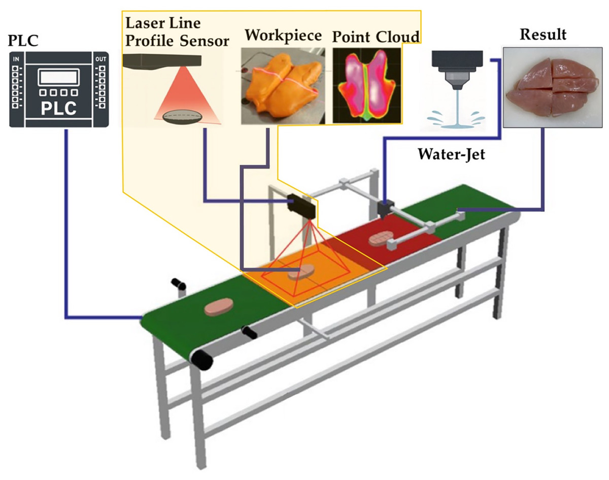
Figure 1: Example of an automated chicken cutting system using high pressure water with an integrated imaging system.
Materials and Methods
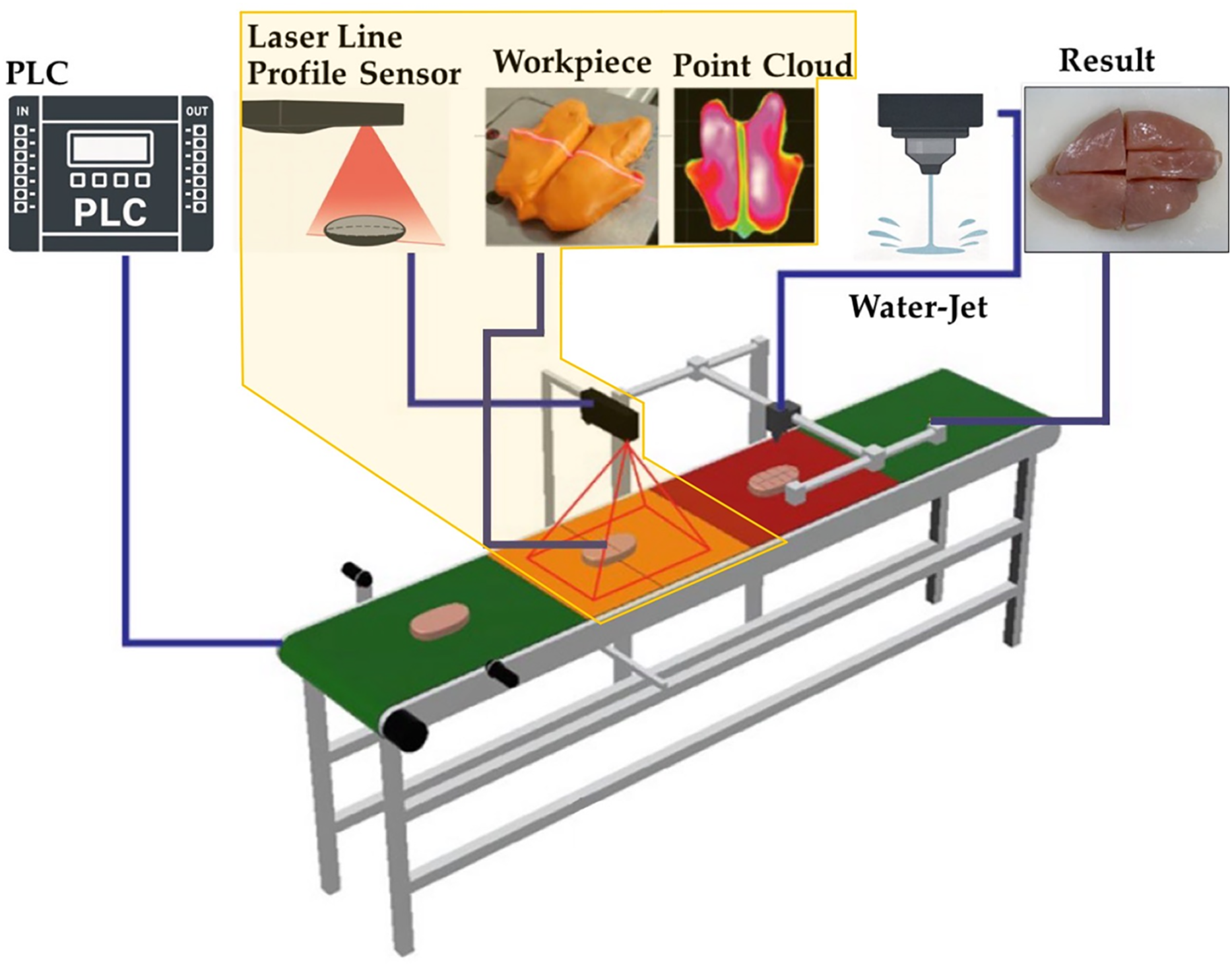
All the equipment was shown in Fig. 2, The machine vision system was set up on the left side of the image and included a laser line profile sensor (Gocator 2140D-3R-R-01-T (LMI Technologies Inc, 2019)), which used laser triangulation technology (França et al., 2005), to acquire 3D point cloud data of the object. The sensor was configured to provide point cloud resolutions of 0.19 mm in the X-axis, 0.5 mm in the Y-axis, and 0.013 mm in the Z-axis. Its field of view ranged from 96 to 194 mm, and it operated at scanning rates between 170 and 5,000 Hz. This data was processed to calculate the object’s volume and determine the cutting lines. This system was controlled using image processing software (HALCON 23.11 Progress Student Edition (MVTec, 2024)). On the right side of Fig. 2 was the evaluation system, which included a cartesian robot (IAI TT-A3-I-2020-10B (Automation, 2024)) equipped with a 1,000 mW laser used solely to project the cutting line onto the object’s surface. This laser was intended for visualization purposes only and was not used to perform any physical cutting. It created visible burn marks on the surface of the material to indicate the cutting locations, which served as guides for manual cutting. The laser setup in this study was designed specifically for experimental use. Due to its power level, it is not currently suitable for direct use in commercial meat processing environments where food safety and thermal impact on biological tissues are critical considerations.
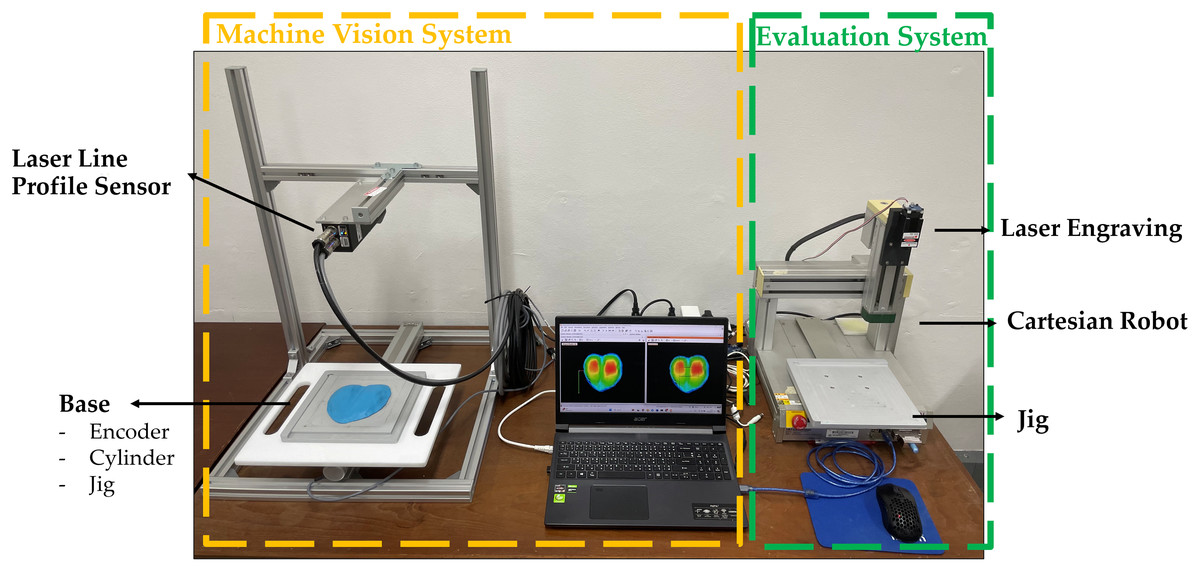
Figure 2: Components of the machine vision system (left side) and evaluation system (right side).
Machine vision system setup
The machine vision system was implemented to acquire point cloud data of meat surfaces, serving as input for the cutting algorithm. This system comprised several key components. The primary component was the laser line profile sensor, which captured point cloud data of the meat surface. The captured data was processed using image processing software (MVTec, 2024), which reconstructed the meat surface into a triangulated point cloud model. This model was subsequently used for algorithmic calculations related to volume estimation and cutting line determination.
To ensure proper scanning and positioning of the meat, the system incorporated a base structure designed to hold the meat securely during the scanning process. The base included an incremental encoder (Kübler KIS40 Series) as shown in Fig. 3A, which was connected to a servo cylinder (RCA ROBO Cylinder: RCA-SA5R-I-20-6-300-A1-R03-ML) in Fig. 3B, which was responsible for moving the object vertically through the scanning field. The servo-cylinder was selected because it allowed integration with the Gocator sensor via the encoder, enabling the vision system to accurately track the displacement of the object during scanning. This ensured synchronization between object movement and laser scanning. Additionally, the base structure consisted of object placing plates (Jig) in Fig. 3C: an upper aluminum plate (190 × 180 mm) to position and hold the meat in place, while a lower aluminum plate functioned as a jig to maintain proper alignment when moving the object to the evaluation system. This jig ensured that the spatial relationship between the scanned point cloud and the physical object was preserved. Consequently, the cutting lines calculated from the point cloud could be accurately mapped to the laser’s focal point during the engraving process, supporting precise laser marking on the actual object surface.
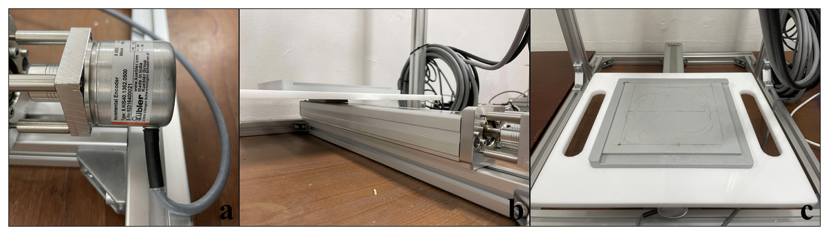
Figure 3: Components of the scanner base.
(A) Incremental encoder used for displacement tracking during scanning. (B) Servo cylinder responsible for vertical object movement and synchronized control with the vision system. (C) Upper and lower aluminum jigs used to fix the object’s position, ensuring consistent alignment between the scanning and evaluation systems.
Installation of the machine vision system
The machine vision system for this study was designed and constructed using an aluminum profile frame (510 mm × 560 mm × 730 mm). This structure supported the installation of the laser line profile sensor and the base for the sliding mechanism, which moved the object during the scanning process, as shown in Fig. 4A. The sliding mechanism provided a scanning range exceeding 150 mm, starting from the encoder installed rail end. The sensor’s laser was aligned at the upper boundary to optimize data capture. The sensor was positioned at 320 mm, producing a 172 mm scanning area, which was later adjusted to a target region of 150 × 150 mm. During scanning, the object moved upward along the sliding rail to ensure accurate data acquisition.
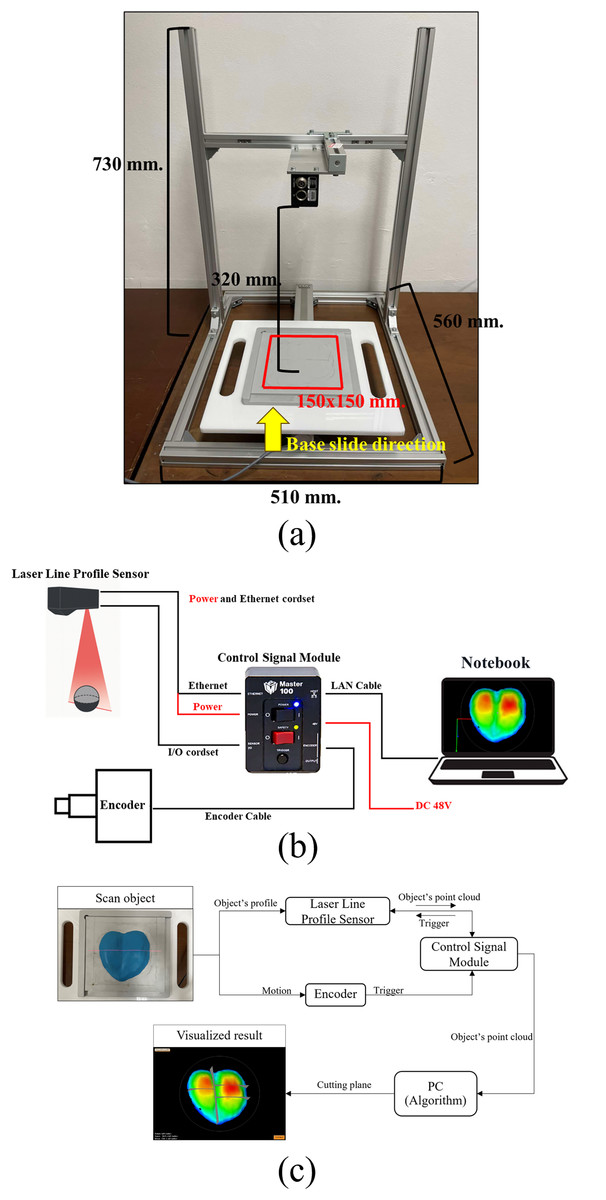
Figure 4: Installation of machine vision systems.
(A) Aluminum frame and sliding object base for scanning. The red-highlighted area indicates the designated region for placing the object during scanning. The yellow arrow shows the scanning direction along the vertical axis as the object moves through the laser line profile sensor’s field of view. (B) System wiring and device connections including laser line profile sensor, encoder, control module, and computer interface used to acquire point cloud data. (C) Block diagram of the machine vision system. Encoder-generated triggers initiate laser profile capture, ensuring uniform spacing. The control module synchronizes sensor and encoder data before transmission to the PC for 3D reconstruction and cutting line computation.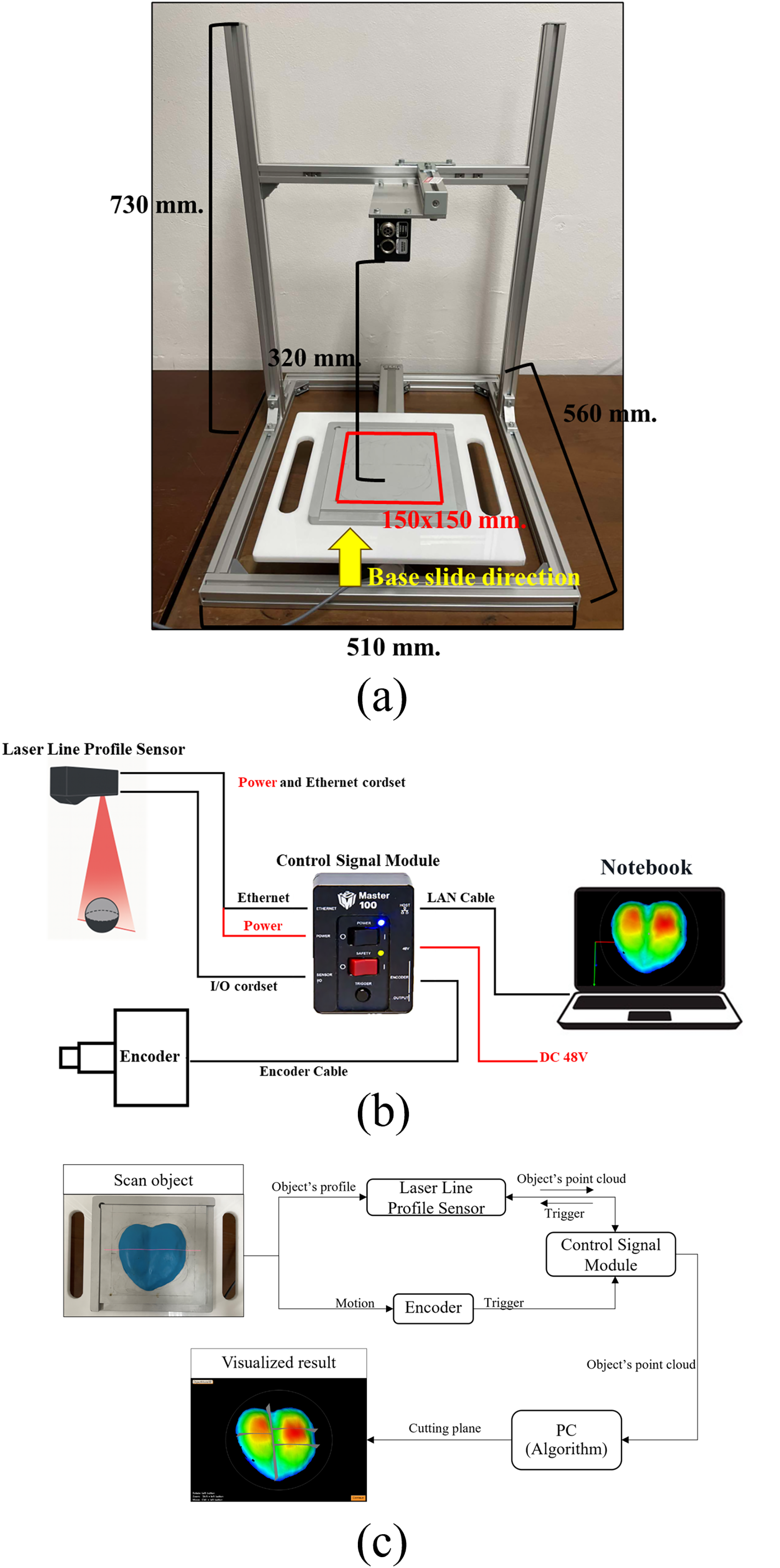
-
(a)
Aluminum frame and sliding object base for scanning. The red-highlighted area indicates the designated region for placing the object during scanning. The yellow arrow shows the scanning direction along the vertical axis as the object moves through the laser line profile sensor’s field of view.
-
(b)
System wiring and device connections including laser line profile sensor, encoder, control module, and computer interface used to acquire point cloud data.
-
(c)
Block diagram of the machine vision system. Encoder-generated triggers initiate laser profile capture, ensuring uniform spacing. The control module synchronizes sensor and encoder data before transmission to the personal computer (PC) for 3D reconstruction and cutting line computation.
To connect the laser line profile sensor to a computer and an encoder, as well as to supply power, a control module (Master 100 (LMI Technologies Inc, 2019)) was used. Figure 4B illustrates the interconnection of the sensor, encoder, control module, and computer. The I/O cordset linked the sensor’s I/O and Power/LAN ports to the control module, enabling signal transmission to the encoder. The power and Ethernet cordset connected the sensor to both the power supply and the computer, while the encoder’s signal cable was linked to the control module. Acting as a central hub, the control module supplied power and transmitted sensor data to the computer via Ethernet. The vision processing software, utilizing the Generic Interface for Cameras (GenICam) protocol, processed the data collected from the sensor, ensuring seamless hardware software communication.
To clarify the data communication and processing workflow, Fig. 4C presents a block diagram of the machine vision system. The process begins with the laser line profile sensor, which projects a laser line onto the surface of the object placed on a jig. A trigger event is required for the sensor to capture each profile image. In this setup, the trigger is generated by an incremental encoder, which detects motion as the object moves along the scanning axis. Once triggered, the laser is strobed, and the sensor camera captures a single image. This image is internally processed by the sensor to yield a profile (range/distance information). These profiles are sequentially collected to reconstruct a full 3D point cloud of the object. The control signal module receives inputs from both the sensor and the encoder and acts as a synchronization hub, managing data flow and power supply. Finally, the data is transmitted to the PC, where image processing software executes the cutting algorithm to calculate cutting lines.
The total processing time from initiating the scan to generating cutting lines, when dividing the object into 2 to 6 segments, was approximately 20 s. This duration was divided into three stages: first stage 10 s for initializing the system and establishing the connection between the laser line profile sensor and image processing software upon pressing the “Run” command, second stage 5 s for moving the object through the scanning range and rendering the point cloud, and third stage approximately 2–3 s for computing the cutting line positions using image processing software, excluding additional time for visual verification and display.
The laptop used in this research had the following specifications:
Processor: AMD Ryzen 5 5500U
Graphics Card: Radeon Graphics 2.10 GHz
Random Access Memory (RAM): 16 GB DDR4 3,200 MHz
Storage: SSD M.2 512 GB
Operating system: Windows 11
Cutting algorithm
The core of this research was developing an algorithm to determine cutting lines that divide meat into equal weight portions. The algorithm used volume segmentation based on point cloud data from the machine vision system. It calculated the total volume and systematically divided it into equal parts by determining optimal cutting lines. Assuming the solid has a constant density, the algorithm used volume as a substitute for mass, ensuring that each equal volume section also had equal mass. The algorithm consisted of two main processes: volume computation and cutting line determination.
Volume computation
The point cloud data was collected using the laser line profile sensor, which captured point cloud data from the meat’s surface and transmitted the information as images to vision processing software. Each pixel in the captured image contained 3D coordinate data, which was extracted through programmed processing to reconstruct the full point cloud representation of the object (MVTec, 2022), as illustrated in Fig. 5. However, due to occlusions, surface reflections, or scanning limitations, certain regions of the point cloud contained missing data. To resolve this issue, the built-in Gap Filling function of the laser line profile sensor was employed. This gap filling method reconstructs missing data points by either selecting the lowest values from nearest neighbors or performing linear interpolation between neighboring points. Gap filling was applied along both the X- and Y-axes using a window size of x = 8 mm and y = 5 mm to ensure surface completeness. In addition, the built-in smoothing filters of the laser line profile sensor were used to reduce noise and enhance surface continuity. Smoothing operates by replacing each data point with the average of that point and its nearest neighbors within a defined window. In this study, smoothing was applied in both directions, with the X axis processed first followed by the Y axis, using a smoothing window size of x = 2 mm and y = 2 mm. This preprocessing step resulted in a cleaner, more consistent point cloud for subsequent volume computation and segmentation (LMI Technologies Inc, 2019).
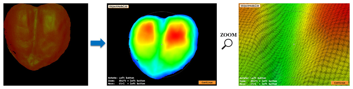
Figure 5: The image on the left side was the object’s image from a sensor converted into a point cloud on the right side.
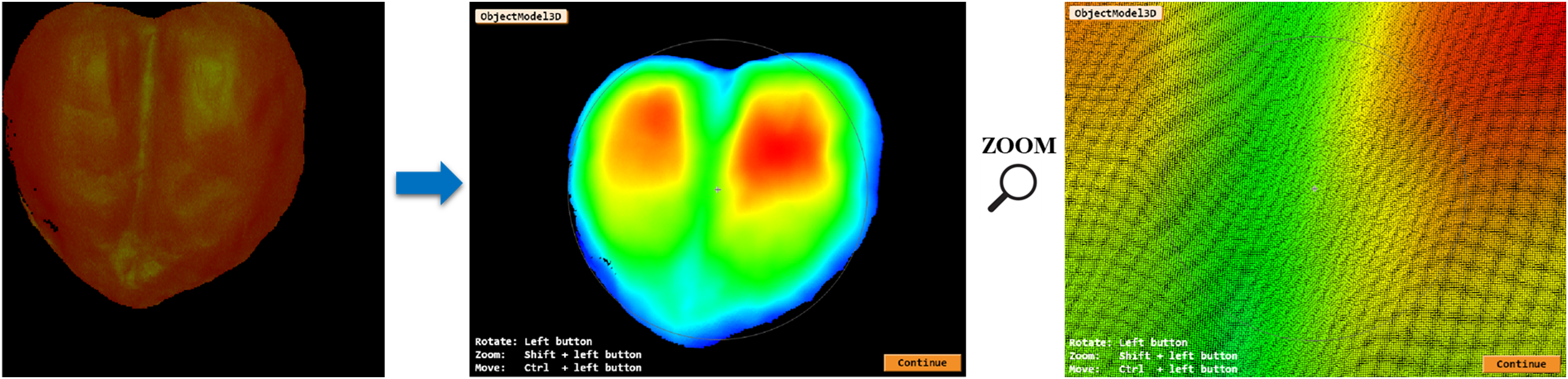
Once the point cloud was obtained, the system applied Delaunay triangulation (Cheng, Dey & Shewchuk, 2012), creating a triangular surface mesh to model the 3D shape of the meat. This method ensured that each triangle was formed by connecting adjacent points, allowing for an accurate representation of the surface topology as illustrated in Fig. 6. The total volume of the object was then computed by summing the volumes of vertical triangular prisms formed between each triangle in the surface mesh and the reference base plane as illustrated in Fig. 7. For each triangle , the volume was calculated using Eq. (1).
(1) where
= the area of each triangle on the surface mesh,
= the average vertical distance (height) from the triangle’s face to the base plane.
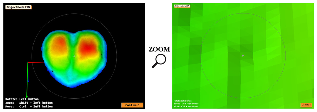
Figure 6: Triangulated mesh generated from the point cloud using Delaunay triangulation.
The mesh is used for volume computation.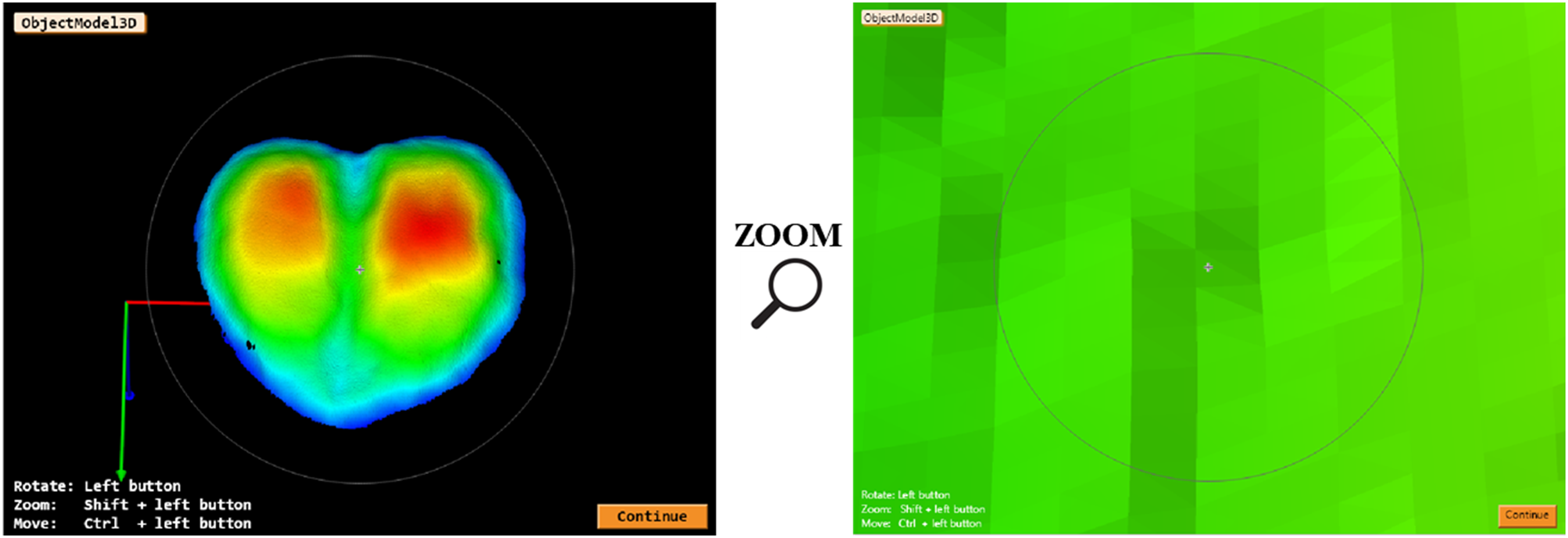
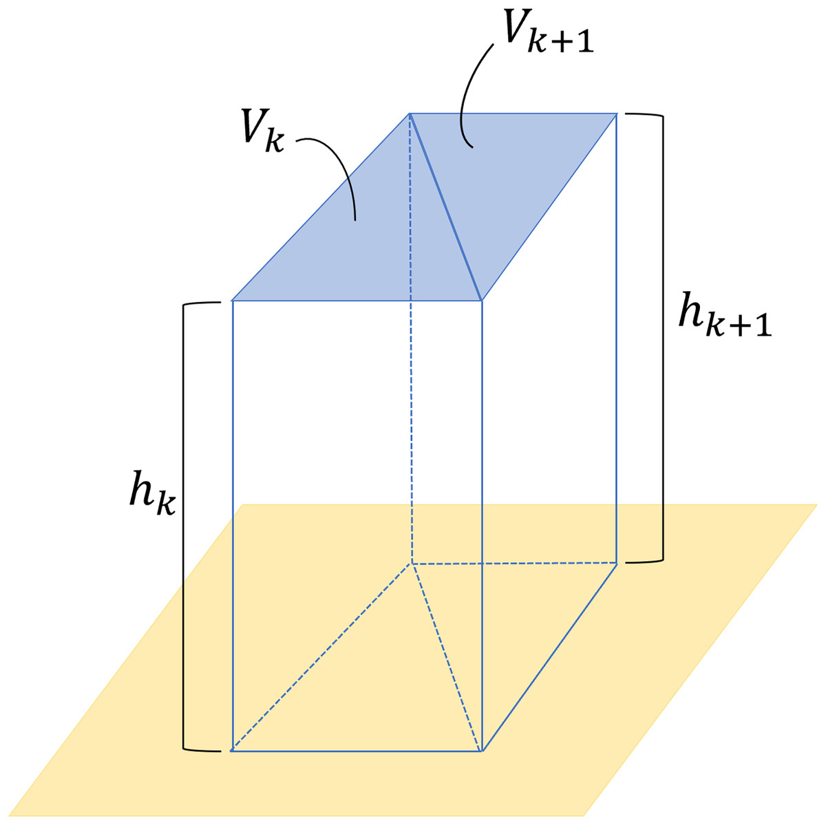
Figure 7: Triangular prisms formed between each triangle in the surface mesh and the reference base plane.
The volumes of these prisms are summed to estimate the total object volume.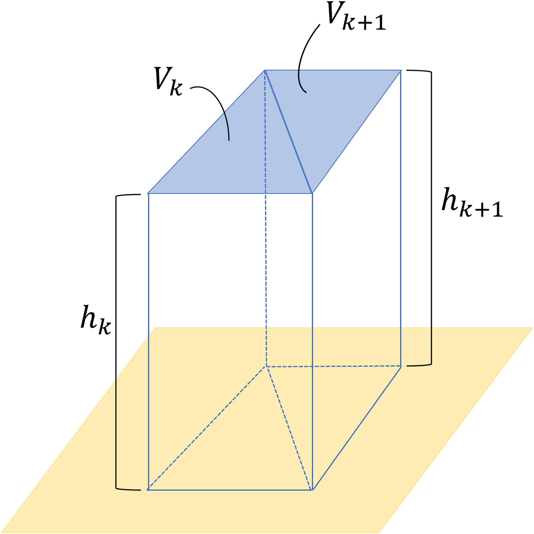
The total volume of the object is then approximated by summing the volumes of all such prisms, as shown in Eq. (2).
(2)
This total volume was later used in the cutting line determination process to ensure equal weight portions. Once the surface was modeled, the total meat volume was estimated by integrating the surface mesh over a defined reference plane.
Cutting line determination
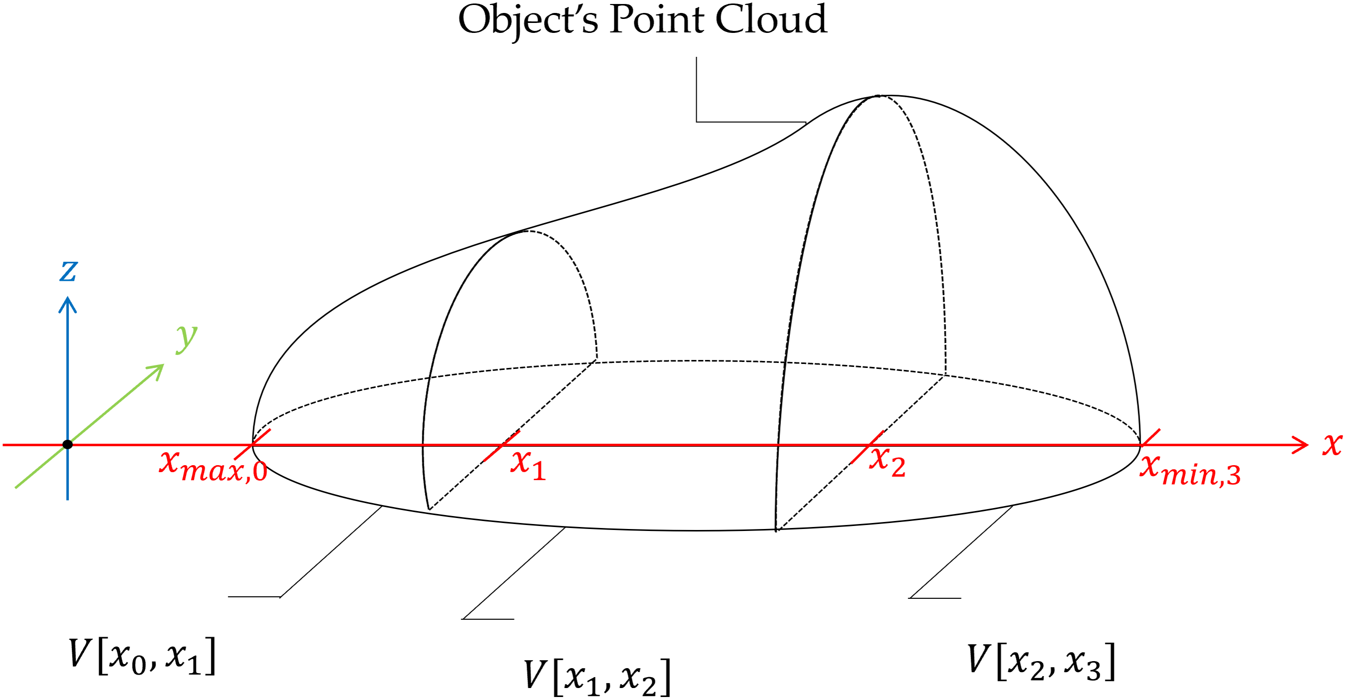
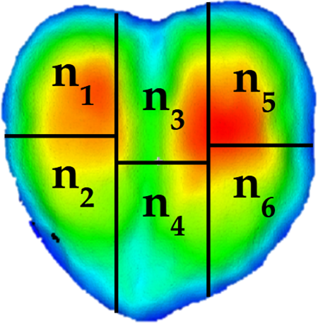
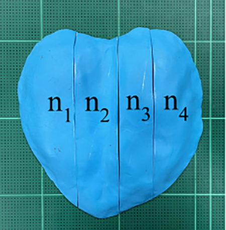
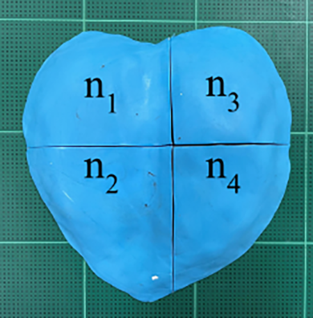
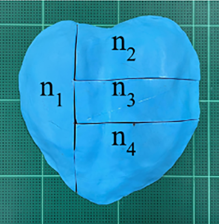
After calculating the object’s volume, a volume-based method was applied to determine the cutting lines. These lines were defined in two ways: either as vertical cuts only or as a combination of vertical and horizontal cuts, ensuring that all segments had equal weight and volume. The position of vertical cutting lines were represented by the variable , while the position of horizontal cutting lines were represented by For example from Fig. 8, in the case where the object was divided using vertical cuts, the algorithm determined and so that the volume of each segment ( for ) remained equal.
![An object segmented into three parts using vertical cutting lines, where
${\bf V}\left[ {{{\bf x}_0},\; {{\bf x}_1}} \right] = {\bf V}\left[ {{{\bf x}_1},\; {{\bf x}_2}} \right] = {\bf V}\left[ {{{\bf x}_2},\; {{\bf x}_3}} \right]$V[x0,x1]=V[x1,x2]=V[x2,x3]
.](https://dfzljdn9uc3pi.cloudfront.net/2025/cs-3377/1/fig-8-2x.jpg)
Figure 8: An object segmented into three parts using vertical cutting lines, where .
The step-by-step process is explained through the pseudo code provided below.
01 1. INITIALIZATION
02 Define (number of vertical segments)
03 Define array (number of horizontal segments for each vertical segment)
04 Calculate total segments
05 Calculate Volume each piece
06 For volume of each vertical segment i, compute
07
08 2. VERTICAL SEGMENTATION
09 Retrieve the x-coordinates from the 3D object
10 Determine and
11
12 For to :
13 If is not the last vertical segment:
14 Initialize and
15 While:
16 Compute
17 Select object points with x-values between current and
18 Compute the volume of this segment
19 If :
20 Break the loop
21 Else if ]:
22 Set
23 Else:
24 Set
25 End While
26 Record vertical cut position:
27 Segment the object using the plane at
28 Save the portion as
29 Update current =
30 Else: (For last part)
31 Select points from current to and compute the volume
32 Save the segmented vertical part as
33 End If
34 End For
35
36 3. HORIZONTAL SEGMENTATION (For each vertical segment)
37 For to (Each vertical segment):
38 Retrieve the y-coordinates from
39 Determine and
40
41 For j from 0 to :
42 If j is not the last horizontal segment:
43 Initialize and
44 While:
45 Compute
46 Select object points with y-values between and
47 Compute the volume of this slice
48 If
49 Break the loop
50 Else if :
51 Set
52 Else:
53 Set
54 End While
55 Record horizontal cut position:
56 Segment the vertical part using the plane at
57 Save the portion as
58 Update
59 Else: (For last part)
60 Select points from to and compute the volume
61 Save the segmented horizontal part as
62 End If
63 End For
64 End For
65
66 # 4. OUTPUT
67 Output the vertical cut positions ( ) and horizontal cut positions ( )
68 Final segmented parts are stored in and
69 For each cutting line (vertical and horizontal), extract the intersection with the 3D model
70 Save each intersection plane as a separate .PLY file
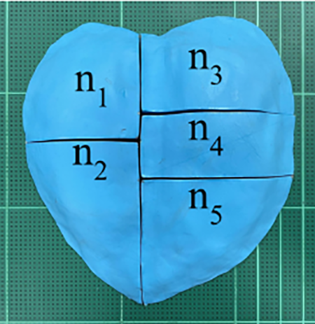
Initialization (Lines 01–06): The algorithm defines the number of segments along the vertical ( ) and horizontal ( ) directions, calculates the total number of final segments ( ), and determines the target volume for each segment ( ). For each vertical segment, a target volume ( ) is computed based on its corresponding horizontal divisions.
For example, if = 3 and = [2, 3, 1], this configuration divides the object into three vertical regions. The first region is subdivided into two horizontal slices, the second into 3, and the third into 1, resulting in a total of = 6 segments. The total object volume is divided equally across these six segments, such that each piece should have volume = Total Volume/6. Consequently, the volume allocated for each vertical segment becomes .
Vertical segmentation (Lines 08–34, Fig. 9): In this step, the goal is to divide the 3D object into several vertical parts along the x-axis, each having a specific volume depending on . The algorithm first identifies the object’s minimum and maximum x-coordinates ( , ), indicated by the dashed lines in Fig. 9, left. It then searches for a cutting position (shown as the red line in Fig. 9, left) such that the volume between and closely matches the target (shown as the green block in Fig. 9, right). If the volume is too large, it adjusts to a smaller position ( ); if too small, it moves to a larger position ( ). When a position is found where the volume is close enough to the target, the position and point cloud are saved as and , respectively. The process repeats for each vertical segment until all parts are defined, with the last segment covering everything up to .
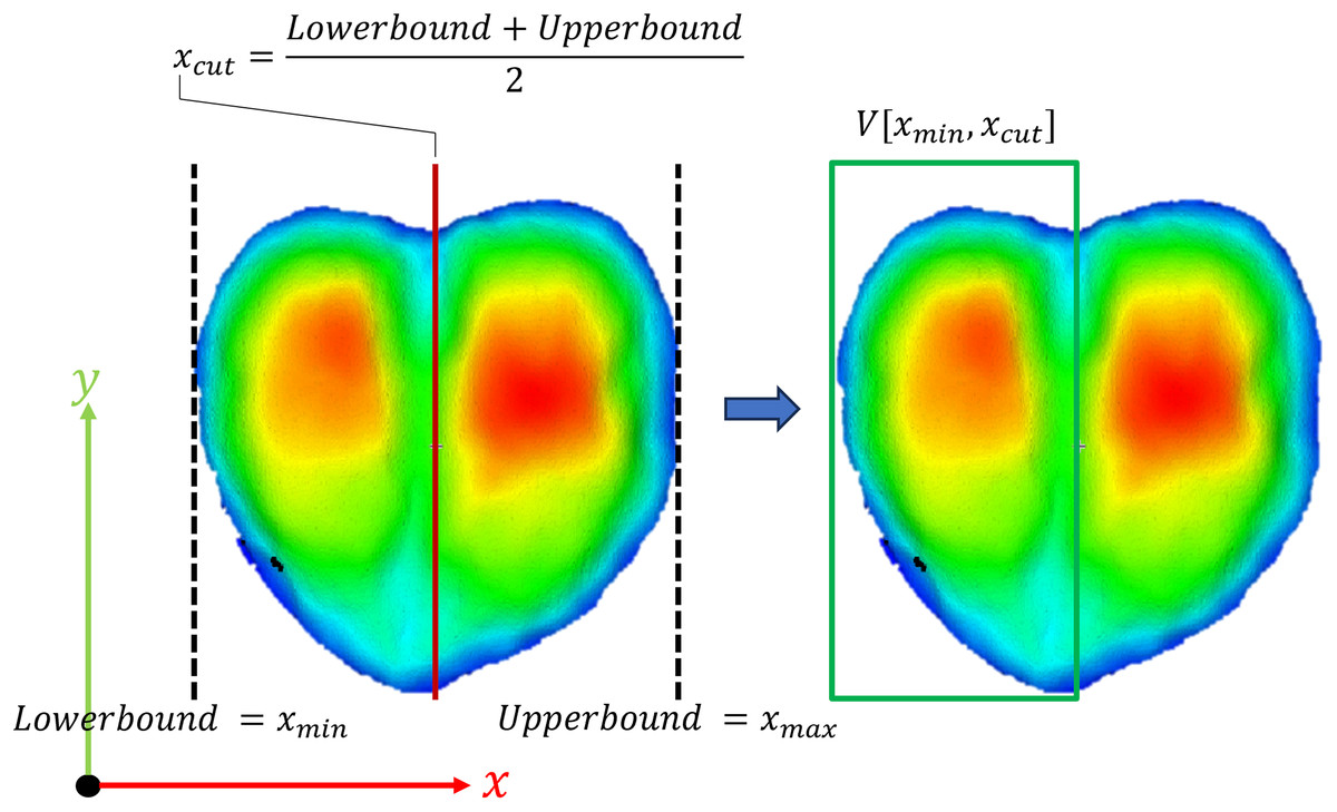
Figure 9: Point cloud being segmented during the vertical segmentation.
Horizontal Segmentation (Lines 36–64, Fig. 10): After dividing the object vertically, each vertical part is further divided horizontally along the y-axis. For each vertical part that is saved in , the algorithm first identifies the object’s minimum and maximum y-coordinates ( , ), indicated by the dashed lines in Fig. 10, left. It then searches for a cutting position (shown as the red line in Fig. 10, left) such that the volume between and closely matches the desired volume. If the volume is too large, the position is adjusted closer to a smaller position ( ); if too small, it moves to a larger position ( ). When the volume is close enough to the target, the position and point cloud is saved as and respectively. This process is repeated until all horizontal lines for each vertical part are defined, with the last slice covering everything up to .
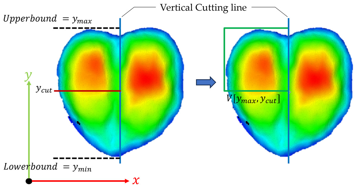
Figure 10: Point cloud being segmented during the horizontal segmentation.
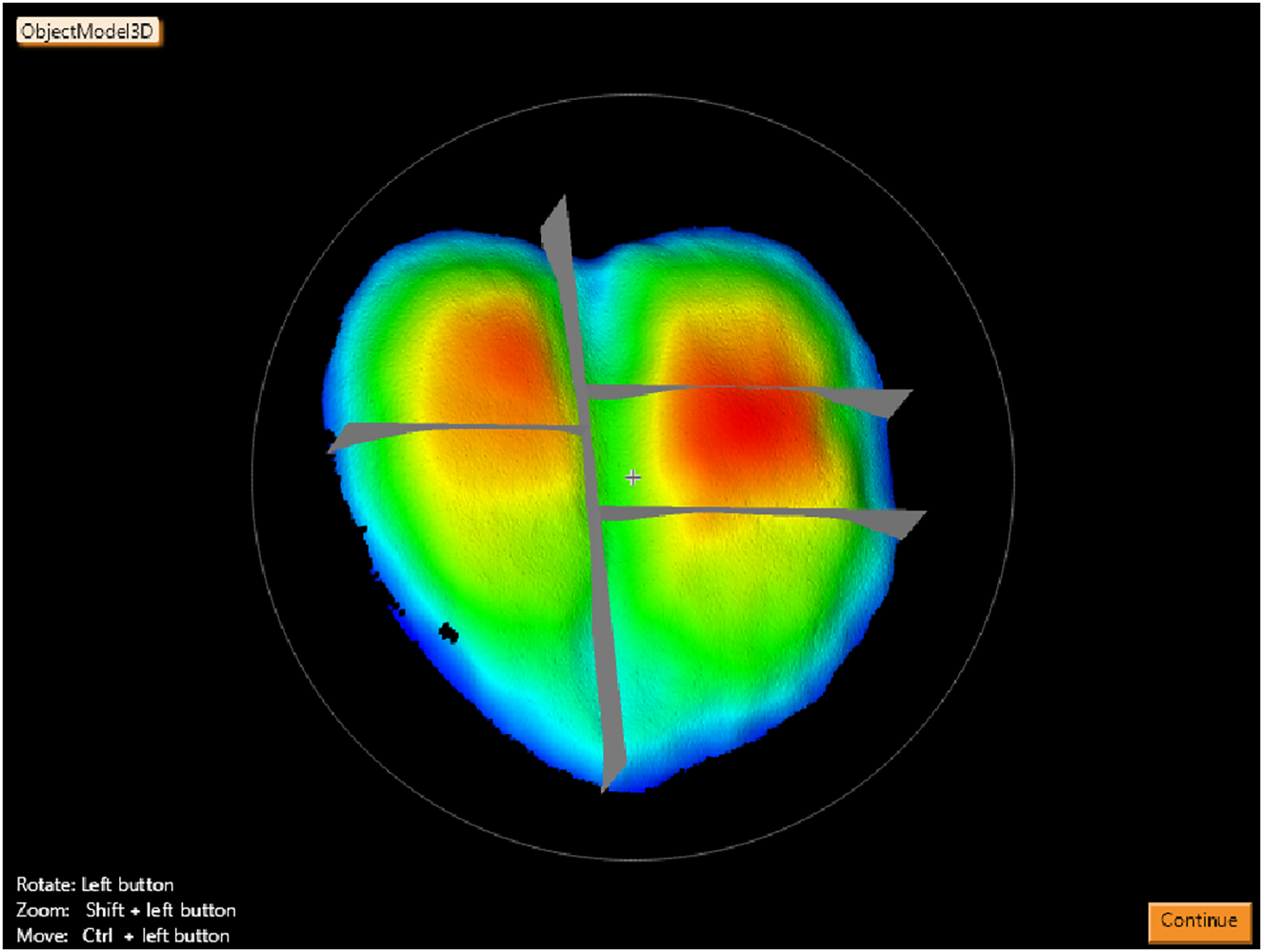
Output (Lines 65–68): Finally, the algorithm outputs the positions of the cutting lines along the x-axis ( ) and y-axis ( ), and the segmented parts ( and ) are stored for further use. For example, the cutting lines shown in Fig. 11 are desired, the values that must be set are and .
![Result of cutting algorithm (nv = 2 and nh = [2, 3]).](https://dfzljdn9uc3pi.cloudfront.net/2025/cs-3377/1/fig-11-2x.jpg)
Figure 11: Result of cutting algorithm (nv = 2 and nh = [2, 3]).
After computing these cutting lines, the algorithm generates 3D intersection planes that represent the actual cutting surfaces. Each intersection is extracted and saved individually as a .PLY (Polygon File Format) file. In the evaluation phase described in ‘Cutting Algorithm Evaluation’, these PLY files are used to project cutting lines onto the sample surface via a laser engraving module.
Cutting algorithm evaluation
The following section presents the equipment and methodologies used for evaluating the cutting algorithm. This includes a detailed overview of the hardware and software components necessary for system setup. Additionally, the evaluation methods were outlined to assess the algorithm’s performance in terms of accuracy, repeatability, reproducibility, and segmentation efficiency.
Setup system for evaluation
To verify that the cutting lines generated by the proposed method could accurately divide the object into equal-weight portions, laser engraving was used to apply the cutting lines onto the object’s surface. This technique burned markings along the calculated lines, providing a clear visual representation for further analysis and evaluation. The setup consisted of three main components as shown in green area of Fig. 2: a cartesian robot, which enabled movement along the X, Y, and Z axes; a laser engraving module, mounted on the robot to mark the cutting lines on the meat surface; and a movable base plate (jig), which ensured accurate positioning between the machine vision system and the evaluation system.
Evaluation method
Many test samples were required to comprehensively evaluate the algorithm’s capability to divide objects into equal-weight portions. To minimize the loss of raw chicken meat and reduce experimental costs, modeling clay was selected as the primary test material during the initial evaluation stages. Clay samples allowed repeated trials under controlled conditions while maintaining consistent shape and weight. The evaluation process incorporated multiple statistical methods, including verification of the algorithm’s accuracy in object volume calculation, one-way ANOVA to assess the effect of different cutting patterns on segmentation accuracy, and Gage R&R analysis to quantify measurement system reliability across multiple segments. Following these preliminary tests, the algorithm was validated on actual chicken breast and fish fillets to confirm its practical applicability under realistic processing conditions.
Figure 12 illustrates the data collection process in preparation for the evaluation procedure, starting with scanning the object and determining cutting lines using the machine vision system. Once the computed cutting lines were identified, they were projected onto the object surface using the laser engraving module mounted on the cartesian robot. The system first received the cutting coordinates from the cutting algorithm and converted them into precise movement commands for the robot. The robot then positioned the laser over the designated cutting lines and initiated the engraving process. Figure 13A shows that the engraved cutting lines serve as guides for the subsequent cutting process, where operators used knives to follow the marked lines and divide the object accordingly. After the object was cut, each piece was weighed to collect data for further evaluation, with the sequence of each piece being recorded, as shown in Fig. 13B.
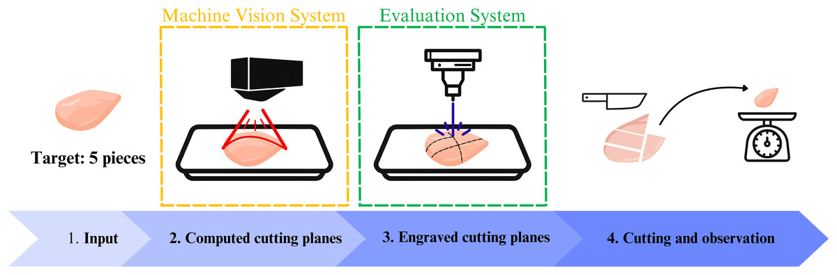
Figure 12: Step-by-step data collection process.
The yellow frame highlights the machine vision system, which performs scanning and segmentation. The green frame indicates the evaluation system, where the calculated cutting lines are applied and verified through laser projection and manual cutting.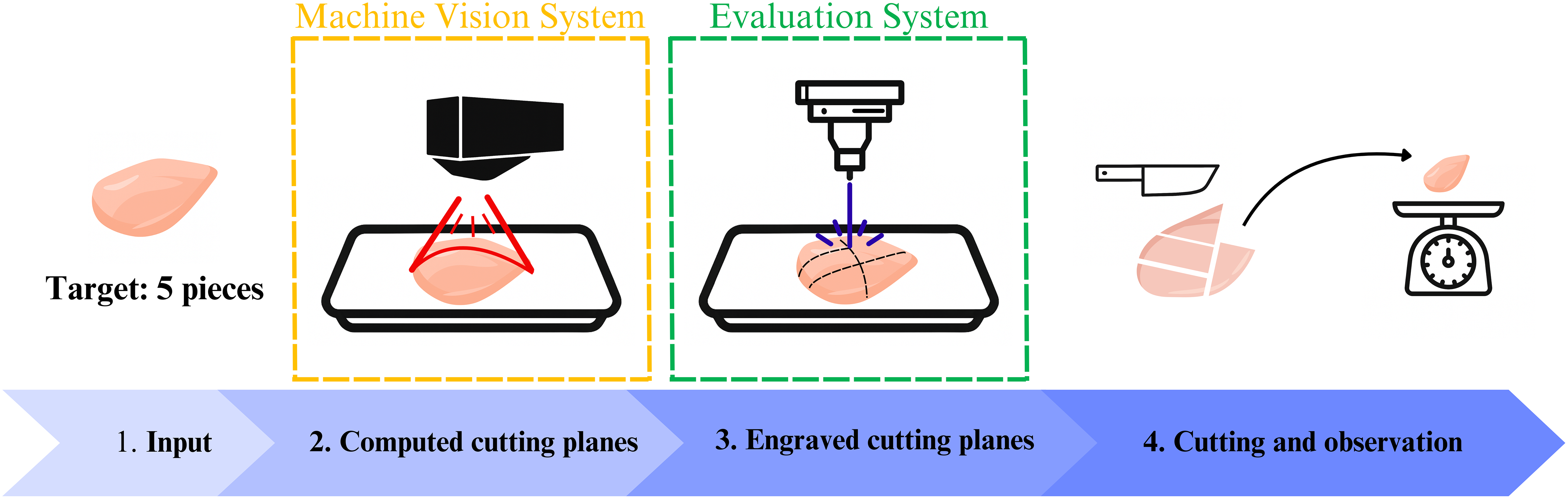
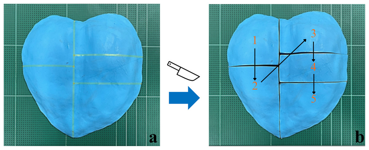
Figure 13: Cutting and observation procedure.
(A) Object marked with laser burning. (B) Object manually cut along the laser marked lines, with sequential numbering example for data collection.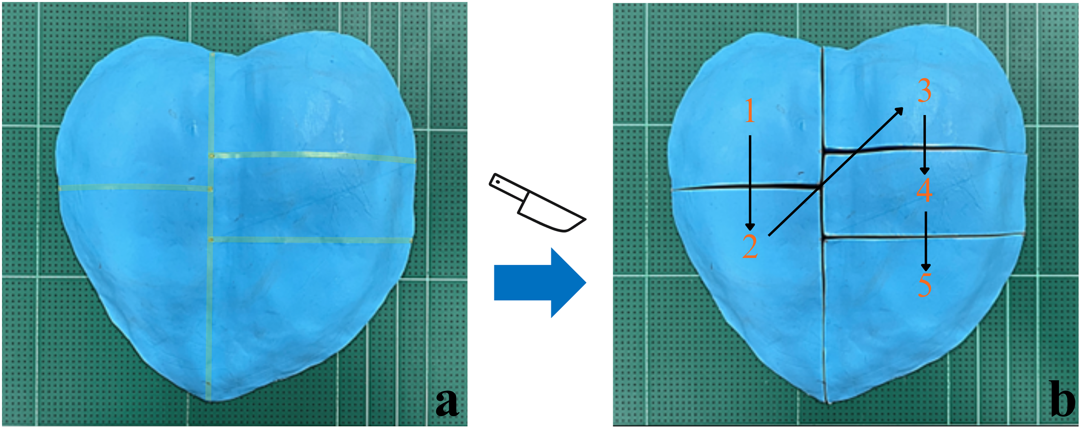
The experiments are as follows:
-
(1)
Segmentation errors and limitations in point cloud volume calculation
This experiment was conducted to verify that the volume-segmentation algorithm partitions each object into n segments matching the target volume.
-
(2)
Testing different cutting patterns
To evaluate how cutting configurations affect weight uniformity, we prepared modeling clay samples of 200 g and applied five cutting patterns. Each pattern was repeated five times (Total 25 samples). Cutting lines were generated by the algorithm and projected via laser for manual separation and weighing, following the data-collection workflow in Fig. 12. The primary outcomes were MAE and percentage MAE (%MAE), computed as in Eqs. (3), (4). Data screening included the Kolmogorov–Smirnov test for normality and Levene’s test for homogeneity. Group differences in MAE across cutting patterns were analyzed using one-way ANOVA. (3) (4) where:
= Mean Absolute Error
= Measured weight of the object segment
x = Expected weight per segment
n = Number of segments the object is divided into
A one-way ANOVA test was conducted to determine whether significant differences existed between the cutting patterns in terms of MAE. This analysis aimed to ascertain the extent to which different cutting configurations influenced segment weight consistency. Before conducting ANOVA, data normality was validated using the Kolmogorov-Smirnov test, while Levene’s test was applied to confirm the homogeneity of variance (Massey, 1951). Sample size (N) was determined with G*Power (Faul et al., 2007) for a one-way ANOVA. The study was structured with the following parameters: significance level (α) = 0.05, power = 0.8, and five experimental groups. The effect size (Cohen, 2013) used in this study (f = 0.852) was computed in G*Power using Eq. (5), based on group means obtained from a pilot study, leading to a minimum total sample size of 25 pieces, ensuring five repetitions per cutting pattern. (5) where:
Sample size for each group
Mean of each group
Grand mean
Number of groups
Standard deviation within groups
-
(3)
Gage R&R (Gauge Repeatability and Reproducibility)
Gage R&R is a statistical method used to evaluate the quality of a measurement system by assessing its repeatability (the consistency of measurements taken by the same instrument under the same conditions) and reproducibility (the consistency of measurements taken by different operators or across different groups). Typically, a Gage R&R study begins by selecting multiple test samples and multiple operators. Each operator then measures each sample multiple times to assess variability. In this thesis, Gage R&R was applied to analyze the weight of the first modeling clay piece after it had been cut.
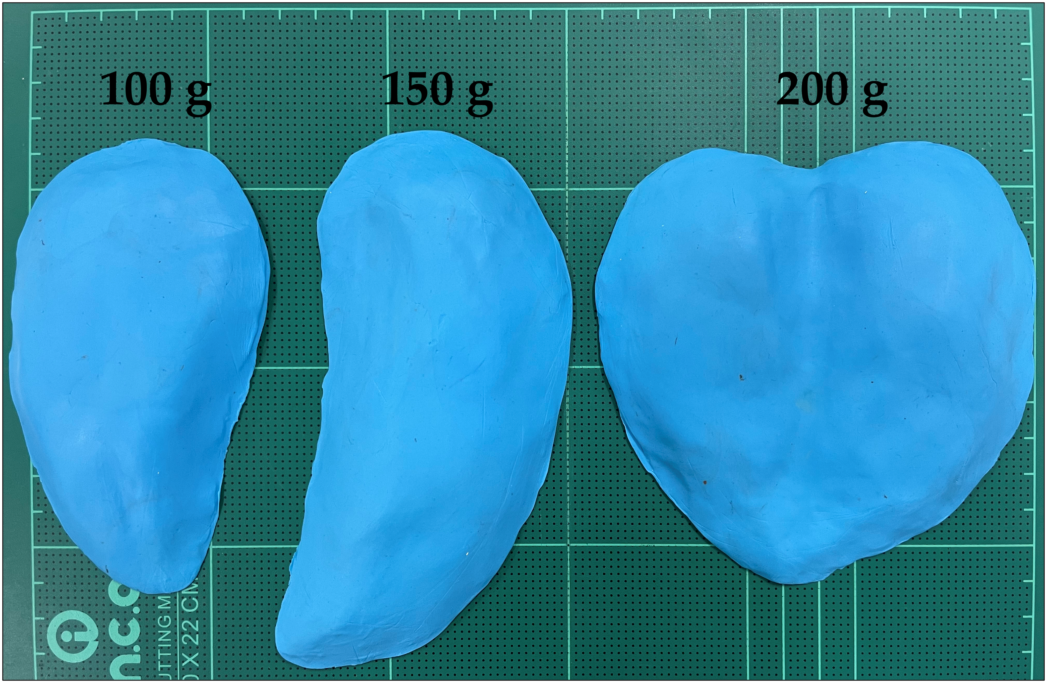
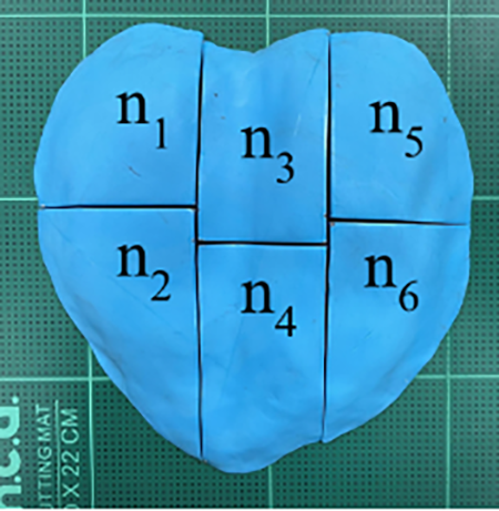
The data collection process involved multiple steps to ensure the accuracy and reliability of the weight measurements after the cutting process. First, 81 modeling clay samples of 100, 150, and 200 g were prepared and molded into uniform shapes to minimize external variations, as shown in Fig. 14. Each sample was then divided into 4, 5, or 6 pieces using algorithm-generated cutting lines. To simulate variability in operator placement commonly found in industrial environments, the samples were intentionally positioned in three different orientations before scanning. For example, the 100 g samples were rotated approximately 90° and 120° from their initial position, the 150 g samples were laterally shifted by ±20 mm, and the 200 g samples were rotated to 90° and 180°, with minor displacements up to ±5 mm and angular variations up to ±10°. Weight measurements were collected for the first three segments (Segment 1–3) of each sample to evaluate the consistency and reliability of the system across different portions of the object. Each segment was weighed using a precision scale after manual cutting along the engraved paths, and the data were recorded in a structured sequence.
-
4)
Real meat portioning test
To validate the performance of the developed cutting algorithm on actual food products, experiments were conducted using chicken breast and fish fillets as test materials. The aim was to evaluate the algorithm’s capability to portion real meat into equal-weight segments.
For each meat type, 30 individual samples were used (total of 60 samples). The samples were randomly allocated into three cutting configurations:
-
•
4 segments (chicken breast 10 samples, fish 10 samples)
-
•
5 segments (chicken breast 10 samples, fish 10 samples)
-
•
6 segments (chicken breast 10 samples, fish 10 samples)
-
The initial weights of the meat pieces varied within each group to represent realistic processing conditions. The machine vision system scanned each sample to acquire point cloud data, and the cutting algorithm computed vertical and horizontal cutting lines to achieve equal-volume segmentation. The calculated cut positions were projected onto the meat using the laser marking system of the evaluation setup, after which manual cutting was performed along the marked lines. Following cutting, each segment was weighed. The primary performance metric was the percentage mean absolute error (%MAE) between the actual and target weights, calculated as Eqs 3 and 4. The standard deviation (SD) of segment weights and the maximum and minimum %MAE values within each group were also recorded.
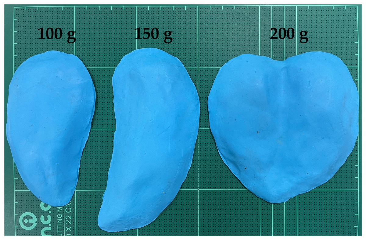
Figure 14: Modeling clay samples of 100, 150, and 200 g.
Results
Segmentation errors and limitations in point cloud volume calculation
Table 1 presents errors resulting from the volume segmentation of the point cloud. Column 2 displays the volume calculated from the entire point cloud of the object, while column 3 represents the desired volume (Vi), obtained by dividing the total volume from column 2 by the number of segments required. Ideally, the point cloud should be segmented to match the volume in column 3. However, the actual segmented volume deviates from the desired value, as shown in columns 4–9, which indicate the percentage difference. A negative value means the segmented volume was less than the desired volume, whereas a positive value indicates an excess. Most values exhibit a deviation within ±0.5%, as the first condition limits the acceptable difference to 0.5%. However, some segments exceed −0.5%. The last column of Table 1 presents the sum of total segmented volume derived from the calculated cutting lines, which was consistently lower than the total volume computed from the complete point cloud of the object.
| Volume (×103 mm3) |
Vi (×103 mm3) |
%Error of volume | Sum (×103 mm3) |
||||||
|---|---|---|---|---|---|---|---|---|---|
| n1 | n2 | n3 | n4 | n5 | n6 | ||||
 |
115.11 | 28.77 | 0.41% | −0.16% | −0.09% | −3.16% | 114.39 | ||
 |
111.08 | 22.22 | 0.08% | 0.31% | −0.19% | −0.37% | −2.64% | 110.45 | |
 |
117.01 | 19.50 | 0.17% | −0.30% | 0.06% | −0.86% | 0.27% | −2.43% | 116.41 |
Testing different cutting patterns
Table 2 presents various statistical measures used to evaluate the accuracy of weight distribution in segmented objects. Columns 1 to 5 display the post-cut appearance of the modeling clay, the desired number of segments, the actual weight per segment, the median (Median), and the standard deviation (SD), respectively. Column 6 represents the MAE, which was calculated by averaging the absolute deviations of segment weights from the expected values, as defined in Eq. (3). Column 7 shows the %MAE, computed using Eq. (4). Columns 8, 9, and 10 provide the maximum and minimum weights obtained, the largest deviation from the expected weight, and the percentage error corresponding to that deviation, respectively. These metrics collectively assessed the algorithm’s effectiveness in achieving uniform weight distribution across all segmented pieces.
| Number of part | Mass/n (g) | Median (g) | SD (g) | MAE (g) | %MAE | Max & Min (g) | Max error (g) |
% Max error | |
|---|---|---|---|---|---|---|---|---|---|
 |
4 | 50 | 50.9 | 2.1 | 1.8 | 3.54% | 52.4–45.6 | 4.4 | 8.8% |
 |
4 | 50 | 50.2 | 1.4 | 1.2 | 2.44% | 52.4–45.7 | 2.3 | 4.6% |
 |
4 | 50 | 49.8 | 1.7 | 1.3 | 2.62% | 53.2–47.4 | 3.2 | 6.4% |
 |
5 | 40 | 39.9 | 1.1 | 1.1 | 2.78% | 42.2–37.9 | 2.2 | 5.5% |
 |
6 | 33.3 | 33.3 | 1.5 | 1.2 | 3.50% | 36.4–30.8 | 3.1 | 9.3% |
Table 2 demonstrates the variety of cutting patterns that can be used to divide clay, including both vertical and horizontal cuts or vertical cuts alone. The values across different cutting patterns were similar. The cutting pattern with the highest error margin was found in the first row, where the clay was divided into four pieces, with an expected weight of 50 g per piece. After repeating the process five times, a total of 20 pieces were obtained. The median weight was 50.9 g, with a standard deviation of 2.1 g. The MAE was 1.8 g, corresponding to a percentage MAE of 3.54%. The maximum and minimum weights recorded were 52.4 and 45.6 g, respectively, with the highest absolute error measured at 4.4 g and the highest percentage error at 8.8%.
One-way ANOVA for cutting pattern analysis
The analysis was based on the data presented in Table 2. Before conducting ANOVA, data normality was validated using the Kolmogorov-Smirnov test, while Levene’s test was applied to confirm the homogeneity of variance (Massey, 1951). Results indicated that the data set met the assumptions necessary for ANOVA.
The result of ANOVA test in Table 3 revealed statistically significant differences among at least one pair of cutting patterns, F(4, 20) = 6.029, p = 0.002.
| MAE | Sum of squares | df | Mean square | F | Sig. |
|---|---|---|---|---|---|
| Between groups | 2.132 | 4 | 0.533 | 6.029 | 0.002 |
| Within groups | 1.768 | 20 | 0.088 | ||
| Total | 3.900 | 24 |
Gage R&R
To analyze the sources of variation, a Two-Way ANOVA was performed both with and without interaction effects. To fully interpret the results, the following definitions explain what each variance component represents in this study:
Part (Sample Variation): The variation caused by differences in the weight of the first cut segment of the clay. This reflects the actual variation in clay sample weights when divided into equal portions.
Operator (Positioning Variation): The variation caused by differences in the placement of the clay sample before scanning. This accounts for the potential impact of object positioning on the accuracy of the weight distribution.
Operator * Part (Interaction Effect): The variation caused by the interaction between sample weight and its placement. This occurs if different sample weights produce significantly different results depending on their placement.
Error/Repeatability: The variation that cannot be explained by part, operator, or interaction effects. This includes all unexplained sources of measurement variation.
From Table 1A, the interaction term (Part * Operator) had a p-value of 0.149, which is not statistically significant, confirming that sample weight differences were not influenced by object placement. Since the interaction effect is above the 0.05 threshold, it was removed in a second ANOVA analysis without interaction.
Without interaction Table 2A, the part variance remains significant (p = 0.000), confirming that weight variation primarily comes from differences in sample mass. The Operator p-value remains non-significant (p = 0.907), reinforcing that sample placement did not impact measurement accuracy. The removal of interaction did not change the significance of the results, confirming that the weight differences were due to part variation rather than measurement system inconsistencies.
The Gage R&R analysis was performed to quantify how much of the overall weight variation was due to measurement system errors compared to actual differences in sample composition. Each variance component analyzed in this study represents a different source of measurement variability
Total Gage R&R: The combined variability resulting from both Repeatability and Reproducibility, representing the total measurement system variation.
Repeatability: Variation in the first cut segment’s weight when the same number of divisions and same positioning are used multiple times. This includes errors from clay molding, cutting line computation, point cloud generation, laser projection, and manual cutting.
Reproducibility: The variability in the weight of the first cut segment when the same number of divisions is used, but the clay sample is placed in different scanning positions. This reflects how much positioning affects the accuracy of the system.
Part-to-Part Variation: The variability in the weight of the first cut segment when the number of divisions differs across different samples. This represents the actual differences in weight caused by different cutting configurations.
From Table 4, the total Gage R&R variance was 7.04%, which is within the commonly accepted limit (<10%) (Automotive Industry Action Group, 1990), confirming that the system is highly dependable and repeatable. Reproducibility was 0.00%, the result showed that such variations in positioning (Operator) had no significant impact on the accuracy of the cutting paths, while Part-to-Part variance accounted for 99.50%, proving that weight differences were a direct result of the sample itself rather than cutting or measurement errors. The number of distinct categories (NDC) was 19, which is well above the recommended threshold (≥5), demonstrating that the system can effectively differentiate between different weight levels and provide reliable segmentation results.
| Source | VarComp | % Contribution (VarComp) | StdDev (SD) | Study var (6 × SD) |
% Study var (%SV) |
|---|---|---|---|---|---|
| Total gage R&R | 0.594 | 0.50% | 0.7708 | 4.6248 | 7.04% |
| Repeatability | 0.594 | 0.50% | 0.7708 | 4.6248 | 7.04% |
| Reproducibility | 0.000 | 0.00% | 0.0000 | 0.0000 | 0.00% |
| Operator | 0.000 | 0.00% | 0.0000 | 0.0000 | 0.00% |
| Part-to-part | 119.346 | 99.50% | 10.9246 | 65.5474 | 99.75% |
| Total variation | 119.940 | 100.00% | 10.9517 | 65.7103 | 100.00% |
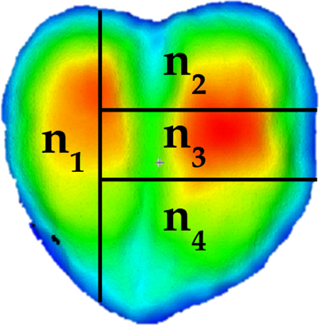
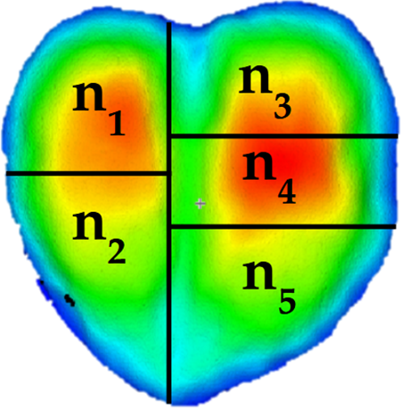
To further address the concern that evaluating only the first segment may underestimate system-wide variability, Gage R&R analyses were extended to include the second and third segments. For the second segment, the total Gage R&R contribution was 8.53%, with repeatability accounting for all the measurement variation. Reproducibility remained at 0.00%, while Part-to-Part variation contributed 99.64%, and the NDC was 16. In the third segment, total Gage R&R accounted for 9.00%, with 7.40% from repeatability and 5.12% from reproducibility (including interaction effects). Part-to-Part variation remained dominant at 99.59%, and the NDC was 15. Detailed results for these segments are presented in Appendix A (Tables A3 and A4).
Real meat portioning test
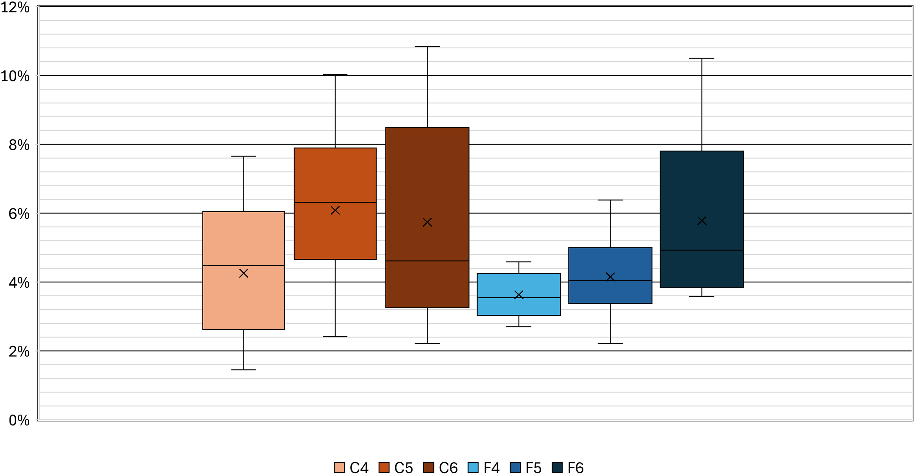
Table 5 and Fig. 15 present the segmentation accuracy for chicken and fish samples across different cutting configurations.
| Pic. | Num of part | Mass (g) | %MAE | SD (g) | Max & Min (%MAE) | |
|---|---|---|---|---|---|---|
| C4 | 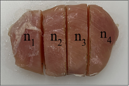 |
4 | 120.5–198.0 | 4.53 | 2.05 | 1.45–7.65 |
| C5 | 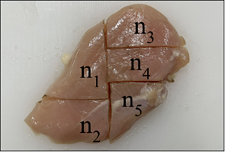 |
5 | 88.1–211.4 | 5.69 | 2.18 | 2.42–8.43 |
| C6 | 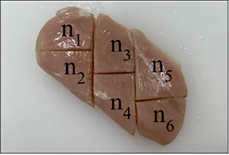 |
6 | 82.9–180.6 | 5.96 | 3.19 | 2.21–10.84 |
| F4 | 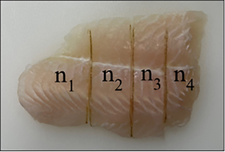 |
4 | 51.8–103.4 | 3.63 | 0.70 | 2.70–4.59 |
| F5 | 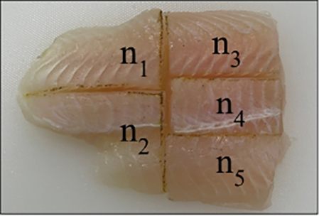 |
5 | 53.9–105.7 | 4.12 | 1.06 | 2.85–5.34 |
| F6 | 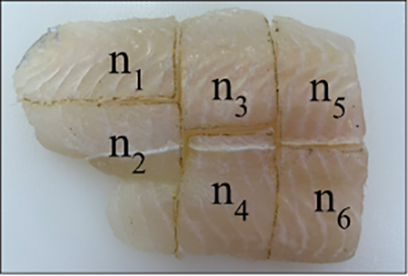 |
6 | 56.9–118.1 | 5.78 | 2.34 | 3.58–10.50 |
Note:
C4, C5, C6 = chicken breast cut into 4, 5, and 6 segments, respectively. F4, F5, F6 = fish fillets cut into 4, 5, and 6 segments, respectively.
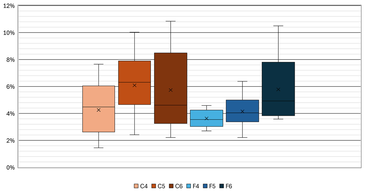
Figure 15: Percentage mean absolute error (%MAE) for chicken breast (C4, C5, C6) and fish fillets (F4, F5, F6) across three cutting configurations: 4, 5, and 6 segments, respectively.
From Table 5, The %MAE values for chicken breast ranged from 4.53% to 5.96%, with standard deviations between 2.05 and 3.19 g. The lowest %MAE for chicken was 1.45% (C4), and the highest was 10.84% (C6). For fish fillets, %MAE ranged from 3.63% to 5.78%, with SD values between 0.70 and 2.34 g. The lowest %MAE for fish was 2.70% (F4), and the highest was 10.50% (F6).
As illustrated in Fig. 15, the %MAE distribution varies between meat types and cutting configurations. Chicken breast groups (C4–C6) generally display higher variability than fish fillet groups (F4–F6), with the widest error ranges observed in the chicken samples with higher segment counts. In contrast, fish fillet groups exhibit narrower interquartile ranges and lower dispersion, indicating more consistent segmentation performance. An increase in the number of segments tends to widen the spread of %MAE for both meat types, though the effect is more pronounced in chicken breast samples.
Discussion
Segmentation errors and limitations in point cloud volume calculation
From Table 1, most deviations are within ±0.5%. While a few segments slightly exceed this margin on the negative side, the overall deviation remains substantially lower than industry standards. For instance, according to the United States Department of Agriculture (USDA) Agricultural Marketing Service (AMS) (United States Department of Agriculture AMS, 2020), portioned meat and poultry products weighing up to 3 oz are allowed a ±10% deviation from the specified weight per unit (this range was selected because it corresponds to the approximate weight of individual pieces after cutting in our experiments).
The last column of Table 1 presents the sum of total segmented volume derived from the calculated cutting lines, which was consistently lower than the total volume computed from the complete point cloud of the object. The cause of the error occurs from the amount of cloud data available. For the algorithm to successfully divide the volume equally, it required a complete point cloud representation of the entire object. Additionally, the number of point cloud data points used in the calculation must be infinitely detailed to ensure that, regardless of the selected cutting position, the volume calculation remained accurate. An example of the volume segmentation limitation is illustrated in Figs. 16A and 16B. If the black dots represent point cloud data points of an object viewed from the above, with a height of one unit. The total volume of the object was calculated by multiplying the green area in Fig. 16A by its height, yielding a volume of 6 units. If the goal was to divide the object into two equal parts, the required volume per segment would have been 6/2 = 3 units. The optimal cutting position was at the center, as shown in Fig. 16B. However, the left-side point cloud data, representing the green area, accounted for only 2 units of volume, while the missing volume corresponded to the red area. As a result, the final portion of the point cloud, which was used for both vertical and horizontal cutting line calculations, lacked sufficient data points to allow adjustments in the cutting position. This limitation prevents the segmented volumes from precisely matching the target volume. In addition to limitations arising from incomplete point cloud data, the current algorithm assumes axis-aligned cuts, which may not be optimal for all organic geometries. While this approach simplifies computation and is suitable for many regular or semi-regular shapes, it imposes a geometric constraint that may not conform well to the complex contours of organic materials such as raw meat.
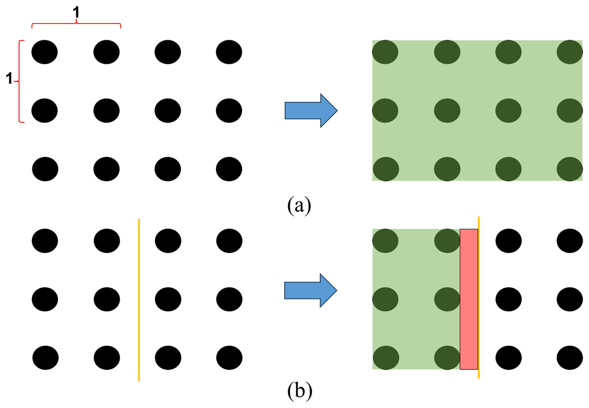
Figure 16: Example of volume segmentation limitations.
(A) Volume calculation from the complete point cloud (green area). (B) Determination of cutting paths using available point cloud data. The red area represents missing data, leading to underestimation of volume in that segment.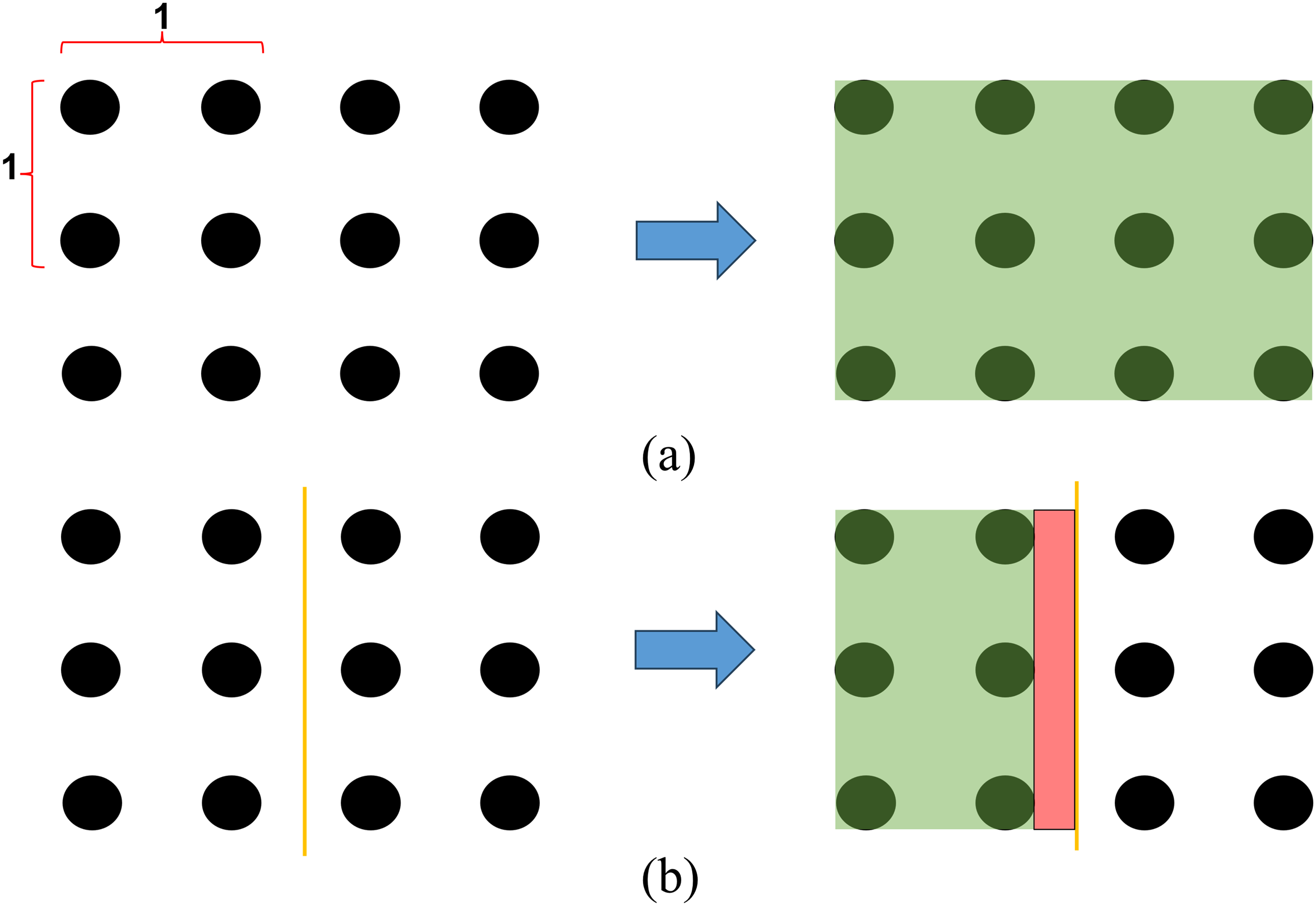
Another factor that may influence the result of clay-based modeling of real meat is the difference in physical properties between modeling clay and biological tissues. Clay provides uniform density and high shape stability, which are advantageous for controlled experiments, but its density, compressibility, and surface compliance differ from those of chicken breast or fish fillets. These differences could affect point cloud acquisition and volume estimation, especially in curved or compliant regions.
Testing different cutting patterns
Table 2 shows that the MAE was 1.8 g, corresponding to a %MAE of 3.54%; the maximum absolute error was 4.4 g, and the maximum percentage error was 8.8%. While 8.8% may appear relatively high, it remains within commonly accepted tolerances in commercial food processing; for example, the USDA Agricultural Marketing Service allows a ±10% deviation for portions up to 3 oz (United States Department of Agriculture AMS, 2020). Evaluating the different cutting patterns in Table 2 further indicates that the proposed algorithm generally achieves equal-weight portions with low %MAE rates. However, some cutting patterns showed higher %Max Error in certain segments. This is partly due to limitations in volume calculation, as discussed in ‘Segmentation Errors and Limitations in Point Cloud Volume Calculation’. Specifically, when point cloud data near the object’s boundaries is sparse or missing, the algorithm has less information to adjust the cutting position precisely to match the target volume. As illustrated in Fig. 16, this issue is more evident in patterns with fewer or larger segments, where boundary errors have a greater impact. Additionally, the physical shape of the object may also affect the segmentation accuracy. Irregular or curved surfaces can cause under or overestimation of volume in specific areas, particularly when cuts intersect regions with varying thickness.
The results of the One-Way ANOVA test revealed significant differences in MAE across various cutting patterns, confirming that the choice of pattern had a substantial impact on segmentation accuracy. These findings suggested that while the algorithm was effective in portioning, further optimization of the cutting algorithm is necessary to improve weight distribution consistency and minimize errors in portioning systems.
Gage R&R
As reported in the Results section, these results verify that the measurement system contributes minimally to the observed variability, and that most differences in portion weight arise from the samples themselves rather than measurement error, supporting the system’s suitability for industrial use. The small reproducibility component detected only in the third segment is consistent with its spatial location near object boundaries in several cutting patterns, where geometry changes more rapidly and the field of view of the laser line profile sensor can be marginal. Because only the upper surface is captured, slight placement differences can yield incomplete or distorted point clouds at the edges, introducing small but detectable deviations in volume estimation and producing the observed Operator × Part interaction. Despite this sensitivity, the total Gage R&R for the third segment remained below 10%, and Part-to-Part variance still dominated, confirming robust discrimination across weight levels and overall reliability of the system.
Testing chicken breast and fish portioning
The expanded real meat evaluation confirmed that the developed cutting algorithm maintained acceptable segmentation accuracy for both chicken and fish under realistic processing conditions. In chicken breast samples, most of %MAE values remained within the USDA Agricultural Marketing Service standard (United States Department of Agriculture AMS, 2020), which permits ±10% weight variation for individual meat or poultry portions weighing up to 3 oz, although variability increased slightly with higher segment counts. This trend suggests that when the number of cuts increases, the cumulative effect of small volumetric estimation errors becomes more pronounced.
In contrast, fish fillets demonstrated lower %MAE values and smaller variability ranges across comparable segment counts. This performance difference is likely due to the flatter and more uniform morphology of fish fillets, which facilitates more complete point cloud acquisition and more accurate volume estimation. These characteristics reduce the impact of surface irregularities that are more prominent in chicken breasts, such as variable thickness and muscle curvature. The increase in %MAE for F6 compared to F4 and F5 indicates that even for more uniform products, segmentation into a higher number of pieces can introduce additional errors. Furthermore, previous research has suggested that an error margin of around 8% is considered acceptable in the field (Jang & Seo, 2023), and for fish cutting, the %MAE observed here was consistently below this threshold in most configurations.
Overall, the findings support the robustness of the proposed system in producing weight-consistent portions for irregularly shaped raw meat products, while highlighting the importance of optimizing point cloud density and segmentation algorithms, particularly for products with complex surface geometries, to maintain accuracy at higher cut counts.
Conclusions
This research developed a vision based cutting algorithm to enhance precision in meat portioning by ensuring equal-weight distribution. The proposed system employed a laser line profile sensor to capture point cloud data, which was processed to generate optimal cutting lines. The algorithm was validated through rigorous testing, including MAE, One-Way ANOVA, and Gage R&R analysis, demonstrating high segmentation accuracy and repeatability.
Experimental results confirmed that the system effectively minimized segmentation errors and maintained consistency in portion sizes, meeting industry standards for food processing. Testing with both modeling clay and real meat samples verified the robustness of the algorithm in handling shape and density variations. The low variability observed in Gage R&R analysis underscored the reliability and repeatability of the measurement system.
Despite its effectiveness, some challenges remain, including the impact of natural irregularities in meat texture and density on segmentation accuracy. Future improvements should focus on enhancing real-time adaptability and integrating deep learning models to improve decision-making based on variations in sample properties, such as thickness or internal density. For instance, learning from 3D point cloud patterns could help predict segmentation errors and adjust cutting lines accordingly. Moreover, the system could be extended to other food sectors beyond meat, such as dairy or bakery products, where volume-based segmentation and precision cutting are also beneficial, thereby demonstrating the scalability of the proposed approach.
Overall, this study advances automated meat portioning technology by reducing reliance on manual labor, minimizing material waste, and improving processing efficiency, contributing to more sustainable and precise food production.