From prediction to trust: enhancing deep learning models for insurance fraud detection through uncertainty quantification

Ziad Salem; Samer Sahl; Mohamed Hanafy Kotb Ibrahim

doi:10.7717/peerj-cs.3365

From prediction to trust: enhancing deep learning models for insurance fraud detection through uncertainty quantification

Ziad Salem ¹, Samer Sahl², Mohamed Hanafy Kotb Ibrahim ^2,3

1School of Economics & Management, Qujing Normal University, Qujing, Yunnan, China

2Department of Statistics, Mathematics, and Insurance, Faculty of Commerce, Assiut University, Assiut, Assiut, Egypt

3School of Risk & Actuarial Studies, University of New South Wales, South Wales, New South Wales, Australia

DOI: 10.7717/peerj-cs.3365

Published: 2025-12-04
Accepted: 2025-10-15
Received: 2025-06-02

Academic Editor: Xiangjie Kong

Subject Areas: Algorithms and Analysis of Algorithms, Artificial Intelligence, Data Mining and Machine Learning, Data Science
Keywords: Insurance fraud detection, Deep learning, Uncertainty quantification, SHAP values, Resampling

Copyright: © 2025 Salem et al.
Licence: This is an open access article distributed under the terms of the Creative Commons Attribution License, which permits unrestricted use, distribution, reproduction and adaptation in any medium and for any purpose provided that it is properly attributed. For attribution, the original author(s), title, publication source (PeerJ Computer Science) and either DOI or URL of the article must be cited.

Cite this article: Salem Z, Sahl S, Ibrahim MHK. 2025. From prediction to trust: enhancing deep learning models for insurance fraud detection through uncertainty quantification. PeerJ Computer Science 11:e3365 https://doi.org/10.7717/peerj-cs.3365

The authors have chosen to make the review history of this article public.

Abstract

This study applies uncertainty quantification techniques to deep neural networks for automobile insurance fraud detection to address the critical need for confidence estimation in artificial intelligence (AI)-driven decision systems. We evaluate three uncertainty quantification approaches: Monte Carlo Dropout (MCD), Deep Ensembles, and Ensemble Monte Carlo Dropout (EMCD) on a dataset of 15,420 insurance claims. Our framework incorporates SHapley Additive exPlanations (SHAP) based interpretability analysis and introduces uncertainty-specific evaluation metrics through an uncertainty confusion matrix. We examine how data resampling techniques (Random Over-Sampling (ROS) and Synthetic Minority Oversampling Technique (SMOTE)) affect both predictive performance and uncertainty calibration. Results demonstrate that while resampling improves fraud detection sensitivity, it increases predictive uncertainty by 65.12% to 298.55%. Critically, this increased uncertainty strongly correlates with model misclassifications, indicating improved self-awareness of prediction reliability. The EMCD approach achieves the highest fraud detection rates but with elevated uncertainty, while ensemble methods provide more conservative predictions with better calibration. These findings contribute to developing trustworthy AI systems for insurance fraud detection by providing both predictions and associated confidence measures.

Introduction

The insurance industry loses billions annually due to fraudulent activities, as highlighted by reports from the Association of British Insurers (2021) and European Insurance Federation (2019). Such losses impact not only companies but also escalate costs for honest policyholders through increased premiums (Viaene et al., 2007). Detecting fraud not only results in significant savings but also reinforces the integrity of the market, acting as a strong deterrent against malpractices (Picard, 1996; Tennyson & Salsas-Forn, 2002). In the vast realm of insurance, automobile fraud detection emerges as a particular challenge, emphasizing the need for innovative solutions. With the evolving tactics of fraudsters, the industry requires sophisticated and transparent methods. This is where artificial intelligence (AI) comes into the picture. With its potential for detecting intricate patterns within vast datasets, AI is poised as a promising tool to address the challenge of insurance fraud detection, especially in the automobile sector.

Machine learning, notably through deep networks, has been instrumental in bridging the gap between human expertise and computational prowess. These networks have demonstrated unmatched competencies in predictive analytics, data interpretation, and visualization across domains (Thomas et al., 2019; Wu, Wang & Zhang, 2019). This ascent has been fuelled by state-of-the-art computational resources, large-scale datasets, and the continuous evolution of deep learning methodologies (Lecun, Bengio & Hinton, 2015).

While the majority of previous research has focused on supervised and unsupervised learning tools, from logistic regressions to artificial neural networks (Caudill, Ayuso & Guillén, 2005; Gomes, Jin & Yang, 2021; Viaene et al., 2002; Wang & Xu, 2018), there remains an unexplored area: the uncertainty in Deep Neural Networks (DNNs) when detecting insurance fraud. DNNs, often termed as “black box” models, face criticism due to their lack of transparency. Their intricate architectures, though powerful, make their decision-making processes enigmatic (Samek, Wiegand & Müller, 2017). This opacity is a hurdle in sectors like insurance where understanding and trust are paramount.

In this study, we address the challenge of understanding and quantifying the uncertainty associated with AI in the detection of insurance fraud, specifically in the context of DNNs. Our research is driven by the need for transparency and reliability in AI applications within the insurance sector, a field where the accuracy and trustworthiness of predictions are crucial.

Our work focuses on Uncertainty Quantification (UQ) techniques. These techniques not only provide results but also offer a measure of confidence in these results. This dual approach is essential for building trust and understanding the reliability of AI predictions in insurance fraud detection.

The contributions of our research are multifaceted and significant in addressing the complex challenges in the insurance sector:

(1)

Advanced uncertainty techniques: This article leverages and adapts existing techniques for managing uncertainty, including Monte Carlo Dropout (MCD), ensemble methodologies, and Ensemble Monte Carlo Dropout (EMCD), for automobile insurance data. These techniques, previously applied in fields such as medical imaging classification (Abdar et al., 2021; Asgharnezhad et al., 2022; Zeevi et al., 2024), are evaluated in the context of insurance to demonstrate their applicability and effectiveness in this domain.
(2)

Impact of dataset rebalancing: We explore the effects of dataset rebalancing strategies, such as Random Over-Sampling (ROS) and Synthetic Minority Oversampling Technique (SMOTE), especially focusing on how they influence uncertainty quantification.
(3)

Enhancing interpretability: We integrate SHapley Additive exPlanations (SHAP) values to unravel the decision-making processes of DNNs, thereby enhancing the interpretability and understanding of these models.
(4)

Rigorous evaluation: Our research employs a unique combination of the UQ confusion matrix and the conventional confusion matrix. This dual-matrix approach allows for a more profound insight into the predictive uncertainties and provides a thorough statistical evaluation.

Our overarching goal is to bridge the gap between the complex capabilities of DNNs and the need for transparency in the insurance industry. We aim to advance the field of automobile insurance fraud detection by providing a comprehensive, reliable, and transparent framework for using AI. This research goes beyond simple prediction; it emphasizes understanding and quantifying the reliability and uncertainty of AI predictions. Through detailed analyses and comprehensive documentation, we present a new paradigm in leveraging AI for the detection of automobile insurance fraud, characterized by credibility and transparency.

This article is structured as follows: “Literature Review” provides an extensive review of literature on insurance fraud detection. In “SHapley Additive exPlanations”, we thoroughly examine UQ approaches, with special emphasis on the UQ confusion matrix and the principles of SHAP. “Materials and Methods” details the dataset used and outlines our experimental methodology. Our results and their implications are presented in “Results”. Finally, “Conclusion” concludes the study and suggests potential areas for future research.

Literature review

Insurance fraud detection, a critical challenge across various domains, has witnessed significant academic exploration over the years. As the sector grapples with the evolving tactics of fraudsters, it simultaneously sees rapid advancements in technology and analytics. Researchers worldwide have delved into multiple avenues to enhance fraud detection, particularly focusing on the potential of data science, machine learning, and deep learning. This literature review provides a comprehensive synthesis of these research endeavors. This review captures the landscape of fraud detection methods. Through this exploration, we aim to present the current state of research and highlight gaps and opportunities for further investigation.

Johnson & Khoshgoftaar (2019) delved into the issue of prevalent fraud in U.S. Medicare. They utilized Medicare claims data to tackle the class-imbalance problem in fraud detection, assessing six deep learning techniques. They particularly focused on data-level strategies such as ROS, random under-sampling (RUS), and a hybrid approach combining both.

In a study by Zhang, Xiao & Wu (2020), a neural network model incorporating fully connected layers and sparse convolution was proposed to assess the relationship between diseases and drugs. The study aimed to detect anomalies based on a quantified relationship score and additional features, such as a relative probability score, to measure the model’s performance. By addressing data imbalance through a focal-loss function, the model demonstrated improved anomaly detection in medical data. This approach is relevant to fraud detection in insurance, as similar methodologies can be applied to identify anomalous patterns and behaviors indicative of fraudulent activities in large, complex datasets.

Herland, Bauder & Khoshgoftaar (2019) investigated the U.S. healthcare system, emphasizing the detection challenges stemming from the imbalance between genuine and fraudulent transactions. By analyzing Medicare ‘Big Data’ claims datasets, the study found a decline in fraud detection efficacy where fraudulent activities were less frequent. Various methods, including random under-sampling, were conducted. The research concluded that a training and testing approach was more efficacious than Cross-Validation in pinpointing Medicare fraud.

Sun et al. (2019) discussed the difficulties of detecting joint fraud in the medical sector, characterized by its rarity and fraudsters’ deceptive strategies. Traditional approaches frequently misclassify individuals with uncommon behaviors as fraudulent, leading to elevated false positives. To mitigate this, the researchers introduced an “abnormal group-based joint fraud detection method.” Using person similarity adjacency graphs, this method improved fraud detection accuracy by over 10%, substantially diminishing false positives.

Ekin, Lakomski & Musal (2019) proposed an unsupervised Bayesian hierarchical technique aimed at aiding initial medical fraud assessments. By grouping medical procedures and revealing hidden patterns among providers, the method provides valuable insights for medical audit decisions through outlier detection and similarity evaluations.

Nalluri et al. (2023) emphasized that while numerous studies have addressed medical insurance fraud, few have explored its core determinants. In this investigation, two distinct datasets were analyzed using four machine learning techniques: support vector machine (SVM), decision tree (DT), Random Forest (RF), and multilayer perceptron (MLP). The research aimed not only to determine the optimal detection method but also to identify 19 crucial features of medical insurance fraud.

Óskarsdóttir et al. (2022) approached insurance fraud detection by adopting social network analysis. By linking claims with all pertinent parties, a holistic network was established. Leveraging the BiRank algorithm, each claim was assigned a fraud score, enhancing motor insurance fraud detection through the amalgamation of network-derived features and specific claim details.

Wang & Xu (2018) introduced a novel method for automobile insurance fraud detection by combining LDA for text analysis with deep neural networks. By analyzing text data from accident descriptions, this method outperformed conventional models on real-world datasets, underscoring its potential for fraud detection.

Gomes, Jin & Yang (2021) detailed a deep learning technique tailored to understand insured individual behavior through unsupervised variable significance. By merging autoencoder and variational autoencoder models, the research accentuated the importance of qualitative evaluation methods in conjunction with quantitative metrics.

Stripling et al. (2018) put forth iForestCAD, an innovative method that augments insurance fraud detection by providing conditional anomaly scores. This technique was trialed on real workers’ compensation claims and was proven effective.

Debener, Heinke & Kriebel (2023) explored both supervised and unsupervised learning for insurance fraud detection. Although supervised learning has been extensively studied, the research accentuated the untapped potential of unsupervised methods, such as isolation forests. Both strategies were deemed promising, with the research recommending their combined use for exhaustive detection.

Yan et al. (2020) highlighted the growing challenge of insurance fraud in the expanding insurance sector. This study introduced a unique method, merging an improved adaptive genetic algorithm (NAGA) with a backpropagation (BP) neural network. By optimizing the BP neural network’s initial weight, limitations like the risk of local minima and sluggish convergence were addressed. With historical automobile insurance claim data, the NAGA-BP model showcased enhanced prediction accuracy and swifter convergence relative to traditional techniques.

Sowah et al. (2019) addressed the critical issue of health insurance fraud, which hinders service delivery and induces financial losses. Analyzing data from Ghana’s National Health Insurance Scheme, the study introduced the Genetic Support Vector Machines (GSVMs) as a tool for fraud detection. The experiments demonstrated that GSVMs, especially when using the radial basis function kernel, offer efficient and accurate fraud detection capabilities.

Hancock & Khoshgoftaar (2021) studied the effectiveness of various algorithms for detecting Medicare fraud using claims data. A focal point of their research was the impact of incorporating categorical features. Their findings accentuated the superior performance of the categorical boosting (CatBoost) algorithm over the Light Gradient-Boosting Machine (LightGBM). Notably, when an additional categorical feature was integrated into the model, CatBoost’s performance experienced a marked improvement. Such findings underscore CatBoost’s potential as an invaluable tool for detecting fraud, especially in Medicare datasets containing categorical variables.

These works highlight the ever-evolving nature of techniques being used in fraud detection and underscore the need for innovative approaches to meet the dynamic challenges of the sector. An overview of these studies can be found in Table 1.

Table 1:

Overview of contemporary research in insurance fraud detection.

Study	Domain	Data modality	Learning paradigm	Imbalance handling	SHAP	Uncertainty/calibration	Key strength/limitation
Stripling et al. (2018)	workers’ compensation	Tabular	Supervised and Unsupervised	Weights inversely	N/A	N/A	Practical anomaly scoring; calibration unclear
Wang & Xu (2018)	Automobile	Text + Tabular	Supervised and Unsupervised	SMOTE	N/A	N/A	Text augments detection; UQ absent
Johnson & Khoshgoftaar (2019)	Health	Tabular	Supervised	ROS/RUS/Hybrid	N/A	N/A	Strong deep baseline; limited UQ/calibration
Herland, Bauder & Khoshgoftaar (2019)	Health	Tabular	Supervised	RUS	N/A	N/A	Highlights protocol sensitivity; lacks UQ
Sun et al. (2019)	Health	Tabular	Supervised and Unsupervised	N/A	N/A	N/A	Cuts false positives;thresholding still needed
Ekin, Lakomski & Musal (2019)	Health	Tabular	Unsupervised	N/A	N/A	N/A	Label-lean discovery; thresholding challenge
Sowah et al. (2019)	Health	Tabular	Supervised	N/A	N/A	N/A	Accurate detection; thresholds/costs unclear
Yan et al. (2020)	Automobile	Tabular	Supervised	N/A	N/A	N/A	Optimization gains; no calibrated risk
Zhang, Xiao & Wu (2020)	Health	Tabular	Supervised and Unsupervised	Focal loss	N/A	N/A	Strong imbalance remedy; UQ not studied
Hancock & Khoshgoftaar (2021)	Health	Tabular	Supervised	RUS	N/A	N/A	CatBoost advantages; calibration not covered
Gomes, Jin & Yang (2021)	Automobile	Tabular	Supervised and Unsupervised	N/A	N/A	N/A	Finds latent structure; probability calibration not covered
Hanafy & Ming (2021)	Automobile	Tabular	Supervised	ROS/RUS/SMOTE	N/A	N/A	Early study on class imbalance; calibration and uncertainty were not assessed
Óskarsdóttir et al. (2022)	Automobile	Tabular	Supervised and Unsupervised	SMOTE	N/A	N/A	Network context boosts accuracy; calibration open
Debener, Heinke & Kriebel (2023)	Automobile	Tabular	Supervised and Unsupervised	N/A	Feature Importance	N/A	Argues hybrid detection; UQ gap remains
Nalluri et al. (2023)	Health	Tabular	Supervised	N/A	N/A	N/A	Identifies important features; UQ absent
Maiano et al. (2023)	Automobile	Images	Supervised	N/A	N/A	N/A	End-to-end computer-vision antifraud system; little on calibration/UQ
Alharbi, Al-Faries & Alabdulkarim (2023)	Health	Tabular	Supervised	SMOTE	N/A	N/A	Regional real-world study; classic supervised stack; lacks calibration
Vorobyev (2024)	Automobile	Tabular	Supervised and Unsupervised	Rule Induction	N/A	N/A	Graph connectivity boosts PR-AUC; lacks calibration/UQ
Deprez et al. (2024)	Automobile & Health	Tabular	Supervised	Gradient boosting classifier	N/A	NA	Practical comparison; network features add distinct signal
du Preez et al. (2025)	Health	Tabular	Supervised and Unsupervised	ROS/RUS/SMOTE/ADASYN	N/A	N/A	State-of-the-art synthesis; gaps in calibration/UQ and label scarcity
Ming et al. (2024a)	Automobile	Tabular	Supervised	ROS/RUS	Varies	N/A	Practical ensemble baselines; no UQ metrics
Ming et al. (2024b)	Automobile & credit cards	Tabular	Supervised	ROS	N/A	N/A	Simple, practical hybrid; no UQ/calibration reported
Yankol-Schalck (2025)	Automobile	Tabular	Supervised	Cost-sensitive learning	Varies	N/A	Pushes cost-aware training at intake; still lacks UQ metrics
Anand Kumar & Sountharrajan (2025)	Automobile	Images	Supervised	N/A	N/A	N/A	DL with hyperparameter optimization; needs calibration & external validation

DOI: 10.7717/peerj-cs.3365/table-1

Unlike prior fraud-detection studies that report discrimination metrics alone, we evaluate whether models are reliably confident, using an uncertainty-aware confusion matrix and calibration analyses, and we quantify how class rebalancing reshapes both accuracy and uncertainty. Reliable predictive modeling hinges on UQ, which addresses two principal sources of uncertainty: epistemic uncertainty, arising from limited data and model specification choices (e.g., architecture, parameterization, and hyperparameters), and aleatoric uncertainty, which is inherent in the data and irreducible (Gawlikowski et al., 2023; Der Kiureghian & Ditlevsen, 2009). An ideal system accurately quantifies aleatoric uncertainty while minimizing epistemic uncertainty through improved learning and design choices. In practice, however, deep models make UQ challenging, as design decisions regarding model class, depth, width, regularization strategies, and learning rates introduce additional layers of uncertainty. For high-stakes applications such as medical diagnosis and fraud detection, average accuracy metrics are insufficient; practitioners require calibrated, instance-level confidence estimates to support sound risk assessment and decision-making (Amodei et al., 2016). This critical need has driven the development of a diverse toolbox of UQ methods, including deep ensembles that aggregate predictions from multiple independently trained models (Lakshminarayanan, Pritzel & Blundell, 2017), Monte Carlo Dropout which leverages stochastic regularization during inference (Gal & Ghahramani, 2016). However, evaluating the quality of uncertainty estimates presents significant methodological challenges. Standard population-level metrics such as accuracy provide aggregate performance summaries but fail to capture whether uncertainty estimates are well-calibrated at the individual prediction level. This evaluation gap becomes particularly concerning for fraud detection applications, where practitioners need reliable confidence indicators to prioritize manual investigations, manage false alarm rates, and make informed decisions about resource allocation. While recent work in financial fraud detection has begun addressing these challenges through specialized evaluation frameworks (Habibpour et al., 2023), the application of uncertainty quantification to insurance fraud detection remains underexplored despite the domain’s clear operational need for trustworthy, confidence-aware prediction.

As Table 1 shows prior work delivers strong detectors across tabular, text, and network settings, and routinely applies rebalancing to address class imbalance. Yet two practice-critical elements remain underdeveloped: (i) predictive uncertainty and calibration, whether models are reliably confident, and (ii) how rebalancing alters uncertainty, especially on errors. Our study addresses both by comparing MCD, Deep Ensembles, and EMCD, using an uncertainty-aware confusion matrix, and showing that resampling systematically changes both accuracy and confidence, with the largest uncertainty increases concentrated on misclassified claims.

Materials and methods

In this section, we examined three uncertainty-quantification approaches for neural networks, MCD, deep ensembles and EMCD, using the original imbalanced claims-fraud dataset together with two re-balanced variants produced via ROS and SMOTE. For every model–dataset combination we computed standard diagnostic measures (accuracy, sensitivity, specificity) alongside the uncertainty-oriented counterparts derived from the Uncertainty Confusion Matrix (uncertainty-accuracy, uncertainty-sensitivity, uncertainty-specificity, uncertainty-precision), selecting the classification cut-off that minimized the spread among accuracy, sensitivity and specificity. Validation employed a single stratified 70/30 train–test split that preserved the fraud prevalence; all resampling and hyper-parameter tuning were confined to the training subset to prevent information leakage, and final performance was recorded once on the untouched test subset. Taken together, this hold-out design and threshold-sweep constitute the evaluation method, while the reported diagnostic and uncertainty figures are the metrics that summarize its outcomes. To demonstrate the robustness of the proposed uncertainty-aware fraud-detection framework, we adopted a three-step evaluation protocol that focuses on how the models were validated see Table 2.

Table 2:

Evaluation protocol for the uncertainty-aware fraud-detection framework, summarizing each validation step’s purpose, and procedure.

Step	Purpose	Procedure
1. Stratified hold-out validation	Obtain an unbiased estimate of generalisation performance.	The dataset was split once into 70% training and 30% test sets with stratification on the fraud label so that the 6% fraud prevalence was preserved. All data transformations (standard-scaling, ordinal encoding), resampling operations (ROS or SMOTE), and hyper-parameter searches were performed exclusively on the training partition. The untouched test set was consulted only once, after model fitting, to compute final performance and uncertainty statistics.
2. Ablation study	Isolate the influence of (a) the uncertainty-quantification technique and (b) the class-balancing strategy.	nine candidate pipelines were trained: • Original + MCD • Original + Ensemble • Original + EMCD • ROS + MCD • ROS + Ensemble • ROS + EMCD and the same triplet with SMOTE. Comparing these pipelines constitutes an ablation experiment that quantifies how each modelling choice alters both accuracy-based and uncertainty-based behaviour.
3. Threshold calibration sweep	Select an operating point that balances false-positive and false-negative costs.	For every trained model the posterior fraud probability on the test set was converted to a binary decision by sweeping the classification thresholds. At each cut-off we computed accuracy, sensitivity and specificity; the threshold that minimised the sample variance of these three quantities was chosen as the balanced operating point and was used in all downstream comparisons, including the uncertainty-confusion-matrix analysis.

DOI: 10.7717/peerj-cs.3365/table-2

Monte-Carlo dropout (MCD)

MCD, presents an innovative approach to neural networks (Gal & Ghahramani, 2016). Traditional dropout, which is primarily used during training, is extended into the evaluation phase with MCD. This technique treats output samples as Monte Carlo samples. These samples are procured by leveraging regular dropout within DNN during the testing phase. To apply the MCD approach, there are certain prerequisites. Firstly, the DNN should be initially trained with dropout. Once this is achieved, for each input inference, the DNN must be executed T times, but with dropout incorporated during the evaluation. Crucially, while the input remains consistent across these iterations, a different, randomly generated dropout mask is applied during each pass.

The estimators for both mean and variance of model outputs can be articulated as:

$E [y | x] \approx \frac{1}{T} \sum_{i = 1}^{T} {\hat{y}}_{i} (x),$

$V a r E [y | x] \approx \frac{1}{T} \sum_{i = 1}^{T} {\hat{y}}_{i} (x)^{T} y_{i} (x)^{⊤} - E [y | x] E [y | x]^{⊤} + τ^{- 1} I_{D},$ where:

${\hat{y}}_{i} (x)$ is the prediction from the i-th forward pass for input x,
T is the total number of forward passes,
is a regularization term linked to the dropout rate, and
$I_{D}$ is the identity matrix of size D, the output dimension.

The term $τ^{- 1} I_{D}$ accounts for model uncertainty due to weight regularization. The predictive distribution for a network with input $x$ and output $y$ , trained on a dataset

$D_{t r a i n}$ with $L$ layers and parameters represented by $w$ . The predictive distribution can be denoted as:

$p (y ∣ x, D_{t r a i n}) = \int p (y ∣ x, w) p (w ∣ D_{t r a i n}) d w$ where:

$p (y ∣ x, w)$ represents the model’s likelihood,

$p (w ∣ D_{t r a i n})$ stands for the posterior weight distribution.

As elaborated by Gal & Ghahramani (2016), this posterior, computationally challenging to determine, can be approximated as $q (w)$ . Through variational techniques, this distribution transforms to:

$q (y ∣ x) = \int p (y ∣ x, w) q (w) d w$

Gal & Ghahramani (2016) have indicated that the chosen approximated posterior, $q (w)$ , mirrors a distribution of the weight matrix but with randomly dropped connections. Realized by incorporating dropout during testing, $q (w)$ can be given as:

$W_{i} = M_{i} \times d i a g ({[z_{i, j}]}_{j = 1}^{K_{i}}),$ where $z_{i, j}$ are Bernoulli random variables and $M_{i}$ represents the learned weights for layer $i$ .

By sampling $T$ dropout masks, a set ${W_{1}^{t}, \dots, W_{L}^{t}}_{t = 1}^{T}$ is established. This aids in simplifying the predictive mean for a given input:

$E_{q (y ∣ x) (y)} \approx \frac{1}{T} \sum_{t = 1}^{T} \hat{y} (x, W_{1}^{t}, \dots, W_{L}^{t})$

Deep ensemble

Deep Ensemble serves as an aggregation of deep learning models, each bearing unique weight initializations. When multiple models, each with their distinct weight setups, are trained, they inevitably produce varied outputs for any given prediction. This variation resembles the multiplicity seen in MCD, but with a key distinction: each model in the ensemble operates with wholly independent parameters (Filos et al., 2019).

The resulting predictive mean can be represented as:

$\hat{y} = p_{e n s e m b l e} (y = c ∣ x) = \frac{1}{T} \sum_{i = 1}^{T} M_{i} (x),$ where $p_{e n s e m b l e} (y = c x)$ : The probability that the input $x$ belongs to class $c$ , estimated by the ensemble. $M_{i} (x)$ : signifies the prediction yielded by the $i^{t h}$ model, $M_{i}$ , for a specified input $x$ .

Ensemble Monte Carlo dropout (EMCD)

EMCD is an ensemble of MC-Dropout networks; predictions average over both ensemble members and dropout samples, combining parameter diversity with stochastic inference.

$E [y | x] \approx \frac{1}{M T} \sum_{m = 1}^{M} \sum_{t = 1}^{T} {\hat{y}}_{m, t} (x),$

The EMCD Dropout approach combines multiple MCD models, operating them concurrently. In this method, continuous sampling occurs across all ensemble members. Each of these individual models mandates the application of distinct dropout masks for every sample. Upon computing the estimates from each model, they are collectively averaged to derive the final EMC outcome. Importantly, the EMCD integrates two pivotal UQ techniques: MCD and Model Ensembling.

Uncertainty confusion matrix

Drawing inspiration from the traditional confusion matrix, we introduce a set of quantitative metrics tailored for predictive uncertainty estimates. We initiate our approach by juxtaposing predictions against ground truth labels, categorizing them as either ‘True’ or ‘False’. Similarly, based on a predetermined threshold, predictive uncertainty estimates are classified as ‘certain’ or ‘uncertain’ (Asgharnezhad et al., 2022).

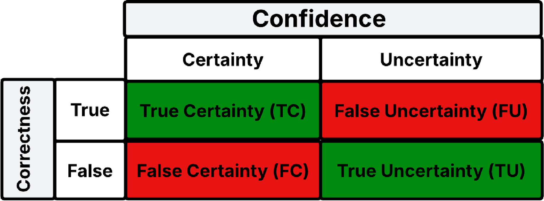
When these classifications are cross-referenced, they yield four distinct outcomes, illustrated in Fig. 1:

Correct predictions that are certain, termed as True Certainty (TC).
Incorrect predictions that are uncertain, denoted as True Uncertainty (TU).
Correct predictions that are uncertain, labeled as False Uncertainty (FU).
Incorrect predictions that are certain, designated as False Certainty (FC).

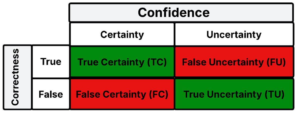
Figure 1: Uncertainty confusion matrix.

Download full-size image

DOI: 10.7717/peerj-cs.3365/fig-1

It is noteworthy that TC and TU represent the ideal scenarios, analogous to the TN and TP in a standard confusion matrix. While FU can be viewed in a positive light (given the prediction, though uncertain, is accurate), FC is particularly concerning, it signifies an erroneous prediction made with confidence by the model. Based on these definitions, we adapt the metrics introduced by Asgharnezhad et al. (2022) to evaluate predictive uncertainty estimates in the context of automobile insurance data.

Uncertainty sensitivity (USen): This is calculated as the number of incorrect and uncertain predictions (TU) divided by the total number of incorrect predictions:

$U S e n = \frac{T U}{T U + F C} .$

USen, sometimes termed Uncertainty Recall, mirrors the sensitivity (recall) or True Positive Rate from the conventional confusion matrix. It holds vital significance as it quantifies the model’s ability to convey its confidence in misclassified samples.

Uncertainty specificity (USpe): USpe is derived by taking the number of correct and certain predictions (TC) and dividing it by the total number of correct predictions:

$U S p e = \frac{T C}{T C + F U} .$

USpe, or the Correct Certain Ratio, parallels the specificity metric in traditional contexts.

Uncertainty precision (UPre): UPre is computed as the number of incorrect and uncertain predictions (TU) divided by the total number of uncertain predictions:

$U P r e = \frac{T U}{T U + F U} .$

UPre aligns with the concept of precision in traditional binary classification.

Uncertainty accuracy (UAcc): Analogous to accuracy metrics for classifiers, UAcc measures the proportion of all diagonal outcomes to the total outcomes:

$U A c c = \frac{T U + T C}{T U + T C + F U + F C} .$

Optimal USen, USpe, UPre, and UAcc values are one, while the least favorable are zero. Ideally, these metrics should be as close to one as feasible. High values for USen, USpe, and UPre signify a network that is self-aware, discerning its knowns and unknowns. Such a network can provide guidance on the trustworthiness of its predictions, accurately gaging and communicating its confidence level.

SHapley Additive exPlanations (SHAP)

A leading approach to clarifying predictions made by machine learning models is the SHAP technique. Pioneered by Lundberg, Allen & Lee (2017), SHAP provides a framework for interpreting a machine learning model, grounding its principles in the additive feature attribution method. Explainable Artificial Intelligence (XAI) seeks to illuminate the decision-making processes of machine learning (ML) models. In essence, XAI strives to clarify the significance of different factors in influencing predictions, providing analysts with insights into the reasoning behind the model’s determinations, particularly in areas such as insurance.

XAI techniques can be categorized into two primary types: global and local explanations. Global methodologies present an overarching view, elucidating the primary factors and their averaged impact on model predictions.

On the other hand, local explanations dive deeper into individual predictions. They aim to elucidate which specific factors play a dominant role in each distinct prediction.

Let’s consider an input model defined through a linear combination of input variables. If the model’s input variable is denoted as $x$ , and the original model is represented by $f (x)$ , then the interpretation model $g (x^{'})$ for the simplified input $x^{'}$ can be articulated as:

$f (x) = g (x^{'}) = ϕ_{0} + \sum_{i = 1}^{M} ϕ_{i} x_{i}^{'}$

Here, $M$ signifies the count of input features. The term $ϕ_{0}$ serves as a constant value in scenarios where all features are absent.

Each SHAP value, $ϕ_{i} (f, x)$ , quantifies the influence of the $i^{t h}$ feature on the model prediction $f$ for a given input $x$ . The term $F$ refers to the complete set of features, with $S$ being its subset. Note that $S \subseteq F / {i}$ includes all feature subsets that incorporate the $i^{t h}$ feature. The cardinalities of $F$ and $S$ are represented by $| F |$ and $| S |$ , respectively. For assessing the significance of each feature, two models are trained: one (i.e., $f_{S \cup {i}}$ ) with the specific feature available and another (i.e., $f_{S}$ ) without that feature (Kim & Kim, 2022). The input subset containing only the features in $S$ is given by $x_{S}$ . The mean SHAP value is computed based on the average absolute SHAP value for each feature, as depicted:

$ϕ_{i} (f, x) = \sum_{S \subseteq F / {i}} \frac{| S |! (| F | - | S | - 1)!}{| F |!} [f_{S \cup {i}} (x_{S \cup {i}}) - f_{S} (x_{S})] .$

Dataset

The dataset, sourced from Oracle, addresses the pivotal matter of insurance fraud detection within the auto insurance sector. Spanning two years, it documents 15,420 auto insurance claims made in the U.S. Of these claims, 923 were marked as fraudulent, while 14,497 were recognized as legitimate (Ming et al., 2024b, 2024a).

In its original state, the dataset encompassed 33 features. However, for the purpose of streamlined analysis, non-essential variables, including identification metrics and overlapping information, were omitted. Consequently, the curated dataset, made available by Datawatch Angoss, comprises select variables which are elucidated in Table 3. Preprocessing followed standard practice: numeric predictors were z-score standardized, ordered categorical variables were ordinal-encoded, and nominal categoricals were one-hot encoded, with all transformations fit on the training data only to avoid leakage.

Table 3:

Data set features.

Month	Sex	Driver rating
Week of month	Marital status	Days policy accident
Day of week	Age	Days policy claim
Make	Fault	Past number of claims
Accident area	Address change claim	Age of vehicle
Month of claim	Vehicle category	Base policy
Week of month claim	Vehicle price	Police report filed
Day of week claim	Deductible	Witness present
Number of suppliments	Number of cars	Fraud found
Agent type	Policy type

DOI: 10.7717/peerj-cs.3365/table-3

In our research, we undertook rigorous pre-processing of our dataset to ensure optimal model performance. We utilized the standard scaler to normalize numerical variables and applied ordinal encoding to categorical features. Subsequently, the dataset was partitioned into training and testing subsets, allocating 70% for training and the remaining 30% for testing.

For each model investigated, we evaluated its performance on the original dataset and also subjected the training set to both ROSand the SMOTE technique. This was to gauge the model’s adaptability to different data sampling strategies.

Our selected neural network architecture begins with a fully connected input layer containing 33 units, followed by two hidden layers, and concludes with an output layer. Significantly, a sigmoid activation function is incorporated at the output layer.

For model fine-tuning and optimization, we incorporated the following parameters and techniques:

Activation Function: Rectified Linear Activation (ReLU)
Dropout Rate: 0.25
Training Epochs: 100
Optimization Strategy: The Adam optimizer, set at a learning rate of 0.001.
Our MCD model consists of neurons distributed across layers in batches of 64 and 32. It underwent 300 MC iterations for enhanced accuracy.

The Ensemble approach, renowned for its capability in uncertainty analysis, is particularly notable in supervised learning. Our research utilized an ensemble of 50 distinct networks, each trained individually. This approach broadens the learning spectrum across its components, yielding improved distributions and increased output reliability. Our ensemble design offers flexibility by:

Adapting to 1 to 2 layers.
Randomly selecting varied neuron counts in the fully connected layers from the combinations of (128, 64) and (32, 16).

Concluding with the EMCD model, its architecture echoes that of the Ensemble model but is uniquely augmented by the incorporation of the MC-dropout sampling technique within each network.

Results

To rigorously assess predictive uncertainty in our fraud detection models, we evaluated three uncertainty quantification approaches, MCD, Deep Ensemble, and EMCD, under different training data regimes. Experiments were conducted on the original imbalanced dataset as well as on rebalanced datasets created using ROS and SMOTE. The outcomes include quantitative predictions with uncertainty estimates (summarized in Table 4) and a series of analyses illustrated in Figs. 2, 3, 4, 5 and 6. We report and interpret these results with an emphasis on statistical insights, the impact of resampling on uncertainty, and model interpretability via SHAP. All experiments were performed on a 64-bit Windows 10 Pro workstation equipped with a 13th-Generation Intel^® Core™ i7-13700T processor (14 cores, 20 threads, 1.4 GHz base clock) and 16 GB of RAM. No dedicated GPU was used.

Table 4:

Uncertainty quantification outcomes for various deep learning models.

		MC- Dropout		Ensemble DNN		EMDC
		Non Fraud	Fraud	Non Fraud	Fraud	Non Fraud	Fraud
Original data	Mean	0.055	0.133	0.053	0.150	0.054	0.134
Original data	SD	0.083	0.1	0.093	0.129	0.069	0.094
ROS	Mean	0.195	0.476	0.114	0.278	0.232	0.512
ROS	SD	0.263	0.298	0.170	0.213	0.275	0.242
SMOTE	Mean	0.152	0.452	0.119	0.288	0.194	0.538
SMOTE	SD	0.247	0.287	0.192	0.246	0.252	0.260

DOI: 10.7717/peerj-cs.3365/table-4

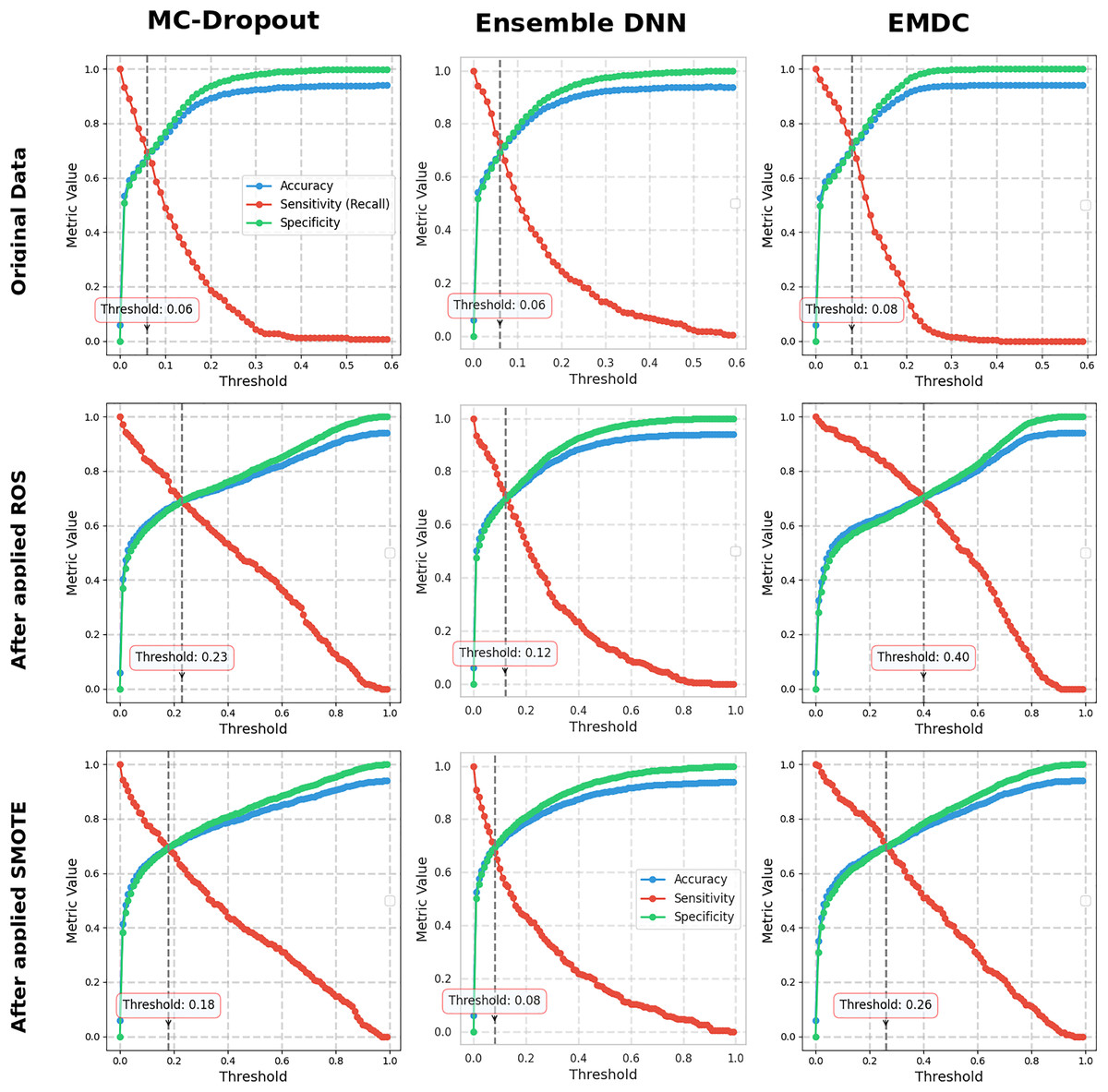
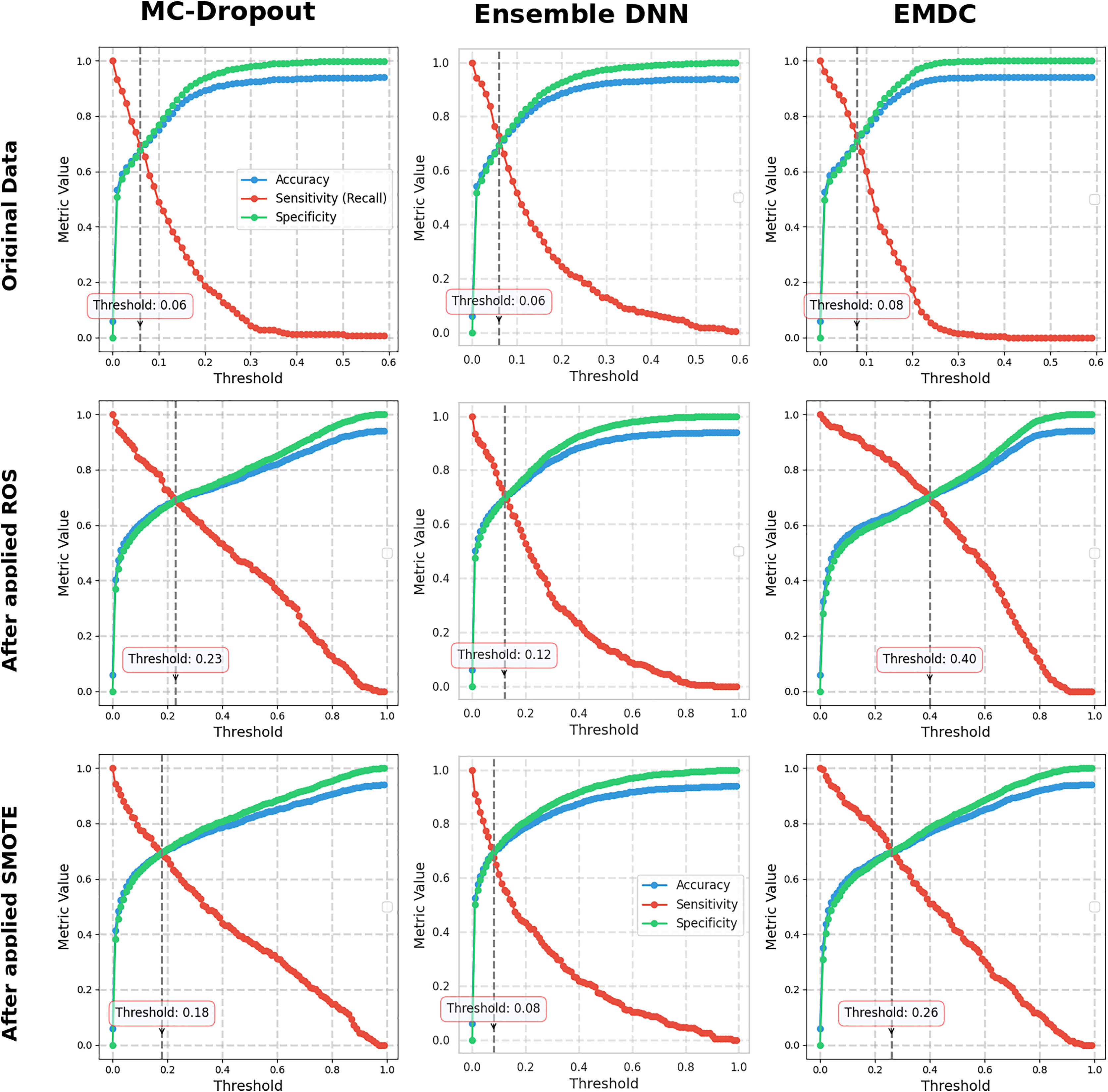
Figure 2: Performance metrics at different thresholds.

Download full-size image

DOI: 10.7717/peerj-cs.3365/fig-2

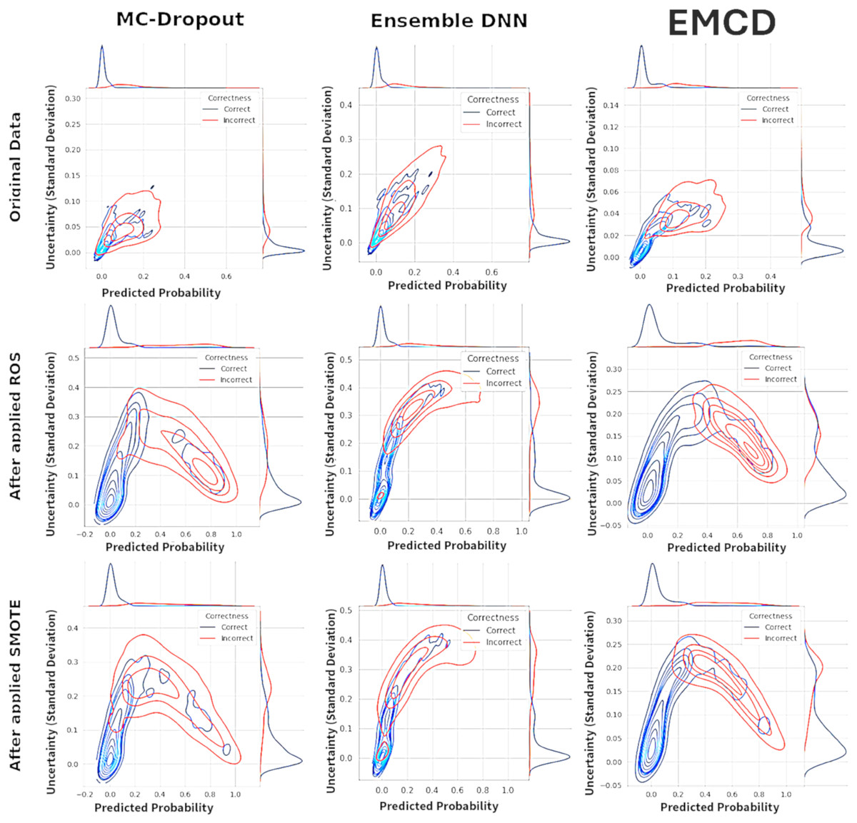
Figure 3: Kernel density estimation (KDE).

Download full-size image

DOI: 10.7717/peerj-cs.3365/fig-3

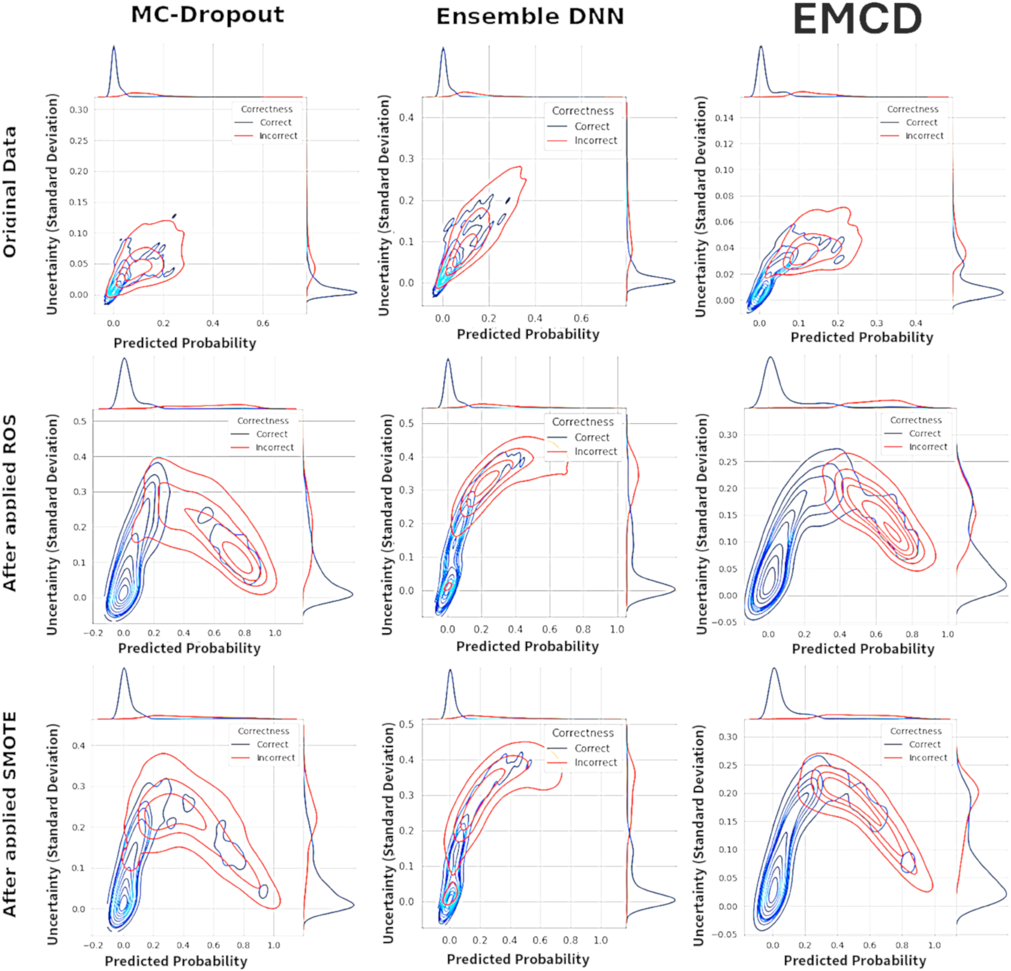
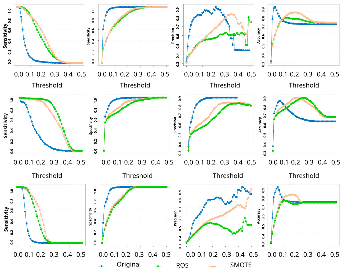
Figure 4: Uncertainty confusion matrix: predictive-uncertainty curves for sensitivity, specificity, precision, and accuracy vs decision threshold.
Rows indicate the uncertainty method, top: MCD; middle: Deep Ensemble; bottom: EMCD. Each panel compares the baseline model (no resampling) with SMOTE and ROS.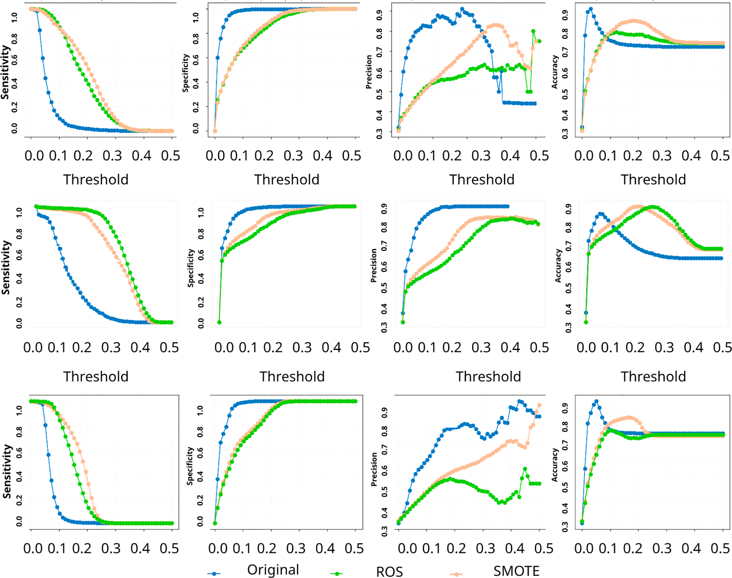

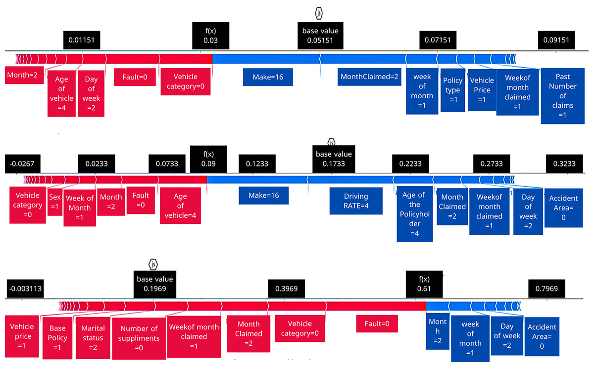
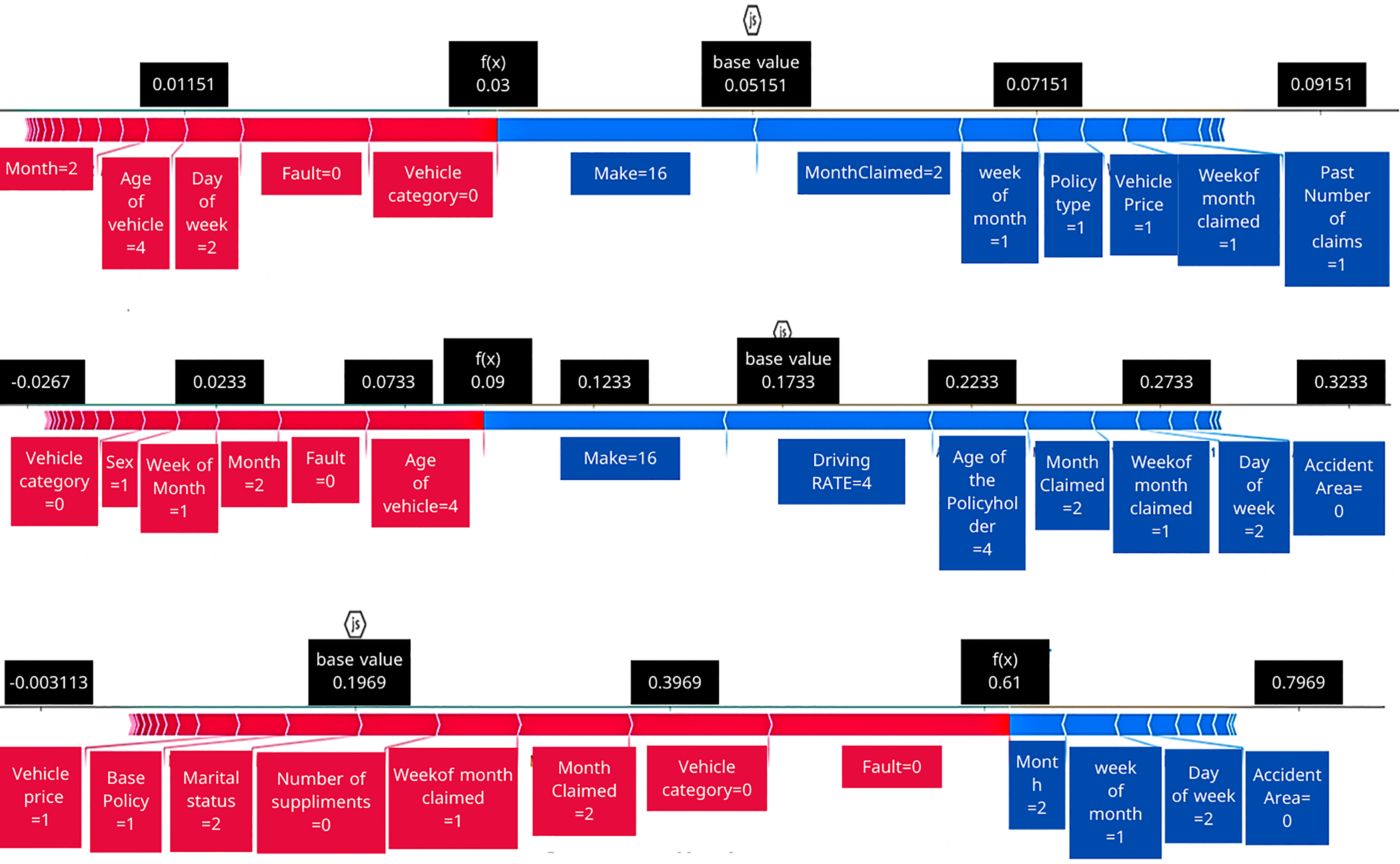
Download full-size image

DOI: 10.7717/peerj-cs.3365/fig-4

Figure 5: SHAP force plots comparing feature impact across original, ROS, and SMOTE-processed datasets.

Download full-size image

DOI: 10.7717/peerj-cs.3365/fig-5

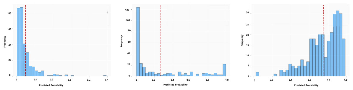
Figure 6: MC dropout predictions for one test instance.

Download full-size image

DOI: 10.7717/peerj-cs.3365/fig-6

Table 4 reports mean predicted fraud probabilities for each true class and the across-case standard deviation (SD) for three uncertainty-aware models under different rebalancing regimes. Two consistent effects appear after rebalancing (ROS/SMOTE): (i) a score lift, higher average fraud scores for both classes; and (ii) greater class separation in score space. The separation $Δ = \bar{p} (f r a u d | y = 1) - \bar{p} (f r a u d | y = 0)$ rises from ~0.08 to 0.10 on the original data to 0.28–0.34 after rebalancing (largest for EMCD + SMOTE: 0.344).

Original dataset. All methods are conservative. EMCD is the most concentrated (lowest SD: 0.069/0.094) with intermediate means (0.054/0.134), the ensemble is slightly more dispersed (0.093/0.129) and assigns the highest fraud mean (0.150), and MCD sits between them.
ROS. MCD shows the largest shift (fraud mean 0.476; SD 0.298 ≈ 3× its original), the ensemble moves more moderately (0.278; SD 0.213), and EMCD assigns the highest fraud mean (0.512) with increased dispersion (SD 0.242) though still below MCD’s SD.
SMOTE. Patterns mirror ROS quantitatively: MCD remains elevated (0.452; SD 0.287), the ensemble stays intermediate (0.288; SD 0.246), and EMCD is most assertive (0.538; SD 0.260), delivering the largest separation overall.

Implications. EMCD is the most sensitive to minority amplification (highest fraud means; largest $Δ$ with SMOTE), the ensemble is more conservative and stable, and MCD is most susceptible to rebalancing in both central tendency and dispersion.

In any classification task, the choice of decision threshold (the cut-off probability for classifying a case as fraud) significantly influences performance. In this study, we determined an optimal threshold by examining the balance among three metrics: overall accuracy, sensitivity (true positive rate), and specificity (true negative rate). Rather than defaulting to 0.5, we identified the threshold at which these metrics were most aligned—effectively the point where their values were as close to each other as possible, minimizing the variance between them. This approach yields a threshold that avoids maximizing one metric at the extreme expense of the others, thus ensuring a more balanced performance. It is worth noting that in real-world applications (especially in the insurance domain), this theoretically optimal threshold might be adjusted based on practical considerations. For instance, if fraud prevention is paramount, one might lower the threshold to catch more fraud at the cost of more false alarms; if false accusations are a big concern, one might raise the threshold. Ultimately, the chosen cut-off should reflect an acceptable trade-off for stakeholders.

Figure 2 illustrates how model performance varies with different classification probability thresholds for each uncertainty quantification method, across the original and resampled datasets. From these curves, a clear pattern emerges regarding the effect of data rebalancing on performance. Notably, applying ROS or SMOTE leads to a marked increase in sensitivity for all three UQ methods. In other words, after using these oversampling techniques, the models became much better at correctly identifying fraudulent cases (higher true positive rates) across the board. Encouragingly, this improvement in sensitivity comes with only a minor impact on specificity and accuracy over a broad range of thresholds. The figure shows that the accuracy and specificity curves remain relatively stable (or drop only slightly) when moving to resampled data, even as the sensitivity curve shifts upward. This suggests that oversampling successfully boosts the detection of fraud with a relatively small trade-off in terms of false positives. For our dataset, enriching the training set with more fraudulent examples (via ROS or SMOTE) pushed the classifier to be more fraud-sensitive (catch more fraud), without dramatically eroding its ability to recognize legitimate claims. This finding is practically significant: it implies that when the goal is to capture more fraudulent instances, resampling the training data can be an effective strategy to shift the model towards a more sensitive operating point, all while maintaining an acceptable level of overall accuracy.

Figure 3 presents kernel density estimation contour plots examining the relationship between predicted fraud probabilities and associated uncertainty estimates across three uncertainty quantification methods. The visualization compares the distribution patterns of correctly classified instances (blue contours) against misclassified instances (red contours) to assess whether uncertainty estimates provide meaningful discrimination between accurate and inaccurate predictions.

Under the original imbalanced data conditions, all three methods exhibit substantial overlap between correct and incorrect prediction distributions. The contour patterns show considerable similarity in both central tendencies and dispersions, indicating that uncertainty estimates provide limited discriminative information for identifying misclassified instances. This overlap suggests that the uncertainty measures fail to effectively distinguish between reliable and unreliable predictions, potentially limiting their practical utility for fraud detection applications.

Following the application of ROS and SMOTE rebalancing procedures, the uncertainty distributions demonstrate markedly improved separation characteristics. The correctly classified instances (blue contours) concentrate in regions of lower uncertainty, while misclassified instances (red contours) shift toward higher uncertainty regions. This enhanced separation is particularly pronounced for the EMCD method under SMOTE conditions, where the red and blue contour regions show minimal overlap.

The observed separation patterns suggest that rebalancing techniques enhance the discriminative capacity of uncertainty estimates for identifying potentially erroneous predictions. MCD shows moderate improvement in uncertainty discrimination following rebalancing, with clearer distinction between correct and incorrect prediction regions. The Ensemble method demonstrates similar patterns with somewhat more diffuse boundaries. EMCD exhibits the most pronounced separation, particularly under SMOTE preprocessing, indicating potentially superior uncertainty informativeness for practical deployment scenarios.

The enhanced separation between correct and incorrect predictions in uncertainty space following rebalancing represents a potentially valuable characteristic for operational fraud detection systems. Predictions associated with higher uncertainty estimates may warrant additional scrutiny or manual review, while lower uncertainty predictions may proceed through automated processing pipelines. However, these distributional improvements should be validated through formal calibration analysis to ensure that uncertainty estimates accurately reflect prediction reliability rather than merely providing ordinal ranking capabilities.

This analysis indicates that the choice of rebalancing technique significantly influences not only prediction accuracy but also the informativeness of associated uncertainty estimates, with implications for both model selection and operational deployment strategies.

To assess the practical utility of uncertainty estimates, we employed an uncertainty confusion matrix that evaluates whether models appropriately signal their prediction reliability. This framework treats uncertainty estimation as a binary classification task: for each prediction, we determine whether it should be classified as “certain” or “uncertain” based on a predetermined threshold.

Matrix construction and interpretation

The uncertainty confusion matrix (Fig. 1) cross-tabulates prediction correctness (True/False) with uncertainty classification (Certain/Uncertain), yielding four distinct categories:

True certainty (TC): Correct predictions with low uncertainty (ideal scenario)
True uncertainty (TU): Incorrect predictions with high uncertainty (desirable error flagging)
False uncertainty (FU): Correct predictions unnecessarily flagged as uncertain (conservative overestimation)
False certainty (FC): Incorrect predictions with low uncertainty (dangerous overconfidence)

The optimal scenario combines high TC and TU counts while minimizing FC cases, which represent confidently incorrect predictions, particularly problematic in fraud detection contexts.

Figure 4 demonstrates the sensitivity of these metrics to uncertainty threshold selection. Lower thresholds (0.1) maximize error detection (high USen) but generate more false uncertainty flags (lower UPre). Higher thresholds (0.5) reduce false alarms but risk missing genuine errors. This trade-off reflects a fundamental challenge in uncertainty-based fraud detection systems: balancing comprehensive error detection against operational efficiency. The analysis reveals that rebalancing techniques enhance uncertainty informativeness, models become better at distinguishing their reliable from unreliable predictions. However, the persistent moderate UPre values across all methods indicate that uncertainty flags, while valuable for error detection, require integration with domain expertise and operational workflows rather than serving as standalone decision criteria.

SHAP-based interpretability of predictions

In addition to quantitative performance, we analyzed individual predictions using SHAP to interpret how features contribute to the fraud prediction and how these contributions change with different training data balances. Figure 5 illustrates SHAP force plots for a single representative instance under three scenarios: using the original dataset, using ROS, and using SMOTE. In each subplot, the base value (the model’s average predicted fraud probability over the training set) is indicated as the starting point. Features pushing the prediction higher (toward fraud) are shown with arrows pointing to the right (typically colored red), and features pushing the prediction lower (toward non-fraud) are shown with arrows pointing to the left (colored blue). The length of each arrow reflects the magnitude of that feature’s contribution to the deviation from the base value. This visualization allows us to decompose the model’s output for the instance into positive and negative feature influences. Notably, although the underlying instance is the same, the pattern of feature contributions is not static: certain input variables have different impacts on the prediction across the three datasets. For example, a feature that strongly increased fraud probability in the original data model might have a more muted effect after SMOTE, or vice versa. These shifts imply that the resampling methods (ROS and SMOTE) altered the learned importance of features in the model. In other words, balancing the training data not only affected overall performance and uncertainty, but also changed the model’s internal reasoning for this prediction. This could be due to the model relying on different fraud indicators once minority class examples are more prevalent. The SHAP analysis thus provides transparency into how the model’s decision logic adapts when the training data distribution is modified.

To complement the force plots, Fig. 6 provides a view of the model’s predicted probability distribution for the same test instance under each scenario, highlighting the model’s confidence in its prediction. (In the case of MCD, for instance, this could be the distribution of predictions from multiple stochastic forward passes.) Figure 6 enables a direct comparison of both the prediction accuracy and confidence for that particular instance across the original, ROS, and SMOTE-trained models. A striking observation is the difference in prediction confidence for incorrect vs. correct predictions. In the original dataset scenario, the model’s prediction for this instance was incorrect the mean = 0.046 yet made with high confidence with low SD = 0.05477 (the model was overly sure in a wrong fraud/not-fraud decision). This is a problematic situation, as it reflects the model’s unwarranted assurance in a mistaken judgment, a critical issue for trust in an AI system. In contrast, with the ROS-trained model, the prediction for the same instance was still incorrect the mean 0.2729, but the model was appropriately uncertain about it, the distribution in Fig. 6 for ROS shows a high variance (large SD = 0.343), indicating low confidence. In essence, after ROS the model “knew that it didn’t know” the correct class for this case, which is a safer outcome than being confidently wrong. Finally, the SMOTE-trained model correctly predicted the instance’s class the mean = 0.748 and did so with a high confidence (the distribution is narrow, indicating low variance around a correct prediction with low SD = 0.1771). This outcome, a correct and confident prediction, is the ideal scenario and showcases the potential benefit of the SMOTE resampling method in this example. The comparison across these three cases highlights a few important points. First, data imbalance in the original set led the model to be overconfident in certain wrong predictions, which can be dangerous in practice. Second, ROS helped the model recognize its uncertainty in a difficult case (preventing overconfidence, even though it didn’t fully fix the error), thereby adding a layer of caution to the decision. Third, the more sophisticated SMOTE oversampling not only improved the accuracy for this instance but also maintained strong confidence when it was correct, illustrating that the model’s calibration can improve alongside accuracy. In summary, the SHAP-based interpretability analysis, in tandem with uncertainty measures, provides a deeper understanding of why the models made certain predictions and how sure they were about them. This dual perspective is crucial for moving “from prediction to trust”: it shows whether we can trust a prediction’s reliability and offers insights into the model’s decision factors, which is invaluable for stakeholders in insurance fraud detection.

Conclusion, future work, and limitation

In this research, we explored advanced deep learning models for automobile insurance fraud detection with a focus on UQ to enhance trust and transparency in predictions. We introduced a refined uncertainty confusion matrix along with multiple performance metrics to rigorously evaluate how well the models know what they don’t know. Our comparative study of three UQ techniques, MCD, deep ensembles, and an EMCD hybrid, revealed important insights into their effectiveness. While deep neural networks are powerful for fraud detection, they traditionally lack mechanisms to express confidence in their predictions. By applying MCD, ensemble, and EMCD methods, we addressed this limitation and showed that it is possible to obtain not just a fraud prediction but also a measure of confidence or uncertainty associated with that prediction.

Among the methods tested, ensemble-based approaches proved especially effective in capturing predictive uncertainty. In particular, the deep ensemble (aggregation of multiple DNNs) demonstrated robust performance, leveraging the diversity of its members to counteract individual model weaknesses. The EMCD method, which combines ensembling with MCD, further boosted the detection of fraudulent cases—consistently yielding the highest true positive rates in our experiments—but often at the cost of increased uncertainty. In contrast, the standard MCD approach (a single model with dropout-based sampling) improved the model’s ability to signal uncertainty yet was somewhat less aggressive in identifying fraud than EMCD. On balance, the deep ensemble without dropout emerged as a favorable approach due to its ability to reduce overfitting to any one set of weights and provide more stable predictions; it offered a good compromise between detecting fraud and maintaining confidence in those detections. Our findings also underscore the influence of data resampling on model behavior: introducing ROS and SMOTE rebalancing significantly amplified the models’ uncertainty in many cases. Notably, this heightened uncertainty was strongly correlated with misclassifications, which suggests an intuitive result—many of the cases that the model struggles with (often minority-class edge cases) were exactly those introduced or given more weight by oversampling. This result offers a double-edged insight: on one hand, resampling improves detection of minority-class (fraud) instances, but on the other hand, it makes the model less certain overall, correctly reflecting that those newly emphasized cases are inherently harder to classify. From an application standpoint, this is useful information: it means the model will warn us (via higher uncertainty) when it is making predictions on the harder, resampled cases, aligning with our goal of making the AI’s decision process more transparent and trustworthy.

To summarize our key contributions: we have demonstrated that deep learning models for fraud detection can be significantly enhanced by integrating uncertainty quantification techniques, leading to more informative predictions that either come with high confidence or are flagged with appropriate uncertainty. We showed that the EMCD approach can detect the most fraud cases (highest sensitivity), whereas a plain ensemble offers more conservative and stable predictions, and MCD lies in between—each approach has merits depending on the operational priorities (catch-all vs. caution). We also reinforced the value of using an uncertainty confusion matrix and related metrics to statistically evaluate how well the model’s uncertainty estimates align with actual correctness. Finally, by incorporating SHAP interpretability, we added an explanatory layer to the black-box DNN, allowing us to trust the model’s decisions not just because of numeric performance, but because we can see reasons for those decisions and verify that they make domain sense.

Building on this work, there are several clear avenues for future research. First, future studies should explore optimizing ensemble techniques for even better uncertainty management. This could involve increasing the diversity or number of ensemble members, or investigating stacking and boosting frameworks, with the goal of reducing predictive variance without sacrificing fraud detection capability. Systematic ablation studies examining the individual contributions of ensemble size, Monte Carlo iteration counts, and architectural choices would provide deeper insights into optimal UQ configuration for fraud detection applications. Such studies could isolate the specific components of driving performance improvements and guide more principled hyperparameter selection. Additionally, our results on resampling point to the need for a deeper investigation into the dynamics between data balancing and model uncertainty. It would be worthwhile to examine different resampling ratios or more sophisticated synthetic data generation methods to see if one can attain the sensitivity benefits of oversampling without proportionally increasing uncertainty. Another promising direction is the development of hybrid UQ models that combine the strengths of multiple approaches. For example, techniques that blend Bayesian neural network principles with ensembles, or incorporate evidential deep learning, could potentially yield models that are both highly accurate and well-calibrated in their confidence. Such hybrids might address some limitations we observed (like the trade-off between uncertainty sensitivity and precision) by providing more nuanced uncertainty estimates. Moreover, extending the uncertainty quantification framework to multi-class or more complex fraud scenarios (beyond binary classification) and evaluating the methods on different types of insurance fraud (e.g., health or life insurance fraud) would test the generality and robustness of our conclusions. We also suggest future work on integrating these models into a human-in-the-loop system: since our findings indicate that high-uncertainty predictions are a useful signal, a practical system could automatically queue up those cases for manual review. Research into how human experts interpret the model’s explanations and uncertainty, and how their feedback could be used to further retrain or fine-tune the model, would be invaluable for deploying AI fraud detectors in the field.

In conclusion, this study advances the field of insurance fraud detection by not only improving prediction accuracy through modern deep learning techniques but also by transforming the predictive process into one that is more transparent and trustworthy. By quantifying and analyzing uncertainty, and by explaining individual predictions, we move a step closer to AI systems that industry professionals can rely on with greater confidence. The comparative performance analysis of MCD, ensemble, and EMCD approaches provides guidance on model selection depending on an organization’s priorities, and the highlighted future directions aim to further enhance the reliability, interpretability, and overall effectiveness of fraud detection models in insurance and beyond.

Our study has several key limitations: first, we evaluated our UQ techniques on a single-year auto-insurance fraud dataset from Oracle, so our findings may not apply to other insurance lines (e.g., life), jurisdictions with different fraud patterns, or datasets featuring alternative variables and fraud prevalences; second, our framework focuses solely on binary classification whereas real-world fraud detection often requires multi-class or multi-label modeling that could exhibit very different uncertainty behaviors; and third, we compared only three UQ methods (MCD, deep ensembles, and EMCD), omitting emerging approaches such as Bayesian neural networks, evidential deep learning, and hybrid stacking or boosting ensembles that might offer improved calibration or computational efficiency.

Supplemental Information