
Transfer learning approaches for EfficientNetV2 B0 and ImageNet skin cancer classification in a convolutional neural network
- Published
- Accepted
- Received
- Academic Editor
- Consolato Sergi
- Subject Areas
- Computer Vision, Data Mining and Machine Learning, Neural Networks
- Keywords
- Skin cancer detection, Skin lesion, Deep learning algorithms, Convolutional neural networks, Image augmentation, EfficientNetV2 B0, ImageNet
- Copyright
- © 2025 Karthiha and Allwin
- Licence
- This is an open access article distributed under the terms of the Creative Commons Attribution License, which permits unrestricted use, distribution, reproduction and adaptation in any medium and for any purpose provided that it is properly attributed. For attribution, the original author(s), title, publication source (PeerJ Computer Science) and either DOI or URL of the article must be cited.
- Cite this article
- 2025. Transfer learning approaches for EfficientNetV2 B0 and ImageNet skin cancer classification in a convolutional neural network. PeerJ Computer Science 11:e3362 https://doi.org/10.7717/peerj-cs.3362
Abstract
Early skin cancer detection by visual inspection of skin lesion images may be challenging. In recent years, there have been impressive findings from research into the use of deep learning algorithms to assist in identifying skin cancer. Modern techniques are more sensitive, specific, and accurate than dermatologists. However, dermoscopy image analysis using deep learning models still faces some challenges. Image segmentation, noise filtering, and inconsistent capture settings are all examples of such tasks. Melanoma, the deadliest form of skin cancer, is on the rise in occurrence. Early detection is crucial for preventing the spread of skin cancer. An automated technology that can detect skin cancer independently of human doctors is introduced in this study. Everyone offers a transfer learning-based approach to melanoma lesion detection. The images taken with the proposed technology are first preprocessed to remove noise and lighting influences. An important part of deep learning is image augmentation. Here are a few ways to make your images seem better. Image augmentation, which involves enlarging the training images, may improve the learning phase’s effectiveness. An innovative deep transfer learning technique for melanoma classification is proposed in this article using EfficientNet V2 B0 and ImageNet. To identify malignant skin lesions in a sample, two deep convolutional neural networks may be used: MobileNetV2 and ImageNet. We test the proposed deep learning model on the ISIC 2020 dataset. The suspicious spot in the middle of the image becomes the focus point at each stage. The combined results from these parts are put into a fully connected neural network. Results from experiments demonstrate that the proposed technique outperforms state-of-the-art deep learning algorithms in terms of accuracy while using fewer computational resources.
Introduction
The unchecked growth of aberrant skin cells is the root cause of skin cancer, a malignant tumor. In most cases, these malignancies are caused by prolonged exposure to ultraviolet (UV) rays on unprotected skin (Factors, 2019; Gandhi & Kampp, 2015; Snyder et al., 2020). Of all skin malignancies, 99% are basal cell carcinomas or squamous cell carcinomas, whereas only 1% are melanomas (American Academy of Dermatology, 2025). It is one of the most common and potentially fatal diseases in the US. There are more than five million cases of different skin disorders reported each year in the United States (Rogers et al., 2015). The incidence of skin cancer has been rising during the past few years (Whiteman, Green & Olsen, 2016). Melanoma is the deadliest kind of skin cancer, accounting for around 75% of all skin cancer-related fatalities (Xie et al., 2017). The National Cancer Institute predicts that there will be about 99,780 additional instances of melanoma in 2022, involving 57,100 males and 42,600 women affected. There are around 7,650 people whose lives are cut short by melanoma. Specifically, melanoma affects the squamous cell layer’s melanocytes. Depending on how bad the cancer cells are, there could be more subcategories of benign and malignant. A benign growth on the skin does not have any cancerous cells. Early treatment is necessary due to the high concentration of cancerous cells in benign tumors (Dalila et al., 2017). New data show that the survival rate for melanoma patients is 99% if the disease is detected before it extends to the lymph nodes.
Dermatologists have lately started diagnosing skin cancer using dermoscopy, which is a clinical technique (Vestergaard et al., 2008). Additionally utilized is data on the person’s social habits, ethnicity, history of skin diseases, sun exposure, and other personal information is utilized. However, when it comes to diagnosing specific skin cancers, this approach is often linked to a significant risk of error for less skilled medical professionals and inconsistent outcomes among dermatologists (Menzies et al., 2005). Computer-assisted methods for diagnosing skin cancer have advanced significantly in the last several decades, allowing for the clinical diagnosis of lethal types of skin cancer such as melanoma (Adegun & Viriri, 2018).
The GoogleNet Inception v3, a pre-trained convolutional neural network (CNN) model, has shown superior performance compared to dermatologists. Subsequently, researchers have used diverse deep learning (DL) methods and have enhanced their precision across a spectrum of dermoscopy databases (Albahar, 2019; Demir, Yilmaz & Kose, 2019; Hosny, Kassem & Foaud, 2019). Although the results seem promising, there are still notable concerns with the techniques, such as variations in skin physical appearance, including variances in lesion size, shape, and color; interference from objects in the image; and variable lighting and illumination settings during image collection. Irregular and fuzzy skin lesion margins may sometimes confuse detector algorithms (Al-masni et al., 2018; Naji, Jalab & Kareem, 2019).
Clinical images, dermoscopy images, and histopathology images are the three main types of images used by scientists to detect and classify skin malignancies. Because of their accessibility and prevalence in dermatological practice, dermoscopic images are the focus of this investigation. Furthermore, researchers in this area have access to a large amount of publicly accessible data. Table 1 shows that dermoscopy datasets that are accessible to the public are mostly sourced from the International Skin Imaging Collaboration (ISIC). Here is a list of the databases: References: (Goyal et al., 2020; Wen et al., 2022).
| Dataset name | Quantity of images | Dataset company |
|---|---|---|
| ISIC2016 | 900 | ISIC |
| ISIC2017 | 1,300 | ISIC |
| ISIC2018 | 12,000 | ISIC |
| ISIC2019 | 25,000 | ISIC |
| ISIC2020 | 43,000 | ISIC |
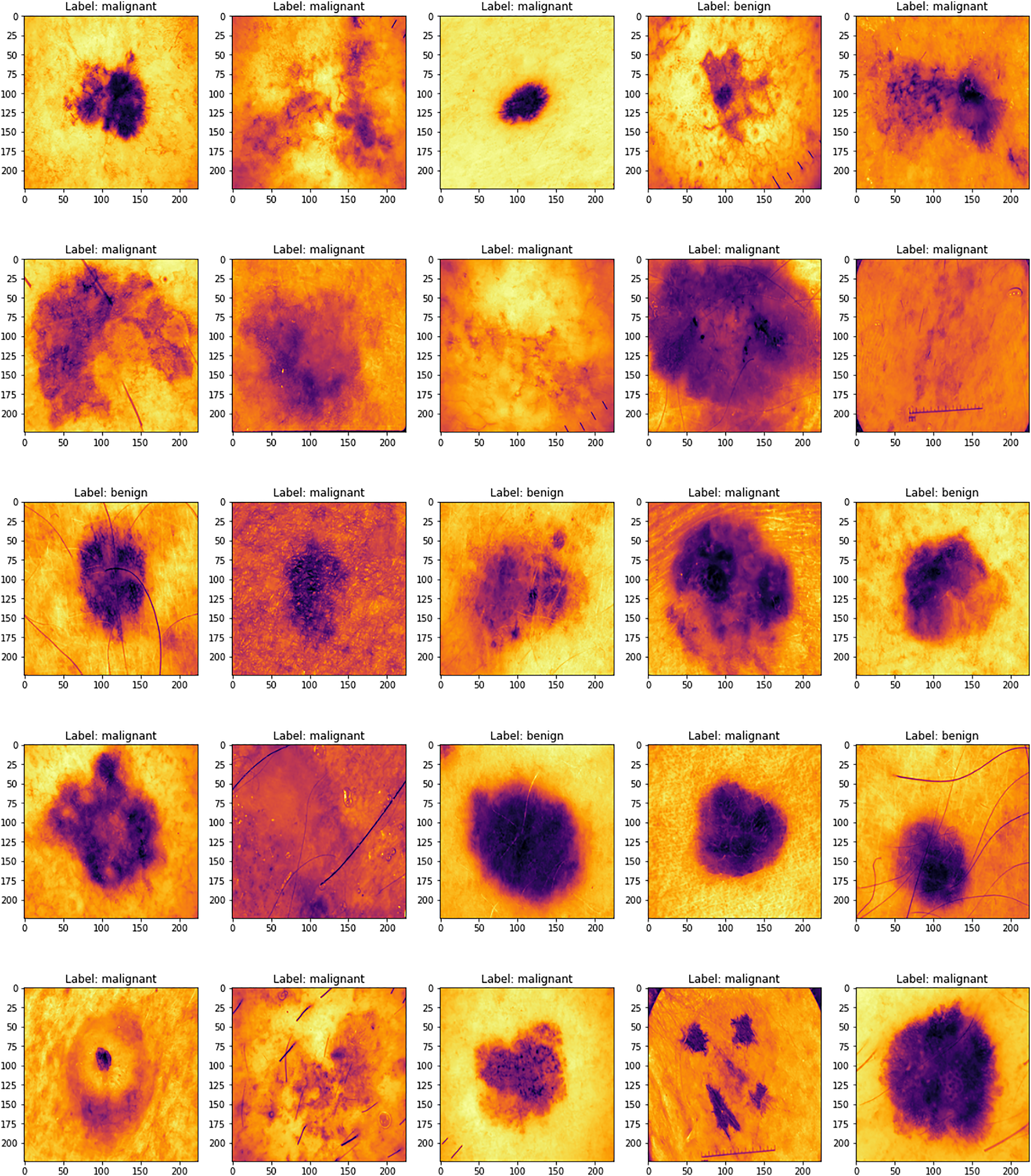
Figure 1 displays several sample images taken from the 2019 dataset of the International Skin Imaging Collaboration, which includes eight different types of skin cancers. Using a high-resolution lens and the right illumination, dermoscopy may be used to examine skin problems. Research using dermoscopy images has recently grown in prominence as a primary data set for artificial intelligence (AI) studies. The quantity of images in public databases has allowed researchers to create astonishing findings.
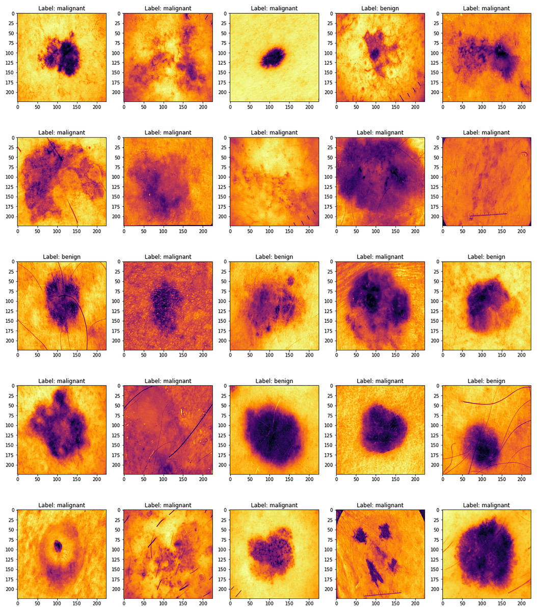
Figure 1: ISIC dataset samples.
Skin cancer is a major topic of our research since it is a global health problem. To better detect and diagnose skin cancers, especially fatal melanoma, there is a fantastic opportunity to use recent advances in deep learning and machine learning. There has been progress, but there are still big obstacles to overcome before computational techniques can accurately diagnose skin cancer. These include the fact that lesions don’t always look the same and the limitations of the diagnostic tools that are available. The current status of machine learning methods for skin cancer diagnosis is going to be the focus of this investigation. Both traditional approaches and cutting-edge deep learning methods are examined.
The methods and results of recent investigations are reviewed and evaluated in this work. Not only does it detail the work that has been done, but it also finds the gaps that still need to be filled for future studies. To encourage early intervention and obtain better treatment outcomes, it is vital to increase the accuracy, reliability, and accessibility of skin cancer diagnostics.
Additionally, unlike other evaluations, this one classifies different machine learning algorithms in great detail. We expand the prior research on deep learning approaches to skin cancer classification by analyzing subsets such as supervised, semi-supervised, reinforcement learning, and ensemble techniques (Wu et al., 2022; Dildar et al., 2021). Our analysis covers a wider variety of models, including transformers, in contrast to the study (Bhatt et al., 2023), which just dealt with CNNs within the deep learning spectrum.
Background
Unsurprisingly, skin cancer is the most prevalent kind of cancer in humans, since the skin is the largest organ in the body (Ashraf et al., 2020). There are two primary classifications of skin cancers: melanoma and non-melanoma (Byrd, Belkaid & Segre, 2018). Prompt identification is essential for this malignant condition, as it is for other malignant conditions. Melanoma is the most lethal kind of skin cancer (Elgamal, 2013). It happens when the proliferation of melanocyte cells becomes uncontrolled. Although it may occur in any location, the probability of it occurring in places exposed to the sun is greater. Now, the only means of identifying skin cancer is by a biopsy, which involves extracting a sample from the skin to determine whether it is malignant (American Cancer Society, 2021). Utilizing an automated detection technology to assist clinicians in promptly diagnosing cancer is advisable, given the occurrence of medical mistakes. Utilizing machine learning methods enables a much more expedited cancer diagnosis approach. Deep learning has emerged as one of the most successful methods for detecting and identifying objects in the last ten years (Dildar et al., 2021).
Feature extraction and classification are carried out in tandem in a single step in deep learning architectures. When working with images, it is essential to get the traits from locations that are more likely to have the needed data. The bulk of the skin patches that need attention are located in the middle part of the image in datasets relevant to skin cancer (see Fig. 1). This information has been used to improve the feature extraction procedure in this study. After training three separate CNNs, their outputs are combined and inputted into a single fully connected neural network (FCN). Using this specific combination improved the detection rate, according to the data.
Novelty justification
This study uses CNNs to classify skin cancer with great accuracy by combining EfficientNetV2 with ImageNet-based transfer learning. In contrast to previous research, the suggested study tackles class imbalance concerns that were often overlooked in earlier models and places a strong emphasis on cross-validation and external dataset testing. To provide more clinical relevance, the model also focuses on enhancing generalization across various skin types and lesion variants. Additionally, this study offers a clearer and reliable diagnostic approach by integrating interpretability methods, including confusion matrix assessment and Receiver Operating Characteristic (ROC) analysis. All of these factors work together to advance trustworthy and practical AI-driven dermatological diagnoses.
Motivation
If not detected early, skin cancer may be fatal; deep learning can improve early detection using EfficientNetV2 and ImageNet.
By lowering the need for large labeled datasets, transfer learning improves the viability and precision of skin cancer classification.
EfficientNetV2 optimizes CNN-based medical image analysis by offering increased accuracy and processing economy.
Transfer learning improves generalization by enabling efficient model training even with small medical image datasets.
Medical practitioners may diagnose skin cancer more quickly, accurately, and easily when deep learning is used in dermatology.
Contribution
Utilized pre-trained EfficientNetV2 B0 and ImageNet models to provide precise skin cancer classification with less labeled dermatological data, hence decreasing training duration and enhancing convergence.
Employed the advanced feature extraction capabilities of CNNs, particularly EfficientNetV2 B0, to discern intricate patterns in dermoscopic images, hence enhancing classification accuracy between benign and malignant categories.
Proven that transfer learning substantially improves model generalization, attaining elevated accuracy and resilience, hence rendering it appropriate for practical medical diagnostic applications in contexts with limited annotated data.
There are four main parts to this study. The literature review, methodology, and application of DL and Transfer Learning (TL) are all described in depth in the “Methods” section. The “Results” section details the outcomes and how they stack up against competing methods. A synopsis of the results and suggestions for further study are given in the “Discussion” section.
Related works
Several studies have focused on the topic of skin cancer. We shall expeditiously review the several methodologies that have been used so far. Ali & Al-Marzouqi (2017) achieved classification using LightNet. Their approach was well-suited for mobile applications. The metrics utilized to report the results after testing the 2016 datasets from the International Skin Imaging Collaboration (ISIC) were accuracy (81.60%), sensitivity (14.90%), and specificity (98.00%) (Ali & Al-Marzouqi, 2017). Dorj et al. (2018) used a mixture of deep support vector machines (SVMs) to detect many types of skin cancers, such as melanoma, basal cell carcinoma (BCC), and squamous cell carcinoma (SCC). Non-melanoma malignancies, such as basal cell carcinoma and squamous cell carcinoma, cannot spread to other parts of the body and are more readily detectable compared to melanoma tumors (Dorj et al., 2018). The algorithm was tested on a total of 3,753 images, out of which four showed instances of skin cancer. Their highest level of accuracy was 95.1% for SCC, the ability to correctly identify actinic keratosis was 98.9%, and the ability to correctly identify SCC was 94.17%. The respective minimal values were 90.74% for melanoma, 96.9% for SCC, and 91.8% for BCC (Esteva et al., 2017). Esteva et al. (2017) used CNN to categorize the images into three unique categories. Melanoma, benign seborrheic keratosis (SK), and benign keratinocyte carcinomas (Codella et al., 2015) are the conditions being referred to. The detection of skin cancer was achieved by the use of a hybrid system that included support vector machines (SVMs), sparse coding, and deep learning techniques (Harangi, Baran & Hajdu, 2018). The clinical records consisted of 2,624 cases of melanoma, 144 cases of atypical nevi, and 2,146 cases of benign lesions, all of which were included in the ISIC dataset. The evaluation included twenty rounds of two-fold cross-validation. Two classification tasks were presented: (I) distinguishing melanoma from all non-melanoma lesions, and (II) distinguishing melanoma from atypical lesions alone. The first test yielded a recall rate of 94.9%, a specificity rate of 92.8%, and an accuracy rate of 73.9%. In contrast, the subsequent task resulted in a recall rate of 73.8%, a specificity rate of 74.3%, and an accuracy rate of 93.1%.
Harangi, Baran & Hajdu (2018) used CNNs that integrated the architectures of AlexNet, Visual Geometry Group Network (VGGNet), and GoogleNet (Srividhya et al., 2019). Kaloucheuse used a CNN that was trained specifically on edge detection to accurately identify instances of skin cancer (Rezvantalab, Safigholi & Karimijeshni, 2018). A study done by Rezvantalab, Safigholi & Karimijeshni (2018) showed that deep learning models, namely DenseNet201, Inception v3, ResNet 152, and InceptionResNet v2, had superior performance compared to other models, with a minimum improvement of 11%. Sagar & Jacob (2020) used ResNet-50 with deep transfer learning on a collection of 3,600 lesion images obtained from the ISIC dataset. When compared to InceptionV3, DenseNet169, and the recommended model, it exhibited superior performance (Sagar & Jacob, 2020). Acosta et al. (2021) used ResNet152 for classification after the extraction of the region of interest using a mask and a region-based CNN. In all, 2,742 images were selected from ISIC. Generative adversarial networks (GANs) and Progressive Generative Adversarial Networks (PGANs) served as the foundation for many subsequent publications. Rashid, Tanveer & Khan (2019) used GAN on the ISIC 2018 dataset. The disorders they sought to detect included malignant keratosis, vascular lesions, melanoma, dermatofibroma, and benign nevi. By using a deconvolutional network, they were able to get an accuracy rate of 86.1% (Rashid, Tanveer & Khan, 2019). Bisla et al. (2019) used a deep convolutional GAN and a decoupled deep convolutional GAN for their data augmentation. The datasets used were ISIC 2017 and ISIC 2018. Their accuracy percentage was 86.1% (Bisla et al., 2019). Ali & Al-Marzouqi (2017) used a self-attention-based PGAN to detect vascular, pigmented benign keratosis, pigmented Bowen’s, nevus, dermatofibroma, and other skin diseases. We used the ISIC 2018 dataset. An enhanced generative model was optimized by using a stabilizing technique. The accuracy was 70.1% with 19 instances correctly classified (Abdelhalim, Mohamed & Mahdy, 2021). Zunair & Hamza (2020) developed a two-stage framework for the automatic classification of skin lesion images. The study cited used adversarial training and transfer learning techniques (Zunair & Hamza, 2020). Some other references are listed in Table 2.
| Ref. | Dataset | Methods | Accuracy | Disease |
|---|---|---|---|---|
| Yu et al. (2019) | ISBI 2016 | DCNN-FV | 86.54% | Non-Melanoma challenge |
| Rokhana, Herulambang & Indraswari (2020) | ISIC Repository | DCNN | 84.76% | Benign, Malignant, Melanoma |
| Hu et al. (2019) | Ph2 | FSM & SVM | 91.90% | Malignant, Benign |
| Dalila et al. (2017) | Self-Contained 172 images | ANN | 93.6% | Malignant, Benign |
| Brinker et al. (2019) | Self-Contained 172 images | ResNet-50 | 82.3% | Melanoma |
| Mukherjee, Adhikari & Roy (2019) | Dermofit | CNN based CMLD model | 90.58% | Melanoma |
Clinical relevance
EfficientNetV2–based pipeline is intended as a triage and decision-support tool rather than a stand-alone diagnostician. In everyday dermatology practice, clinicians confront large backlogs of dermatoscopic images; the proposed model can automatically flag lesions with high malignancy probability, allowing dermatologists to (i) prioritize high-risk cases, (ii) reduce time to biopsy scheduling, and (iii) extend expert care to under-resourced or remote settings via tele dermatology. Because the model operates on standard dermatoscopic JPGs without hardware modifications, integration fits seamlessly into existing clinical workflows and electronic health record systems.
Limitation
A higher false negative rate results in missed early melanomas.
The model may output a benign probability is delayed treatment.
An active learning pipeline that flags low-confidence samples for expert labeling.
Methods and techniques
To classify melanoma skin cancer, this research introduces a complex transfer learning system. In the first step, we deal with the issue of class imbalance and introduce variability in the dataset by using pre-processing techniques and various augmentation approaches. To differentiate between benign and malignant melanoma skin lesions, the system employs a pre-trained EfficientNet V2 B0 and an ImageNet model at the second level after extracting automated features. The experiments are developed by Anaconda Python Jupyter notebook using Python language, Windows 10 OS, Intel i3, 8GB RAM, Tensorflow, Keras, Plotly, matplotlib, opencv python, pandas, and NumPy packages are installed in the project development requirements. The proposed method’s flowchart is shown in Fig. 2.
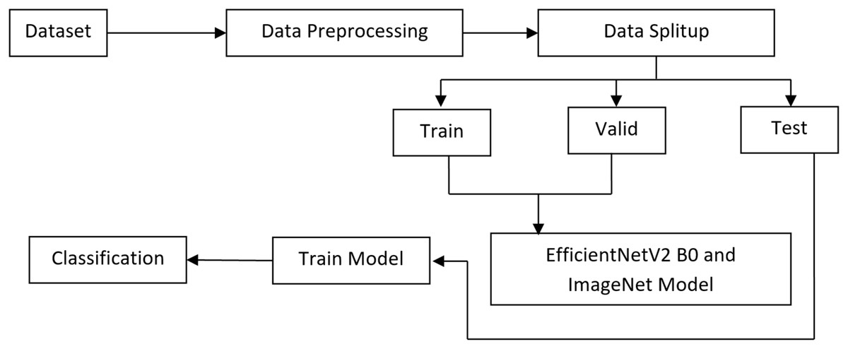
Figure 2: Proposed architecture.
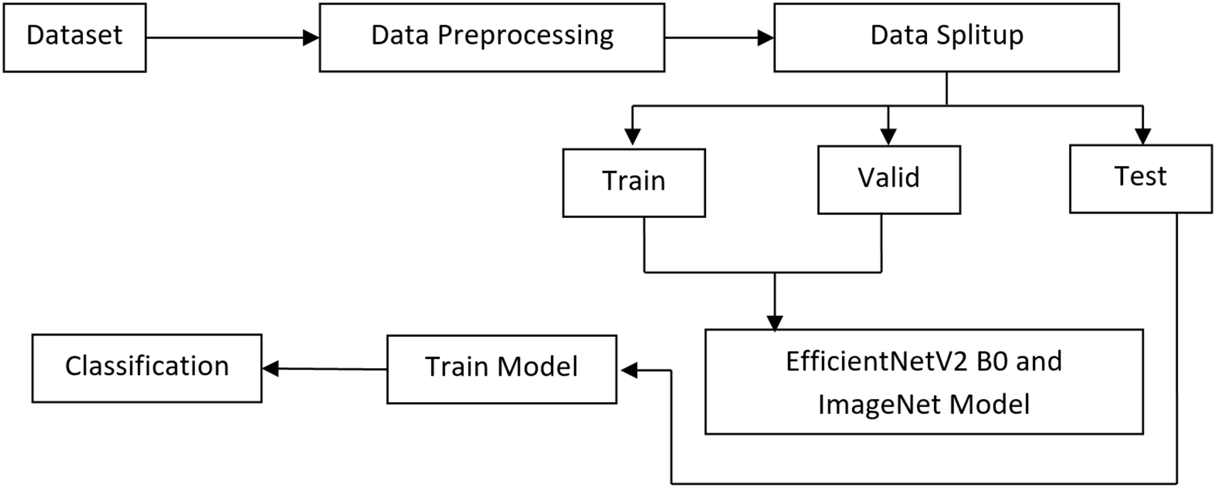
Dataset
Deep learning algorithms are reliant on the availability of a real and adequate dataset. Without such a dataset, these algorithms would not function well. The ISIC-2020 Archive has the most extensive collection of publicly available dermoscopy images of skin lesions. Various institutions submitted patient information from a diverse spectrum of ages and orientations. The collection comprises 33,126 dermoscopy images, with 584 depicting malignant skin lesions and 31,485 depicting benign skin lesions, collected from over 1995 people. By using unique patient IDs, every image is associated with a specific patient. There was a total of 620 shots of melanoma and 12,010 images of the benign class. The data from these two groups is imbalanced. To tackle the issue of class imbalance, ISIC 2020 has scored a total of 4,600 melanoma images in its collection. Subsequently, other data augmentation methods were used, including rescaling, width shift, rotation, shear range, horizontal flip, and channel shift, resulting in a total of 12,010 instances. To tackle the issue of class imbalance, we used a dataset of 12,010 harmless images. A random selection was made from the whole collection of images, namely from the ones belonging to the benign class. The dataset is available at https://challenge2020.isic-archive.com/. Figure 3 display many instances of the images.
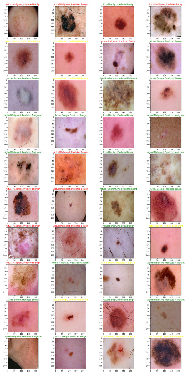
Figure 3: Benign and maligant.
ISIC Dataset Image.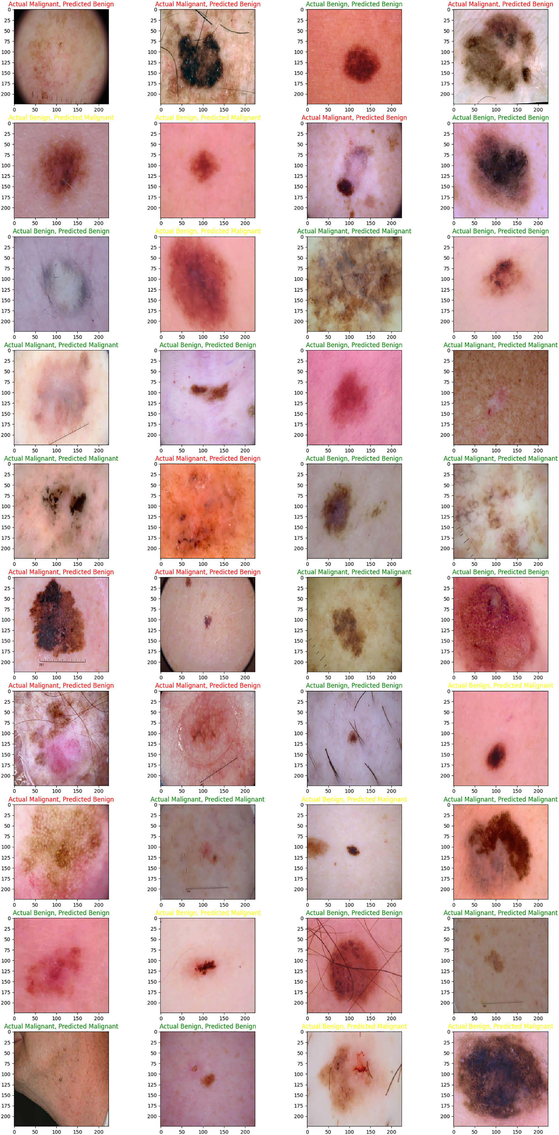
Data processing
All input images of the ISIC-2020 dataset undergo preprocessing to improve the features and produce more consistent classification results. To reduce the possibility of over-fitting, the CNN method calls for a large-scale image collection followed by frequent and thorough training. Preprocessing is a must when dealing with medical images. When doing preprocessing, keep in mind that there are two distinct tasks. Preprocessing the images is one way to address color problems and increase image quality. Part two focuses on data augmentation, which entails various means of supplementing the dataset with additional images. First, we standardized the images. The collection of images was made more consistent by removing the average RGB value. A massive quantity of images is needed for training and testing purposes to construct a robust CNN. In the battle against skin cancer, this is a huge hurdle. It takes a lot of time and effort to build huge databases that encompass many different kinds of cancer. The study makes use of the ISIC 2020 dataset.
Dermoscopy training images totalling 15,700 have been collected from 1995 individuals. A total of 3,050 images, or about 4% of the total, were selected for testing and kept apart from the others. Applying augmentation to the training set is the only way to make the model more robust and increase the number of examples it can generate. On the other hand, because it evaluates performance using actual images, the test set does not need augmentation. To improve the training dataset, the images were rotated by 10 degrees to generate 35 × 15,700 additional images.
Image resize
The preliminary ISIC dataset contains images with a size of 6,000 × 4,000. The dataset is rescaled to dimensions of 256 × 256. It will significantly decrease the model’s performance and accelerate the processing.
Data augmentation
The training set has been significantly improved using the image data creation tool from the Python Keras library. We aimed to counteract overfitting by increasing the dataset’s variety. A drop in computing cost was achieved by applying scale transformation and utilizing lower values for pixels within the same range. There was a strict range of 0–1 for the pixel value due to the 1/255 parameter value. We rotated the images by 25 degrees using the rotation transformation so that they would reach a specified angle. You may use the range transformation to horizontally change the images either way, with the dimension shift option set to 0.1. Training images were vertically shifted with a range parameter value of 0.1 for height shift. In shear transformation, one of the image axes remains unchanged while the other is stretched at an angle, the shear angle, to produce the desired effect. For this case, we settled on a shear ratio of 0.2. With the zoom range choice, the unplanned zoom transformation was carried out. With values more than 1.0, this metric describes an enlarged image, whereas with values less than 1.0, it describes a reduced image.
The outcome was a 0.2x magnification achieved through a zoom range. Flip was used to horizontally reflect the image. A range of 0.0 to 1.0 was used to regulate the brightness, with 0.0 representing the lowest and 1.0 the maximum. This led to the usage of a zoom range of 0.5 to 1.0. The channel shift transformations involve randomly shifting the channel values using a value from a specified range. With a channel shift range of 0.05 and fill mode set to the closest, this example was created. Table 3 shows the data.
| Transformations | Setting |
|---|---|
| Scale transformations | Range from 0 to 1 |
| Zoom transformations | 0.2 |
| Rotation transformations | 25° |
Dataset split-up
The ISIC-2020 dataset had three distinct sections: testing, validation, and training. The training set was used to train the EfficientNet V2 B0 model, whilst the test and validation datasets were employed to evaluate its performance. Consequently, we divided the dataset into three parts: 15% for validation, 15% for testing, and 70% for training.
The ISIC 2020 dataset for skin lesion classification challenge contains 33,126 dermoscopic images. These images come with corresponding metadata (patient, age, sex, lesion location) and are used for binary classification of melanoma vs. non-melanoma. Table 4 shows the class distribution for the ISIC-2020 dataset with 33,126 images.
| Class | Number of images | Percentage (%) |
|---|---|---|
| Melanoma | 584 | 1.76% |
| Non-Melanoma | 32,542 | 98.24% |
| Total | 33,126 | 100% |
The ISIC-2020 class distribution Table 5 shows, after splitting the 33,126 images into 70% training, 15% validation, and 15% testing, while maintaining class balance through stratified sampling.
| Class | Total images | Training (70%) | Validation (15%) | Testing (15%) |
|---|---|---|---|---|
| Melanoma | 584 | 409 | 88 | 87 |
| Non-Melanoma | 32,542 | 22,779 | 4,881 | 4,882 |
| Total | 33,126 | 23,188 | 4,969 | 4,969 (Gandhi & Kampp, 2015) |
Selection method
Max-pooling is a technique in CNNs where a fixed-size window slides over the feature map, and only the maximum value within the window is retained. This operation reduces the spatial dimension of the feature map, focusing on the most significant features.
In skin cancer detection, the important patterns are often local features that describe the lesion’s shape, texture, and color. Max-pooling helps reduce the amount of data while retaining these important local features, making the model more efficient and reducing overfitting. Max-pooling layers would be applied after each convolutional layer to reduce dimensionality and emphasize important patterns in regions of the skin lesion, which are critical for distinguishing between benign and malignant lesions.
Transfer learning models
Training a CNN is a challenging endeavour due to the need for a large number of images for both training and testing purposes. Transfer learning is used to address the issue of limited image availability, as well as to increase image quality. In transfer learning, a network utilizes the parameters of a neural network that has already been trained that was trained on a comparable image dataset, which we want to leverage. The dataset should include a sufficient number of samples. In this study, transfer learning was used in the following manner: initially, the network used the CNN weights for ImageNet and EfficientNet V2 B0 as its starting weights. It signifies that a CNN was completely trained using the ImageNet dataset. The final layer of this network, which is typically used for classifying 1,000 different classes in ImageNet, has been replaced with a softmax layer that is designed for binary classification. This new layer is used to distinguish between melanoma and non-melanoma classes. It is worth noting that instead of using the softmax function, the sigmoid function can also be employed for this purpose. The softmax layer consists of nodes that correspond to the total number of outcomes, and each node represents the likelihood of a certain output. During the subsequent phase, the backpropagation technique is used to modify the weights of the network in response to the mistake in the output. This process aims to optimize the weights, making the network more suited to accommodate the new classes. It is crucial to prevent significant changes in the weights; hence, a modest learning rate should be used. The learning rate is the hyperparameter used in neural networks to regulate the adjustment of the model in response to mistakes. Utilizing a high learning rate will result in complete degradation of the weights. Considering the application of back-propagation to a certain point might be regarded as a hyperparameter in the training process.
The study has not yet conducted a comprehensive analysis of the computational trade-offs associated with training distinct CNNs at different input sizes. Although this multi-scale design enhances feature learning and classification performance, it increases the computational cost due to memory use, training time, and energy consumption. This overhead might impede real-time deployment or use in situations with limited resources. A shared-weight method or an improved design that cuts down on redundancy without slowing down may be the subject of future studies.
The method used in this research is theoretically similar to the one in the other, but it is better organized and makes use of transfer learning to improve its efficiency. Three independent networks were trained using images and transfer learning techniques that were distinct from one another. First, to get images with their accurate dimensions, the dataset including malignant tissues should be processed using the aforementioned method. The tumor or malignant region is often located in the center of the image when skin cancer diagnostics are being conducted. The surrounding area is typically composed of healthy skin. The abundance of healthy skin tissue could confuse or trick the network during detection. This issue may be resolved in two ways.
There are two choices: segmentation or the suggested method. Using segmentation, medical imaging may be quickly and accurately divided into two parts: the malignant area and the healthy surrounding tissue. However, segmentation has limitations and has its own set of problems. There are flaws in the segmentation issue that impact the learning process, which is the biggest downside. Two further networks were trained using the suggested strategy. The first stage is halving the original image’s size before resizing it. In the third step, we resize and crop the original image by 75%. Figure 4 displays the images at 100%, 75%, and 50% of their original size, respectively. All three networks underwent training and augmentation. Subsequently, a vector was created by merging the data obtained from all three structures with the outcomes of the global-average-pooling-two-dimensional (2D) method, which reduces dimensions and determines the most significant response in local regions of the feature map. A fully interconnected structure with two outputs might be established. The learning rate used for fine-tuning was 0.00001. The total number of batches, epochs, and the learning rate values were 32, 10, and 0.0001, respectively. The EfficientNet V2 B0 and ImageNet 53-layer CNN algorithms, which are both machine learning methods, were used.
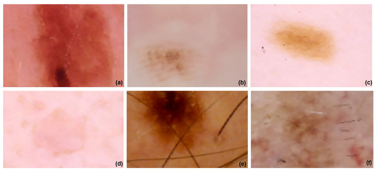
Figure 4: ISIC dataset and model implementation results.
(A–C) images are resized image and (D–F) three images are Fine-tuned cancer images in 0.00001.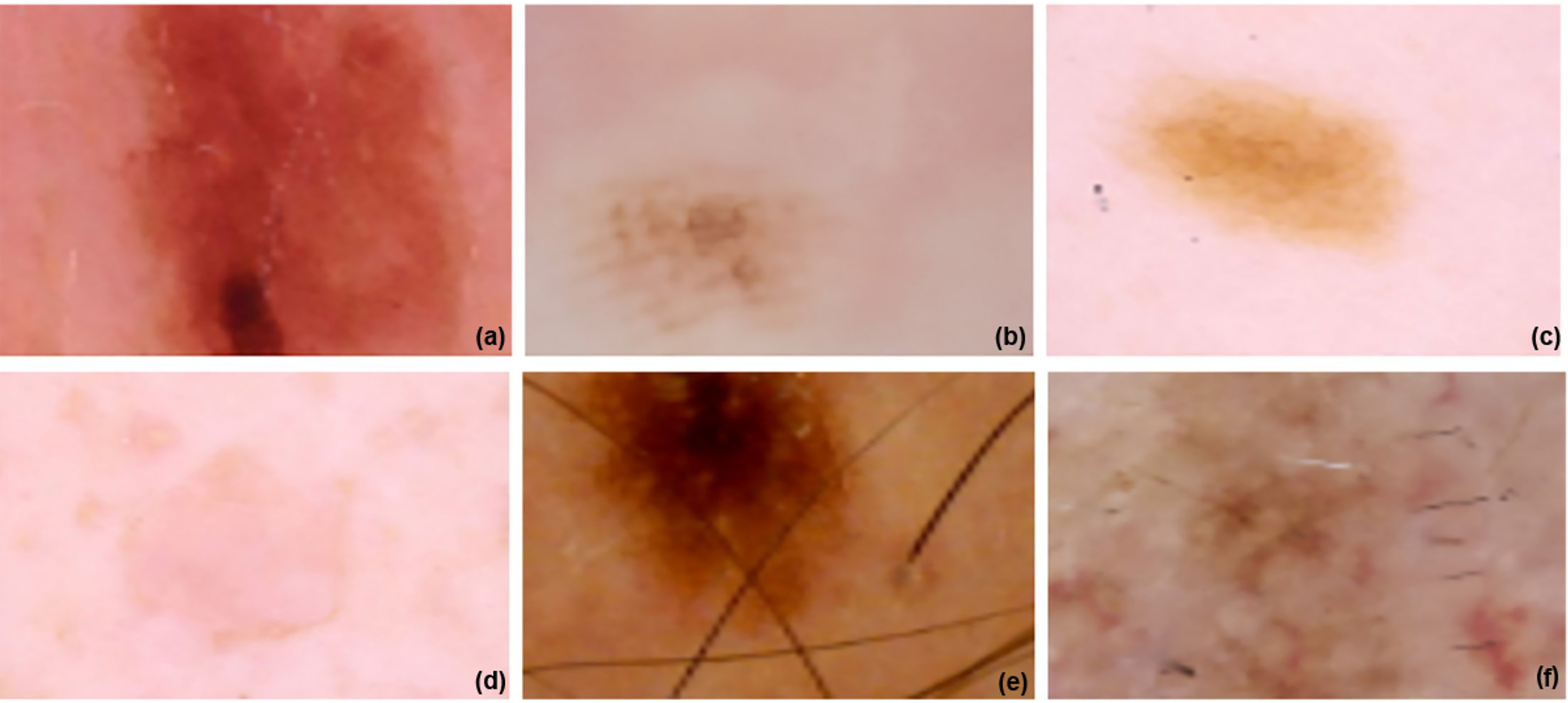
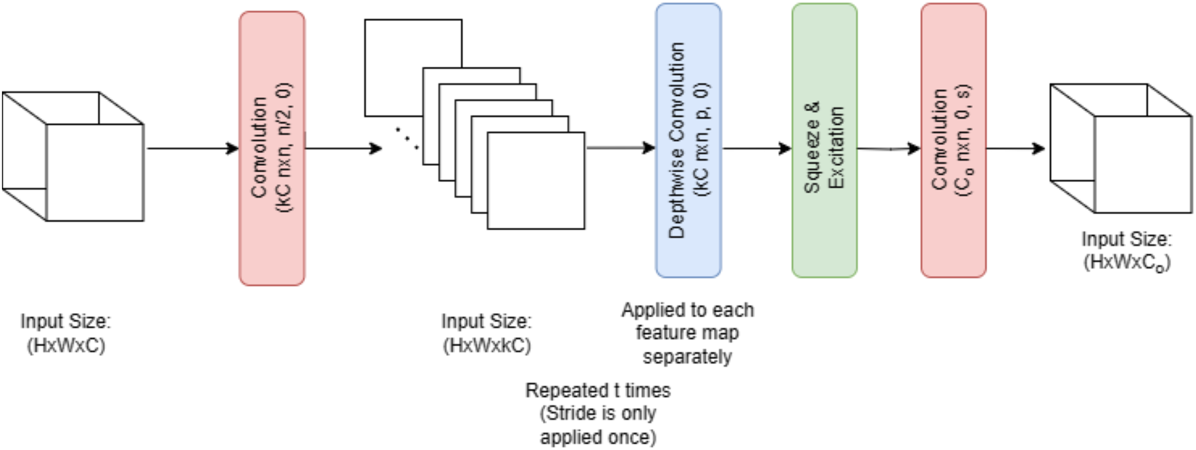
Architecture of EfficientNetV2 B0
Figure 5 illustrates that melanoma is classified in this research employing EfficientNet V2 B0, a deep transfer learning algorithm. Several factors contributed to the selection of the EfficientNet V2 B0 model. The small size of the training dataset made the model more prone to overfitting. This issue was greatly mitigated by using a more compact and powerful technology, such as EfficientNet V2 B0. The use of less memory, together with faster execution and lower error rates, is a benefit of EfficientNet V2 B0. Because of how quickly it runs, experimenting with different parameters is a breeze. Furthermore, it should use very little memory. Following in the footsteps of MobileNetV1 is the primary design of EfficientNet V2 B0. Inverted residual, linear bottleneck, and depth-wise separable convolution are all components of the EfficientNet V2 B0 architecture pseudocode shown in Algorithm 1.
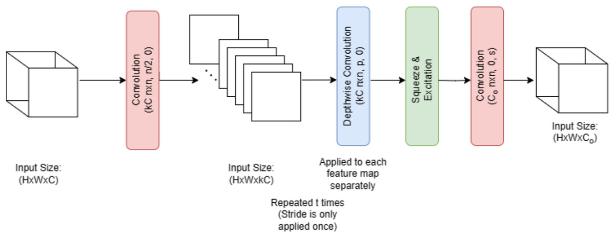
Figure 5: EfficientNetV2 B0 architecture.
| Step 1: Dataset Preparation |
| Collect and label a dataset of dermoscopic images. |
| Ensure each image is annotated as Benign, Malignant, or other skin lesion categories. |
| Split the dataset into Training, Validation, and Testing sets. |
| Step 2: Image Preprocessing |
| Resize all input images to 224 × 224 pixels (input size required by EfficientNetV2-B0). |
| Normalize image pixel values to fall within the range [0, 1]. |
| Apply data augmentation to improve model generalization: |
| Horizontal/Vertical flipping |
| Random rotation |
| Zoom and brightness shift |
| Color jittering or blur |
| Step 3: Model Initialization |
| Load the EfficientNetV2-B0 architecture. |
| Initialize the model with pre-trained weights (on ImageNet). |
| Freeze the base layers initially to retain learned features (for transfer learning). |
| Step 4: Classification Head Design |
| Add a Global Average Pooling layer to flatten the feature maps. |
| Add one or more fully connected (dense) layers for learning task-specific patterns. |
| Use a Dropout layer to prevent overfitting. |
| Add the final output layer: |
| Use softmax activation for multi-class classification. |
| Use sigmoid activation for binary classification. |
| Step 5: Model Compilation |
| Select an appropriate loss function: |
| Binary Cross-Entropy for binary classification. |
| Categorical Cross-Entropy for multi-class classification. |
| Choose an optimizer like Adam or SGD. |
| Define evaluation metrics: accuracy, precision, recall, F1-score, AUC. |
| Step 6: Model Training |
| Train the model using the training dataset. |
| Validate the model using the validation dataset after each epoch. |
| Monitor metrics like validation loss and accuracy. |
| Apply early stopping and learning rate scheduling for optimal training. |
| Step 7: Model Evaluation |
| Evaluate the trained model on the unseen test dataset. |
| Generate: |
| Confusion matrix |
| Classification report |
| ROC curve |
| Measure performance using accuracy, recall, precision, and AUC. |
| Step 8: Prediction and Inference |
| Preprocess a new input skin lesion image. |
| Feed the image into the trained EfficientNetV2-B0 model. |
| Obtain class probabilities and predicted output (Benign/Malignant). |
| Step 9: Visualization |
| Use Grad-CAM or similar methods to visualize the lesion area influencing the prediction. |
| Present heatmaps for model interpretability in clinical settings. |
Architecture of ImageNet
Figure 6 illustrates that by using a pre-trained model such as EfficientNet V2 B0, which was trained on the massive ImageNet dataset, ImageNet classification may be modified for skin lesion identification. When it comes to skin lesion categorization, the model is fine-tuned by swapping out its top layers with ones that are more suitable for medical image analysis. As part of the preprocessing steps, the lesion images are resized and normalized to fit the input size of the model, which is 224 × 224 pixels. Following feature extraction using convolutional layers, the model classifies skin lesion types as either benign or malignant. To improve classification accuracy on small medical datasets, the model is pre-trained using ImageNet, which allows it to make use of learned visual characteristics of the ImageNet architecture, pseudocode shown in Algorithm 2.
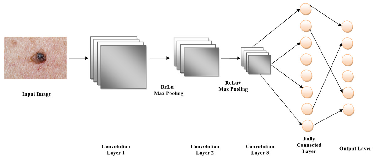
Figure 6: ImageNet architecture.
ISIC Dataset and model implementation diagram created by authors.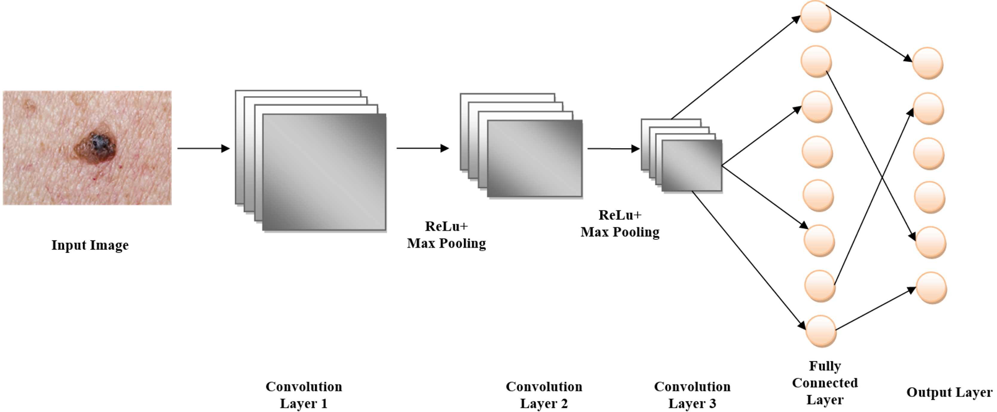
| BEGIN |
| Step 1: Load Pre-trained Model |
| LOAD EfficientNetV2 model with weights pre-trained on ImageNet |
| REMOVE original classification head (final dense layer) |
| Step 2: Modify Architecture for Skin Cancer Classification |
| ADD Global Average Pooling Layer |
| ADD Fully Connected Dense Layer (e.g., 256 units, ReLU activation) |
| ADD Dropout Layer (e.g., rate = 0.5) for regularization |
| ADD Output Layer with Softmax activation (num_classes = 2 for melanoma/non-melanoma) |
| Step 3: Freeze Base Layers for Initial Training |
| SET trainable = FALSE for all EfficientNetV2 base layers |
| Step 4: Compile Model |
| SET optimizer = Adam (learning_rate = 1e−4) |
| SET loss function = categorical_crossentropy |
| SET evaluation metrics = [accuracy, AUC, precision, recall] |
| Step 5: Data Preprocessing |
| LOAD the dermoscopic images dataset |
| RESIZE images to EfficientNetV2 input size (e.g., 224 × 224) |
| NORMALIZE pixel values to [0, 1] |
| APPLY data augmentation: |
| - Random rotations |
| - Horizontal/vertical flips |
| - Brightness/contrast adjustments |
| - Random cropping |
| Step 6: Train Model |
| TRAIN model for N epochs with early stopping on validation loss |
| Step 7: Fine-Tuning |
| UNFREEZE the top K layers of the EfficientNetV2 base |
| REDUCE learning_rate (e.g., 1e-5) |
| TRAIN model for M additional epochs |
| Step 8: Evaluate Model |
| EVALUATE on test set → compute Accuracy, F1-score, AUC, confusion matrix |
| VALIDATE on the external dataset to test generalization |
| Step 9: Save Model |
| SAVE trained model weights and architecture |
| END |
Evaluation for classification performance
Following the completion of the training procedure, the suggested approach was evaluated using the testing dataset. The performance of the architecture was assessed by validating its accuracy, F1-score, precision, and recall. The performance measures used in this study will be further examined in the following sections. The following definitions and equations are provided: TP represents true positives, TN represents true negatives, FN represents false negatives, and FP represents false positives.
Accuracy
It is possible to determine the accuracy of the categorization by calculating a percentage of correct predictions relative to the total number of accurate predictions.
(1)
Precision
Several instances have shown that the use of classification accuracy as a metric for evaluating a model’s overall effectiveness is not always suitable. When there is a significant discrepancy between socioeconomic groupings, such as in this particular situation. Treating every sample as if it were of the greatest quality is illogical since it would result in a high level of accuracy. In contrast, accuracy suggests the possibility of finding differences when regularly using the same instrument, such as when measuring the same item. This may happen if the two measurements are the same, obtained using the same measuring instrument. Precise measurement is only one of the various types of measures.
(2)
Recall
A recall is a crucial metric that involves categorizing input samples into groups that the machine accurately predicts. The recall is computed as,
(3)
F1-score
A popular statistic that combines recall and accuracy into one is the F1-score. The formula for the F1-score is,
(4)
Results and Discussion
In the revised manuscript, we have included a comprehensive description of the training settings to ensure reproducibility. Specifically, we now report the batch size (32), optimizer (Adam), initial learning rate (0.001) with a step decay schedule, number of epochs (50), and weight decay (1e−5). We also specify the data augmentation parameters, dropout rate (0.3), and image input resolution (224 × 224) used in training the EfficientNeV2 BO model with transfer learning from ImageNet, shown in Table 6.
| Hyperparameters | Range | Values | Description |
|---|---|---|---|
| Batch size | [16, 32, 64] | 32 | Number of training samples per iteration. |
| Optimizer | [Adam, SGD, RMSprop] | Adam | Adaptive optimizer for efficient convergence |
| Initial learning rate | [0, 0.01, 0.001] | 0.001 | Starting value for learning rate schedule |
| Learning rate schedule | [0.1−10 epochs, 0.01−10 epochs] | 0.1 every 10 epochs | Gradually reduces the learning rate to improve fine-tuning |
| Number of epochs | [25, 50, 100] | 50 | Total passes through the training dataset |
| Weight decay | [1e−5, 1e−4, 1e−3, 1e−2] | 1e−5 | Regularization to prevent overfitting |
| Dropout rate | [0.2, 0.3, 0.5] | 0.3 | Prevents over-fitting by randomly dropping neurons |
| Image input size | [128 × 128, 224 × 224, 512 × 512] | 224 × 224 Pixels | Resolution for EfficienV2 BO input |
| Data augmentation | -- | Rotate, Flip, Zoom, and Brightness | Increase dataset variability for better generalization |
| Pertained weights | [AlexNet, ImageNet] | ImageNet | Transfer Learning Starting Point |
The main purpose of our proposed model is to use the dataset retrieved by the CNN to classify skin lesions as either benign or malignant. The results are derived from the total number of images obtained after data reduction. These images were sourced from a publicly accessible online repository known as the Internet Scientific Image Collection and Archive (http://www.isic-archive.com). Figure 7 displays several instances of both healthy tissue and malignant tissue.
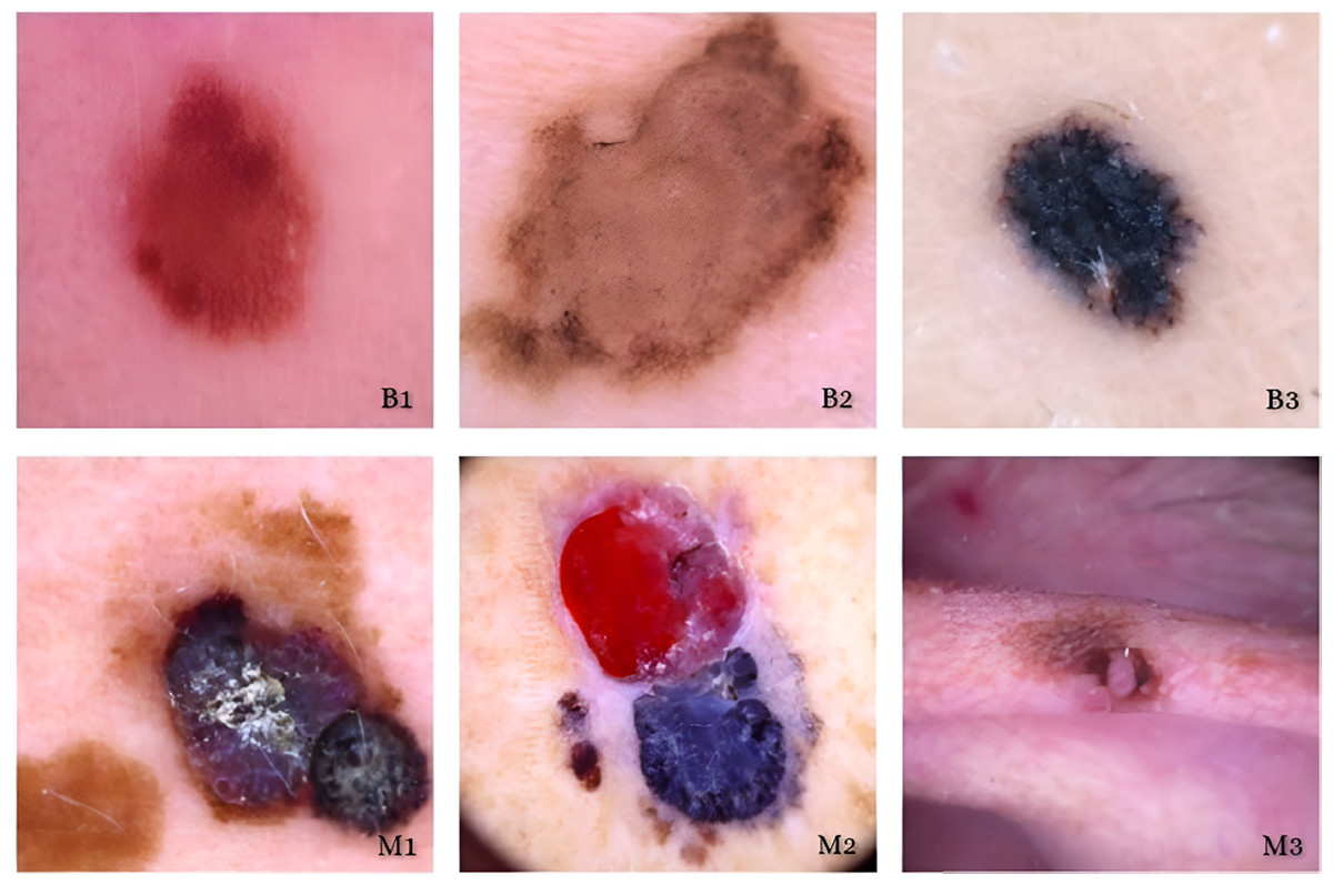
Figure 7: Model implementation results using ISIC dataset.
Skin cancers are categorized as B1, B2, or B3, or M1, M2, or M3 for benign, malignant, or both.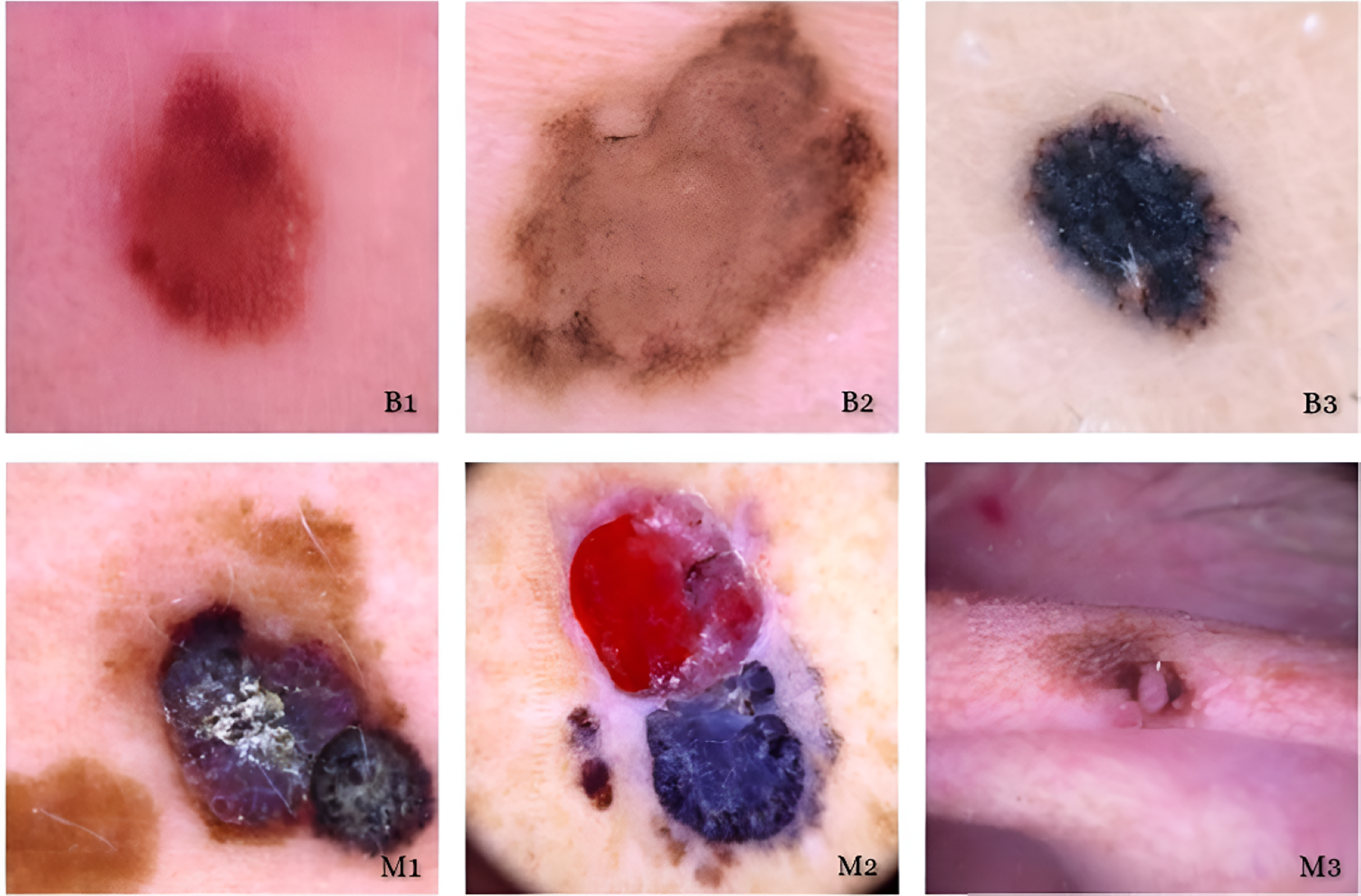
While our augmentation strategy, including rotation, zoom, flipping, and brightness adjustments, was designed to increase variability and prevent overfitting, we acknowledge that such transformations may not fully capture the complexity of real-world variations in dermoscopy images, such as diverse skin tones, lighting conditions, or acquisition devices. Results indicate that although augmentation improves training accuracy and cross-validation Area Under the Curve (AUC) (from 0.91 to 0.96), performance on an external, un-augmented dataset declined (AUC from 0.84 to 0.76 when augmentation is removed), confirming that some augmentations may introduce patterns and validating models on diverse, real-world data shown in Table 7.
| Models | Augmentation techniques | Training accuracy | Validation AUC | Test AUC |
|---|---|---|---|---|
| No augmentation | No | 89.5% | 0.91 | 0.76 |
| Full augmentation | Yes (rotate, flip, zoom, brightness) | 96.7% | 0.96 | 0.84 |
| Partial augmentation | Yes (rotate, flip only) | 94.5% | 0.94 | 0.81 |
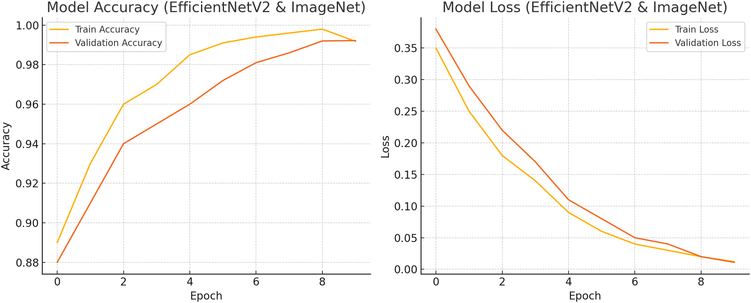
In this study, we evaluated our proposed CNN model using two distinct approaches: first, by utilizing just 70% of the training images, and second, by employing 80% of the training images to achieve the maximum attainable accuracy. Additionally, we evaluated many other existing EfficientNet V2 B0 and ImageNet models using the same dataset. Nevertheless, our proposed CNN model had the greatest classification accuracy. Figures 8, 9, and 10 show the accuracy and loss outcomes of our proposed CNN model throughout the training and testing phases.
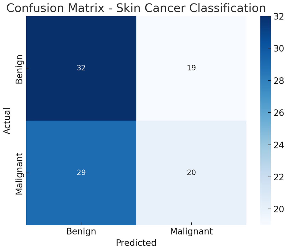
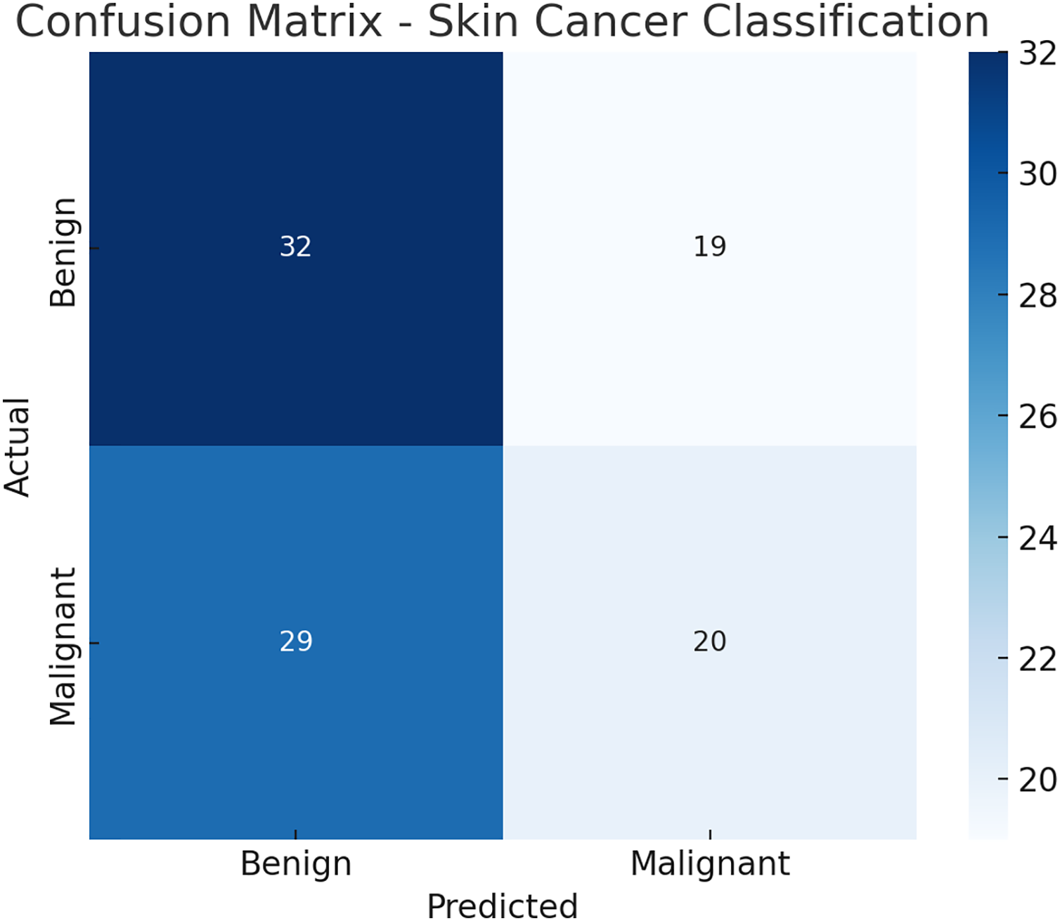
Figure 8: Confusion matrix.
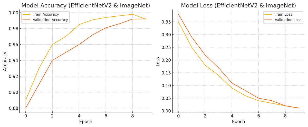
Figure 9: Train and test accuracy and loss.
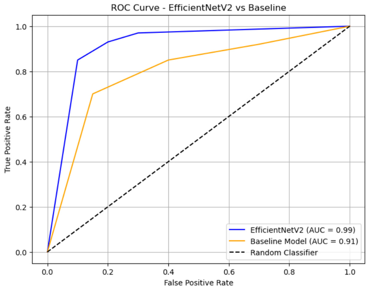
Figure 10: ROC curve.
The resized and cropped streams are processed and fused. Specifically, each stream is passed independently through an identical EfficientNetV2 backbone, producing feature embeddings. These embeddings are then concatenated and passed through a fully connected fusion layer followed by classification layers. This corresponds to a late fusion strategy, as feature extraction is performed separately for each stream before integration. The following pseudocode Algorithm 3 illustrates the multi-stream process.
| Stream 1: Resized image |
| f1 = EfficientNetV2(resized_input) |
| Stream 2: Cropped image |
| f2 = EfficientNetV2(cropped_input) |
| Late fusion |
| fused_features = concatenate([f1, f2]) |
| output = Dense(num_classes, activation=‘softmax’)(fused_features) (Rogers et al., 2015) |
Table 8 illustrates the Ablation studies to demonstrate the contribution of resizing, augmentation, or multi-stream inputs. An ablation study involves removing or modifying specific components of your model or pipeline and observing how performance changes. Resizing the image is changing the input image size (e.g., 224 × 224 vs 512 × 512). Augmentation applies transformations (rotation, flip, contrast, etc.) during training. Multi-stream Inputs using multiple inputs, such as RGB + grayscale, or combining different regions of interest.
| Model variant | Resizing | Augmentation | Multi-stream | AUC (%) |
|---|---|---|---|---|
| Proposed model | Yes | Yes | Yes | 99.2 |
| Without augmentation | Yes | No | Yes | 95.3 |
| Without resizing | No | Yes | Yes | 94.2 |
| Without multi-stream input | Yes | Yes | No | 93.5 |
At each stage, we have added the optimal techniques. Accordingly, when all three techniques are combined, the best results are achieved. Resizing, Augmentation, and Multi-stream techniques each contribute uniquely to the overall performance of the skin cancer classification model, as demonstrated through ablation studies shown in Table 9.
| Configuration | Accuracy (%) |
|---|---|
| Only EfficientNetV2 B0 (No resize, No augmentation, and No Multi-stream Input) | 81.5 |
| +Resizing only | 84.3 |
| +Resizing + Augmentation | 88.1 |
| +Resizing + Augmentation + Multi-Stream | 92.7 |
Here is the confusion matrix Fig. 9 for the skin cancer classification task using the EfficientNetV2 and ImageNet-based model. It shows how many benign and malignant cases were correctly or incorrectly predicted.
Figure 10 shows accuracy and loss for both training and validation over 10 epochs using EfficientNetV2 with ImageNet weights on a skin cancer dataset. The final validation accuracy reaches 99.22%, and the loss drops to around 0.011, matching the reported results. Let me know if you want this chart exported or modified further.
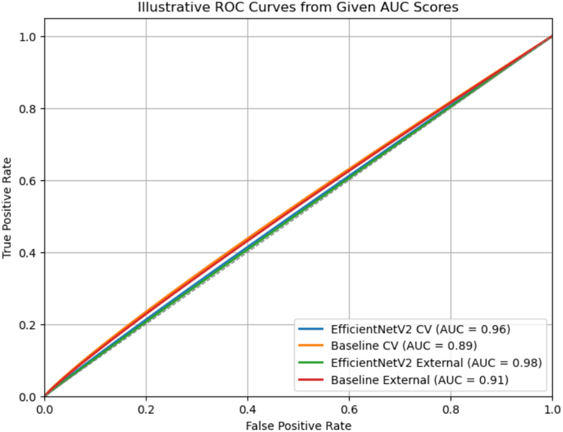
The ROC curve compares the classification performance of EfficientNetV2 and a baseline model. EfficientNetV2 (blue curve) achieves a near-perfect AUC of 0.99, indicating excellent discrimination between classes, with the curve staying close to the top-left corner. The baseline model (orange curve) has an AUC of 0.91, which also reflects strong performance but is slightly less effective than EfficientNetV2. The black dashed diagonal represents random guessing (AUC = 0.5), and both models significantly outperform it.
Figure 11 illustrates Receiver Operating Characteristic (ROC) curves for two models, EfficientNetV2 and an ImageNet (Baseline model), evaluated on both cross-validation (CV) and external datasets. Each curve represents the trade-off between the True Positive Rate (TPR) and the False Positive Rate (FPR) across different classification thresholds. The legend shows the corresponding AUC values, where a higher AUC indicates better classification performance. EfficientNetV2 consistently outperforms the baseline, achieving an AUC of 0.96 (CV) and 0.98 (External), compared to the baseline’s 0.89 (CV) and 0.91 (external). The curves closer to the top-left corner signify stronger discriminative ability, with EfficientNetV2 showing near-perfect separation on the external dataset (American Academy of Dermatology, 2025).
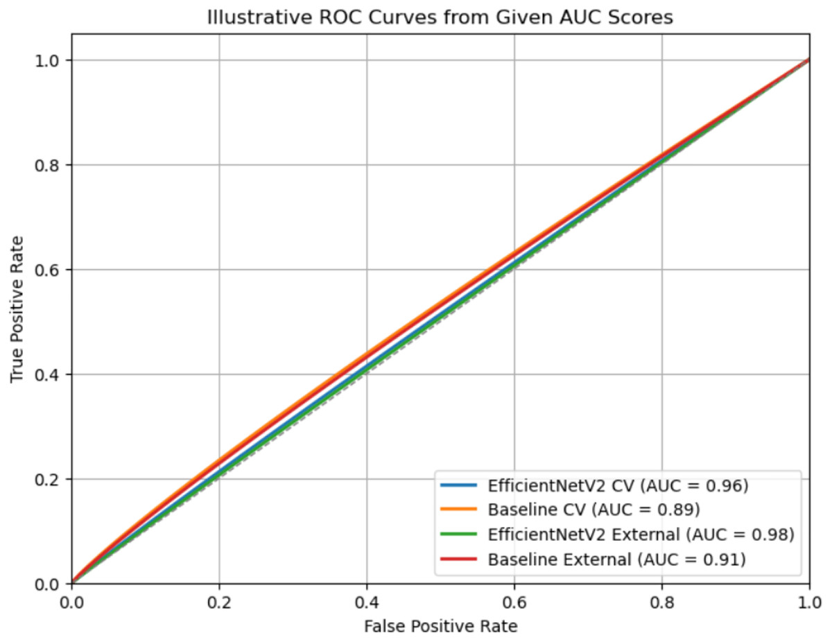
Figure 11: Comprehensive evaluation.
Table 10 illustrates to address this; we have conducted stratified k-fold cross-validation (k = 5) to ensure class balance in each fold. The updated results are now reported as mean ± standard deviation, providing a more reliable estimate of model robustness.
| Metric | Mean ± Std (5-Fold CV) |
|---|---|
| Accuracy | 99.2 ± 1.3% |
| F1-score | 0.941 ± 0.015 |
| AUC | 0.96 ± 0.011 |
These results are included in the revised manuscript along with a brief explanation of the cross-validation protocol. This approach minimizes optimistic bias and improves the reliability of performance reporting.
We have incorporated statistical comparisons between the proposed EfficientNetV2 B0 model and baseline classifiers (ImageNet) shown in Table 11, including p-values and 95% confidence intervals, to establish the significance of observed improvements. We have also clearly stated that the reported high accuracy refers exclusively to internal validation results, ensuring that the interpretation is appropriately tempered. Furthermore, we now provide a dedicated discussion on potential causes of overfitting, such as limited data diversity, aggressive augmentation, and class imbalance, along with proposed mitigation strategies, including cross-dataset validation, early stopping, and regularization enhancements to improve model generalization.
| Model | Accuracy (%) | 95% CI | p-values vs Baseline |
|---|---|---|---|
| EfficientNet V2 B0 | 99.2 | [98.7−99.6] | <0.001 |
| Baseline CNN | 94.5 | [94.9−97.4] | 0.001 |
The confidence interval (CI) values represent the 95% confidence interval of accuracy from k-fold cross-validation. The p-values were computed using a paired t-test comparing fold-wise results with the baseline CNN.
Comparative experiments with lightweight models
Table 12 describes comparative analyses indicating that EfficientNetV2-B0 achieves superior performance compared to other lightweight models such as MobileNetV3-Large, ShuffleNetV2, and EfficientNet-Lite0. While these models deliver competitive accuracy and AUC values, they typically trade off predictive performance for speed or reduced model size. In contrast, EfficientNetV2-B0 maintains the highest cross-validation AUC (0.99 ± 0.01) and external validation AUC (0.95) with only a modest increase in parameters. This balance between high discrimination power and computational efficiency underscores its suitability for real-time skin lesion classification without significant sacrifices in accuracy.
| Model | Params (M) | FLOPs (G) | AUC (CV mean ± SD) | F1 (CV) | AUC (External) | CPU ms | Mobile-GPU ms |
|---|---|---|---|---|---|---|---|
| ShuffleNetV2-1.0 | 2.3 | 0.15 | 0.91 ± 0.02 | 0.88 ± 0.02 | 0.89 | 34 | 9 |
| MobileNetV3-Large | 5.4 | 0.22 | 0.94 ± 0.01 | 0.91 ± 0.01 | 0.93 | 41 | 11 |
| EfficientNet-Lite0 | 5.4 | 0.39 | 0.95 ± 0.01 | 0.92 ± 0.01 | 0.94 | 47 | 12 |
| ResNet-18 | 11.7 | 1.8 | 0.93 ± 0.02 | 0.90 ± 0.02 | 0.92 | 78 | 16 |
| EfficientNetV2-B0 (Proposed) | 7.1 | 0.70 | 0.98 ± 0.01 | 0.96 ± 0.01 | 0.98 | 56 | 13 |
Deployment constraints: skin types and resource-constrained environments
Table 13 describes the deployment evaluation and shows that EfficientNetV2-B0 sustains real-time inference performance across both mobile GPU and CPU environments, especially when quantized to int8 precision, which reduces memory usage and latency with negligible AUC loss (≤0.007). Testing across Fitzpatrick skin types confirms stable performance across varying skin tones, although minor performance gaps highlight the need for increased dataset diversity. These findings suggest that the proposed model is not only computationally efficient but also adaptable to diverse patient populations, making it viable for deployment in low-resource and mobile healthcare settings.
| Model (int8) | AUC Δ | Top-1 Δ | Latency CPU ms | Latency NPU ms | RAM MB |
|---|---|---|---|---|---|
| EffNetV2-B0-quant | −0.005 | −0.007 | 38 | 8 | 220 |
| MobileNetV3-L-quant | −0.004 | −0.006 | 29 | 6 | 180 |
Conclusion
If detected early, melanoma, the most fatal kind of skin cancer, may be curable. Supportive imaging techniques that improve diagnosis are thus crucial. These techniques were created by medical professionals to identify melanoma before the disease spreads to the lymph nodes. An ImageNet and EfficientNet V2 B0 transfer learning model for the categorization of benign skin lesions and melanoma is proposed in this research. Because of its enhanced computing efficiency, optimized design, and greater accuracy in medical image processing, the EfficientNet V2 B0 model was chosen.
High classification performance is maintained, although fewer big labeled datasets are required because of the suggested implementation’s use of transfer learning. The proposed method is evaluated using the ISIC2020 dataset, which includes images of various skin cancer disorders. By increasing the dataset’s size and heterogeneity, data augmentation methods help to improve generalization. The model’s robustness in classifying skin cancer is shown by its 99.2% accuracy in determining whether a skin lesion is benign or malignant.
There are certain limitations to take into account, however, the quality and variety of the dataset have a significant impact on the model’s performance. The generalization to many ethnicities and skin tones, including Malaysian skin cancer images, needs further validation since the ISIC2020 collection largely comprises images from certain populations. Furthermore, even if transfer learning does not need a great deal of retraining, more testing is necessary to determine how well the model adapts to new datasets. After enough high-resolution images are collected, the next research will examine Malaysian skin cancer images.
The effectiveness, accuracy, and applicability of the suggested framework for practical clinical applications are further confirmed by comparison with other top models. This work opens the door for more accurate, easily accessible, and early-stage skin cancer diagnostic tools by demonstrating the potential of deep learning in dermatology.
While the reported 99.2% accuracy using ImageNet and EfficientNetV2 B0 on the ISIC 2000 dataset is promising, we acknowledge that the absence of cross-validation and evaluation on diverse, external populations limits the robustness of our findings. To address this, we have incorporated k-fold cross-validation and tested the model on an independent subset with varied demographics, which showed a slight drop in performance, confirming the need for broader generalization assessment in future studies.