
Estimation of maize LCC and FVC for full growth periods based on UAV remote sensing and ensemble learning
- Published
- Accepted
- Received
- Academic Editor
- Consolato Sergi
- Subject Areas
- Artificial Intelligence, Computer Vision, Spatial and Geographic Information Systems, Theory and Formal Methods, Visual Analytics
- Keywords
- Vegetation index, Texture feature, Ensemble learning, Unmanned aerial vehicle remote sensing
- Copyright
- © 2025 Yao et al.
- Licence
- This is an open access article distributed under the terms of the Creative Commons Attribution License, which permits unrestricted use, distribution, reproduction and adaptation in any medium and for any purpose provided that it is properly attributed. For attribution, the original author(s), title, publication source (PeerJ Computer Science) and either DOI or URL of the article must be cited.
- Cite this article
- 2025. Estimation of maize LCC and FVC for full growth periods based on UAV remote sensing and ensemble learning. PeerJ Computer Science 11:e3356 https://doi.org/10.7717/peerj-cs.3356
Abstract
Fractional vegetation cover (FVC) and leaf chlorophyll content (LCC) are essential parameters that reflect crop growth. An empirical approach to estimating LCC and FVC involves analyzing vegetation index (VI) derived from crop canopy reflectance and integrating them with statistical regression methods. However, when estimating crop parameters throughout full growth periods, conventional single models frequently exhibit significant accuracy variations across different growth stages. To overcome this limitation, we introduced a novel phenology-adaptive framework using unmanned aerial vehicle (UAV) remote sensing and advanced ensemble learning (Stacking, Bagging, Blending) for maize monitoring. By synergistically integrating VI and texture features (TF) from UAV imagery as input variables, this study conducted the first systematic comparison of three ensemble models for estimating LCC and FVC. The estimation accuracy of VI, TF, and combined VI + TF inputs was rigorously evaluated. Notably, the Stacking model with VI + TF inputs achieved breakthrough performance: LCC (R2 = 0.945, root mean squared error (RMSE) = 3.701 Soil-Plant Analysis Development (SPAD) units, mean absolute error (MAE) = 2.968 SPAD units) and FVC (R2 = 0.645, RMSE = 0.045, MAE = 0.036), demonstrating >20% accuracy gain in early growth stages. This research successfully applied spectral, texture features, and ensemble learning to achieve high-precision estimation of LCC and FVC, providing a methodological reference for high-performance crop trait parameter estimation.
Introduction
Fractional vegetation cover (FVC) and leaf chlorophyll content (LCC) are critical parameters reflecting crop growth (Kovács et al., 2024; Hu et al., 2024). Accurate dynamic monitoring of LCC and FVC is beneficial for agricultural management, such as analyzing crop phenological stages or identifying environmental stress factors during the growth cycle (Chakhvashvili et al., 2022).
Traditional methods for monitoring LCC and FVC rely on destructive measurements that require considerable time and effort, making them unsuitable for wide-ranging LCC and FVC monitoring (Gée et al., 2021). Chlorophyll within green plant leaves acts as a catalyst, converting electromagnetic waves into chemical energy while absorbing red and blue light (Mandal & Dutta, 2020; Yue et al., 2023). As a result, crops exhibit a reflectance peak in the green wavelength range. Additionally, due to the multiple scattering effects of leaf mesophyll cells, green vegetation demonstrates very elevated reflectance within the near-infrared spectrum. The most distinct spectral differences between green vegetation and other earth surface features are these characteristics (Zeng et al., 2022). Thus, crop canopy spectral reflectance is closely associated with LCC and FVC, enabling dynamic monitoring through remote sensing technology (Abdelbaki & Udelhoven, 2022).
The radiative transfer model is constructed based on physical principles, such as geometric optical models and the PROSAIL model (Tomíček, Mišurec & Lukeš, 2021). However, its application is often constrained by the many required model parameters, which are challenging to obtain in practice, thereby limiting its practical utility (Boren & Boschetti, 2020). The empirical method for estimating LCC and FVC is to analyze vegetation index (VI) based on measured crop canopy reflectance and combine them with statistical regression methods. Commonly used regression techniques include Gaussian process regression (GPR), linear regression (LR), ridge regression (RR), random forest regression (RFR), support vector machine regression (SVR), and k-nearest neighbors regression (KNNR). For example, Ganeva et al. (2022) estimated wheat leaf area index (LAI) and LCC based on unmanned aerial vehicle (UAV) multispectral images, where GPR achieved the highest prediction performance, with (R2 = 0.48; RMSE = 0.64) for LAI, and (R2 = 0.49; RMSE = 31.57 mg m−2) for LCC. Jewan et al. (2024) evaluated the feasibility of remote sensing technology for estimating Bambara peanut’s aboveground biomass (AGB), with the multiple linear regression (MLR) model achieved the best performance (R2 = 0.77, RMSE = 0.30) on the testing dataset.
In recent years, UAV remote sensing has shown excellent agricultural monitoring and management potential due to its high efficiency, flexibility, and low cost (Zhang et al., 2021). UAVs outfitted with multispectral or high-resolution digital cameras can acquire high-resolution imagery over large farmland areas in a short period. UAVs often acquire high-resolution imagery, where TF can reflect crop LCC and FVC characteristics. Texture analysis techniques extract patterns, structures, and spatial distributions from canopy imagery, providing comprehensive insights into crop growth (Tan et al., 2021). For example, Marcone et al. (2024) developed an accurate and transferable machine learning model using UAV multispectral images to monitor and estimate garlic yield. The optimal results achieved by combining vegetation indices with texture features extracted from UAV images were (R2 = 0.93, RMSE= 19.81%). Yang et al. (2024) conducted real-time and non-destructive monitoring of millet AGB during critical growth stages using remote sensing data collected by multi-sensor UAV, with the Random Forest (RF) model exhibiting the best performance (R2 = 0.877, RMSE = 0.207 kg/m2).
UAV remote sensing offers distinct advantages over satellite platforms for agricultural monitoring at the field and plot scale. Gurdak et al. (2021) using Copernicus satellite products to compare crop growth conditions for maize and winter wheat in Poland and South Africa. These include unprecedented spatial resolution, high temporal flexibility allowing for near-real-time monitoring during critical growth windows regardless of satellite revisit cycles, and control over acquisition timing under optimal illumination conditions.
Machine learning models are among the most commonly used methods for the empirical estimation of LCC and FVC. Renowned for their powerful data processing capabilities and automatic feature extraction, machine learning has achieved significant advancements in agriculture (Saleem, Potgieter & Arif, 2021).
Alam et al. (2025) found machine learning (especially kernel ridge regression) outperformed hybrid physical models for canopy nitrogen estimation (R2 = 0.94), matched hybrid accuracy for chlorophyll (R2 ≤ 0.93), and refined the critical corn canopy nitrogen content conversion factor to 3.03 at Michigan’s Kellogg Biological Station. Moreover, another study (Alam et al., 2024) demonstrates that machine learning algorithms (MLRAs) applied to UAV-satellite data fusion significantly outperformed hybrid physical models in precisely mapping crop canopy chlorophyll at Michigan’s Kellogg Biological Station, with kernel ridge regression achieving R2 = 0.89 when fusing UAV and RapidEye data.
These models have been widely applied in crop disease identification (Li et al., 2020), vegetation classification (Zhang et al., 2021), ecological parameter monitoring (Ghannam & Techtmann, 2021; Yue et al., 2024), and phenological information extraction (Yao et al., 2024). Additionally, machine learning techniques have been extensively applied in combination with remote sensing for the estimation and analysis of crop parameters, including biomass, chlorophyll content, and LAI. However, the performance of machine learning models is highly dependent on large training datasets and complex hyperparameter tuning. When data are limited, the advantages of machine learning may not be fully realized (Ali et al., 2023). Moreover, numerous studies have demonstrated that single regression models often fail to fully leverage image features, resulting in limited model generalization and accuracy. Furthermore, when estimating crop parameters across the full growth periods, different models exhibit significant accuracy variations at various crop growth stages.
Ensemble learning refers to a machine learning approach that integrates multiple models to enhance the accuracy of predictions (Ganaie et al., 2022). Specifically, integrating multiple weak learners can result in the formation of a strong learner. Ensemble learning typically offers better generalization capability than individual models and reduces the risk of overfitting. Ensemble learning significantly enhances accuracy by effectively mitigating errors from individual models. This approach leverages the strengths of multiple models, compensating for the limitations of any single model and substantially improving overall performance (de Zarzà et al., 2023). Besides, ensemble learning demonstrates strong robustness. Single models are often sensitive to noise and outliers, which can result in unstable predictions. In contrast, ensemble models integrate results from multiple models, making them more resistant to noise and better suited for a broader range of applications. Therefore, ensemble learning models, which improve generalization ability and reduce the risk of overfitting, are particularly suitable for various machine learning tasks and application scenarios, especially for estimating crop parameters across the full growth periods in dynamic agricultural environments (Gharakhanlou & Perez, 2024).
This study integrates spectral and TF from UAV imagery as input variables to evaluate the feasibility of three ensemble learning models: Stacking, Bagging, and Blending for high-precision maize LCC and FVC estimation. The study focuses on three key aspects:
-
(1)
Conducting multispectral imagery acquisition and LCC, FVC data collection across full growth stages in a maize breeding experimental field.
-
(2)
Evaluating the potential of Stacking, Bagging, and Blending models for LCC and FVC estimation, specifically comparing the accuracy of VI, TF, and VI + TF as inputs.
-
(3)
LCC and FVC mapping was conducted based on the optimal estimation strategy, and the relationships between remote sensing estimated and field measured distributions of FVC and LCC were analyzed. The results obtained in this research provide methodological references for estimating crop trait parameters and advancing the application of remote sensing in agricultural monitoring.
Experimental area and data collection
Experiment and experimental area
The research was conducted in Xingyang City, located in Zhengzhou, Henan Province, China (Fig. 1), situated in central Henan Province near the central and lower sections of the Yellow River. The region experiences a warm temperate continental monsoon climate, with an annual average temperature of approximately 14.8 °C and an average annual precipitation of about 608.8 mm. The experimental data were collected at the breeding trial fields of Henan Jinyuan Seed Industry Co., Ltd. A total of 160 maize planting plots (10 rows × 16 columns) were selected for the study.
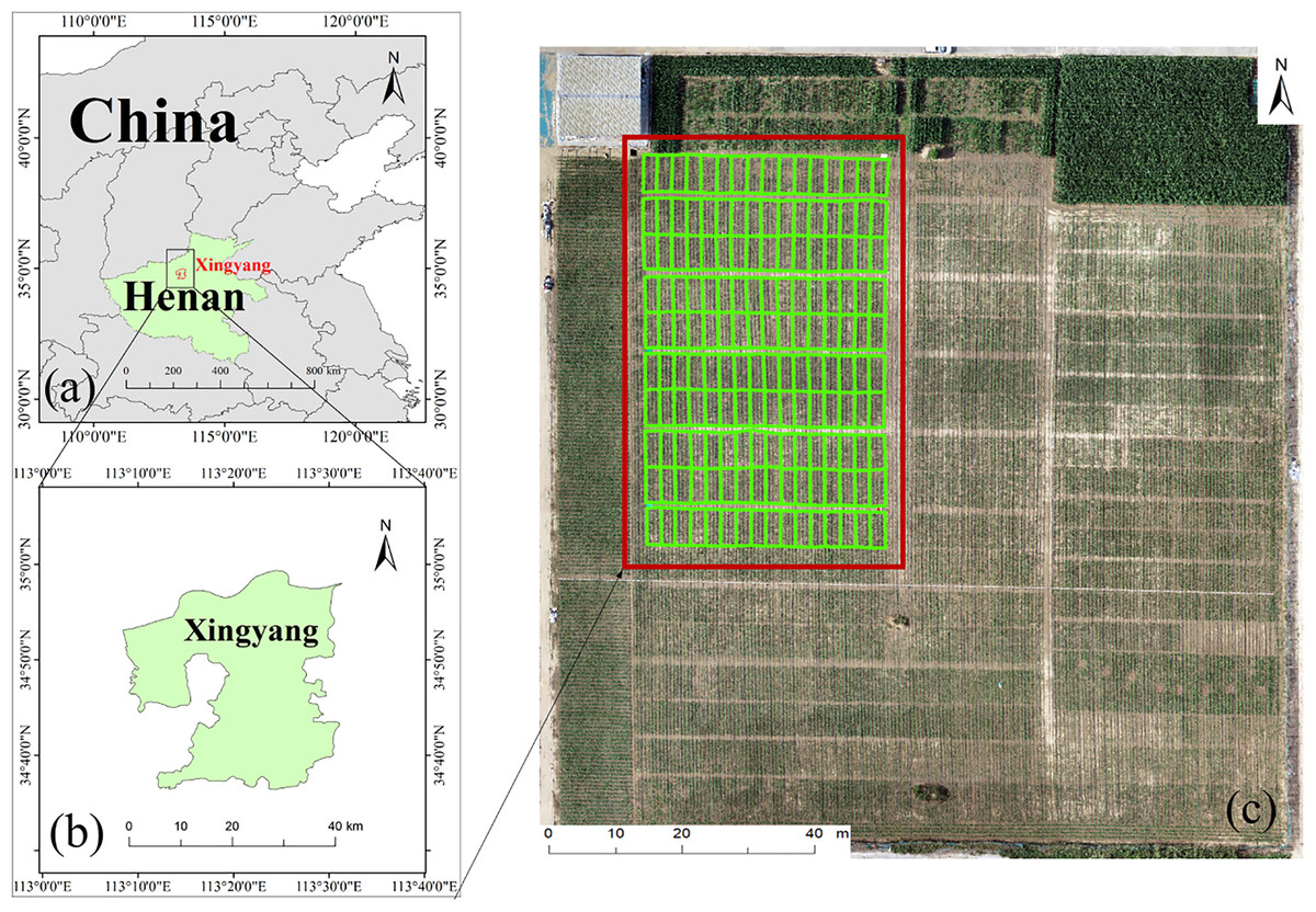
Figure 1: Overview of the experimental area and experimental field.
(A) Location of Henan Province, China; (B) Xingyang City; (C) experimental maize cultivation site.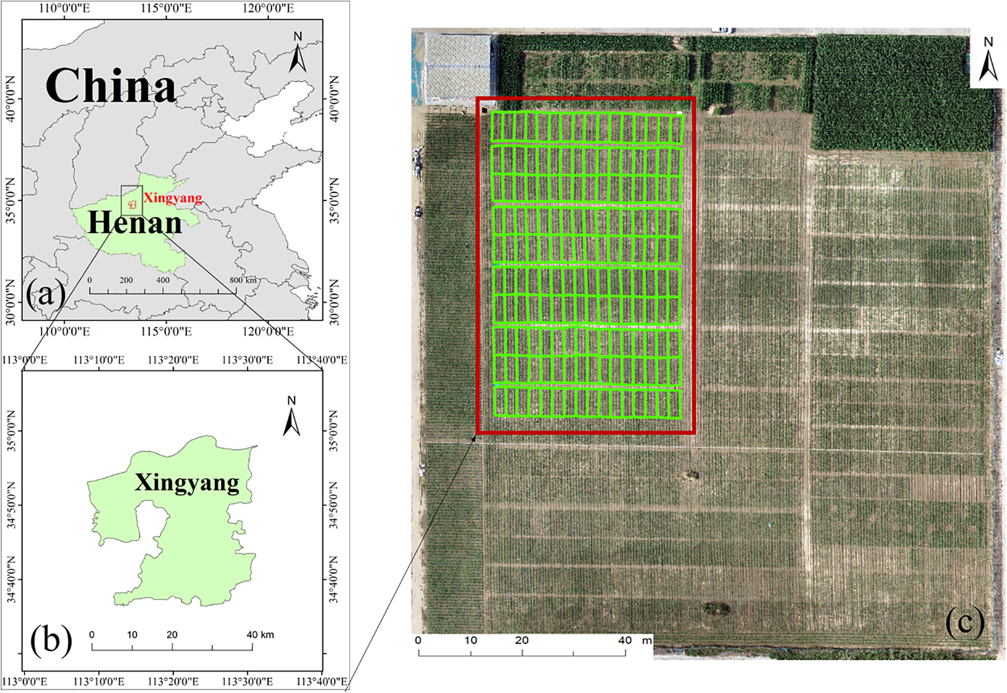
Data collection was conducted over 12 time points from the seedling stage to the tasselling stage of the maize breeding lines, covering the full growth periods. The specific dates for data collection were: 30 June (P1), 5 July (P2), 8 July (P3), 16 July (P4), 22 July (P5), 27 July (P6), 10 August (P7), 18 August (P8), 1 September (P9), 7 September (P10), 14 September (P11), and 21 September (P12).
UAV data collection
As the remote sensing platform, the DJI Phantom 4 multispectral UAV was employed in this study. Weighing 1,487 g, this UAV is equipped with six camera sensors, each featuring a 1/2.9″ size. The monochrome sensors capture data in five bands: red (R), green (G), blue (B), red-edge (RE), and near-infrared (NIR). Considering the endurance capacity of small UAVs and their flight safety, the DJI Phantom 4M flight height was set to 20 m.
Data acquisition with the UAV was conducted under stable solar radiation conditions on clear, cloudless days between 10:00 and 14:00. The longitudinal overlap was adjusted to 80%, the lateral overlap was fixed at 75%. The UAV followed preprogrammed flight paths and settings for automatic image data acquisition.
Field LCC and LAI measurement
Field measurements included LAI and LCC. The LAI was measured using an LAI-2200C Plant Canopy Analyzer. LCC was measured using a portable SPAD-502 sensor. It is important to note that adjacent maize planting plots were sown with the same maize inbred lines under identical growing conditions. Therefore, measurements of physiological traits were taken in just one plot from each pair. In each growth stage, data were collected from 80 maize plots. The results of the field measurements are shown in Table 1.
| Period | LCC (Soil-Plant Analysis Development (SPAD) units) | LAI | |||||||
|---|---|---|---|---|---|---|---|---|---|
| Num | Max | Min | Mean | Num | Max | Min | Mean | ||
| P1(6.30) | S1 | — | — | — | — | — | — | — | — |
| P2(7.05) | — | — | — | — | — | — | — | — | |
| P3(7.08) | 80 | 59.30 | 40.40 | 51.20 | — | — | — | — | |
| P4(7.16) | 80 | 54.10 | 43.40 | 54.30 | 80 | 3.88 | 1.19 | 2.80 | |
| P5(7.22) | 80 | 62.00 | 45.60 | 52.60 | 80 | 3.91 | 1.91 | 2.96 | |
| P6(7.27) | 80 | 61.50 | 47.40 | 53.98 | 80 | 4.17 | 2.21 | 3.11 | |
| P7(8.10) | S2 | 80 | 66.70 | 54.00 | 60.87 | 80 | 5.46 | 2.70 | 3.87 |
| P8(8.18) | 80 | 69.30 | 53.90 | 60.57 | 80 | 5.90 | 2.14 | 3.62 | |
| P9(9.01) | S3 | 80 | 64.20 | 28.90 | 47.60 | 80 | 6.78 | 2.05 | 4.13 |
| P10(9.07) | 80 | 53.60 | 18.30 | 38.75 | 80 | 4.81 | 1.10 | 2.91 | |
| P11(9.14) | 80 | 47.80 | 17.60 | 31.01 | 80 | 5.33 | 0.85 | 2.73 | |
| P12(9.21) | 80 | 40.20 | 11.50 | 22.43 | — | — | — | — | |
| Total | 800 | 69.30 | 11.50 | 47.33 | 640 | 6.78 | 0.85 | 3.27 | |
Note:
For periods P1 to P3, the maize plants were small, and measurements were not conducted. The unmeasured data is marked as “—”. The maize LCC and FVC samples were categorized by month as follows: S1, S2, and S3.
The LAI was transformed into FVC according to the equation presented below Eq. (1) (Nilson, 1971; Song et al., 2017):
(1)
In the equation, G represents the spherical orientation of the leaf projection factor, ϴ denotes the solar zenith angle, and Ω corresponds to the aggregation index (G = 0.5, ϴ = 0, Ω = 1). The observations in this research were conducted within a suitable time window (12:00—12:30), during which the variation in solar zenith angle was limited. Approximating it as a constant ensures the accuracy and consistency of the results.
In the experiment, we measured LCC and LAI values in each maize planting plot. These ground-truth measurements were then compared with the remotely estimated LCC and FVC values to ensure a comprehensive machine learning modeling approach (Bochenek et al., 2017).
Method
Methodological framework
The methodological framework for this study is illustrated in Fig. 2. It illustrates the estimation methods for LCC and FVC parameters, as detailed below: (1) Data analysis and cleaning of field measured LCC and LAI were performed to remove errors or outliers, followed by converting LAI into FVC. Preprocessing of UAV multispectral images was conducted, including image stitching and calibration. (2) VI calculation and TF extraction were performed on the preprocessed UAV multispectral images. Correlation analysis was carried out separately for LCC and FVC, focusing on the relationship between VI and TF. (3) Different features (VI, TF, VI+TF) were input into various regression models to evaluate the estimation performance. (4) The optimal estimation strategy was selected for the visualization and mapping of LCC and FVC.
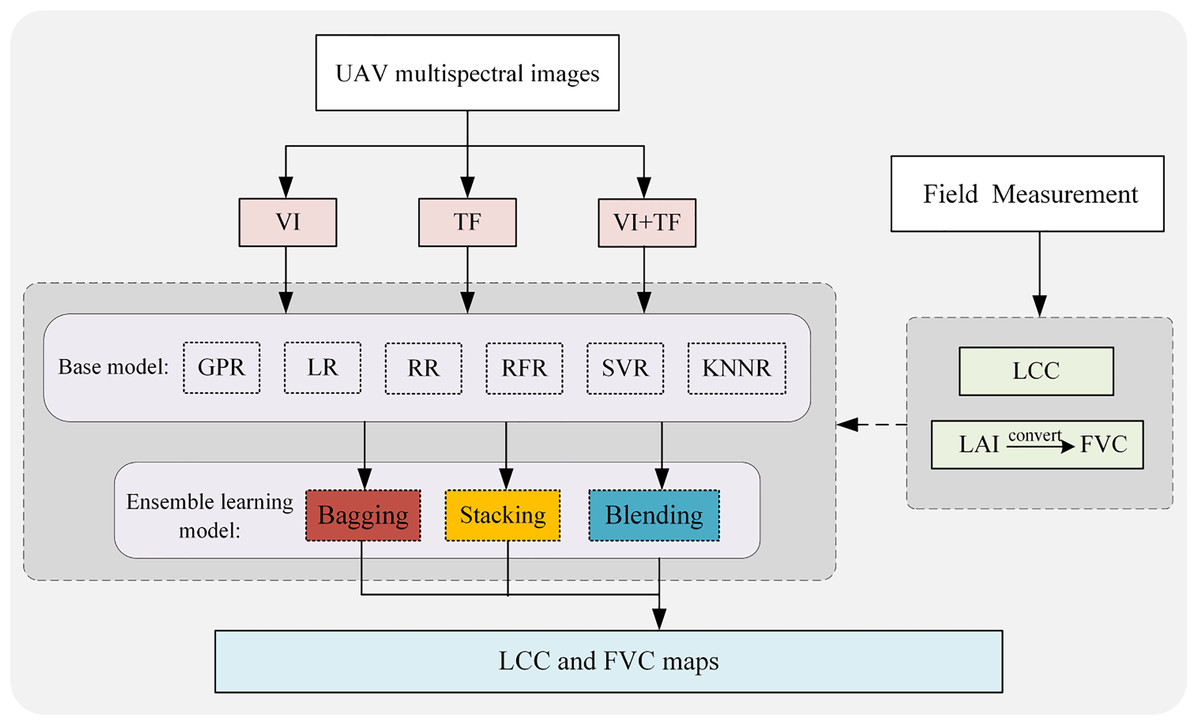
Figure 2: Methodological framework.
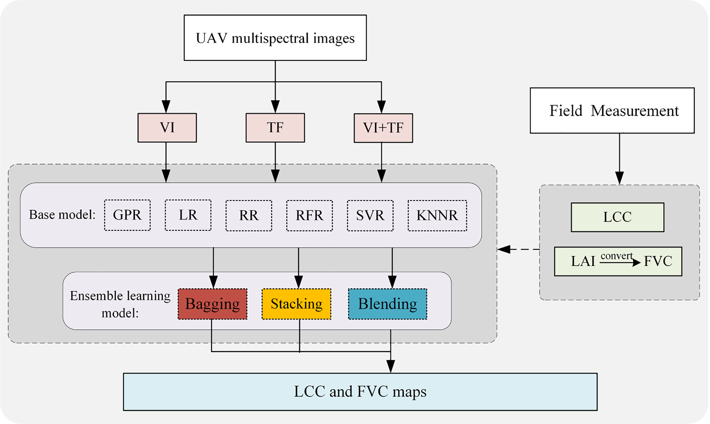
Vegetation index features
VI primarily reflect the difference in reflection between vegetation in the visible and near infrared bands and the soil background, and they can be used to quantitatively describe the growth status of vegetation (Neinavaz et al., 2021; Yue et al., 2023). In this study, five commonly used VIs were selected for estimating LCC and FVC in maize, namely the green normalized difference vegetation index (GNDVI), leaf chlorophyll index (LCI), normalized difference red edge (NDRE), normalized difference vegetation index (NDVI), and optimized soil adjusted vegetation index (OSAVI). The detailed calculation equations are provided in Table 2.
| Abbreviation | Name | Calculation | Reference |
|---|---|---|---|
| NDVI | Normalized difference vegetation index | (NIR − R)/(NIR + R) | Song et al. (2017) |
| NDRE | Normalized difference red edge | (NIR − RE)/(NIR + RE) | Bochenek et al. (2017) |
| LCI | Leaf chlorophyll index | (NIR − RE)/(NIR + R) | Neinavaz et al. (2021) |
| OSAVI | Optimized soil adjusted vegetation index | 1.16(NIR − R)/(NIR + R + 0.16) | Yue et al. (2023) |
| GNDVI | Green normalized difference vegetation index | (NIR − G)/(NIR + G) | Rouse et al. (1974) |
Texture features
TFs are second order features that are not directly derived from the image but are first extracted into an intermediate matrix through computation, with statistical measures defined on it. TFs described the spatial color and intensity distribution of an image or its regions. TFs can represent the texture, structure, and spatial distribution of surface objects (León-Ecay et al., 2024). In this study, eight TFs were computed using the GLCM approach. Taking into account the maize cultivation conditions and the pixel resolution of the UAV images, a 3 × 3 window size was applied for the calculation of TFs. The specific calculation formulas are shown in Table 3.
| Name (Abbreviation) | Calculation |
|---|---|
| Mean (Mea) | |
| Variance (Var) | |
| Homogeneity (Hom) | |
| Contrast (Con) | |
| Dissimilarity (Dis) | |
| Entropy (Ent) | |
| Angular second moment (ASM) | |
| Correlation (Cor) |
Note:
i and j denote the row and column indices of the image, respectively; p (i, j) is the relative frequency of two adjacent pixels.
Ensemble learning and base regression models
Ensemble learning
Ensemble learning models, such as Stacking, Bagging, and Blending, aim to improve overall effectiveness by combining the predictions of multiple base regression models. These methods leverage the advantages of different models, while minimizing their specific limitations, demonstrating exceptional adaptability to diverse data types and complex problems (Rane et al., 2024). This makes ensemble learning particularly advantageous for challenging tasks, such as estimating LCC and FVC throughout the crop growth cycle.
The importance of employing ensemble learning models in this study cannot be overstated, particularly when dealing with the complex task of crop parameter estimation, where they demonstrate significant advantages. Although traditional single models can provide effective estimates in certain cases, they generally exhibit several limitations: First, single models struggle to fully capture the complex nonlinear relationships within the data. Second, they have poor robustness when faced with noise or outliers, which can lead to estimation errors. Finally, when training data is limited, single models are prone to overfitting, resulting in reduced predictive performance on new, unseen data. In contrast, ensemble learning models aggregate the predictions of multiple base learners, effectively combining the strengths of various models. This approach overcomes the shortcomings of individual models, enhancing overall predictive accuracy and stability.
Individual base learners often face significant limitations when estimating maize LCC and FVC for full growth periods. First, crops’ spectral and textural characteristics exhibit complex and dynamic changes during different growth stages (Guo et al., 2021; Yue et al., 2024). Single models frequently struggle to capture these nonlinear relationships effectively, leading to suboptimal predictive performance. For instance, variations in LCC and FVC typically follow intricate nonlinear patterns that are difficult for individual regression models to model accurately. Second, monitoring data are often noisy or contain outliers due to measurement errors, environmental changes, or sensor inaccuracies. Individual models generally lack robustness against such disturbances, reducing prediction reliability. Additionally, single models may perform well under specific conditions or during some growth stages but often need more generalization ability to achieve consistent performance across all crop growth stages. This lack of adaptability can lead to inconsistent results when applied to a full growth periods. Lastly, in scenarios involving high-dimensional feature spaces or limited training data, single models are prone to overfitting, where they capture noise rather than meaningful patterns, making them poorly suited for new, unseen data (Montesinos López, Montesinos López & Crossa, 2022).
Ensemble learning effectively addresses these issues by combining the outputs of multiple base learners through strategies such as voting, weighting, or stacking. By aggregating predictions, ensemble methods significantly improve model robustness, reducing sensitivity to noise and outliers. Furthermore, ensemble learning harnesses the complementary strengths of diverse models, allowing for a more comprehensive capture of the complex and nonlinear relationships inherent in crop growth data. This approach enables a finer-grained understanding of spectral and textural variations throughout the growth cycle. One of the key advantages of ensemble learning lies in its ability to balance bias and variance. By averaging or blending the predictions from multiple models, it mitigates the risk of overfitting while enhancing predictive accuracy (Shams et al., 2023). This characteristic is precious in agricultural monitoring, where data complexity and variability are often high. For tasks like LCC and FVC estimation, ensemble learning provides a more stable and reliable solution, effectively overcoming the limitations of single models.
In this study, three ensemble learning models Stacking, Bagging, and Blending were employed. These models integrated the following base learners: GPR, LR, RR, RFR, SVR, and KNNR, as illustrated in Fig. 2. For experimental validation, k-fold cross-validation was utilized. To prevent overfitting, L2 regularization was incorporated into the models.
Base regression models
The base regression models of the ensemble learning used in this study are GPR, LR, RR, RFR, SVR, and KNNR. GPR is a regression technique that does not rely on parameters and is founded on Bayesian inference. It uses Gaussian processes to model the pattern of the dependent variable, with advantages including non-parametric flexibility and uncertainty estimation (Rasmussen & Nickisch, 2010). LR is a method that models the relationship between independent and dependent variables using linear functions. The model adapts to the data by minimizing the squared residuals. It is a simple and intuitive model with limited capability for modeling complex nonlinear relationships (Su, Yan & Tsai, 2012). RR is a regularized form of linear regression that adds a regularization term to constrain the model parameters. It is beneficial for addressing collinearity (high correlation between features) (Hoerl & Kennard, 1970). RFR is an ensemble learning method that builds multiple decision trees and combines their predictions to perform regression tasks. It effectively reduces the risk of overfitting (Biau & Devroye, 2010). SVR is a regression analysis method based on SVM, widely used in machine learning and statistical modeling. The core idea of SVR is to maximize the model’s generalization ability for regression prediction, making it particularly suitable for high-dimensional and nonlinear data modeling. (Brereton & Lloyd, 2010). KNNR is an instance based supervised learning algorithm. It makes predictions by considering the similarity between data points and estimates the target value using nearby samples, making it particularly appropriate for handling nonlinear and multi-dimensional data (Song et al., 2017).
Results
Correlation analysis
Correlation analysis of vegetation indices with LCC and FVC
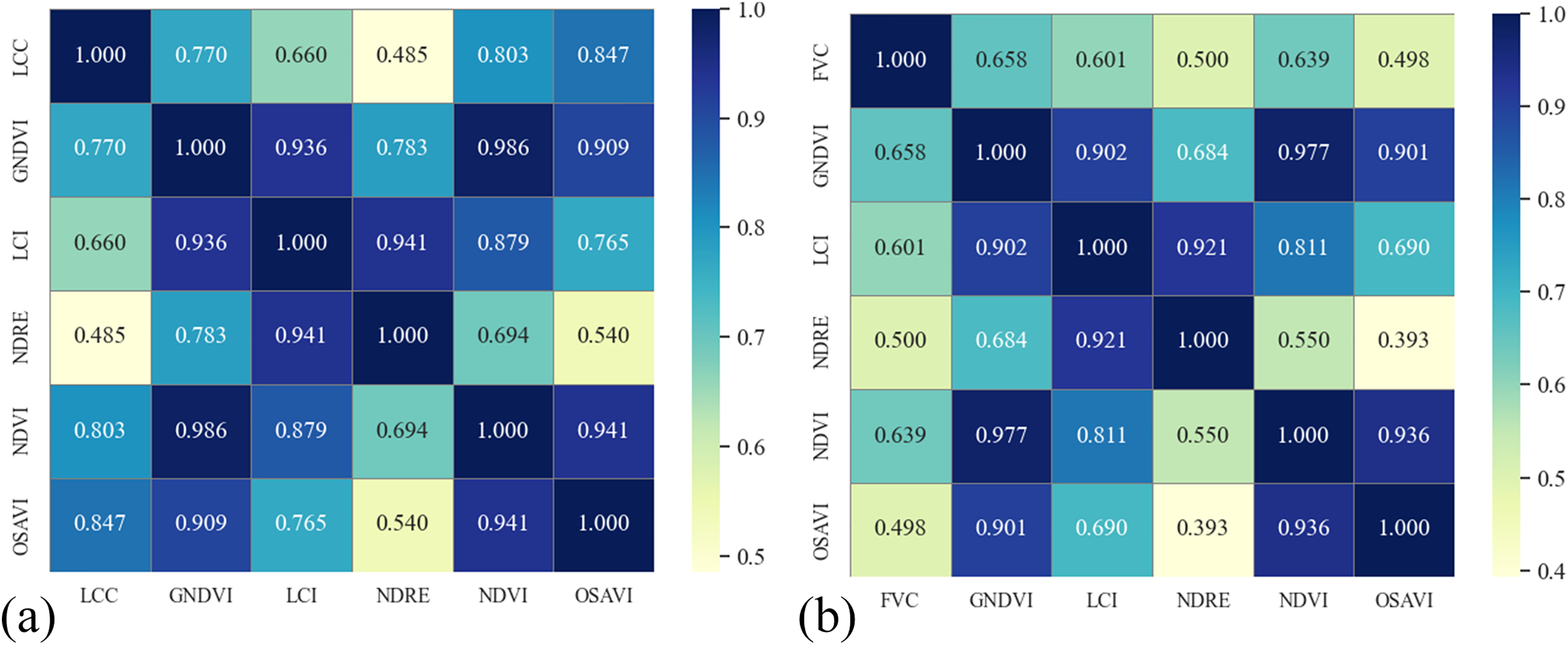
We conducted a correlation analysis using Pearson correlation coefficient to examine the relationship between maize LCC, FVC, and VI obtained from UAV remote sensing, as shown in Fig. 3. The analysis reveals that the correlations between GNDVI, LCI, NDRE, NDVI, OSAVI, and LCC are 0.770, 0.660, 0.485, 0.803, and 0.847, correspondingly. Among them, OSAVI shows the strongest correlation with LCC (0.847), while NDRE exhibits the weakest correlation (0.485). In terms of FVC, the correlations with the five VIs are 0.658, 0.601, 0.500, 0.639, and 0.498, respectively. GNDVI has the strongest correlation with FVC (0.658), while OSAVI has the weakest (0.498). It is worth noting that in this study, the correlation between LCC and NDRE is not as high as that with OSAVI. This may be because the maize growth stage of interest primarily falls within the vegetative growth phase, during which the soil background could affect the relationship between LCC and NDRE. In contrast, OSAVI optimizes soil background, resulting in a higher correlation.
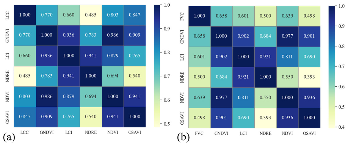
Figure 3: Correlation analysis between vegetation indices and (A) LCC, (B) FVC.
Correlation analysis of texture features with LCC and FVC
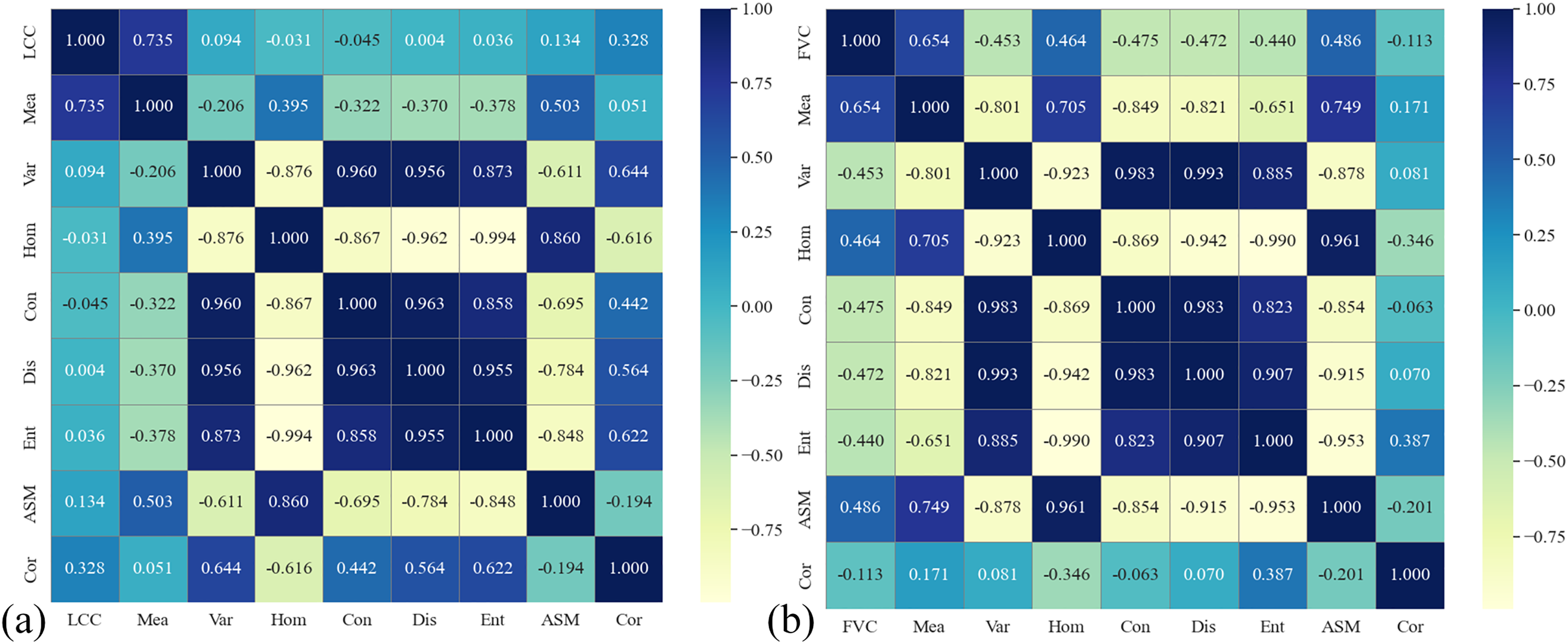
Based on the VI correlation analysis results, the VI images with higher correlations to LCC and FVC were selected. A correlation analysis was then performed between OSAVI image TF and LCC and between GNDVI image TF and FVC. The analysis results are shown in Fig. 4. It can be observed that LCC has a higher correlation with Mea (0.735), while FVC has a higher correlation with Mea (0.654), ASM (0.486), Con (−0.475), and Hom (0.464).
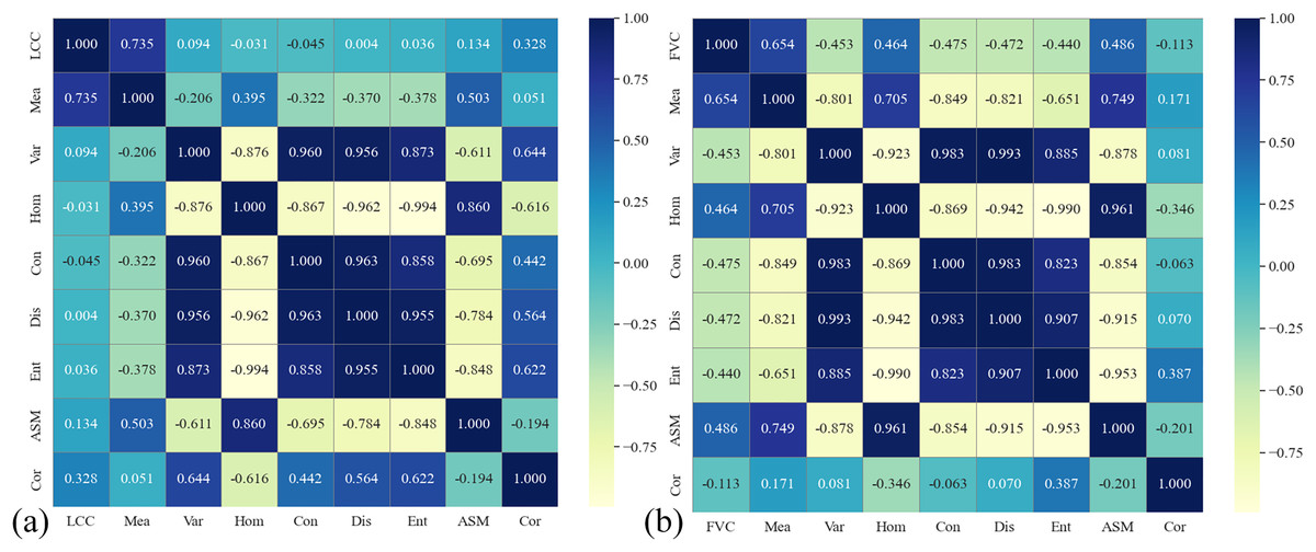
Figure 4: Correlation analysis between texture features and (A) LCC, (B) FVC.
Estimation of LCC and FVC
Estimation of LCC and FVC based on VI
We estimated the FVC and LCC using VI as input. The performance of FVC and LCC estimation under different models is presented in Table 4. It can be observed that when VI is utilized as the input feature in the models, the K-nearest neighbors regression model achieves the best estimation performance for LCC (R2: 0.921, root mean squared error (RMSE): 4.139 Soil-Plant Analysis Development (SPAD) units, mean absolute error (MAE): 3.141 SPAD units), while the GPR model achieves the best estimation performance for FVC (R2: 0.619, RMSE: 0.048, MAE: 0.037).
| Name | Model | R2 | RMSE | MAE | MAPE | Name | Model | R2 | RMSE | MAE | MAPE |
|---|---|---|---|---|---|---|---|---|---|---|---|
| LCC | GPR | 0.910 | 4.434 | 3.517 | 8.695 | FVC | GPR | 0.619 | 0.048 | 0.037 | 4.909 |
| LR | 0.908 | 4.469 | 3.536 | 9.088 | LR | 0.550 | 0.052 | 0.041 | 5.406 | ||
| RR | 0.889 | 4.912 | 4.000 | 9.884 | RR | 0.487 | 0.056 | 0.044 | 5.809 | ||
| RFR | 0.906 | 4.516 | 3.433 | 8.507 | RFR | 0.625 | 0.048 | 0.039 | 5.041 | ||
| SVR | 0.903 | 4.596 | 3.693 | 9.281 | SVR | 0.535 | 0.053 | 0.042 | 5.571 | ||
| KNNR | 0.921 | 4.139 | 3.141 | 8.193 | KNNR | 0.603 | 0.049 | 0.039 | 5.091 |
Estimation of LCC and FVC based on TF
We estimated the FVC and LCC using image TF as input. The estimation performance of FVC and LCC under various models is shown in Table 5. When TF is utilized as the input feature in the models, the KNNR model achieves the best estimation performance for LCC (R2: 0.909, RMSE: 4.771 SPAD units, MAE: 3.631 SPAD units), while the random forest regression model achieves the best estimation performance for FVC (R2: 0.640, RMSE: 0.047, MAE: 0.037).
| Name | Model | R2 | RMSE | MAE | MAPE | Name | Model | R2 | RMSE | MAE | MAPE |
|---|---|---|---|---|---|---|---|---|---|---|---|
| LCC | GPR | 0.884 | 5.379 | 4.324 | 13.596 | FVC | GPR | 0.639 | 0.048 | 0.038 | 4.911 |
| LR | 0.872 | 5.652 | 4.720 | 14.321 | LR | 0.631 | 0.048 | 0.038 | 4.937 | ||
| RR | 0.852 | 6.081 | 5.185 | 16.603 | RR | 0.574 | 0.052 | 0.042 | 5.501 | ||
| RFR | 0.887 | 5.307 | 3.884 | 10.706 | RFR | 0.640 | 0.047 | 0.037 | 4.755 | ||
| SVR | 0.872 | 5.651 | 4.665 | 13.895 | SVR | 0.616 | 0.049 | 0.039 | 5.085 | ||
| KNNR | 0.909 | 4.771 | 3.631 | 10.874 | KNNR | 0.627 | 0.048 | 0.038 | 5.014 |
Estimation of LCC and FVC based on VI + TF
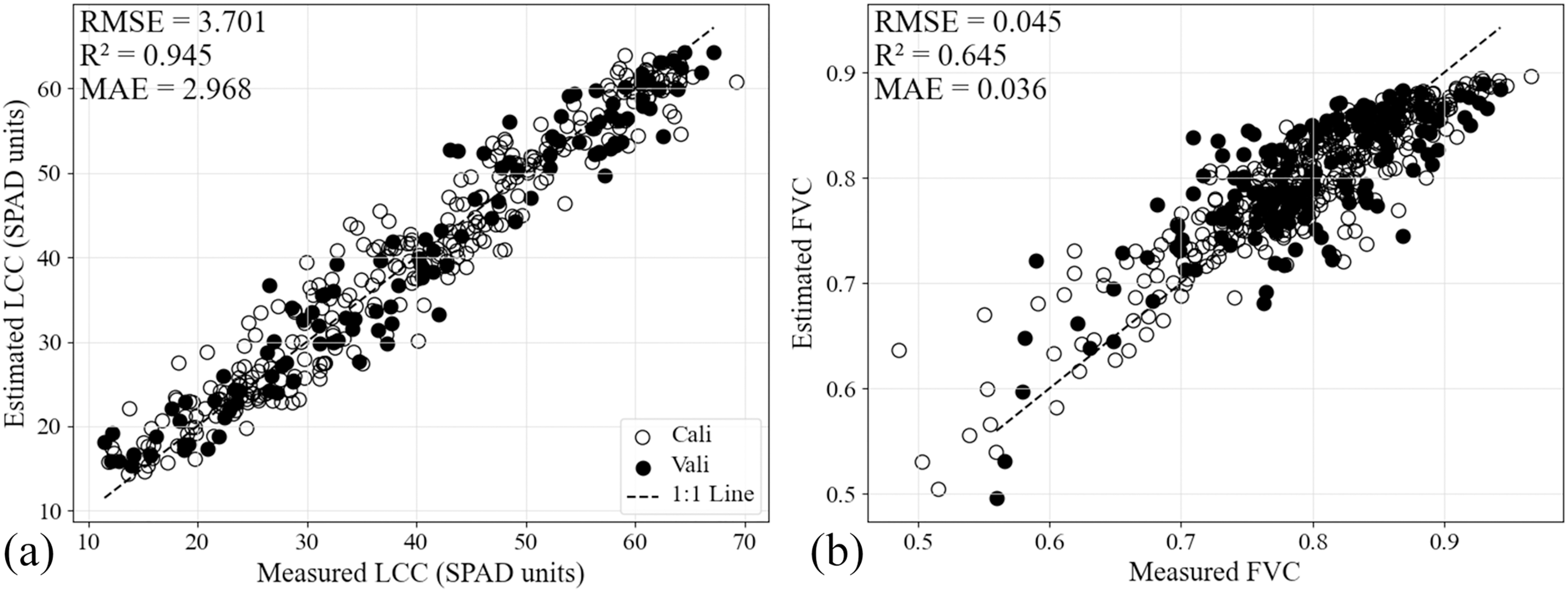
The maize LCC and FVC were estimated by combining UAV remote sensing VI + TF as input variables for different models. As shown in Table 6, when VI and TF are utilized as input feature in the models, the Stacking model demonstrates strongest estimation performance for both LCC (Fig. 5A, R2: 0.945, RMSE: 3.701 SPAD units, MAE: 2.968 SPAD units) and FVC (Fig. 5b, R2: 0.645, RMSE: 0.045, MAE: 0.036). Based on the estimation performance of FVC and LCC under different models (Table 6), this research selects the Stacking regression model with VI + TF used as input feature to estimate LCC and FVC.
| Name | Model | R2 | RMSE | MAE | MAPE | Name | Model | R2 | RMSE | MAE | MAPE |
|---|---|---|---|---|---|---|---|---|---|---|---|
| LCC | GPR | 0.923 | 4.387 | 3.478 | 10.737 | FVC | GPR | 0.577 | 0.049 | 0.039 | 5.057 |
| LR | 0.912 | 4.430 | 3.511 | 10.831 | LR | 0.617 | 0.048 | 0.036 | 4.751 | ||
| RR | 0.894 | 5.135 | 4.275 | 13.524 | RR | 0.579 | 0.049 | 0.039 | 5.113 | ||
| RFR | 0.925 | 4.317 | 3.286 | 9.265 | RFR | 0.635 | 0.047 | 0.037 | 4.693 | ||
| SVR | 0.920 | 4.389 | 3.576 | 10.978 | SVR | 0.560 | 0.050 | 0.040 | 5.116 | ||
| KNNR | 0.923 | 4.386 | 3.549 | 10.449 | KNNR | 0.617 | 0.047 | 0.038 | 4.738 | ||
| Stacking | 0.945 | 3.701 | 2.968 | 9.095 | Stacking | 0.645 | 0.045 | 0.036 | 4.585 | ||
| Bagging | 0.905 | 4.858 | 3.566 | 10.158 | Bagging | 0.603 | 0.047 | 0.037 | 4.839 | ||
| Blending | 0.861 | 5.879 | 4.517 | 12.480 | Blending | 0.379 | 0.059 | 0.047 | 6.130 |
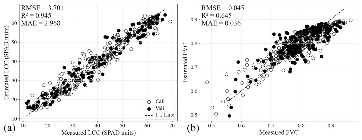
Figure 5: Estimated and measured LCC (A) and FVC (B) from the Stacking ensemble learning.
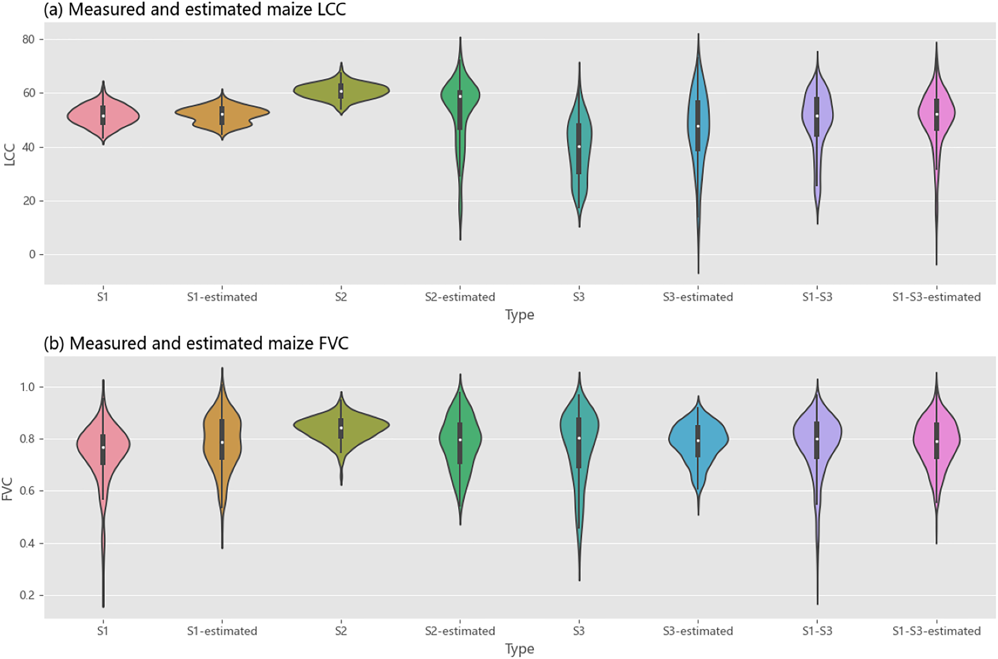
Comparative analyses of the estimated and measured values of LCC (Fig. 6A) and FVC (Fig. 6B) were conducted for S1, S2, S3, and the S1-S3 periods. As shown in Fig. 6A, the estimated values of LCC closely align with the measured values overall. Similarly, Fig. 6B demonstrates that during the S1 to S3 periods, the estimated FVC values were generally consistent with the measured values.
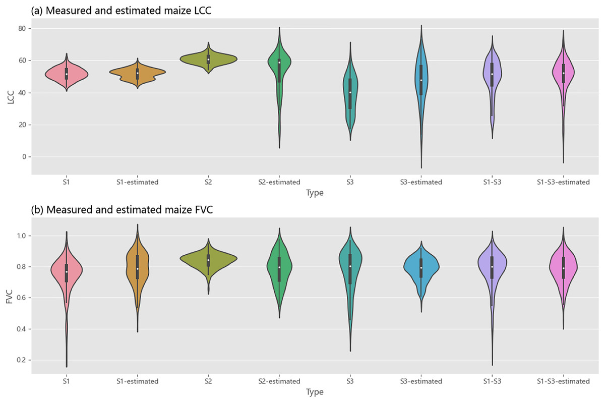
Figure 6: Comparison between estimated and measured LCC (A) and FVC (B).
Mapping of LCC and FVC combining VI and TF
We mapped the LCC and FVC from P1 to P12 stages using the VI + TF as input features and Stacking ensemble learning, as shown in Fig. 7. During the P1 to P4 stages, there is a considerable variation in the LCC of the maize in different planting plots, which is due to phenotypic differences in maize breeding lines. During the P6 to P7 stages, the LCC is generally higher across all plots. At P1, the FVC of all maize planting plots is relatively low, and the differences are minimal. From P2 to P3, some maize breeding lines grow faster, leading to a considerable variation in FVC across planting plots. During the P10 to P12 stages, maize breeding lines are in the reproductive growth stage, and both LCC and FVC gradually begin to decrease. Overall, both LCC and FVC show an upward trend followed by a downward trend, consistent with the field measurement results (Table 1).
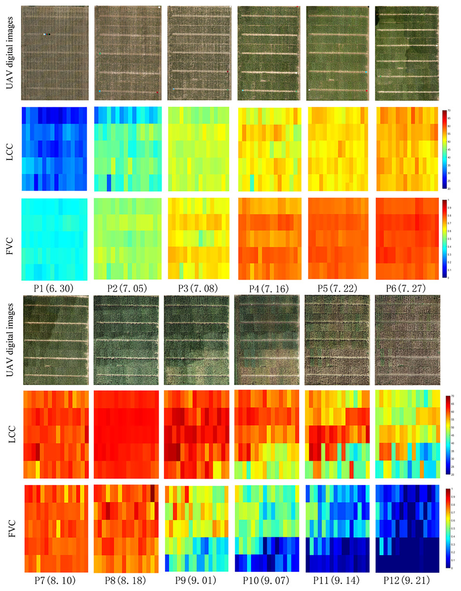
Figure 7: Maize UAV digital images, LCC, and FVC maps.
Note: The color variation in the figure, from blue to red, represents the increase in LCC and FVC from low to high.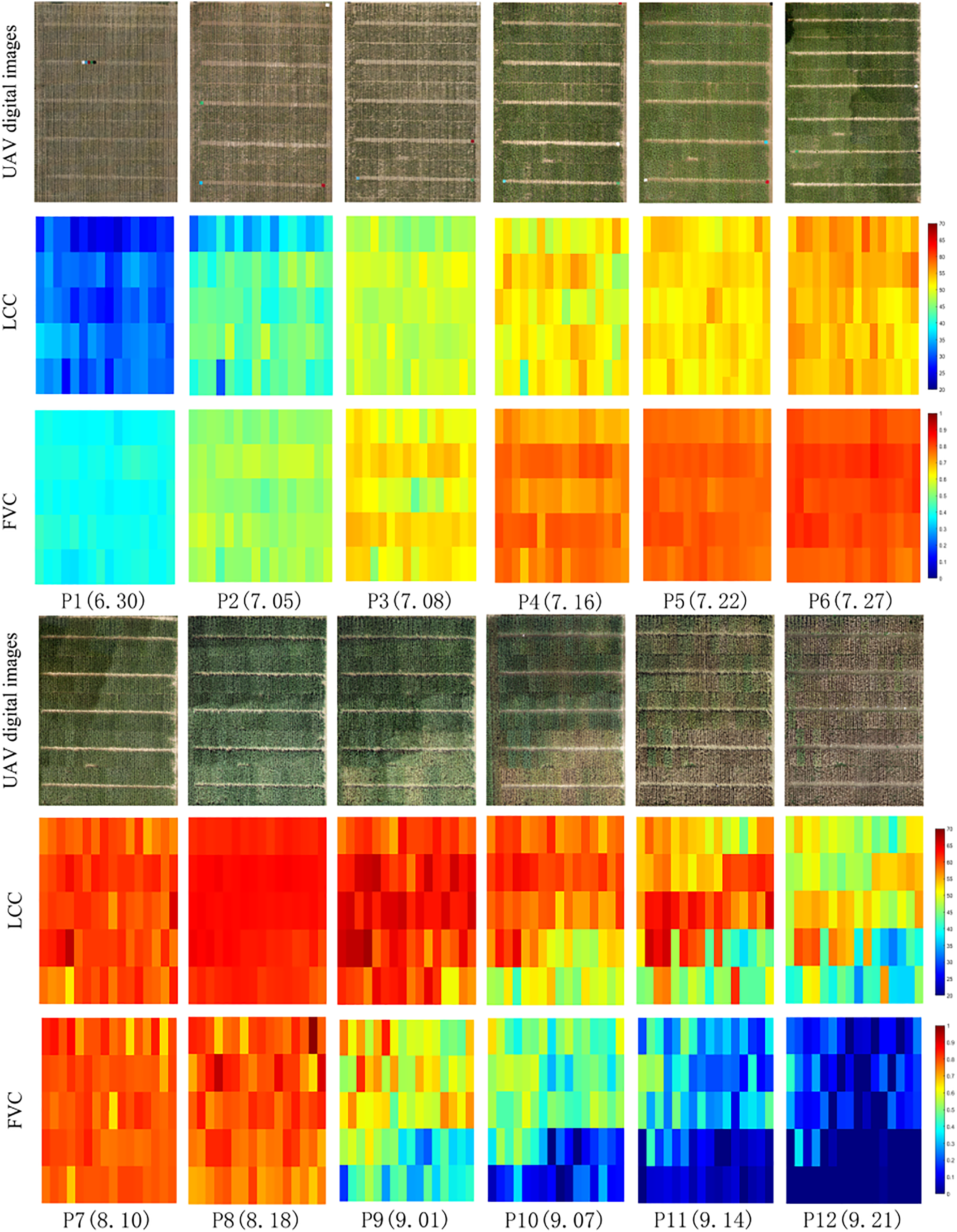
Discussion
The method proposed in this study achieved the optimal estimation accuracy for LCC and FVC due to two primary reasons. First, the integration of spectral features and TF from imagery fully exploited the information contained in remote sensing data. This approach effectively addressed the accuracy limitations caused by the “saturation” phenomenon observed in VI during previous studies. Second, the study utilized an ensemble learning model with superior estimation performance and general applicability. This model demonstrated a strong ability to accurately capture the underlying relationships within the data and to effectively learn from the input features, thereby producing enhanced estimation results.
The relationship between LCC and FVC throughout the growth stages
LCC and FVC are two critical parameters in crop growth research, and they exhibit distinct variation patterns during different growth stages while being interrelated. LCC and FVC are complementary indicators of crop growth. LCC reflects the nutritional status and photosynthetic capacity of the crop, while FVC is closely related to the biomass and canopy coverage. The variation trends of LCC and FVC during different growth stages can provide a more comprehensive understanding of crop growth and physiological processes.
In the early growth stage of the crop, both LCC and FVC are at relatively low levels. During this stage, crops have just begun to germinate or grow, with fewer leaves and relatively low chlorophyll content, leading to a low LCC value. At the same time, due to the smaller leaf area, the FVC value is also low. As the crop progresses into the mid growth stage, leaf expansion accelerates, photosynthesis increases, and the LCC value rises rapidly. Concurrently, the FVC value also increases, as the growth of leaves and stems increases the canopy coverage, forming a denser vegetation layer. In the maturity stage of the crop, the relationship between LCC and FVC changes. Although the number of leaves stabilizes at this stage, LCC may decrease, particularly when the crop enters the physiological senescence phase, where chlorophyll content gradually declines. Meanwhile, FVC may remain at a high level until the crop reaches the final harvesting stage, at which point some leaves may wilt, and the FVC may decrease.
The impact of VI and TF on crop parameter estimation
Based on spectral and TF combined with ensemble learning models, a study was conducted on the estimation of maize LCC and FVC. As shown in Table 6, when VI and TF were combined as input features for the model, the Stacking model achieved the best estimation performance for LCC (R2: 0.945, RMSE: 3.701 SPAD units, MAE: 2.968 SPAD units) and FVC (R2: 0.645, RMSE: 0.045, MAE: 0.036). A comparative analysis of the two input scenarios (VI and TF): when VI is used as input, the estimation of LCC is superior to when TF is used as input. This is because VI, as an indicator that represents the vegetation status on the surface, is more sensitive to changes in vegetation color, making it better suited for estimating LCC. Conversely, when TF is used as input, the estimation of FVC is better than when VI is used. This is because FVC reflects the structure and spatial distribution of crops, and TF is more sensitive to fine structural changes on the surface of vegetation, which makes it more effective for estimating FVC.
UAV remote sensing technology provides high spatiotemporal resolution multi-spectral imagery, which is essential for rapid and detailed monitoring of crop stress, growth conditions, and other agricultural parameters. Compared to traditional remote sensing methods, small agricultural UAV can easily adjust the timing and frequency of data collection, making them adaptable to research needs across different temporal and spatial scales. The VI obtained from the sensors onboard these UAV can be used to diagnose crop growth status on the surface. However, factors like soil background can affect the VI, making it difficult for spectral VI alone to fully capture the dynamic changes in crop FVC and LCC. Additionally, during the mid and late growth stages of crops, where canopy coverage is high, VI may saturate, losing sensitivity to LCC and FVC changes. This study attempts to combine spectral VI with crop canopy TF to improve the accuracy of FVC and LCC estimation. Image TF, which describe the surface properties of objects in the image or region, are highly sensitive to crop canopy structures. Combining VI and TF helps further enhance the ability of remote sensing technologies to capture changes in LCC and FVC, leading to more accurate estimates.
In this study, the low quality of LAI data may have affected the estimation accuracy of FVC. LAI is a key indicator reflecting the leaf area of crops and is commonly used to estimate biomass and coverage. LAI data can be influenced by factors such as sensor errors, variations in environmental conditions, and soil background, which lead to inaccuracies in estimation and, consequently, affect the FVC prediction. When the quality of LAI data is insufficient, it is difficult to accurately reflect the crop growth status, which in turn impacts the FVC values derived from LAI. Future research will focus on improving the quality of LAI data. In addition, FVC changes are also influenced by factors such as soil type, climate conditions, and crop management, which exhibit considerable variability in remote sensing data, increasing the complexity of FVC prediction. Although ensemble learning models have effectively improved prediction accuracy, challenges remain in addressing these diverse factors.
The sensitivity of specific spectral regions—particularly the RE, R, and NIR bands—played a critical role in capturing maize phenological dynamics. As demonstrated in our analysis, OSAVI and NDRE exhibited strong correlations with LCC. This aligns with known biophysical principles: the R band corresponds to chlorophyll absorption minima, the RE band is highly sensitive to subtle changes in chlorophyll concentration and leaf internal structure, while the NIR band responds to canopy structural properties like leaf area and density.
Notably, emerging research (Bartold & Kluczek, 2023) suggests chlorophyll fluorescence (ChF), especially solar-induced fluorescence (SIF) in the red and far-red spectrum, may provide an even more direct and sensitive indicator of photosynthetic activity and phenological transitions than LCC alone. Future work with UAVs equipped with hyperspectral or specialized fluorescence sensors could bridge this gap, enabling combined LCC-ChF monitoring for enhanced phenological tracking.
While our correlation analysis provided initial insights into feature-target relationships, the study by Bartold & Kluczek (2024) which utilized gain parameters, and research employing Mean Decrease Accuracy (MDA) (Bartold et al., 2024), rightly emphasize the broader scientific value of formal feature importance assessment within machine learning frameworks. Future studies should consider incorporating these metrics to strengthen the experimental design.
The advantages of ensemble learning estimation models
Machine learning, while powerful, relies heavily on large training datasets and complex hyperparameter tuning. Its training process typically requires substantial computational resources and time (Yang & Shami, 2020). The generalization performance of single machine learning models is closely related to the volume of data and the regularization techniques employed. Despite their strong learning capabilities, single-machine learning model can suffer from overfitting or underfitting when training data is limited or has substantial distribution shifts (Lou, Lu & Li, 2024). Compared to single machine learning models, Stacking models have lower computational complexity. The individual base learners can be trained in parallel and then combined for prediction, which makes the model more computationally efficient.
Ensemble learning generally offers good generalization capabilities. Since ensemble learning models combine the strengths of multiple individual models, they often maintain high performance across different datasets and application scenarios, reducing the risk of overfitting. Ensemble learning can also integrate various types of models, including linear and nonlinear models, making it more adaptable and flexible when handling complex problems. With its ability to improve accuracy, robustness, generalization ability, and the flexibility of model integration, ensemble learning has become an indispensable method in modern machine learning. Stacking models are particularly advantageous when resources are limited or quick model iteration is needed, making them a viable option for real-time monitoring or decision support systems in agricultural applications. By selecting the Stacking ensemble learning model, which has strong generalization capabilities, and combining VI and TF as input features, the advantages of VI and TF in different aspects of crop parameter estimation can be fully utilized, resulting in more accurate estimation outcomes.
The importance of ensemble learning models in this study is reflected in several aspects. First, by combining multiple base learners, ensemble learning mitigates the overfitting issues associated with single models, thereby enhancing prediction stability. Second, ensemble learning demonstrates greater robustness to noise and outliers, effectively improving the reliability of the results. Lastly, ensemble learning can flexibly adapt to complex agricultural data, enhancing the computational efficiency and generalization ability of the model, making it particularly suitable for real-time monitoring and rapid model iteration applications.
Although the ensemble model achieved the highest FVC estimation accuracy (R² = 0.645), this value remains modest, suggesting room for improvement. Future studies should explore incorporating structural features (e.g., canopy height distribution from LiDAR) or auxiliary data (e.g., meteorological variables) to potentially enhance prediction performance.
Limitations of UAV remote sensing
UAV data present limitations, such as sensitivity to soil background reflectance during early growth stages, relatively limited spectral resolution (often lacking continuous coverage in key regions like the red-edge) compared to dedicated airborne or satellite hyperspectral sensors, and practical constraints on area coverage compared to satellite data like Copernicus Sentinel-2. As demonstrated by Gurdak & Bartold (2021) vegetation indices derived from Copernicus satellite data for maize and sugar beet effectively tracked changes associated with plant aging, such as the SIPI index. Despite these limitations, UAVs excel at high-frequency, detailed field-scale monitoring, which is crucial for precision breeding and management applications.
Finally, we explicitly acknowledge a key limitation inherent to UAV-based optical monitoring: significant sensitivity to soil background noise, particularly during early growth stages when crop canopy coverage is sparse. Soil reflectance variations can substantially confound spectral signals from vegetation, impacting VI accuracy for both LCC and FVC estimations. While the soil-adjusted OSAVI employed in this study partially mitigates this issue, more robust solutions are needed (Dąbrowska-Zielińska et al., 2012).
SAR systems are uniquely advantageous due to their all-weather operational capability and sensitivity to soil properties like moisture content and surface roughness. Integrating SAR-derived soil moisture and roughness parameters with UAV-acquired spectral and textural features offers a multi-sensor approach to decouple the influence of soil background from crop canopy signals. This synergistic data fusion holds significant potential for not only minimizing early-stage estimation errors caused by soil noise but also enabling the retrieval of complementary biophysical parameters relevant to maize growth assessment. Future investigations will explore this integrated UAV-SAR framework.
A critical limitation of UAV optical remote sensing is its susceptibility to soil background noise, particularly during early growth stages when vegetation cover is sparse. SAR systems uniquely penetrate cloud cover and are insensitive to solar illumination conditions. Crucially, SAR backscatter coefficients directly respond to soil biophysical properties—including surface roughness and moisture content—which are key parameters influencing crop growth but inaccessible to optical sensors Soil spectral variations can significantly interfere with vegetation signals, reducing the accuracy of VI-based estimations for both LCC and FVC.
Conclusions
This study integrates spectral and TF from UAV imagery as input variables to evaluate the feasibility of three ensemble learning models: Stacking, Bagging, and Blending for high-precision maize LCC and FVC estimation. The study leads to the following conclusions:
-
(1)
Spectral features and TF represent complementary aspects of maize crop growth information derived from remote sensing imagery. Spectral features effectively capture changes in LCC driven by the light absorption by maize leaves, while TFs are better suited to reflect variations in the maize canopy structure. Combining these features enhances the sensitivity of detecting changes in maize LCC and FVC.
-
(2)
The Stacking ensemble learning model outperforms traditional individual machine learning models for estimating LCC and FVC. By overcoming the limitations of individual models, the Stacking approach mitigates overfitting and enhances the stability of crop parameter estimation models. In this study, when spectral and TFs were jointly used as input variables, the Stacking ensemble learning model achieved optimal estimation performance for LCC (R2: 0.945, RMSE: 3.701 SPAD units, MAE: 2.968 SPAD units) and FVC (R2: 0.645, RMSE: 0.045, MAE: 0.036).
-
(3)
The optimization of the Stacking ensemble learning model typically requires iterative adjustments to its hierarchical structure, making it challenging to quantify the specific contributions of each base learner to the prediction results. Future research should focus on applying optimization algorithms and hyperparameter tuning techniques to simplify the complexity of Stacking models. Such advancements will enhance the model’s practicality and promote its application in agricultural remote sensing data analysis.