
Corn grain year identification based on Raman spectroscopy and machine learning
- Published
- Accepted
- Received
- Academic Editor
- Consolato Sergi
- Subject Areas
- Artificial Intelligence, Computer Vision, Data Mining and Machine Learning
- Keywords
- Raman spectroscopy, Machine learning, Pretreatment, Feature extraction, Support vector machine
- Copyright
- © 2025 Miao et al.
- Licence
- This is an open access article distributed under the terms of the Creative Commons Attribution License, which permits unrestricted use, distribution, reproduction and adaptation in any medium and for any purpose provided that it is properly attributed. For attribution, the original author(s), title, publication source (PeerJ Computer Science) and either DOI or URL of the article must be cited.
- Cite this article
- 2025. Corn grain year identification based on Raman spectroscopy and machine learning. PeerJ Computer Science 11:e3355 https://doi.org/10.7717/peerj-cs.3355
Abstract
Background
As one of the important food crops, corn’s reserve issue has attracted much attention. Given the direct impact of corn year on its quality and supply, as well as the limitations of traditional manual identification methods, this study aims to explore the feasibility of combining Raman spectroscopy with machine learning methods in corn year identification.
Methods
Five different years of corn were selected as experimental samples, and spectral data of corn were obtained through Raman spectroscopy. The spectral data were subjected to a combination of preprocessing methods such as convolution smoothing (SG), wavelet transform (WT), standard normal variable transform (SNV), and first derivative processing. Then, important feature information is extracted through dimensionality reduction using linear discriminant analysis (LDA) and independent component analysis (ICA). Finally, year recognition is achieved through support vector machine (SVM), random forest, and K-nearest neighbor algorithm.
Results
The experimental results show that the proposed method exhibits good year recognition performance. Among them, the combination of SG and SNV preprocessing and ICA feature extraction significantly shortened the running time and improved the recognition accuracy. The SVM classification model performs the best, with an accuracy of up to 96.69%, a recall rate and F1 value of 96.77% and 0.9659, respectively, and a running time of only 99.53 s, indicating that the model based on Raman spectroscopy and machine learning can efficiently and accurately identify corn years.
Introduction
Corn is the first grain crop in China, and it is also a valuable resource with a wide range of applications. It meets people’s demand for food rations and serves many fields such as industrial consumption and livestock feed. With its diverse and developable products, corn deep processed products have penetrated into multiple industries such as food, medicine, and materials, making the assurance of their quality and safety crucial (Fu, 2024). For grain processing enterprises, reserved grain also plays an indispensable role. Amid market price fluctuations, these enterprises may struggle to procure sufficient grain directly from the market; thus, they rely on corn reserves from national stockpiles to sustain their production operations. China has achieved basic self-sufficiency in food supply, and the government attaches great importance to this by expanding grain reserve capacity. This measure has exerted a positive effect on meeting consumers’ food demand. Currently, China’s grain reserves are sufficient to cover approximately 5–10 years of consumption. The reason why the reserve can be maintained for such a long time is largely due to the advanced grain preservation technology in China (Sinograin, 2015), which enables the reserve grain to maintain excellent condition for a long time, and even makes it difficult to accurately determine its storage year based solely on appearance. Given this, there is an urgent need for a fast, efficient, and cost-effective detection method to accurately identify the storage year information of corn.
There is relatively little research on the year identification of corn both domestically and internationally, mainly focusing on the identification of different types of corn seeds RNN (Yang & Hu, 2023; Si et al., 2023; Li et al., 2024a), seed vitality detection (Yang et al., 2022; Wang et al., 2022; Wang & Song, 2024), and disease identification (Xu et al., 2023; Zhang & Huang, 2024). Ali et al. (2020) obtained mixed feature data from corn seed images and classified them using hybrid features. Pang et al. (2020) achieved good results in detecting seed vitality by modeling the collected hyperspectral image data and classifying the raw data after processing. Wang et al. (2021) established a model using spectral data with different band widths, and selected effective variables through competitive adaptive reweighted sampling. While ensuring the accuracy of maize seed vigor discrimination, the overall computational complexity was effectively reduced, indicating the importance of feature extraction. Meng et al. (2022) used near-infrared spectroscopy technology to study corn seed ear rot disease and identified it by extracting characteristic information. Yang et al. (2023) used hyperspectral technology combined with relevant algorithms to extract characteristic wavelengths for identifying the purity of corn seed varieties. Wu et al. (2022) proposed combining hyperspectral technology with ensemble learning for corn seed moisture detection. The prediction accuracy and stability were high in the training set, but the effect on the test set was average. Xia et al. (2024) combined hyperspectral data with physicochemical parameters and used machine learning to identify seeds, resulting in average accuracy. The rapid development of artificial intelligence technology is accompanied by various detection and classification techniques (Zhang et al., 2022; Ma et al., 2023) being used in research related to grain crops such as rice and corn.
Machine learning is an artificial intelligence technology that automatically discovers patterns and features in data through algorithms, enabling classification and prediction of new data (Dhar et al., 2021). Wang (2022) explored the recognition of corn seed varieties through image recognition technology. The collected corn seed images contain category information, and by establishing a model for classification and recognition, a 92% accuracy rate can be obtained. Fan et al. (2022) improved the existing You Only Look Once (YOLO) v4 model by optimizing the internal network structure to enhance its performance. The final improved model was used for the appearance quality detection of corn seeds, which improved the model recognition rate and enhanced its robustness. Due to the input being image data, the experimental process may be time-consuming. Ma et al. (2022) added attention mechanisms to the model to identify corn seed category information and improved the network to reduce model training time. However, due to the input of multiple image data and the large number of network model parameters, the overall training time is relatively long. Li et al. (2024b) used deep learning methods to identify hyperspectral images of corn seeds, enhanced the classification performance of the model through dimensionality reduction methods, and reduced redundant features, effectively reducing the training time of the model. In recent years, thanks to the outstanding ability of machine learning in feature learning, Raman spectroscopy has developed into an alternative method seeking to improve the performance of classification problems.
Raman spectroscopy, as an efficient detection technology, has shown great potential in quickly identifying corn varieties, origins, and years due to its fast and non-destructive characteristics (Cialla-may, Schmitt & Popp, 2019). It plays a crucial role in maintaining the safety and stability of the grain market. This article proposes a method for identifying corn years based on Raman spectroscopy combined with machine learning models. Spectral data of corn germ from five different years are extracted, and the spectral data is processed using convolution smoothing and wavelet transform combined with standard normal variable transformation and first-order derivative preprocessing methods. Then, feature extraction is achieved through dimensionality reduction methods independent component analysis (ICA) and linear discriminant analysis (LDA) to obtain feature vectors containing important information. Finally, support vector machine (SVM), random forest (RF), and K-nearest neighbor (KNN) algorithms are used for training and classification. After multiple experiments, a highly accurate recognition model was obtained, providing reference for further research in the future.
Materials and Methods
Materials
Corn as an important grain crop in Northeast China, has been stored for a long time. The experimental samples were sourced from the market. The variety is Jidan 27 and the number of samples is 277, and different years of corn were selected and numbered, namely 2014, 2015, 2018, 2019, and 2020, as shown in Fig. 1.
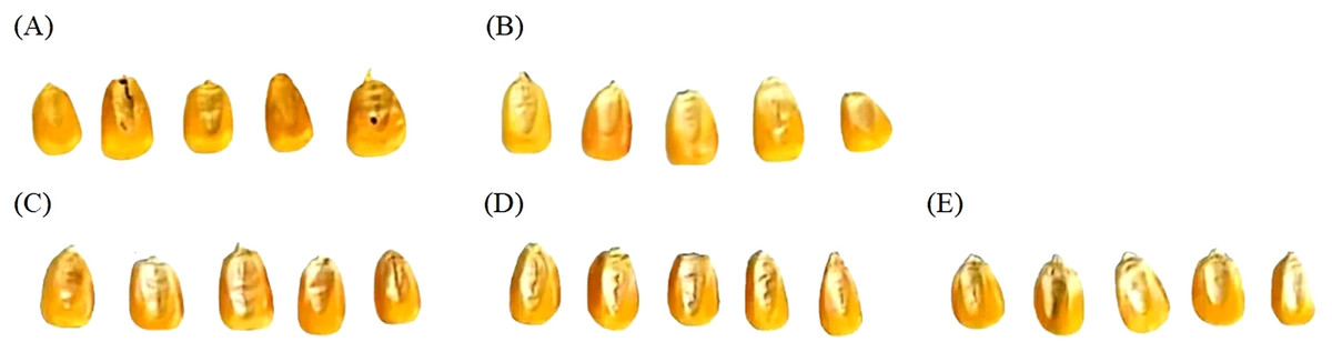
Figure 1: Corn sample images from different years.
(A) 2014. (B) 2015. (C) 2018. (D) 2019. (E) 2020.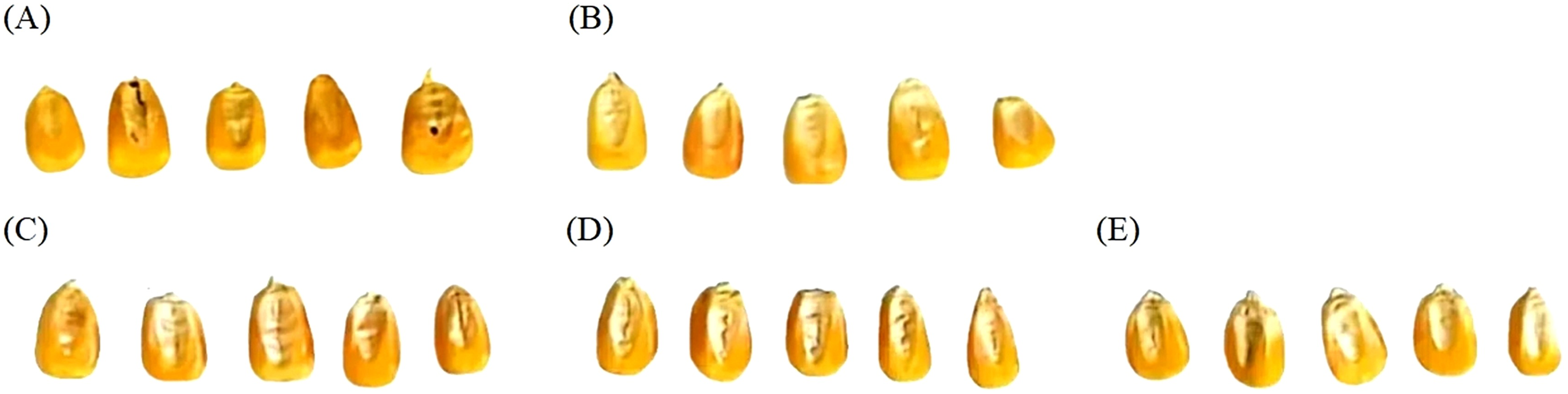
Instruments and data collection
The TriVistaTMM555CRS micro area three-level Raman spectrometer produced by Princeton company was selected for the experiment. The instrument adopts liquid nitrogen refrigeration technology and the temperature is as low as −120 °C. The excitation light source is the MW-GL semiconductor laser produced by Changchun Laishi Optoelectronics Technology Co Ltd. with a wavelength of 532 nm, a linewidth of 0.1 nm, and a power range of 0–500 mW. During the detection process, the laser energy is controlled within 2 mW to avoid damaging the internal structure of the object. The excitation wavelength of the light source is 532 nm, the effective area of the grating of the Raman spectrometer is 68 × 84 mm, and the spectral resolution is 0.6 cm−1.
During the experiment, the selected corn kernels were placed on a glass slide, and a Raman spectrometer was used to measure the corn germ and collect Raman signals. In order to avoid photolysis caused by long-term light exposure, each sample was scanned five times, and in order to reduce the deviation of measurement results, multiple measurement results were averaged. Finally, the whole data set consisted of 277 spectral data. Figure 2 shows the process of Raman spectroscopy acquisition. The laser light source emits laser light through the Raman detection probe and irradiates it onto the experimental sample. Then, the collected information is processed by the Raman spectrometer and returned to the upper computer.
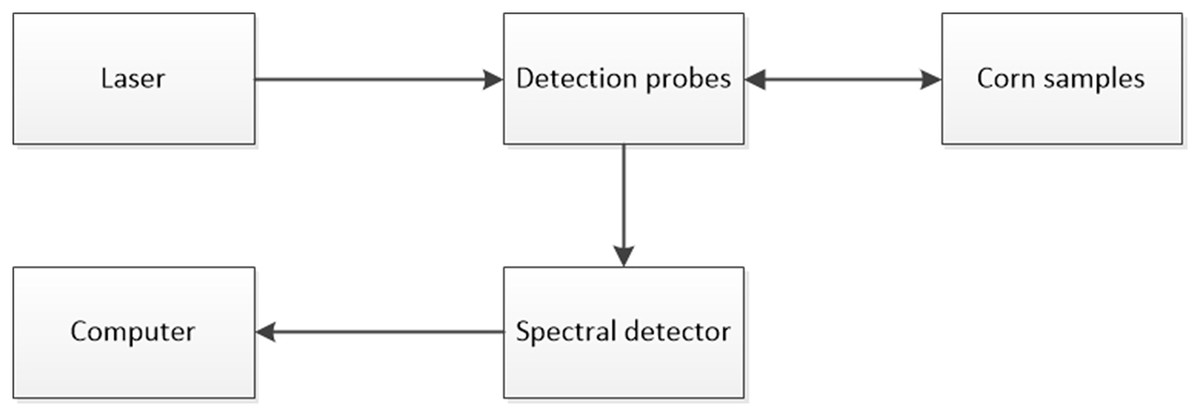
Figure 2: Raman spectroscopy acquisition process diagram.
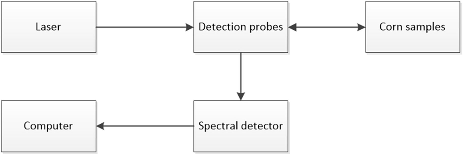
Spectral data preprocessing
To enhance the intensity of the original Raman spectral signal, highlight the Raman peaks, and determine their positions and intensities, preprocessing methods combining convolutional smoothing (Savitzky Golay, SG) and wavelet transform (WT) with standard normal variable transformation (SNV) and first derivative were employed. These preprocessing steps aim to optimize spectral data to better reflect feature information, thereby facilitating subsequent feature extraction and the application of machine learning algorithms in year recognition.
Convolutional smoothing and wavelet transform can effectively eliminate noise, suppress or remove random errors superimposed on the original spectral signal. SNV (Zhang et al., 2024) is a commonly used preprocessing method, mainly used to reduce the influence of other factors such as solid particles on spectra. SNV can also correct spectral errors through the standard normal method. The spectral data processed by SNV can be obtained through Eq. (1).
(1)
Among them, represents variance, represents the mean.
The first derivative can eliminate the fixed deviation between the absorbance at a certain wavelength in the spectrum and the true value, and identify and eliminate outliers (Xiang et al., 2023). Due to the potential increase in noise caused by using first-order derivatives, it is generally better to use SG or WT for denoising before taking the derivative. The selection of window size during smoothing is also very important, and appropriate smoothing processing can preserve more detailed information.
Model establishment and evaluation
In predicting sample production year information, constructing an accurate classification model is an indispensable and critical step. Prior to model establishment, feature extraction must be performed on the preprocessed spectral data, the process aimed at converting complex spectral information into analyzable feature vectors. However, excessively high feature dimensionality can significantly increase computational complexity and may negatively impact classification accuracy. To ensure optimal classification performance, the sample size of the data matrix should be substantially larger than the number of features; this is an effective strategy to prevent overfitting and enhance the model’s generalization ability. Following data preprocessing, dimensionality reduction must be implemented promptly to extract the most representative features from the data. This step is critical for improving model efficiency and accuracy, thereby laying a solid foundation for subsequent accurate prediction of production year information.
Independent component analysis (ICA) is a machine learning algorithm used to decompose multivariate complex signals (Miettinen et al., 2020). The received source signal is affected by noise and independent signals from other sources, making it difficult to record clean measurement values. The measurement results can be understood as a summary of several independent signals, and blind source separation can be used to separate these mixed signals.
ICA can separate mixed signals into multiple independent signals, with the ultimate goal of finding a set of signals that can represent the overall information and are as independent as possible between them. The entire process is a dimensionality reduction operation that extracts effective features while also reducing overall complexity.
The goal of ICA is to separate each component from a linear superposition of several independent components, and its steps can be summarized as follows:
-
(1)
Subtract the mean of the data and shift it to the origin as the center
-
(2)
Transform the covariance matrix of data into a unit matrix through rotation and scaling (whitening process)
-
(3)
Minimize mutual information between various components of data through rotation (approximately independent)
LDA is a supervised analysis algorithm that uses feature information and real categories to model and predict the categories to which other data belong (Xie et al., 2020). LDA aims to make data with the same label more compact and data with different labels more dispersed through dimensionality reduction. This process relies on matrix factorization to achieve dimensionality reduction of data, and the dimensionality of the reduced data will be less than the number of categories. The dimensionality reduction steps of LDA can be summarized in the following steps:
-
(1)
Obtain the intra class divergence matrix and inter class divergence matrix through the global mean and sample mean of the dataset
-
(2)
Calculate the maximum d eigenvalues of matrix
-
(3)
Calculate the eigenvectors corresponding to d eigenvalues and use them as the dimensionality reduction matrix W
-
(4)
Multiply the original dataset with the dimensionality reduction matrix to obtain a d-dimensional dataset for dimensionality reduction operation
Based on the extracted feature information, machine learning algorithms can be used for training and classification. During the experiment, three classification models were selected: support vector machine, random forest, and K-nearest neighbor algorithm.
SVM as a classic machine learning algorithm, is applied in various classification tasks and can achieve good results in binary or multi classification tasks. It uses a nonlinear mapping relationship to map data into high-dimensional space, forming a hyperplane to partition the data, and optimizing to find the optimal hyperplane.
RF is an ensemble learning method that combines the prediction results of multiple decision trees to improve the accuracy and stability of the model. Random forest constructs multiple decision trees and combines their prediction results to obtain the final prediction result. These decision trees are independently generated during the training process, with each tree trained using randomly selected samples and features from the original dataset. The final prediction result is obtained by voting on the prediction results of all trees.
KNN algorithm is a commonly used method for classification. In KNN, the classification result of an object is determined by the voting or average of its nearest K neighbors. If most of the K most similar samples in the feature space belong to a certain category, then the sample also belongs to that category.
Spectral data preprocessing, feature extraction, and model establishment were all run on PyCharm 2023. During the experiment, all sample data were partitioned using relevant algorithms, and each group was tested multiple times. Various evaluation metrics were averaged to represent overall performance, including accuracy, recall, F1 score, and running time.
Results
Preparation and analysis of raman spectroscopy
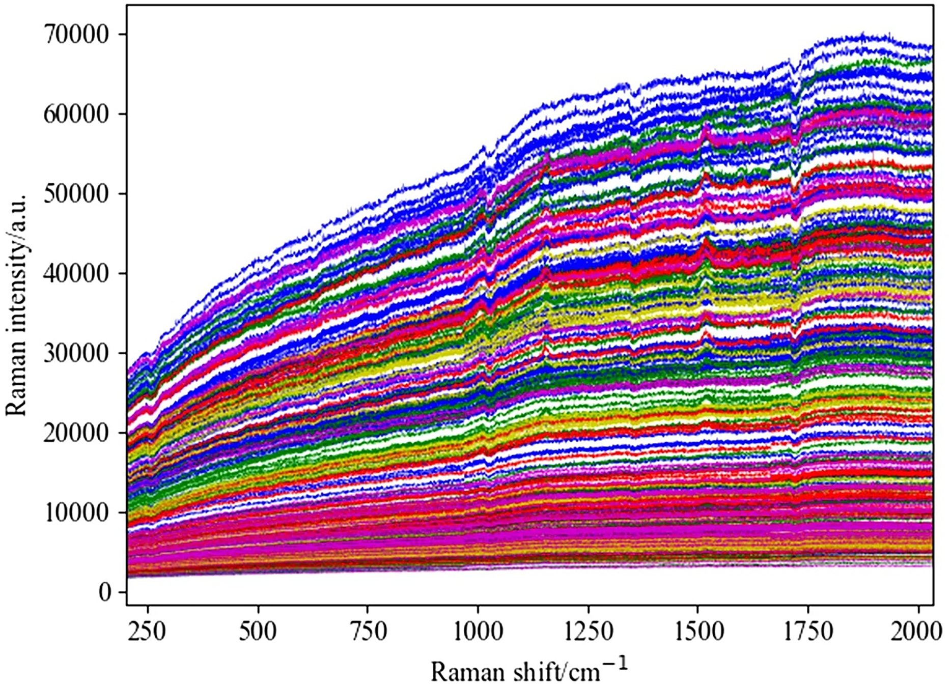
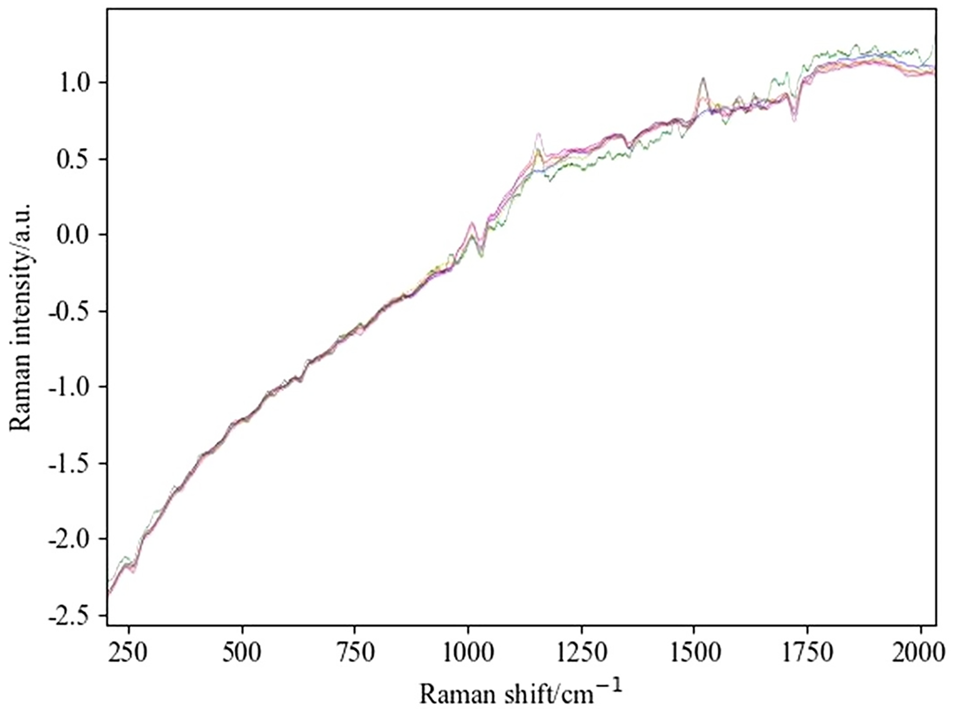
This study retained spectral data in the range of 202–2033 cm−1 as the initial input spectral data for the experiment. Figure 3 shows the original Raman spectrum, which distinguishes data from different years with different colored lines. Figure 4 shows the spectrogram after convolution smoothing combined with SNV and first-order derivative processing, while Fig. 5 shows the spectrogram after wavelet transform combined with SNV and first-order derivative processing. Figure 6 shows the spectrum difference diagram of maize in different years. From the diagram, it can be seen that the intensity of characteristic peaks in the spectrum diagram of maize in different years is different, and there are obvious characteristic peaks near 1,000 cm−1, 1,150 cm−1 and 1,530 cm−1.
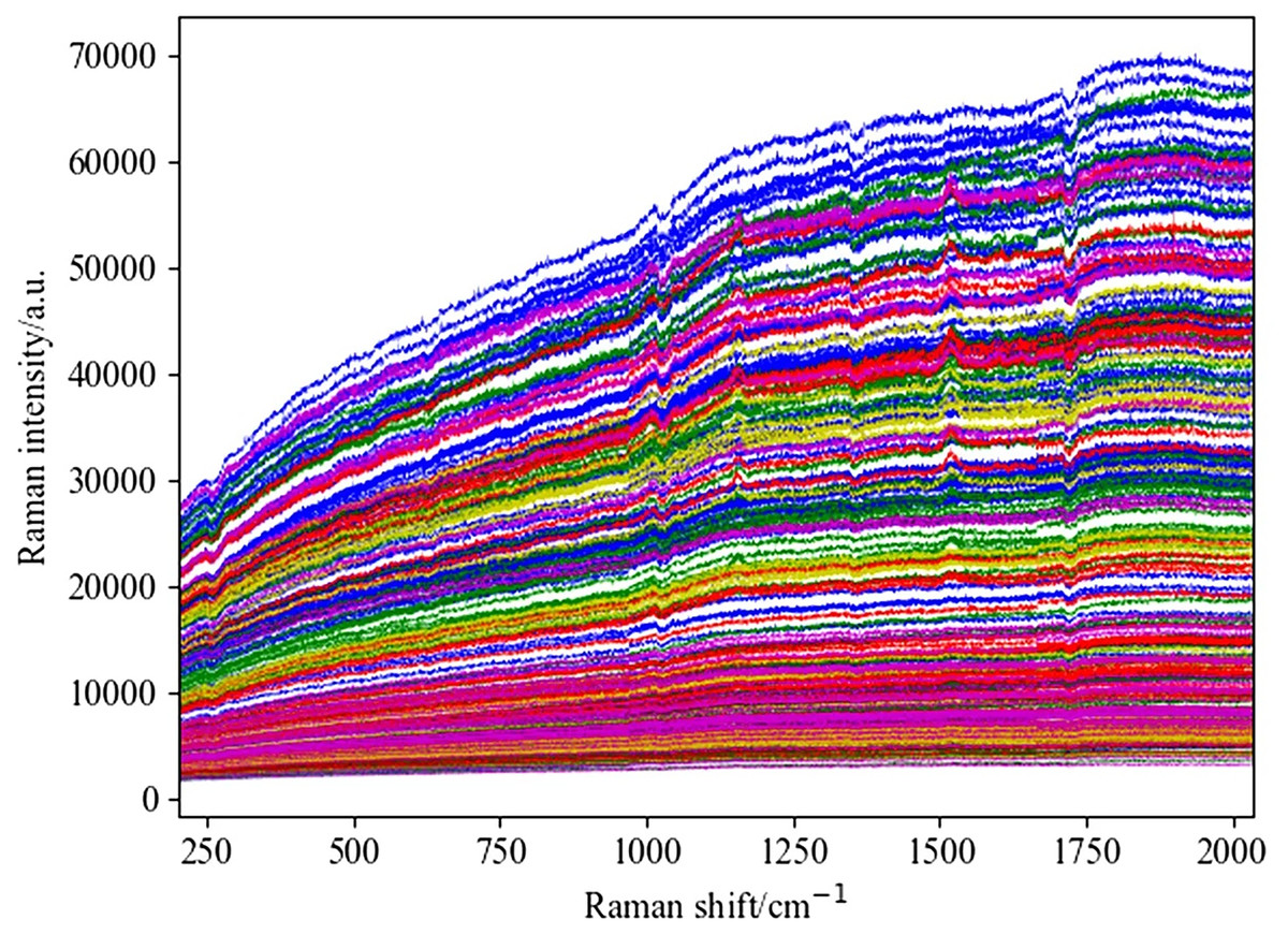
Figure 3: Original spectra of corn stored in five different years.
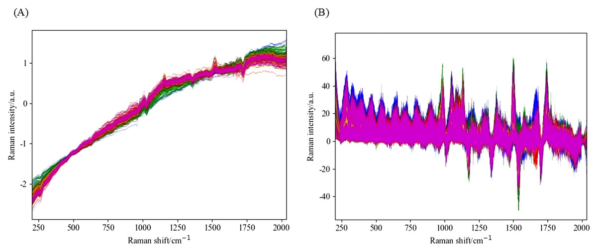
Figure 4: Spectral diagram of SG combined with SNV and first-order derivative processing.
(A) The spectrum of SG and SNV combined processing. (B) The spectrum obtained by combining SG and first derivative processing.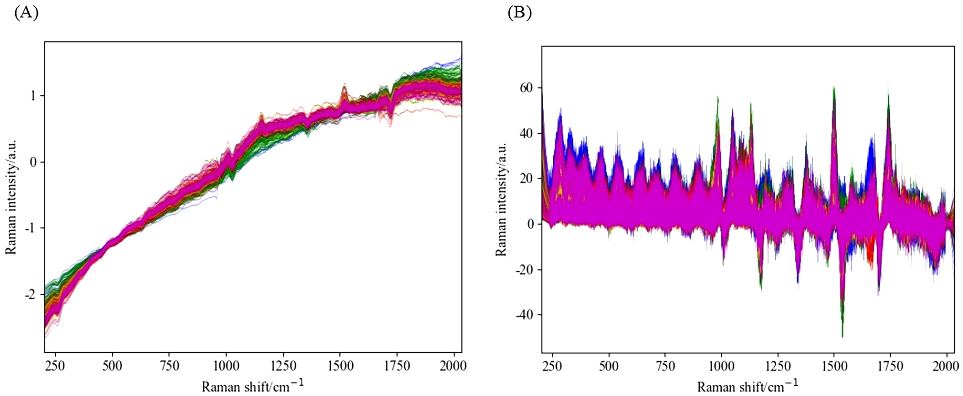
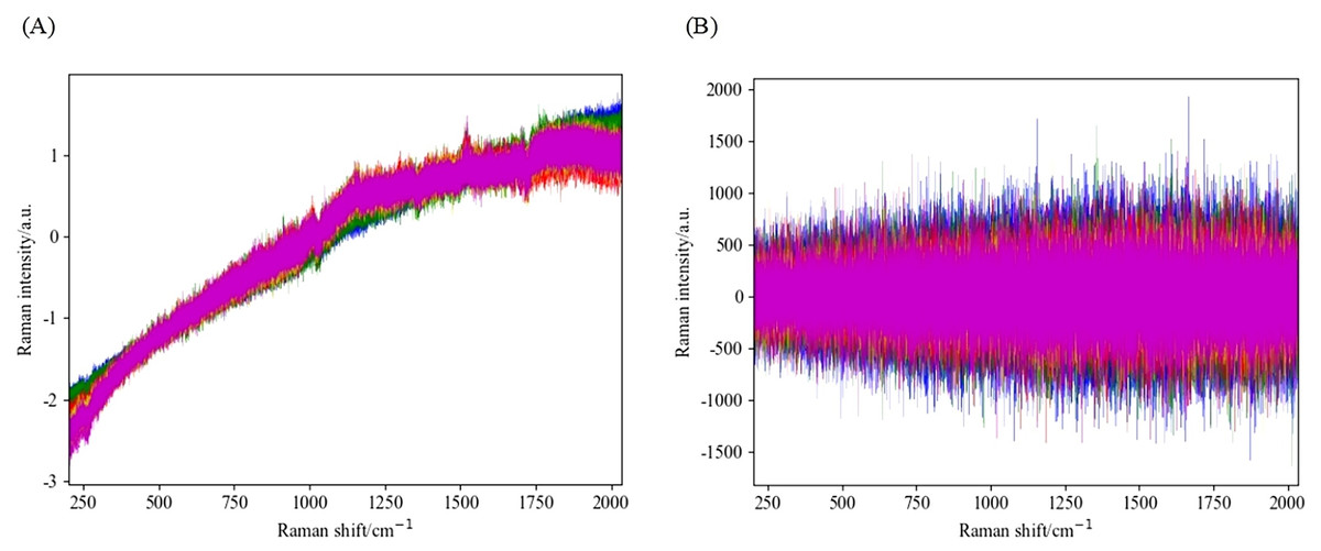
Figure 5: Spectral diagram of WT combined with SNV and first-order derivative processing.
(A) The spectrum of SG and SNV combined processing. (B) The spectrum obtained by combining SG and first derivative processing.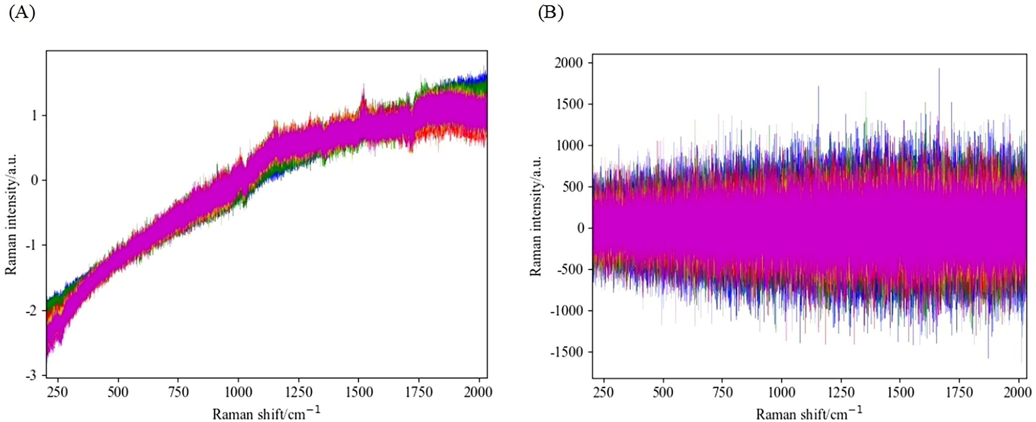
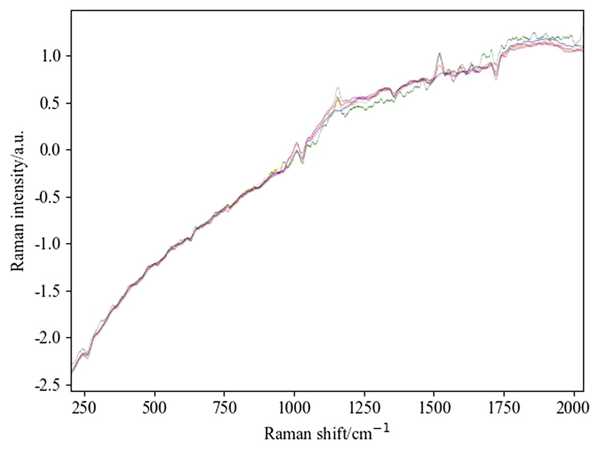
Figure 6: Spectral difference map of pretreated maize in different years.
By observing the preprocessed spectrum, it can be found that the peak information of the processed spectrum is more abundant compared to the original image. Further comparison reveals that the feature peaks presented by the preprocessing method combined with SG are more pronounced compared to the method combined with WT. To evaluate the advantages and disadvantages of these preprocessing methods, this study selected the SVM algorithm as the modeling tool, conducted modeling experiments on four different preprocessing combination methods, and analyzed their accuracy and running time.
According to the data in Table 1, the characteristic peak of the method combined with SG is more significant, which shows obvious advantages in improving the accuracy of the model, resulting in better overall performance. Meanwhile, in terms of running time, the method combined with SG has also shown advantages. Specifically, the combination method of SG and SNV showed an 11% increase in accuracy and a 10 s reduction in running time compared to the combination with first-order derivatives, demonstrating the superior performance of the SG and SNV combination method.
| Preprocessing | Accuracy (%) | Elapsed time (s) |
|---|---|---|
| WT+SNV | 80.21 | 166.43 |
| WT+1Der | 51.67 | 169.55 |
| SG+SNV | 96.69 | 99.53 |
| SG+1Der | 85.32 | 109.31 |
Feature extraction based on spectral data
The establishment of a model is particularly important for accurately predicting the year information of samples. Before building a classification model, it is necessary to extract features from the processed spectral data, that is, convert spectral information into feature vectors. However, if the feature dimension is too large, it will increase the computational complexity and thus affect the classification accuracy. To avoid overfitting, the sample size of the data matrix should be much larger than its feature count to ensure the accuracy of classification performance. Therefore, after data preprocessing, it is necessary to extract features through dimensionality reduction operations. The dimensionality of LDA after dimensionality reduction needs to be smaller than the number of categories. Therefore, in the experiment, the dimensionality reduction parameter of LDA was set to 4, and the 3,315 dimensional spectral data was reduced to a four-dimensional feature vector. Similarly, in the ICA dimensionality reduction method, the number of independent components is set to 10, resulting in a 10 dimensional feature vector. The results are shown in Fig. 7, with the left image showing the 3D graphics reduced by LDA and the right image showing the 3D graphics reduced by ICA. Among them, different colors represent sample data from different years. It can be seen from the figure that after dimensionality reduction, data of the same category are closer, making the overall data more conducive to classification in high-dimensional space.
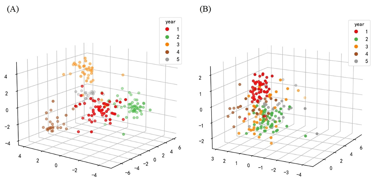
Figure 7: Three dimensional model of data after dimensionality reduction.
(A) The graph after LDA dimensionality reduction. (B) The image after ICA dimensionality reduction.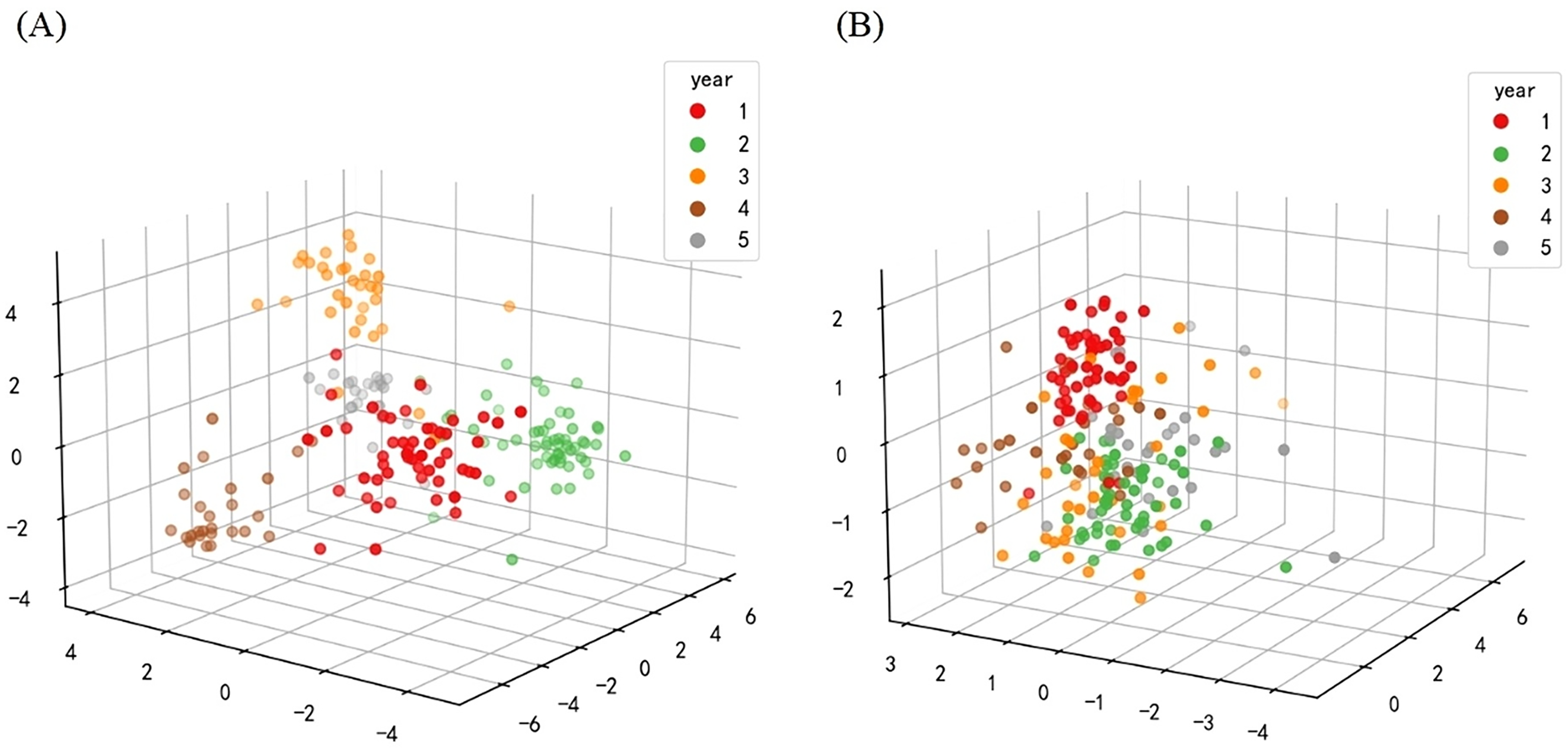
Modeling and analysis based on feature vectors
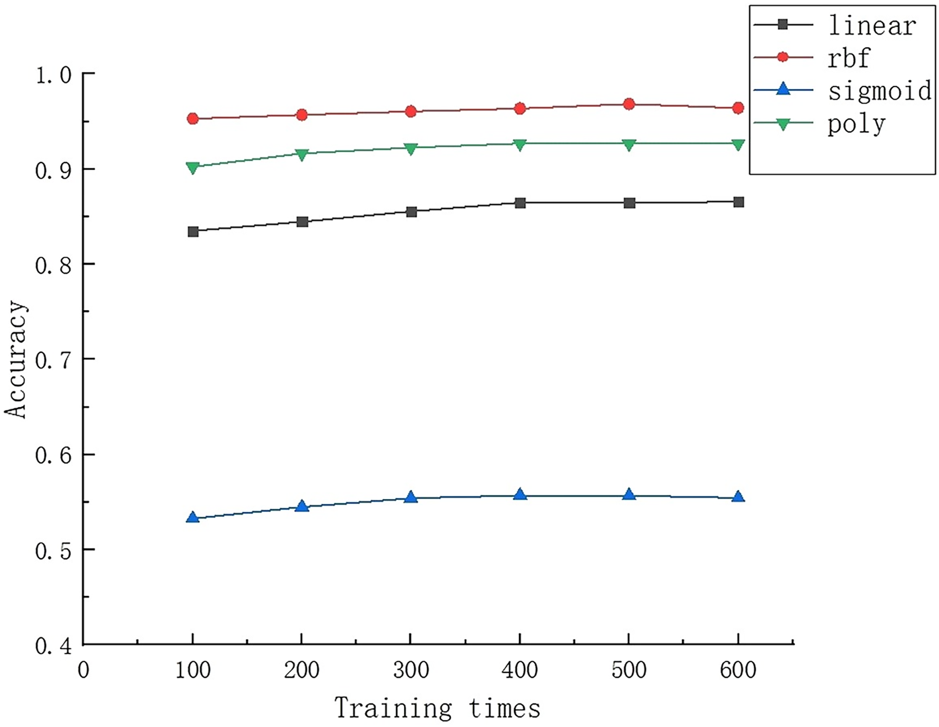
In order to evaluate the performance of different classification models, SVM, RF and KNN classification models were established for training and prediction in the experiment. In the process of establishing SVM models, it is necessary to pay attention to the selection of parameters, especially the selection of kernel functions, as this has a crucial impact on the performance of the model. Through experimental comparative analysis, the results shown in Fig. 8 were obtained. Specifically, the rbf kernel function showed the best performance in the experiment, with an overall accuracy of over 95% for the model. In contrast, the sigmoid kernel function has poor performance, with an accuracy of only 60% or less. It is worth noting that although the sigmoid kernel function may perform well on certain specific datasets, the rbf kernel function is widely used due to its strong locality and ability to handle non-linear separable data, and has also shown good performance on small sample datasets.
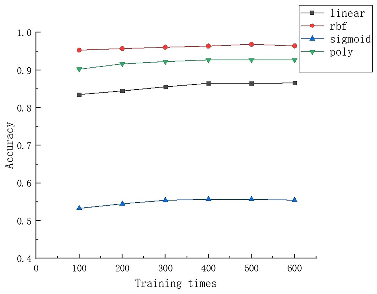
Figure 8: Results of different kernel functions after multiple trainings.
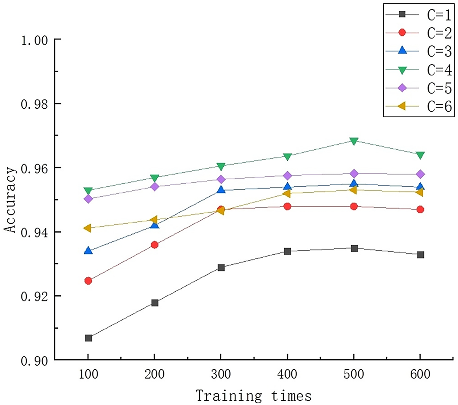
After selecting the rbf kernel function, the setting of the penalty parameter C in the kernel function has a significant impact on overall performance. The C parameter is used to adjust the preference weight between interval size and classification accuracy. Specifically, when the C value is too high, the model is prone to overfitting; When the C value is too small, it is easy to experience underfitting. In order to find the optimal C value, experimental comparative analysis was conducted with different values, and the results are shown in Fig. 9. After careful analysis, it was found that when C = 4, the overall performance of the model was optimal, and the adjustment of interval size and classification accuracy reached the optimal state. A C value that is either too large or too small can lead to a decrease in the overall accuracy of the model.
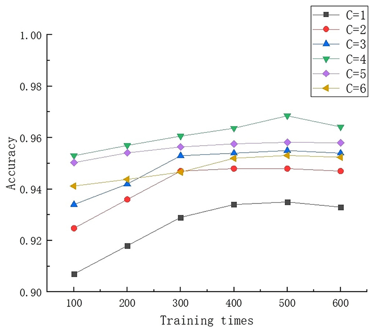
Figure 9: Results of multiple training for different C values.
In the preprocessing stage of spectral data, the method of combining SG with SNV and first-order derivative was adopted. After these preprocessing steps, the spectral data is further processed using two dimensionality reduction techniques, LDA and ICA, to extract feature information. Subsequently, experimental verification was conducted on these feature information using three classification algorithms: KNN, RF, and SVM.
As shown in Table 2, the preprocessing method combining SG and SNV demonstrated higher overall accuracy in subsequent experiments. In terms of dimensionality reduction methods, ICA has shown better performance compared to LDA, with an accuracy improvement of 12%. This improvement may be attributed to the higher dimensionality of features extracted by ICA, which preserves more information that is more conducive to subsequent model classification.
| Preprocessing | Dimensionality reduction | Classification algorithm | Accuracy (%) | Recall (%) | F1-score | Elapsed time (s) |
|---|---|---|---|---|---|---|
| SG+1Der | LDA | KNN | 55.36 | 55.07 | 0.5375 | 140.43 |
| RF | 79.62 | 79.67 | 0.7845 | 186.77 | ||
| SVM | 66.96 | 66.38 | 0.6549 | 137.27 | ||
| ICA | KNN | 74.89 | 75.82 | 0.7454 | 114.33 | |
| RF | 89.72 | 90.10 | 0.8942 | 172.19 | ||
| SVM | 85.32 | 86.20 | 0.8501 | 109.31 | ||
| SG+SNV | LDA | KNN | 79.61 | 79.75 | 0.7865 | 124.57 |
| RF | 84.21 | 84.51 | 0.8359 | 161.32 | ||
| SVM | 80.91 | 81.15 | 0.8039 | 119.05 | ||
| ICA | KNN | 88.96 | 89.68 | 0.8865 | 99.38 | |
| RF | 93.44 | 93.62 | 0.9327 | 155.42 | ||
| SVM | 96.69 | 96.77 | 0.9659 | 99.53 |
In the comparison of classification algorithms, KNN performs relatively poorly. When RF is processed using a combination of SG and first-order derivative (1Der), its performance is slightly better than the other two algorithms, but its running time is relatively long, and the best experimental results have an accuracy rate of less than 90%. In contrast, SVM has the best overall performance, with an accuracy rate of 96.69% and a recall rate of 96.77% under optimal conditions, indicating excellent performance of the model in identifying positive class samples. In addition, the F1 value of SVM reached 0.9659 and the running time was 99.53 s, which is relatively short, indicating that the overall performance of SVM model is better than the other two algorithms.
On this basis, additional experiments were conducted on spectral data, which involved removing the preprocessing and feature extraction steps for SVM classification prediction. After removing the preprocessing part, the accuracy of SVM classification is 90.14%; After removing feature extraction, the accuracy decreased to 80.41%. This indicates that the feature extraction step has a greater impact on the final result, maximizing the removal of irrelevant information and preserving features that effectively distinguish between different years. Meanwhile, appropriate data preprocessing can also effectively improve recognition performance. Figure 10 shows the classification confusion matrix of the feature information obtained after spectral data processing on KNN, RF, and SVM, with the results of KNN, RF, and SVM from left to right. The rows of the matrix represent the true labels, and the columns represent the predicted results, where 0–4 represent the five years from 2014 to 2020. The experiment was conducted multiple times and the average was taken to eliminate randomness, and the confusion matrix was also averaged. Analyzing the confusion matrix, it was found that after preprocessing and feature extraction, SVM had higher individual accuracy for different years than the other two algorithms. Among them, corn from 2015 and 2020, as well as 2018 and 2019, were prone to confusion during SVM classification, which may be due to the similarity of Raman spectroscopy data.
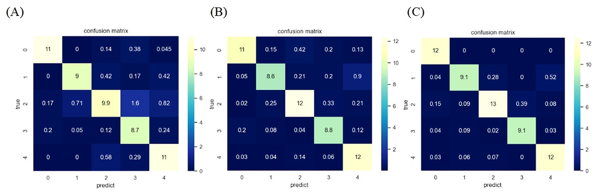
Figure 10: Confusion matrix of SVM algorithm after different preprocessing.
(A) The confusion matrix after KNN classification. (B) The confusion matrix after RF classification. (C) The confusion matrix after SVM classification.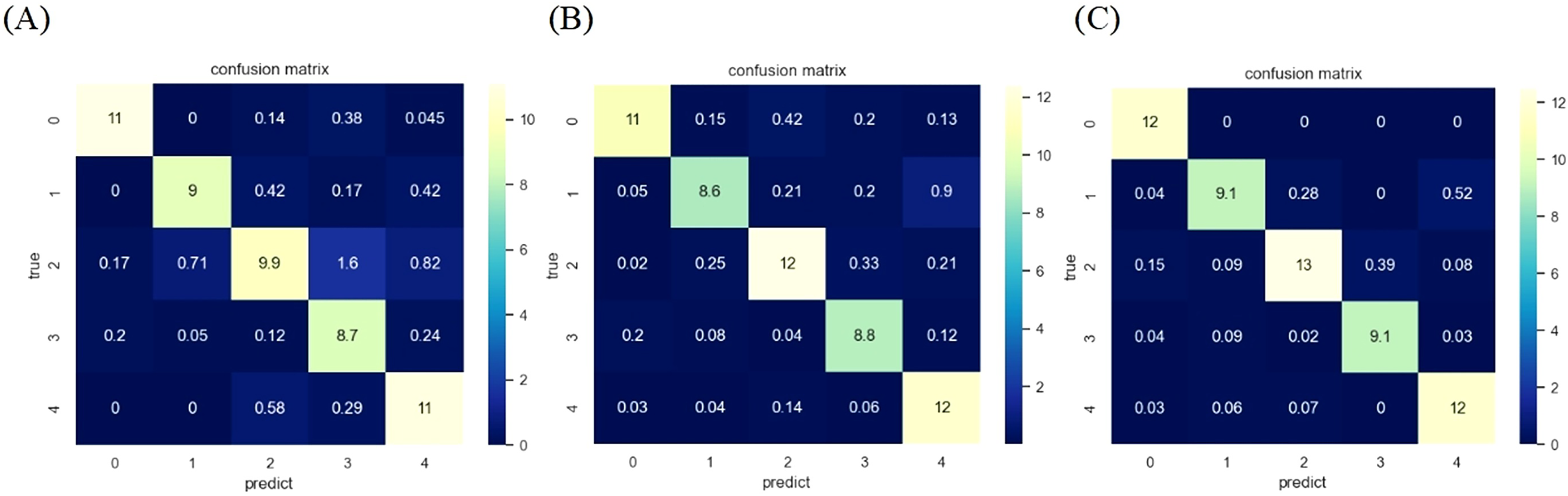
Conclusions
The integration of Raman spectroscopy with machine learning models demonstrates considerable feasibility for corn production year identification. In this study, Raman spectral data of corn samples from five different production years were selected as the classification subjects. Meanwhile, the influence of various preprocessing combinations on classification results was investigated. Experimental results indicated that the combination of SG and SNV exhibited superior processing performance, which could effectively improve classification accuracy. In addition, feature extraction methods have a significant impact on the final results of classification tasks. Specifically, the ICA method has improved accuracy by 12% compared to the LDA method, and the feature information extracted by ICA is more abundant and beneficial for accurate identification of years. While achieving effective feature extraction, ICA also reduces overall complexity and effectively shortens runtime. After multiple experimental verifications, it was found that the overall performance of SVM and random forest classification models is better than that of KNN classification models. Among them, SVM has the best classification effect, achieving an accuracy of 96.69% on the test set, with high recall and F1 value, and relatively short running time. This indicates that the combination of Raman spectroscopy technology and machine learning methods has shown significant feasibility in corn year recognition, the model has good stability under the conditions of different samples, and it is feasible to use the current model to classify different kinds of corn. providing new ideas for corn related detection and references for subsequent research.