TransGraphNet: robust detection of malicious encrypted network traffic via transformer and graph neural models

Qiang Shi; Dacheng Shi; Liukun He; Qingjun Xiao; Liang Zheng; Jun Ma; Jingdong He; Qifan Zhang

doi:10.7717/peerj-cs.3353

TransGraphNet: robust detection of malicious encrypted network traffic via transformer and graph neural models

Qiang Shi¹, Dacheng Shi¹, Liukun He¹, Qingjun Xiao ^1,2, Liang Zheng¹, Jun Ma¹, Jingdong He¹, Qifan Zhang¹

1School of Cyber Science and Engineering, Southeast University, Nanjing, Jiangsu, China

2Purple Mountain Laboratories, Nanjing, Jiangsu, China

DOI: 10.7717/peerj-cs.3353

Published: 2025-11-14
Accepted: 2025-10-09
Received: 2025-04-25

Academic Editor: Giovanni Angiulli

Subject Areas: Algorithms and Analysis of Algorithms, Artificial Intelligence, Computer Networks and Communications, Security and Privacy, Neural Networks
Keywords: Malicious encrypted traffic detection, Traffic obfuscation, Graph attention network, BERT-based transformer model, Spatial-Temporal feature fusion

Copyright: © 2025 Shi et al.
Licence: This is an open access article distributed under the terms of the Creative Commons Attribution License, which permits unrestricted use, distribution, reproduction and adaptation in any medium and for any purpose provided that it is properly attributed. For attribution, the original author(s), title, publication source (PeerJ Computer Science) and either DOI or URL of the article must be cited.

Cite this article: Shi Q, Shi D, He L, Xiao Q, Zheng L, Ma J, He J, Zhang Q. 2025. TransGraphNet: robust detection of malicious encrypted network traffic via transformer and graph neural models. PeerJ Computer Science 11:e3353 https://doi.org/10.7717/peerj-cs.3353

The authors have chosen to make the review history of this article public.

Abstract

As encrypted network traffic becomes more prevalent, cybercriminals increasingly conceal their malicious activities within encrypted session contents. Traditional methods for detecting malicious encrypted traffic focus on inspecting the plaintext payload during the Transport Layer Security (TLS) handshake phase and analyzing directed Internet Protocol (IP) packet length sequences during the subsequent encrypted transmission phase. However, these methods often have high miss-detection rates in real-world scenarios. For example, attackers employ active traffic obfuscation techniques, such as forging TLS Service Name Indicators (SNI) and certificates to evade detection, while network environments introduce passive obfuscation through packet sequence perturbations. To address these challenges and improve detection robustness, we propose transGraphNet, a novel framework that integrates multi-granularity features from both the packet-length sequences within individual network connections and the flow-relation graphs representing interactions among multiple connections. For each session between a pair of client-server IP hosts, we partition its involved flows into session windows using an adaptive session window algorithm, and then capture concurrency and trigger relationships between their transmitted flows by constructing an Adaptive Sliding-Window Flow-level burst Graph (AFG). Unlike prior methods such as FG-Net, which constructs a flow-relation graph for each client host, our TransGraphNet groups the flows within the same client-server session and with proximate start times into a session window, which is used as a more fine-grained target for traffic classification. Additionally, for each five-tuple flow, we apply the packet length standardization using an enhanced Power Law Division (PLD) algorithm to mitigate time-series noise caused by passive obfuscation. We also integrate packet length sequence modeling and capture its long-range dependencies through a transformer-GNN model, thereby enhancing its representational power. Specifically, for each flow, temporal statistical features are extracted using Convolutional Neural Network (CNN), while long-range dependencies within the packet length sequence are captured via Bidirectional Encoder Representations from Transformers (BERT). These flow representations serve as node features in the AFG, where a graph attention network is employed to propagate and aggregate information across the graph’s topology. The resulting AFG representation is then used for malicious encrypted traffic detection. Extensive experiments on the traffic dataset with obfuscation show that TransGraphNet outperforms state-of-the-art methods such as FG-Net, ET-BERT, and GraphDApp, improving accuracy by 11%, 5.4% and 6.8%, respectively.

Introduction

Nowadays, network traffic encryption has become essential to ensure the secure transmission of internet data. While encrypted communication effectively protects the sensitive information of legitimate users, it also allows cybercriminals to conceal their malicious activities. According to a report by Zscaler (2023), 85.9% of network threats are launched over encrypted channels, with malicious encrypted traffic accounting for 78.1% of all attack attempts. As a result, accurately detecting malicious network traffic within encrypted communications has become a critical challenge in cybersecurity.

To detect malicious encrypted traffic, network intrusion detection systems (NIDS) often utilize deep packet inspection (DPI) to examine the plaintext messages exchanged between a client and a server during the Transport Layer Security (TLS) handshake, a critical phase where cryptographic parameters are negotiated before actual data encryption begins. This analysis focuses on specific fields within the handshake protocol that can reveal suspicious intent (Keshkeh et al., 2021), such as server name indicators (SNI) that might point to untrusted or known malicious domains, certificate chains that may contain invalid, self-signed, or revoked certificates linked to malicious entities, and cipher suites that deviate from standard security best practices.

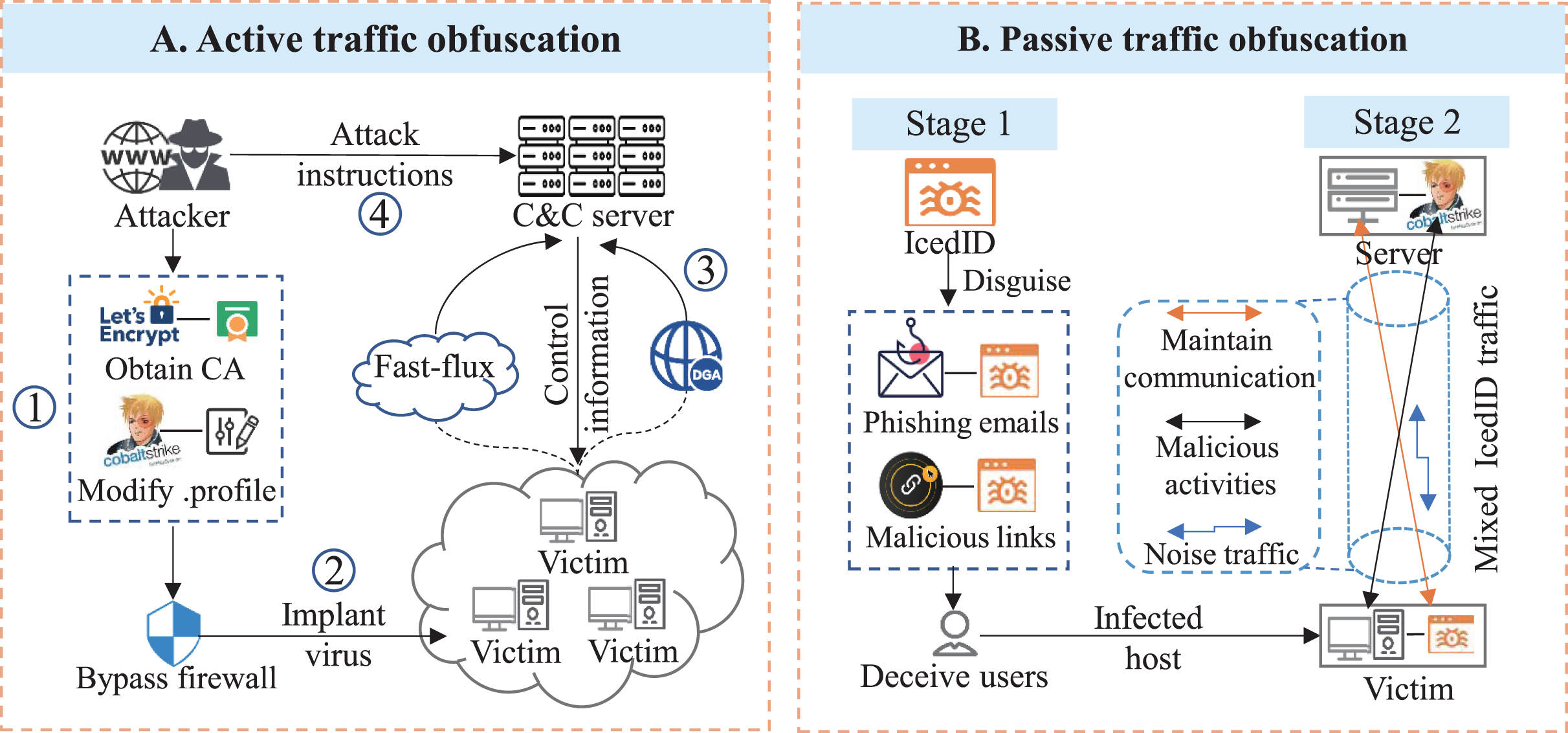
To evade deep packet inspection, attackers often adopt active obfuscation techniques (CobaltStrike, 2024) by forging TLS-related parameters or customizing communication behaviors (Lee & Jin, 2021). For instance, as shown in Fig. 1A, attackers can obtain legitimate certificates from trusted certificate authorities (e.g., Let’s Encrypt) and use penetration test tools such as CobaltStrike to configure HTTPS Beacons, for example, modifying heartbeat intervals, ports, and TLS certificate fields (CobaltStrike, 2024). These behaviors produce malicious encrypted traffic that closely mimics legitimate traffic in terms of TLS protocol features, certificate structures and beaconing intervals (The DFIR Report, 2021), making it difficult for firewalls to distinguish. Traditional rule-based or statistical approaches based on TLS certificate features (Bastos et al., 2019; Dai et al., 2019), along with deep learning models that rely on handshake payloads (Bayat, Jackson & Liu, 2021; Sun et al., 2022), are often misled by such sophisticated obfuscation.

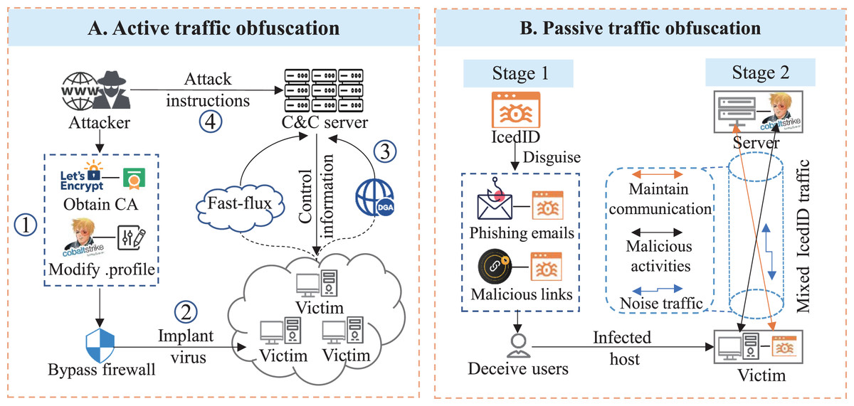
Figure 1: Typical network attacks, and two types of traffic obfuscation in real-world environments: (A) Attackers compromise intranet hosts, communicate with C&C servers over encrypted connections, and use active traffic obfuscation techniques to bypass firewalls; (B) Attackers send phishing emails to trick users into downloading IcedID malware, whose traffic is passively obfuscated by network environments.

Download full-size image

DOI: 10.7717/peerj-cs.3353/fig-1

Following the TLS handshake, a sequence of encrypted packets is transmitted, with payloads rendered unreadable to traditional DPI techniques. Advanced NIDS can still identify anomalies by leveraging the patterns in packet lengths and timing during this phase, an approach known as “traffic fingerprinting”. For example, as shown in Fig. 1A, Remote Access Trojans (RATs) implanted by attackers regularly exchange IP packets with Command and Control (C&C) servers to transmit heartbeat signals or fetch new commands, creating behavioral patterns that can be monitored by firewalls (Piet, Anderson & McGrew, 2018). As a result, in recent years, an increasing number of detection methods have focused on learning temporal patterns within IP packet transmissions of five-tuple flows, such as directed packet length sequences and inter-packet arrival times (Sirinam et al., 2018; Lotfollahi et al., 2020; Liu et al., 2019).

However, in real-world scenarios, both active and passive traffic obfuscation contribute substantially to the high miss-detection rates of existing approaches. Passive obfuscation can occur naturally under adverse network conditions, such as packet loss, fragmentation, and latency variations, which perturb the order, timing, and length of IP packet sequences. These disturbances degrade the effectiveness of detection models that depend on temporal features (Yang et al., 2023). An example is shown in Fig. 1B: an attacker sends phishing emails to deliver IcedID malware, which maintains persistent encrypted communication with a C&C server. Later, a second-stage tool (e.g., CobaltStrike) is deployed for activities such as data exfiltration. In such multi-stage attacks, captured CobaltStrike traffic is often intermixed with IcedID traffic (The DFIR Report, 2021), distorting temporal patterns and hindering accurate detection. In addition, the packet length sequences of these flows are obfuscated by the network environment, which introduces perturbations in the order, timing, and length of IP packets (Yang et al., 2023). This makes it difficult for models that rely on temporal features to accurately capture the underlying patterns of malicious traffic.

We refer to the above naturally occurring disturbances as passive traffic obfuscation. In contrast, active traffic obfuscation, including mimicry attacks, traffic morphing, padding, and random delays, deliberately alters packet sequences to make malicious flows resemble benign ones, thereby breaking the semantic patterns that time-series models aim to learn. In summary, both active and passive obfuscation corrupt key features within five-tuple flows, including TLS handshake features and temporal packet sequence patterns, rendering detection methods that rely solely on such features vulnerable to deception (The DFIR Report, 2021).

To address this, it is critical to enhance the robustness of detection systems by leveraging features that attackers or environmental factors cannot easily modify (Yonghao, Hao & Xiaoqing, 2023). One such underutilized feature is the interaction patterns among multiple five-tuple connections transmitted between a pair of IP hosts. For example, attackers cannot easily obfuscate the bursty traffic behaviors formed by flows transmitted concurrently within a short attacking period (Oudah et al., 2019). The multiple flows between a client and a server can be modeled as a flow-relation graph, in which each vertex represents a five-tuple connection, and edges denote the concurrency and trigger relationships between these connections.

While existing methods, such as FG-Net (Jiang et al., 2022) and Darknet Graph Neural Networks (DGNN) (Zhu et al., 2023), also utilize flow relation graphs, their performance remains insufficiently optimized. This is primarily because flow relation graphs only capture coarse-grained relationships, such as concurrency or sequencing between flows, which are insufficient for achieving high detection accuracy. The effectiveness of graph-based models heavily depends on the quality of vertex features, particularly those derived from five-tuple flows (e.g., statistical features, handshake metadata, or IP packet sequences). However, prior work often neglects proper preprocessing of these features. For instance, IP packet lengths, which are susceptible to environmental noise (Li et al., 2023), require standardization, a step overlooked by many existing methods. Furthermore, they fail to fully exploit temporal packet length patterns. Instead of employing more effective long-range dependency models like Transformers (Zhao et al., 2025), they typically rely on CNNs, which are better suited for short-term dependencies. Additionally, the granularity of flow relation graphs in previous methods is insufficient. Most previous studies group flows by client IP or MAC address and partition the time axis into fixed windows to construct graphs (Yang et al., 2024a). This strategy may miss critical interaction patterns when flows are unevenly distributed over time axis, and a finer-grained approach, such as grouping flows by client-server sessions, could better capture malicious behavior.

To address the challenge of detecting malicious encrypted traffic under both passive and active obfuscation, we propose TransGraphNet, a robust detection framework that integrates multi-granularity traffic features through spatial-temporal modeling. TransGraphNet consists of three core modules:

Packet length noise mitigation module: This module addresses noise in IP packet sequences caused by passive obfuscation using an enhanced Power Law Division (PLD) algorithm. It standardizes packet lengths within five-tuple flows (Yang et al., 2023; Li et al., 2023) in three steps: (i) identifying the top-k most frequent packet lengths; (ii) mapping packet lengths with small deviations to their nearest high-frequency values; and (iii) for larger deviations, mapping to the nearest regular interval. This process effectively suppresses noise while preserving essential traffic characteristics.
Flow relation graph construction module: This module constructs Adaptive sliding-window Flow-level burst Graphs (AFGs). It first groups flows by client-server sessions, then segments each session’s flows into adaptive session windows. For each window, it builds an AFG that captures concurrency and trigger relationships among flows, enhancing robustness by modeling inter-flow dynamics.
Spatial-temporal feature fusion module: This module integrates spatial and temporal features using a hybrid Transformer-GNN model to enhance representation capacity and detection performance (Diao et al., 2023; Yang et al., 2024a; Liu et al., 2023). Each flow is represented by three components: (i) statistical features compressed by a CNN; (ii) IP packet length sequence; and (iii) packet inter-arrival time sequence. The latter two capture temporal dynamics, with long-range dependencies modeled by BERT. The resulting flow-level embeddings serve as node features in the Adaptive Flow Graph (AFG), where a Graph Attention Network (GAT) propagates and aggregates information across the graph structure. By jointly modeling intra-flow and inter-flow features, TransGraphNet effectively mitigates the effects of traffic obfuscation and improves robustness in malicious encrypted traffic detection.

The main contributions of this article are summarized as follows. The dataset and source code are publicly available at https://github.com/TransGraphNet/TransGraphNet.

We improve the model’s robustness to malicious encrypted traffic with passive obfuscation by introducing an improved Power Law Division (PLD) algorithm. Unlike traditional PLD methods that focus solely on top-k high-frequency values, we adopt a hybrid discretization strategy: it standardizes packet lengths by combining the most frequent values within each traffic class with regularly spaced values (e.g., every 7 bytes). This design enables better preservation of dominant traffic characteristics while ensuring coverage of rare but potentially informative patterns, thus enhancing robustness against noises.
We propose a novel AFG to model the behavior of client-server two-tuple session windows by capturing interactions among five-tuple flows. Unlike prior methods that rely on fixed time windows or client IPs (Jiang et al., 2022; Yang et al., 2024a), we group flows within the same client-server session and with proximate start times into a session window, which is used as a more fine-grained target for traffic classification. Then, AFG represents each session window as a time-ordered sequence of bursts, where flows within the same burst are concurrently transmitted for a shared application-level purpose, and successive bursts exhibit trigger relationships.
We propose a transformer-GNN hybrid model to capture both the temporal and spatial features of an AFG. Specifically, CNN and BERT are used to extract the temporal statistical and time-series features of five-tuple flows (i.e., AFG vertices), while a Graph Attention Network (GAT) captures spatial interactions among flows. This spatial-temporal feature fusion enhances the model’s representational capacity.
Experimental results demonstrate that TransGraphNet effectively detects malicious encrypted traffic with obfuscation in the Malware-Traffic-Analysis (MTA) (Duncan, 2024) dataset, achieving state-of-the-art performance. Moreover, the model demonstrates strong generalization ability. It remains robust on standard encrypted traffic datasets without obfuscation, such as CIC-IoT-2023 and Stratosphere.

Related work

In this section, we classify existing traffic classification methods based on the features and behavioral granularity they capture from encrypted traffic. We review the limitations of these existing approaches and highlight the key contributions of our proposed TransGraphNet framework.

TLS handshake inspection methods

In TLS-based encrypted network traffic, an initial handshake phase precedes the transmission of encrypted payloads. For TLS 1.2 and earlier versions, plaintext features, such as certificate information, cipher suite lists, and Service Name Indicators (SNI) fields, can be extracted from the handshake phase. For example, TLSmell (Weng et al., 2021) proposed a detection framework for malicious HTTPS traffic that constructs four-tuple flows (source IP, destination IP, destination port, and protocol) and correlates three types of Zeek logs (conn.log, ssl.log, and x509.log). It extracts 33 features categorized into connection indicators, TLS indicators, and certificate indicators, and employs classifiers such as SVM, CNN, and LSTM to improve detection performance. Lokoč et al. (2016) introduced features such as handshake duration and the interval between consecutive TLS requests, using a KNN model with the MIINDEX metric for malicious traffic detection. Similarly, Dai et al. (2019) proposed a plaintext vector-based feature selection method that extracts information from the handshake and certificate phases and applies mutual information to refine the feature set, thereby enhancing detection accuracy. However, these detection methods are highly susceptible to active traffic obfuscation, in which attackers manipulate handshake parameters or forge TLS certificates to evade inspection (Weng et al., 2021; Dai et al., 2019).

Flow-level statistical feature-based methods

To overcome the limitations of TLS handshake inspection methods, subsequent research has shifted focus to analyzing encrypted payloads during the transmission phase. These methods typically extract statistical features from the packet length sequences of individual flows, which are more robust to active obfuscation. Specifically, they rely on handcrafted statistical features such as packet count, average packet size, inter-arrival time, flow duration, and byte statistics. For example, Alshammari & Zincir-Heywood (2011) used only packet header and flow-level statistical features, omitting any payload-related information. AppScanner (Taylor et al., 2016) applied GINI importance to evaluate feature relevance, selecting the top 40 statistical features to train a random forest classifier. ADABIND (Al-Naami et al., 2016) introduced new features by modeling the sizes of adjacent upload/download bursts and the time taken for burst transmission, using SVM for classification. In contrast to single-model approaches, Feature Fusion Fingerprinting (FFP) (Shen et al., 2019) used an ensemble of classifiers, including KNN, random forest and SVM, to improve accuracy by leveraging the strengths of each model.

Although these methods effectively detect various types of traffic using general statistical features (Alshammari & Zincir-Heywood, 2011; Taylor et al., 2016; Shen et al., 2019), they are not specifically tailored for encrypted traffic. The coarse granularity of their feature sets limits their ability to capture subtle behavioral patterns inherent in encrypted flows. To address these limitations, our proposed TransGraphNet extracts 103 multi-granularity temporal statistical features at both the packet and flow levels to construct more expressive representations. In addition, we incorporate deep learning models that directly process raw IP packet sequences to further enhance detection performance.

Raw IP packet sequence-based methods

These methods move beyond handcrafted statistical features by modeling network flows as sequences of raw IP-layer attributes (e.g., packet lengths, directions, and arrival times). They typically leverage time-series architectures such as RNNs, CNNs or Transformers to capture temporal dependencies. While offering greater flexibility and reduced reliance on expert-defined features, such methods are often sensitive to noise and obfuscation in packet sequences. For example, DF (Sirinam et al., 2018) proposed a deep fingerprinting model that uses packet direction sequences as input and applies CNNs to identify Tor traffic. To incorporate additional features, FS-Net (Liu et al., 2019) employs multi-layer bidirectional gated recurrent units in both its encoder and decoder layers to capture temporal dependencies within packet length sequences. It integrates a reconstruction mechanism, where the decoder reconstructs the input sequence to enhance feature effectiveness, and combines encoder-based and decoder-based features via a dense layer for classification. MGREL (Yonghao, Hao & Xiaoqing, 2023) adopts a dual-granularity approach by dividing encrypted sessions into TLS handshake fields and packet sequences. It extracts local behavioral semantics from handshake fields using word embeddings with positional prefixes, multi-head attention, and Bidirectional Long Short-Term Memory (BiLSTM), while global semantics are obtained from packet sequences using Long Short-Term Memory (LSTM) with spatiotemporal state tracking. These features are fused to achieve superior detection performance over state-of-the-art baselines. However, CNN- and RNN-based models often struggle to capture long-range dependencies, resulting in incomplete sequence representations and degraded detection accuracy.

With the growing popularity of large language models (LLMs) and their strength in modeling long-range dependencies, researchers have increasingly explored their applications in network traffic analysis. For instance, Encrypted Traffic Bidirectional Encoder Representations from Transformer (ET-BERT) (Lin et al., 2022) introduces a Transformer-based pretraining framework for encrypted traffic classification. It converts the payload bytes of a flow’s packets into language-like tokens via a Datagram2Token procedure, and learns contextualized representations through two traffic-specific pretraining tasks: Masked BURST Modeling and Same-Origin BURST Prediction. This approach achieves state-of-the-art performance on multiple benchmarks. To integrate richer feature sets, PETNet (Yang et al., 2024b) proposes a plaintext-aware encrypted traffic detection network targeting Cobalt Strike HTTPS traffic. It jointly analyzes TLS handshake fields and packet payload bytes using a Transformer-based architecture. These studies highlight the significant potential of leveraging time-series representations and Transformer models to improve encrypted traffic detection (Yang et al., 2024b; Lin et al., 2022).

Our proposed TransGraphNet also uses BERT to capture long-range dependencies and complex temporal patterns in packet-level time series data, providing rich information for encrypted traffic classification. While prior works like ET-BERT and PETNet leverage Transformer-based architectures to model packet-level time series, they primarily focus on intra-flow features and do not capture inter-flow relationships. In contrast, our TransGraphNet integrates both intra-flow packet sequences and inter-flow relationships through a flow-relation graph, enabling a more comprehensive understanding of encrypted traffic behavior. This dual focus enhances the model’s robustness against both active and passive obfuscation techniques.

Flow interaction graph-based methods

Malicious traffic often exhibits distinctive behavioral patterns, such as bursty growth or periodic fluctuations, which reflect rich interactions among network flows. To capture these high-level semantics, typically more resilient to obfuscation, recent approaches model inter-flow relationships, such as concurrency and causality dependencies, using one- or two-tuple session-level graph representations. For example, FG-Net (Jiang et al., 2022) constructs a flow relationship graph for each client IP host, where vertices are network flows with packet-level (e.g., packet size, time interval) time sequences. It captures two kinds of flow-level relationships: concurrency (flows in the same burst with start time differences $< δ$ ) and trigger (linking previous burst’s tail to next burst’s head/tail). Using GNN with attention for feature propagation, it excels in mobile app identification, especially with ambiguous traffic and against traffic concept drift. Since FG-Net applies CNN to packet time sequences, it struggles with extracting long-range features. To address this, Lakshmanan et al. (2024) applied a Graph Neural Network (GNN)-Transformer model for cyber threat detection in smart grids: GNN extracts spatial features based on power system topology, while the Transformer encoder captures long-range temporal dependencies by self-attention. Govindarajan & Muzamal (2025) proposed a cloud intrusion detection framework. It combines GNNs to capture network topological relationships, Transformer autoencoders to learn sequential patterns in traffic, and contrastive learning to enhance feature discrimination. It shows high robustness in complex, imbalanced network environments.

Traditional flow relation graph-based methods, such as FG-Net (Jiang et al., 2022) and DGNN (Zhu et al., 2023), exhibit several limitations that constrain their detection performance. First, they frequently overlook the standardization of IP packet sizes, which are highly susceptible to environmental noise (Li et al., 2023), thereby introducing instability into model inputs. Second, although they construct flow-relation graphs to capture interactions, they tend to underutilize the temporal packet length features within individual flows. Most rely on shallow temporal models, typically CNNs, which capture only local patterns and lack the capacity to model long-range dependencies, an area where Transformer-based models have demonstrated clear advantages (Zhao et al., 2025). Third, these methods typically segment traffic using fixed time windows, which can result in information loss when flow distributions are uneven over time. To address this, we design a dynamic sliding window algorithm that groups flows with proximate start times within the same client-server session, forming a more fine-grained and context-aware session window for classification. In contrast, our TransGraphNet integrates the three components (i.e., packet length standardization, dynamic-window flow relation graph construction, and spatial-temporal feature fusion model combining CNN, Transformer and GAT), to enhance robustness against traffic obfuscation.

Previous studies have also explored packet-level interaction graphs for encrypted traffic analysis, but they do not investigate flow-level interaction graphs as we do. GraphDApp (Shen et al., 2021) pioneered the use of Traffic Interaction Graphs (TIG), where individual packets are modeled as vertices, and GNNs are applied to capture complex inter-packet relationships, enabling accurate identification of decentralized application (DApp) traffic. EC-GCN (Diao et al., 2023) introduced a multi-scale GCN framework that leverages traffic metadata to construct hierarchical graph representations, allowing protocol-agnostic analysis by dynamically learning both local and global interaction patterns. Higher-Interaction-Graph Encrypted Classifier (HIGEC) (Hu et al., 2024) further advanced this paradigm with Cyclic Interaction Graphs (CIG), which explicitly model bidirectional dependencies between packets using cyclic graph structures, enhancing the capture of temporal and causal relationships in encrypted flows. Most recently, MTSecurity (Yang et al., 2024a) constructs a Malicious Traffic Interaction Graph with packets as vertices (nine-dimensional features) and edges for intra/inter-burst connections. It fuses GNN extracted graph features and Transformer-learned temporal features from privacy-preserving byte data, achieving high accuracy in encrypted malicious traffic classification.

Summary of limitations of existing methods

Challenges under traffic obfuscation: Methods relying on TLS certificate features are vulnerable to active obfuscation techniques, such as forged certificates and SNI fields. Meanwhile, IP packet sequence-based methods are often disrupted by noisy sequences introduced through passive obfuscation.
Loss of flow interaction information: Many graph-based approaches segment traffic using fixed static time windows, which may fail to capture meaningful interactions between temporally correlated flows, leading to incomplete or fragmented graph structures.
Insufficient fusion of spatial-temporal features: Existing models typically focus on either intra-flow packet sequences or inter-flow relationships, without effectively integrating both spatial and temporal dimensions. Moreover, long-range dependencies within flows are often underrepresented, limiting the model’s ability to capture comprehensive flow behavior patterns.

Methodology

An overview of model design

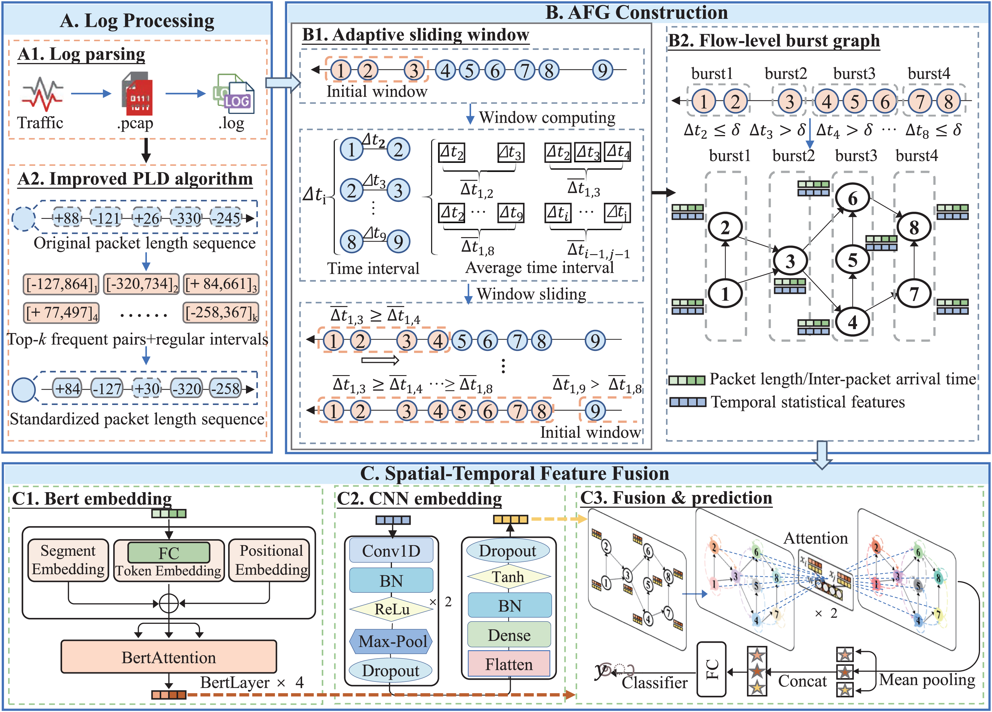
Given the challenges posed by obfuscated malicious encrypted traffic, as discussed in the Introduction, and the limitations of existing methods, as outlined in the Related Work, we propose TransGraphNet. As illustrated in Fig. 2, TransGraphNet adopts a multi-module framework, described as follows.

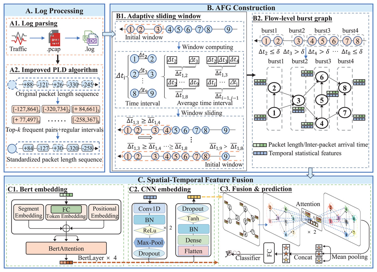
Figure 2: Framework of TransGraphNet with three major phases: (A) Network raw data preprocessing to generate a standardized packet-length sequence for each flow; (B) Adaptive sliding-window Flow-level burst Graph (AFG) construction; (C) Spatial-temporal feature fusion using BERT, CNN, and GNN models.

Download full-size image

DOI: 10.7717/peerj-cs.3353/fig-2

First, we perform a brief analysis of TLS protocol-related features and analyze their robustness against active traffic obfuscation. Based on the findings, we select a combination of per-flow statistical features, IP packet timing sequences, and flow-level interaction features as model inputs. To mitigate the impact of sequence noise introduced by passive obfuscation (Li et al., 2023), we enhance the Power Law Division (PLD) algorithm to standardize packet length sequences, as illustrated in Fig. 2A.

Second, to better capture the dynamic behaviors of malicious traffic, we propose an Adaptive Sliding Window (ASW) algorithm. This algorithm dynamically adjusts the window size based on traffic variations, as shown in Fig. 2B1, effectively capturing dynamic behaviors and addressing the issue of missing interaction information under fixed time windows (Jiang et al., 2022; Yang et al., 2024a). Building on this, as shown in Fig. 2B2, we construct a Flow-Level Burst Graph to represent and learn the concurrent and trigger relationships between encrypted flows, thereby introducing spatial features to mitigate the impact of active traffic obfuscation.

Finally, as illustrated in Fig. 2C, for spatial-temporal feature fusion, we encode temporal statistical features using a CNN, while a BERT model captures long-range dependencies and complex temporal patterns in packet length sequences (Lin et al., 2022). These representations are embedded into the graph vertices and propagated through a GAT, producing a global session-window-level representation for robust classification of malicious encrypted traffic.

For ease of reference, the symbols frequently used in this section are summarized in Table 1.

Table 1:

Mathematical notations frequently used throughout this article.

Symbol	Description
$G (V, E)$	Flow-level burst graph. V is the set of flows (vertices), and E is the set of edges. An edge between two flows $f_{i}$ and $f_{j}$ (i.e., $(f_{i}, f_{j}) \in E$ ) indicates either a concurrent relationship or a trigger relationship.
$P k t L e n (\cdot)$	Packet length extraction function. For a packet $p$ , $P k t L e n (p)$ returns its length in bytes, multiplied by $+ 1$ if $p$ is transmitted from client to server, and $- 1$ if opposite.
$L^{x}$	Complete packet-length frequency distribution for traffic class $x$ . This list contains all distinct packet lengths observed in class $x$ , sorted in descending order by frequency. Formally, $L^{x} = [(ℓ_{j}^{x}, v_{j}^{x})] \|_{j = 1}^{n^{x}}$ , where $ℓ_{j}^{x}$ and $v_{j}^{x}$ are the packet length and packet length frequency with the $j$ -th highest frequency in class $x$ (and $n_{x}$ is the total number of distinct lengths).
${\tilde{L}}^{x}$	Truncated packet length frequency distribution list for class $x$ , containing the top- $k$ most frequent packet lengths and their corresponding frequencies in $L^{x}$ .
$d i s t (p_{i}, {\tilde{L}}^{x})$	Distance between the packet length $P k t L e n (p_{i})$ and the closest value in the list ${\tilde{L}}^{x}$ .
$Δ τ$	Threshold for standardization. If $d i s t (p_{i}, {\tilde{L}}^{x}) \leq Δ τ$ , the packet length is rounded to the closest value in ${\tilde{L}}^{x}$ . Otherwise, it is rounded to the nearest multiple of $Δ τ^{'}$ .
$Δ τ^{'}$	Regular interval for packet length standardization, which is set to 7 by default.
$S t d P k t L e n^{x} (p_{i})$	Packet length standardization function for a traffic class $x$ . Given a packet $p_{i}$ , this function maps its length $P k t L e n (p_{i})$ to the nearest high-frequency length in the top- $k$ packet length list ${\tilde{L}}^{x}$ , if the distance $d i s t (p_{i}, {\tilde{L}}^{x})$ is within a tolerance $Δ τ$ . Otherwise, it rounds $P k t L e n (p_{i})$ up to the nearest multiple of threshold $Δ τ^{'}$ , i.e., $Δ τ^{'} ⌈ \frac{P k t L e n (p_{i})}{Δ τ^{'}} ⌉$ .
$W_{t}$	Adaptive sliding window starting at time $t$ . It collects all flows whose timestamps lie in the interval $[t, t + Δ T]$ . Within this window, flows that are closely spaced in time (i.e., inter-flow interval $Δ t_{i} \leq δ$ ) are grouped into bursts. These bursts form the basis for constructing the flow-relation graph $G (V, E)$ , where flows are connected if they occur within the same burst.
$Δ T_{i}$	Adaptive window duration (width) for $W_{t}$ , which is dynamically updated according to $Δ T_{i} = f_{i} . t s - W_{t} [1] . t s$ , when the new flow $f_{i}$ is going to be inserted into $W_{t}$ .
$Δ t_{i}$	Time interval between the start of the $i$ -th flow and the $(i - 1)$ -th flow (in chronological order). If $t_{i - 1}$ and $t_{i}$ are the start times of flows $f_{i - 1}$ and $f_{i}$ , then $Δ t_{i} = t_{i} - t_{i - 1}$ .
${\bar{Δ t}}_{i, j}$	Average inter-flow time between flows with start times from $t_{i}$ to $t_{j}$ , defined as ${\bar{Δ t}}_{i, j} = \frac{1}{j - i} \sum_{k = i + 1}^{j} (t_{k} - t_{k - 1}) = \frac{1}{j - i} (t_{j} - t_{i})$ . It represents the mean time interval between consecutive flows within the sub-window $[i, j]$ of the current window $W_{t}$ .
$δ$	Time threshold for burst detection. Two flows are considered part of the same burst (and thus linked in G) if their inter-arrival time $Δ t_{i}$ is below $δ$

DOI: 10.7717/peerj-cs.3353/table-1

Network traffic feature selection and preprocessing

Feature analysis and selection

Nowadays, malware typically uses the TLS protocol for encrypted communication, which consists of two main phases. The first phase is the handshake, where the client and server negotiate cryptographic algorithms, establish shared keys, and perform certificate verification (Yang et al., 2024b). The second phase involves encrypted data transmission, where data is transmitted in ciphertext. In the handshake phase, the payloads can be parsed into semantically explicit meta-features, including IP addresses, port numbers, SNI fields, certificate chain fingerprints, and other certificate-related information. However, penetration testing tools (e.g., CobaltStrike) can leverage active traffic obfuscation techniques such as DGA algorithms, custom communication configurations, or forged certificates (Wang et al., 2023), rendering this information unreliable. Directly feeding these features into the model may lead to misclassification.

Therefore, we discard certificate and TLS protocol features from encrypted traffic and instead focus on exploring multi-granularity features at the packet, intra-flow, and inter-flow levels. These features include per-flow statistical metrics (such as the minimum, maximum, average and sum of packet lengths and inter-packet arrival times for each flow) (Li et al., 2022), as well as time-series features, including sequences of directed IP packet lengths and inter-arrival times. We also incorporate inter-flow interactive relationships to capture session-window-level patterns. The three categories of features are described below:

Per-flow temporal statistical features: We extract temporal statistical features at both packet and flow levels, including the standard deviation of all packet arrival times, the average number and maximum arrival time of uplink/downlink packets transmitted in a flow, a total of 103 multi-granularity features.
IP packet time sequence features: We also extract time series features such as packet lengths and inter-arrival times by analyzing packet headers. These features have been shown to provide significant discriminatory ability in deep learning models (Sirinam et al., 2018; Liu et al., 2019; Yang et al., 2024b).
Flow interactive behavior features: We capture the concurrent and trigger relationships between traffic flows and model them as a graph structure to represent the interactive behavior of the traffic. This interaction information has been demonstrated to be effective in encrypted traffic analysis in methods such as FG-Net (Jiang et al., 2022) and GraphDApp (Shen et al., 2019).

Packet length standardization by improved PLD algorithm

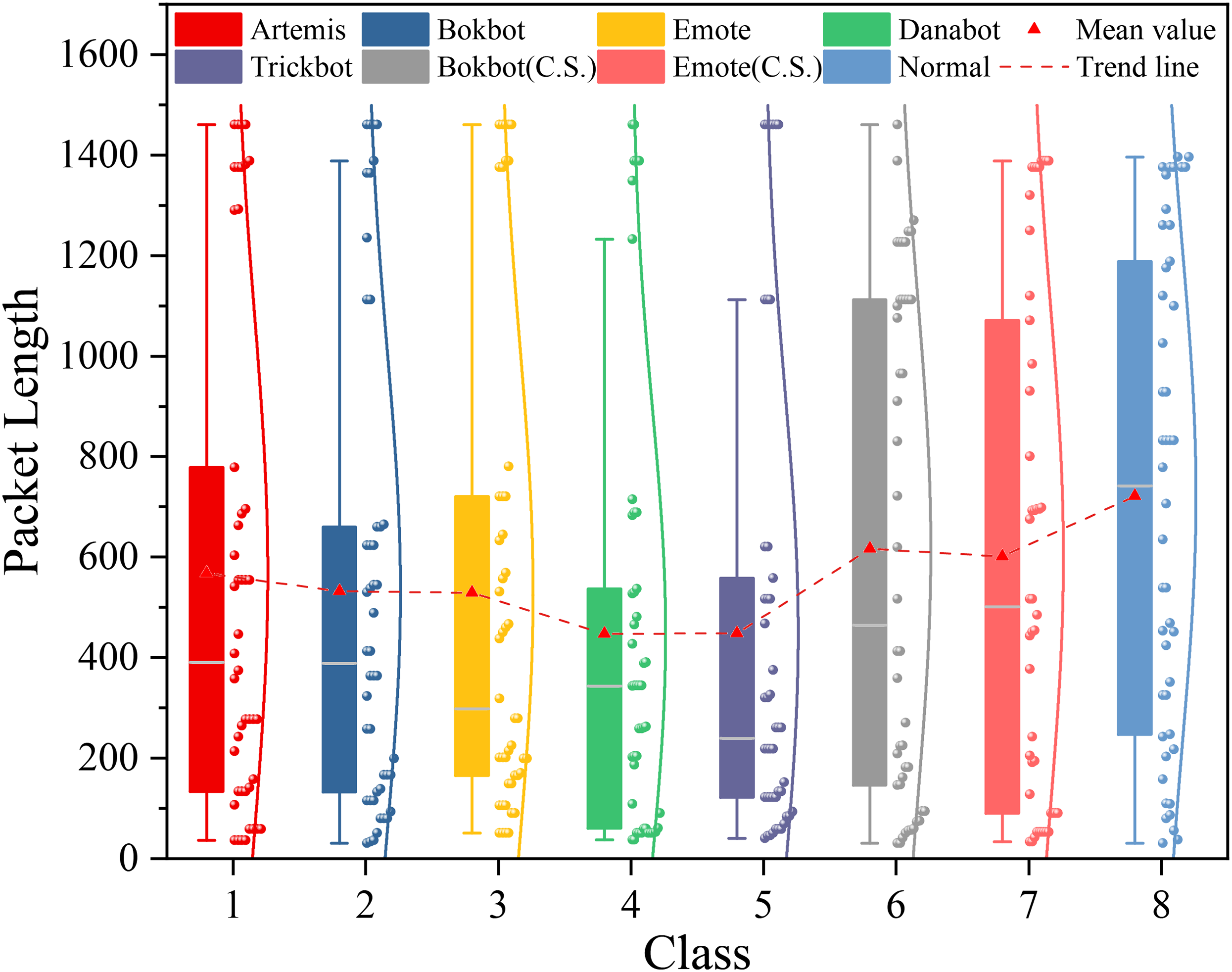
As discussed in the Related Work section, most network traffic analysis methods primarily rely on learning from time sequences of raw IP packets, such as their directed packet lengths and inter-arrival times (Sirinam et al., 2018; Liu et al., 2019). However, these temporal features can be distorted by both passive and active traffic obfuscation, causing their values to cluster around a limited set of discretized points. To investigate this effect, we analyze the MTA dataset and illustrate the packet length distributions of different categories in Fig. 3. For normal traffic, the packet length distribution is relatively uniform, spanning evenly from 0 to 1,500 bytes. In contrast, non-obfuscated malicious encrypted traffic, such as the Bokbot category, shows a more concentrated distribution. When obfuscation is applied, as in the Bokbot (C.S.) category, the distribution becomes similar to that of normal traffic, with the packet lengths concentrated around discretized values spread across the full 0 $\sim$ 1,500 range. As a result, directly inputting these distorted time-series features into a model may increase the likelihood of misclassification.

Figure 3: Distribution of packet lengths with confidence intervals in the MTA dataset among different types of malicious and normal traffic.

Download full-size image

DOI: 10.7717/peerj-cs.3353/fig-3

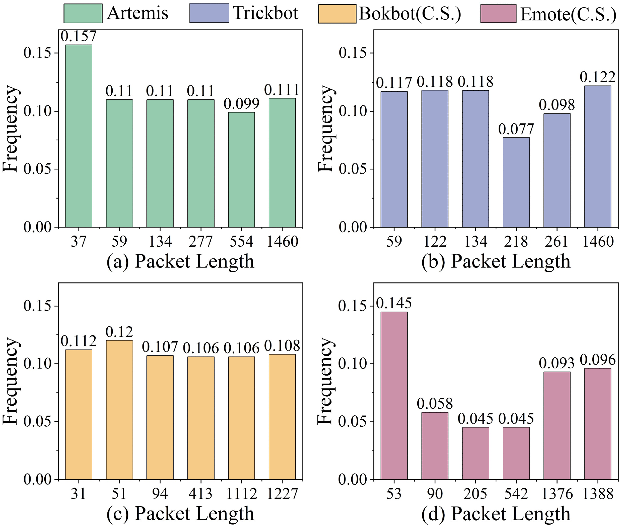
We further analyze the packet length frequency distributions across four malware categories in the MTA dataset. As shown in Fig. 4, different malware types exhibit distinct sets of high-frequency packet lengths. For instance, in Artemis, the 37-byte and 59-byte packet lengths each occur with frequencies exceeding 0.1, whereas in Bokbot (C.S.) under obfuscation, the 31-byte and 51-byte lengths are dominant. However, when traffic is subject to environmental noise and obfuscation, the overall distribution becomes more uniform, and the frequencies of individual packet lengths tend to decrease. This highlights the importance of standardizing packet-level features, such as packet length and inter-arrival time as shown in Fig. 2A2, to enhance the model’s ability to capture discriminative high-frequency patterns while mitigating the impact of low-frequency noise.

Packet lengths with the top-
${ k}$k
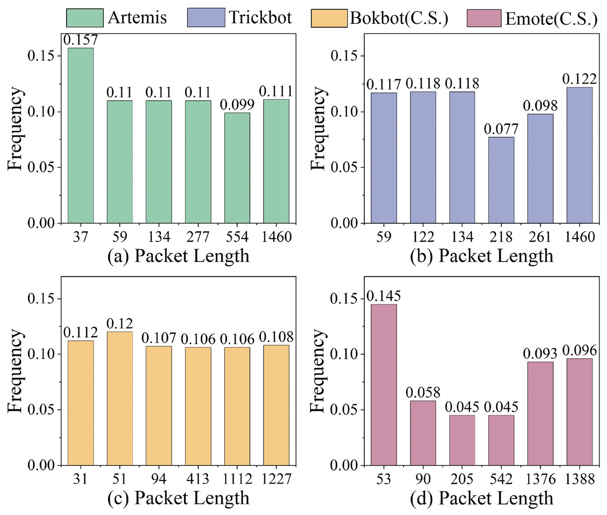
highest relative frequencies in MTA dataset for (A) Artemis, (B) Trickbot, (C) Bokbot (C.S.) and (D) Emote (C.S.) malware. — Figure 4: Packet lengths with the top- $k$ highest relative frequencies in MTA dataset for (A) Artemis, (B) Trickbot, (C) Bokbot (C.S.) and (D) Emote (C.S.) malware.

Download full-size image

DOI: 10.7717/peerj-cs.3353/fig-4

Traditional standardization methods tend to focus primarily on top- $k$ high-frequency values, which can result in the loss of semantically meaningful low-frequency variations (Liu et al., 2018; Li et al., 2023). To overcome this limitation, we propose an improved version of the Power Law Division (PLD) algorithm that adopts a hybrid discretization strategy. Specifically, the enhanced PLD defines a set of standardized packet lengths by combining (1) the top- $k$ most frequent packet lengths in the dataset, which preserves dominant traffic characteristics, and (2) regularly spaced values (e.g., every seven bytes), which ensure better coverage of rare but potentially informative patterns. This design not only addresses the bias of traditional methods toward high-frequency bins but also introduces a more balanced and robust standardization scheme that is resilient to obfuscation-induced noise. In contrast to existing PLD or quantization techniques that rely solely on frequency or uniform binning, our enhancement enables the model to more effectively capture both global and subtle structural variations in encrypted traffic.

Let $f$ be an encrypted network traffic flow identified by a five-tuple $⟨ c l i e n t I P$ , $s e r v e r I P$ , $c l i e n t P o r t$ , $s e r v e r P o r t$ , $P r o t o c o l ⟩$ . By monitoring a network interface, we can collect a sequence of IP packets belonging to flow $f$ , ordered by their timestamps: $f = {[p_{i}]}_{i = 1}^{T} = [p_{1}, p_{2}, \dots, p_{T}]$ , where $p_{i}$ denotes the $i$ -th packet in the flow and T is the total number of packets in $f$ . To extract packet-level features, we apply a function $P k t L e n (\cdot)$ to each packet in the sequence. The resulting time sequence of IP packet features is

(1) $P k t L e n (f) = [P k t L e n (p_{1}), \dots, P k t L e n (p_{T})],$ where $P k t L e n (p_{i})$ is a function to extract packet-level features from $p_{i}$ , such as the directed packet length, which is assigned a positive value if the packet is sent from client to server, and a negative value otherwise.

To standardize packet length sequences, we first analyze each traffic category $x$ to extract the top- $k$ most frequent packet lengths. These frequent lengths form the basis of a standardization function applied to each packet length sequence $P k t L e n (f)$ . Specifically, for each traffic category $x$ , we compute the frequency of all observed packet lengths and construct a ranked list $L^{x}$ , sorted in descending order of frequency. Each entry in $L^{x}$ is a pair $(ℓ_{j}^{x}, v_{j}^{x})$ , where $ℓ_{j}^{x}$ is the $j$ th most frequent packet length and $v_{j}^{x}$ is its corresponding frequency count. Formally, the frequency distribution is defined as:

(2) $L^{x} = [(ℓ_{j}^{x}, v_{j}^{x})] |_{j = 1}^{n^{x}},$ where $n^{x}$ is the total number of distinct packet lengths observed in category $x$ , and the list $L^{x}$ is sorted in descending order of frequency, such that $v_{j}^{x} \geq v_{j + 1}^{x}$ , for each $j \in [1, n^{x} - 1]$ . Considering both client-to-server and server-to-client directions, the number of distinct packet lengths can be as high as 1,500 $\times$ 2. To focus on the most representative values, we retain only the top- $k$ entries, resulting in a truncated list.

(3) $\tilde{L^{x}} = [(ℓ_{j}^{x}, v_{j}^{x})] |_{j = 1}^{k} .$

After obtaining the top- $k$ high-frequency packet length list $\tilde{L^{x}}$ for each traffic category $x$ , we define a function to measure the distance between any packet length and its closest match in $\tilde{L^{x}}$ . This distance is used to standardize packet lengths not present in the top- $k$ list. Specifically, for each packet $p_{i}$ in flow $f$ , we extract its length using $P k t L e n (p_{i})$ , and compute its distance to the closest value in the list $\tilde{L^{x}}$ :

(4) $d i s t (p_{i}, \tilde{L^{x}}) = min_{ℓ_{j}^{x} \in \tilde{L^{x}}} | P k t L e n (p_{i}) - ℓ_{j}^{x} | .$

For each packet $p_{i}$ in the flow $f$ , we apply a standardization function $S t d P k t L e n_{x} (p_{i})$ to its packet length:

(5) $S t d P k t L e n^{x} (p_{i}) = {\begin{matrix} \underset{ℓ_{j}^{x} \in \tilde{L^{x}}}{\arg min} | P k t L e n (p_{i}) - ℓ_{j}^{x} |, & i f d i s t (p_{i}, \tilde{L^{x}}) \leq Δ τ, \\ ⌈ \frac{P k t L e n (p_{i})}{Δ τ^{'}} ⌉ \times Δ τ^{'}, & o t h e r w i s e . \end{matrix}$

Equation (5) defines a packet length standardization function. It first extracts the packet length by $P k t L e n (p_{i})$ and calculates its closest distance $d i s t (p_{i}, \tilde{L^{x}})$ to the top- $k$ frequent packet lengths in the list $\tilde{L^{x}}$ . If the distance is within a threshold $Δ τ$ , the packet length is replaced with the nearest top- $k$ frequent value; otherwise, it is rounded to the nearest multiple of $Δ τ^{'}$ , which is set to 7 by default. By this standardization process, the time series noise interference caused by traffic obfuscation can be effectively mitigated, thus enhancing the model’s ability to learn the high-frequency features of malicious activities.

As shown in Eq. (5), $Δ τ^{'}$ is a hyperparameter that controls the granularity of standardizing non-high-frequency packet lengths. We set $Δ τ^{'} = 7$ by default, striking a practical balance between reducing obfuscation-induced noise and retaining meaningful variation. This choice was empirically found to yield stable performance across multiple datasets. We acknowledge that the model’s sensitivity to $Δ τ^{'}$ is an important factor affecting its robustness to different obfuscation strategies, and we will analyze this in detail in the Experiments section of the revised manuscript.

Design and construction of adaptive sliding window Flow-level burst graph

In this section, we present the algorithm design for constructing the AFG. First, we propose an adaptive sliding window algorithm to capture dynamic behaviors in network traffic. Based on this algorithm, we construct a flow-level burst graph to effectively identify malicious traffic patterns. Finally, we discuss the advantages of AFG compared to the fixed time windows and other flow relation graph construction methods (Jiang et al., 2022; Yang et al., 2024a).

Grouping flows into session windows by adaptive sliding window algorithm

Malware often generates substantial network traffic during its execution, and due to variations in attack tools and techniques, this traffic exhibits diverse behavioral patterns, for example, sudden surges during DDoS attacks, periodic fluctuations in command-and-control (C&C) communications or crypto-mining, and repeated requests in web crawling (Jiang et al., 2022). To better capture these behaviors, we group five-tuple flows that share the same client and server IP addresses into broader two-tuple session windows. Compared to individual five-tuple flows, these session windows span longer durations and offer a more comprehensive view of client-server interactions. Within each session window, multiple flows are organized into a flow-level relation graph, facilitating the detection of malicious encrypted traffic.

To construct these flow graphs more effectively, we propose an adaptive sliding window algorithm. The intuition behind this heuristic is that malicious flows tend to occur in concentrated bursts. Fixed-size windows may fragment these bursts or inadvertently include unrelated flows, thereby disrupting the temporal coherence of flow sequences. Our adaptive sliding window addresses this by dynamically adjusting its size based on the average inter-flow time within the current window. This average acts as a data-driven threshold to determine whether subsequent flows should be incorporated, allowing the window to adapt to local traffic density and better preserve temporal consistency. We also acknowledge the potential limitations of this approach. In highly bursty or irregular traffic, the average inter-arrival time may serve as an unstable or non-discriminative threshold. In future work, we plan to explore alternative strategies, such as using median-based or percentile-based thresholds, to improve robustness.

In contrast, prior methods for building flow-level relation graphs use fixed-size time windows (Jiang et al., 2022; Yang et al., 2024a), which are inadequate for capturing dynamic traffic behaviors. These static approaches may miss burst events or extended anomalies that fall outside the rigid window boundaries, leading to reduced detection accuracy. Our adaptive strategy mitigates this issue by flexibly capturing temporal variations and preserving interaction information critical for identifying malicious behavior.

The pseudocode is presented in Algorithm 1, whose detailed steps are explained below. First, Line 1 inserts the input traffic flow $f_{i}$ to the sliding window $W_{t}$ within a same two-tuple session window, if $W_{t}$ is now empty. The set of flows contained in the current sliding window $W_{t}$ is defined as:

(6) $W_{t} = {f_{i} ∣ t_{i} < t_{1} + T_{i n i t} \lor (t_{i} \leq t_{i - 1} + {\bar{Δ t}}_{1, | W_{t} |} \land t_{i} \leq t_{1} + T_{m a x})},$ where $t_{i}$ is the start timestamp of the $i$ -th flow $f_{i}$ , $T_{i n i t}$ is the initial size of the sliding window, and $T_{m a x}$ is the maximum allowable size of the sliding window. For each flow $f_{i}$ , in Line 3, we calculate the time interval $Δ T_{i}$ between $f_{i}$ and the first flow $W_{t} [1]$ in the sliding window. If the interval $Δ T_{i}$ is smaller than the threshold $T_{i n i t}$ , then the flow is appended to the sliding window $W_{t}$ in Line 4. Otherwise, the time interval $Δ t_{i}$ between $f_{i}$ and the last flow in $W_{t}$ is calculated, followed by computing the average time interval ${\bar{Δ t}}_{1, | W_{t} |}$ across all intervals in Line 6 and as Eq. (7):

(7) ${\bar{Δ t}}_{1, | W_{t} |} = \frac{1}{| W_{t} | - 1} \sum_{i = 2}^{| W_{t} |} Δ t_{i}, w i t h Δ t_{i} = t_{i} - t_{i - 1},$ where $| W_{t} |$ is the number of flows in the current sliding window, and $Δ t_{i}$ is the time interval between the $i$ -th flow and its previous flow. The average time interval ${\bar{Δ t}}_{1, | W_{t} |}$ serves as a threshold to determine whether a new flow $f_{i}$ can be appended to the sliding window. This criterion ensures that $f_{i}$ is temporally close to the preceding flows, suggesting that it is part of the same bursty behavior. Additionally, it guarantees that the inclusion of $f_{i}$ reduces the average time interval within the the session window, reinforcing its temporal cohesion. Next, we compute the time interval between the new flow $f_{i}$ and the last flow in the current window as $Δ t_{i} = t_{i} - t_{i - 1}$ in Line 7. If $Δ t_{i} \leq {\bar{Δ t}}_{1, | W_{t} |}$ and the time interval of the window $Δ T_{i} = t_{i} - t_{1}$ does not exceed the preset maximum window size $T_{m a x}$ , the window slides in Line 8. Otherwise, the algorithm return NIL in Line 9, indicating the current window $W_{t}$ has ended and a new window should begin.

Algorithm 1 :

InsertFlow2AdaptiveSlidingWindow algorithm.

Input: f_i: A network flow to be inserted, W_t: Adpative sliding window containing concurrent flows between a pair of client and server IPs, and sorted by timestamps, T_init: Initial window size, T_max: Maximum allowable window size

Output: W_t: Updated adpative sliding window if flow f_i is successfully inserted, otherwise NIL

1 if sliding window W_t is an empty set ϕ then append the new flow f_i to the end of W_t

2 else

Δ T_{i}

f_{i} . t s - W_{t} [1] . t s

// Compute time interval between first flow and flow f_i

4 if

Δ T_{i} \leq T_{i n i t}

then append the new flow f_i to the end of W_t

5 else

6 calculate average inter-flow time

{\bar{Δ t}}_{1, | W_{t} |}

in W_t

Δ t_{i}

f_{i} . t s - W_{t} [- 1] . t s

// Compute time interval between last flow and flow f_i

// Sliding window if

Δ t_{i} \leq {\bar{Δ t}}_{1, | W_{t} |}

(average interval) and

Δ T_{i}

within max size

8 if

Δ t_{i} \leq {\bar{Δ t}}_{1, | W_{t} |}

and

Δ T_{i} \leq T_{m a x}

then append the new flow f_i to the end of W_t

9 else return NIL // Insertion fails, and please start a new sliding window

10 return W_t

DOI: 10.7717/peerj-cs.3353/table-101

An example is illustrated in the bottom part of Fig. 2B1. The flows $f_{1}$ , $f_{2}$ , and $f_{3}$ are directly loaded as their cumulative time span $t_{3} - t_{1}$ is smaller than the initial window size $T_{i n i t}$ . Subsequently, the flows $f_{4}$ through $f_{8}$ are appended one by one, as the time intervals between each new flow and its preceding flow ( $Δ t_{i} = t_{i} - t_{i - 1}$ ) is smaller than the current average interval within the window ( ${\bar{Δ t}}_{1, | W_{t} |}$ ). This results in a non-increasing trend in the average interval, i.e., ${\bar{Δ t}}_{1, 3} \geq {\bar{Δ t}}_{1, 4} \geq \dots \geq {\bar{Δ t}}_{1, 8}$ , after appending flows $f_{3}, f_{4}, \dots, f_{8}$ . As ${\bar{Δ t}}_{1, 9} > {\bar{Δ t}}_{1, 8}$ , the inclusion condition is no longer satisfied, and flows $f_{1}$ to $f_{8}$ are thus grouped into a single session window. Through this algorithm, we can more accurately reveal the behavioral patterns of malicious encrypted traffic and improve the model’s representational capability.

From a theoretical perspective, this adaptive sliding window algorithm operates in a single pass over all captured flows sorted by their start timestamps. Since no backtracking, sorting, or pairwise comparison is involved, this algorithm only computes a dynamic threshold to determine window boundaries based on local burst characteristics. So, its time cost is $O (n)$ with respect to the number of flows $n$ observed in the traffic and inserted by this algorithm. This design ensures high efficiency on large-scale traffic datasets.

Construction of flow-level burst graph for each session window

As mentioned previously, malware often generates multiple network flows during attack activities, with some flows occurring concurrently within a short time window to fulfill a coordinated purpose, thereby forming one or more bursts (Oudah et al., 2019). Recent studies have shown that such multi-flow burst behavior is crucial for analyzing encrypted traffic (Jiang et al., 2022; Zhu et al., 2023). Constructing a flow relation graph that captures multiple bursts is essential for uncovering complex interactions between client and server hosts. In this graph, both the number of concurrent flows within each burst and the frequency of bursts are closely linked to underlying attack patterns. Constructing inter-flow relationships in this way enhances model’s representational capability and helps mitigate the impact of traffic obfuscation.

As inspired by FG-Net (Jiang et al., 2022), our flow-level burst graph is designed to capture both concurrent and trigger relationships among five-tuple flows within a session window, which shares a common pair of client and server IPs and have proximate flow start times. In this graph, flows within the same burst are considered to share a concurrent relationship, while the bursts, ordered by their starting timestamps, are linked through trigger relationships between adjacent pairs. This trigger information is closely tied to the behavioral patterns of malicious encrypted traffic. Unlike traditional flow-level relationship graph, our flow-level burst graph is built based on the adaptive sliding window algorithm, which dynamically adjusts the window size to better capture bursts behaviors.

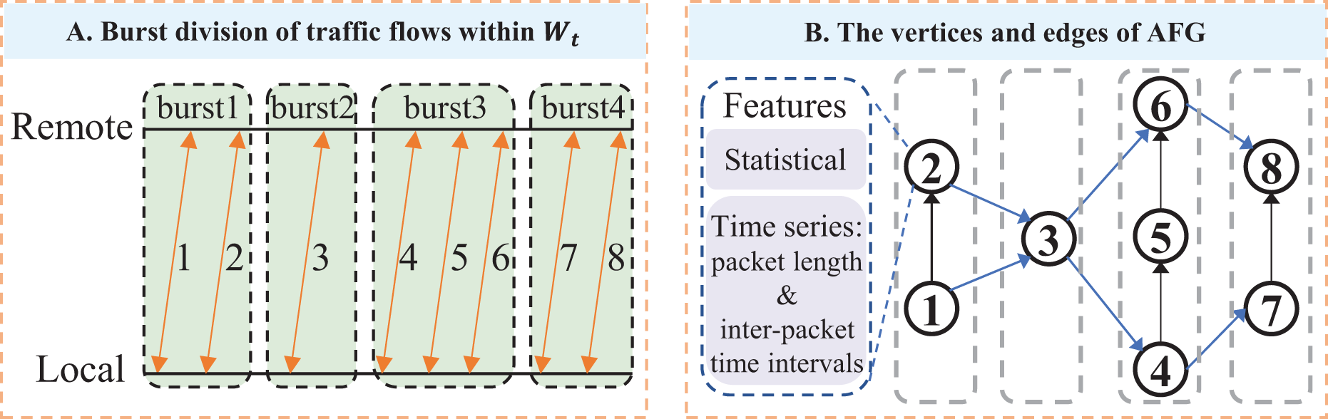
An example of AFG: An example of the AFG is illustrated in Fig. 5A. Eight flows are collected from the adaptive sliding window $W_{t}$ : flows 1 and 2 belong to burst 1, flow 3 to burst 2, flows 4, 5, and 6 to burst 3, and flows 7 and 8 to burst 4. In the corresponding AFG shown in Fig. 5B, each vertex represents a traffic flow and is characterized by statistical and time-series features. For concurrent relationships, vertex 1 connects to vertex 2 within burst 1, and vertices 4, 5, and 6 are connected sequentially within burst 3, indicating intra-burst concurrency. For trigger relationships, vertices 1 and 2 connect to vertex 3, reflecting the trigger relationship from burst 1 to burst 2. Similarly, vertices 4 and 6 connect to vertices 7 and 8, indicating the trigger relationship between bursts 3 and 4.

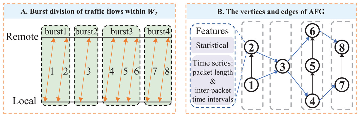
Construct Adaptive sliding-window Flow-level burst Graph (AFG) for a client-server IP pair: (A) For a client-server IP pair, observe their transmitted five-tuple flows within
${{ W}_{ t}}$Wt
time window, and group the concurrent flows with proximate start times into bursts; (B) For an AFG, vertices are flows with statistical features and directed packet length sequence features, while edges denote concurrent and trigger relationships between flows. — Figure 5: Construct Adaptive sliding-window Flow-level burst Graph (AFG) for a client-server IP pair: (A) For a client-server IP pair, observe their transmitted five-tuple flows within $W_{t}$ time window, and group the concurrent flows with proximate start times into bursts; (B) For an AFG, vertices are flows with statistical features and directed packet length sequence features, while edges denote concurrent and trigger relationships between flows.

Download full-size image

DOI: 10.7717/peerj-cs.3353/fig-5

We present the pseudocode in Algorithm 2 for constructing the flow-level burst graph. We first collect all traffic flows generated between a client-server pair and arrange them in ascending order based on their start timestamps, forming the sequence $F = {f_{1}, f_{2}, \dots f_{i} \dots}$ . For all flows $f_{i} \in F$ , we process them by the adaptive sliding window, splitting them into bursts and constructing an AFG. This graph consider both the concurrent relationship among flows within a same burst and the trigger relationship between bursts.

Partition a client-server session into session windows: The construction of the current session window $W_{t}$ terminates when the input flow $f_{i}$ is NIL, or when the function InsertFlow2AdaptiveSlidingWindow() returns NIL in Line 11, which subsequently triggers the start of the next session window. For each completed session window, we construct an AFG in Lines 6 to 16, which contains two type of edges for concurrent and trigger relationships, respectively.
Concurrent relationship: Assume $W_{t} = {f_{1}, f_{2}, \dots, f_{n}}$ is a session window of five-tuple flows collected between a pair of client and server hosts and ordered by their starting timestamps. We partition them into bursts according to the proximaty of these flows’ start times. If the time interval between a pair of adjacent flows $Δ t_{i}$ is less than the pre-configured threshold $δ$ , these two flows are considered concurrent and are grouped into the same burst by Lines 6 to 11.
Trigger relationship: The termination of the current burst ${f_{1}, f_{2}, \dots, f_{k}}$ is detected, when the time interval between $f_{k}$ and $f_{k + 1}$ exceeds the threshold $δ$ , which subsequently triggers the initiation of the next burst ${f_{k + 1}, f_{k + 2}, \dots, f_{k + j}}$ in Line 14. A trigger relationship is then established between these two time-adjacent bursts by invoking the InsertEdges() function in Line 13. This relationship is encoded using two directed edges, as shown in Lines 18 to 20: one from the first flow of the previous burst to the first flow of the next burst, and another from the last flow of the previous burst to the last flow of the next burst, which have been illustrated in Fig. 5B.

Algorithm 2 :

InsertFlow2AFG: adaptive flow-level burst graph for client-server session window.

Input: f_i: A network flow to be inserted within a same pair of client and server IPs, W_t: Adpative sliding window containing concurrent flows between a pair of client and server IPs, and sorted by timestamps, T_init: Initial window size, T_max: Maximum allowable window size

Output:

G = (V, E)

: Flow-level burst graph for a completed client-server session window W_t

1 if

f_{i} \neq N I L \land

InsertFlow2AdaptiveSlidingWindow

(f_{i}, W_{t}, T_{i n i t}, T_{m a x}) \neq N I L t h e n

// Algorithm 1

2 return NIL //Insertion success, and the session window grows continuously

3 Assume

W_{t} = {f_{1}, f_{2}, \dots, f_{n}}

is a session window of five-tuple flows collected between a pair of client and server hosts and ordered by their starting timestamps

V = \emptyset, E = \emptyset

// Initialize vertex and edge sets

5 curr_burst

= \emptyset,

last_burst

= \emptyset

// Initialize curr_burst and last_burst

6 for each flow $f_{i} \in W_{t}$ do

7 V.insert(f_i) // Add flow f_i to the vertex set V of flow relation graph G

8 if

c u r r_b u r s t == \emptyset

then

c u r r_b u r s t = [f_{i}]

// Init curr_burst as a flow list with only f_i

9 else

10 if

(Δ t_{i} = f_{i} . t s - c u r r_b u r s t [- 1] . t s) \leq δ

then

11 append the new flow f_i to the end of curr_burst

12 else

13 call InsertEdges (

E, l a s t_b u r s t, c u r r_b u r s t

)

// Save curr_burst to last_burst, and start a new curr_burst with empty set

l a s t_b u r s t = c u r r_b u r s t, c u r r_b u r s t = \emptyset

15 if

c u r r_b u r s t \neq \emptyset

then call InsertEdges (

E, l a s t_b u r s t, c u r r_b u r s t

) // Handle last burst

16 return

G = (V, E)

17 Function InsertEdges (

E, l a s t_b u r s t, c u r r_b u r s t

)

18 if

l a s t_b u r s t \neq \emptyset

then

// Add a trigger edge between the first flows of last_burst and curr_burst

19 E.insert(last_burst

[1]

, curr_burst

[1]

)

// Add a trigger edge between the last flows of last_burst and curr_burst

20 E.insert(last_burst

[- 1]

, curr_burst

[- 1]

)

// Add concurrent edges between each pair of adjacent flows in curr_burst

21 for

i = 2, \dots, | c u r r_b u r s t |

do E.insert(curr_burst

[i - 1]

, curr_burst[i])

DOI: 10.7717/peerj-cs.3353/table-102

Additionally, this flow-level burst graph construction algorithm processes flows sequentially within each session window. It performs constant-time operations for vertex insertion and edge creation without requiring backtracking or global sorting. Thus, its time cost is $O (n)$ with respect to the number of flows $n$ in the session window. This ensures efficient graph construction even under large-scale traffic datasets.

Summarizing advantages of AFG

AFG offers a more precise and comprehensive approach to detecting malicious encrypted traffic by dynamically adjusting time windows, thereby capturing bursts and anomalous behavior in network traffic. Compared to traditional flow relation graphs, AFG has several notable advantages:

Time window size adjustment ability:Traditional flow relation graphs rely on fixed time windows (Jiang et al., 2022; Yang et al., 2024a), which struggle to handle dynamic changes in traffic. While AFG employs an adaptive sliding window algorithm to automatically adjust the window size based on traffic fluctuations, enabling a more flexible capture of dynamic behavior in network flows. This addresses the issue of missing interaction topology information when using fixed time windows.
Rich intra-flow features: In AFG, each traffic flow contains rich multi-granularity features, such as per-flow statistical features, temporal packet length sequences, and inter-packet arrival time sequences. These features are preserved through the vertices of the graph, enabling the flow-level burst graph not only to capture the inter-flow relations but also to delve into the detailed characteristics of each flow.
Enhanced inter-flow relational information: Malicious encrypted traffic often exhibits bursty patterns and trigger relationships. AFG enhances flow-level modeling using directed edges to represent concurrent and trigger relations between traffic flows. Through the adaptive sliding window mechanism, AFG explicitly captures these relationships, allowing them reflect the actual traffic patterns more accurately.

Fusing spatial-temporal features in AFG by CNN, transformer and GNN hybrid models

After standardizing the intra-flow time series features and constructing the AFGs to capture inter-flow relational information, we need to extract and fuse the spatial-temporal features in AFGs. For each flow, we use CNN to encode temporal statistical features, and employ the BERT model to capture long-range dependencies in its IP packet sequence (Lin et al., 2022). The encoded flow-level features are incorporated as vertex attributes, and then propagated and fused within the spatial topology of the AFG through GAN. This spatial-temporal feature fusion model leverages the complementary advantages of different features, thereby enhancing the model’s representational capability and predictive accuracy. The notations used in this section are summarized in Table 2.

Table 2:

Summarization of notations used in the model architecture and typical hyperparameter settings.

Component	Operation/Layer	Symbol	Shape/Dimension
CNN feature extractor in subsec. Intra-flow statistical features modeling	Input statistical vector	$x_{f}, x_{f}^{(1)}$	$R^{d_{f}}$ with $d_{f} = 103$
	Conv1D layer 1 weights	$W_{f}^{(1)} / b_{f}^{(1)}$	$R^{32 \times 1 \times 8} / R^{32}$
	Conv1D + BN + ReLU	$h_{f}^{(1)}$	$R^{103 \times 32}$
	Conv1D layer 2 weights	$W_{f}^{(2)} / b_{f}^{(2)}$	$R^{32 \times 32 \times 8} / R^{32}$
	Conv1D + BN + ReLU	$h_{f}^{(2)}$	$R^{103 \times 32}$
	MaxPooling1D	$h_{f}^{(3)}$	$R^{11 \times 32}$
	Flatten	$F l a t t e n (h_{f}^{(3)})$	$R^{1 \times 352}$
	Fully connected weights	$W_{f}^{(3)} / b_{f}^{(3)}$	$R^{256 \times 352} / R^{256}$
	Tanh + BN	$z_{f}$	$R^{1 \times 256}$
BERT encoder in subsec. Intra-flow IP packet sequence features modeling	Input length/time sequence	$X_{s}, X_{a}$	$R^{1 \times m}$ with $m = 25$
	Embedding projection weight	$W_{s}, W_{a}$	$R^{256 \times 1}$
	Embedding projection bias	$b_{s}, b_{a}$	$R^{256}$
	Projected embedding	$H_{s}^{(1)}, H_{a}^{(1)}$	$R^{256 \times 25}$
	BERT input	${X_{s}}^{'}, {X_{a}}^{'}$	$R^{1 \times 25 \times 256}$
	Transformer layers	L	4
	Hidden size	$d$	256
	Attention heads/head dim	$h / d_{k}$	4/64
	Query/Key/Value vector	$Q^{(l)}, K^{(l)}, V^{(l)}$	$R^{25 \times 64}$
	Q/K/V projection weights	$W_{Q}^{(l)}, W_{K}^{(l)}, W_{V}^{(l)}$	$R^{256 \times 64}$
	Output projection weight	$W_{O}^{(l)}$	$R^{256 \times 256}$
	Layer output	$H_{s}^{(l)}, H_{a}^{(l)}$	$R^{25 \times 256}$
	CLS output vector	$z_{s}, z_{a}$	$R^{256}$
Graph attention network in subsec. Inter-flow relational feature modelling	Input features (stat/pktlen/iat)	$z_{f}, z_{s}, z_{a}$	$R^{256}$
	GATConv Layer 1/2 output	$h_{i}^{(1)} / h_{i}^{(2)}$	$R^{512} / R^{256}$
	Attention heads	K	2 (1st), 1 (2nd)
	Attention weight vector (head $k$ )	$a^{(1)} [k] / a^{(2)} [k]$	$R^{256} / R^{512}$
	Linear transform weight (head $k$ )	$W_{r}^{(1)} [k] / W_{r}^{(2)} [k]$	$R^{256 \times 256} / R^{512 \times 256}$
	Output node embeddings	$H_{f}, H_{s}, H_{a}$	$R^{N \times 256}$
	Global feature (mean pooling)	$H_{g l o b a l}$	$R^{1 \times 768}$
	Fusion weight matrix/bias	$W_{o}$ / $b_{o}$	$R^{256 \times 768} / R^{256}$
	Final GAT output feature	$z_{g l o b a l}$	$R^{256}$
Linear classifier in subsec. Client-server session window classification	Input feature vector	$z_{g l o b a l}$	$R^{256}$
	Classification weight/bias	$W_{c} / b_{c}$	$R^{C \times 256} / R^{C}$
	Output probabilities	$\hat{y}$	$R^{C}$
	Ground-truth one-hot label	$y$	$R^{C}$
	Loss function	$L_{C E}$	Cross-entropy

DOI: 10.7717/peerj-cs.3353/table-2

Intra-flow statistical features modeling

For each flow, we extract its statistical feature vector, resulting in a total of $d_{f} = 103$ statistical features. To project them into lower-dimensional embeddings, we apply convolutional neural networks (CNNs), which enhance feature expressiveness by capturing local patterns and inter-feature relationships through convolution operations. Prior studies have shown that incorporating CNNs to process temporal statistical features can significantly improve model performance (Hnamte & Hussain, 2023; Mo et al., 2024).

Before constructing the feature extraction model, We first normalize the temporal statistical feature vector $X_{f} \in R^{d_{f}}$ to ensure compatibility with the input format of the neural network, as shown in Eq. (8).

(8) $x_{f}^{(1)} = (x_{f} - μ_{f}) / σ_{f},$ where $x_{f}^{(1)}$ is the normalized feature vector, $μ_{f}$ and $σ_{f}$ are the mean and standard deviation of the feature vector, respectively. The normalized feature vector is then input into CNN for modeling.

As shown in Fig. 2C2, the embedding model has three layers. The first layer is a convolutional layer, where we apply filters to perform convolution operations on the input features $x_{f}^{(1)}$ , expressed as follows:

(9) $h_{f}^{(1)} = R e L U (B N (C o n v 1 D (x_{f}^{(1)}, W_{f}^{(1)}) + b_{f}^{(1)})),$ where $C o n v 1 D (x_{f}^{(1)}, W_{f}^{(1)})$ is the convolution operation, $W_{f}^{(1)}$ is the weight matrix of the first convolutional layer, $b_{f}^{(1)}$ is the bias term, and $B N$ is batch normalization. The convolution operation extracts local feature patterns, with the $R e L U$ activation function enhancing non-linear capacity.

The second layer repeats the above process but employs a second convolutional filter with the same kernel sizes but different parameters $W_{f}^{(2)}$ and $b_{f}^{(2)}$ to extract higher-level features $h_{f}^{(2)}$ . This is followed by a downsampling pooling layer, to reduce feature dimensionality and improve computational efficiency.

(10) $h_{f}^{(3)} = M a x P o o l i n g 1 D (h_{f}^{(2)}) .$

After two layers of convolution and pooling, the final feature map $h_{f}^{(3)}$ is flattened and mapped to the target dimension through a fully connected layer, as expressed in Eq. (11),

(11) $z_{f} = T a n h (B N (W_{f}^{(3)} F l a t t e n (h_{f}^{(3)}) + b_{f}^{(3)})),$ where $F l a t t e n ()$ is a function for reshaping the input tensor into a one-dimensional vector $h_{f}^{(2)}$ by concatenating all elements in a fixed order, $W_{f}^{(3)}$ and $b_{f}^{(3)}$ denote the weight matrix and bias vector of the fully connected layer, respectively, $B N$ is batch normalization operation, $T a n h ()$ is the hyperbolic tangent activation function, and $z_{f}$ is a representation of the statistical features of the given five-tuple flow. Later, $z_{f}$ is also treated as the vertex feature of an AFG containing this flow.

Intra-flow IP packet sequence features modeling

In addition to temporal statistical features, the time series features, such as packet length and inter-packet arrival times, are also valuable for classifying malicious encrypted traffic. To model the time series features, we use the BERT model due to its self-attention mechanism, which effectively captures long-range dependencies and complex temporal patterns in packet-level time series data. This mechanism has been proven in prior work like ET-BERT (Lin et al., 2022) to enhance the detection of encrypted traffic.

Before modeling the time series features, the packet length sequence needs to be standardized by the improved PLD algorithm. Since Transformer-based models are good at word embedding for textual data (Koroteev, 2021), we need to map the raw numerical features (e.g., packet length sequences) into a high-dimensional embedding space $h_{i}$ through a fully connected layer (Yang et al., 2024b). As shown in Fig. 2C1, for the packet length example, $L = {L_{1}, L_{2}, \dots, L_{m}}$ , where $m$ represents the sequence length, its mapping process can be expressed as Eq. (12). Let $d$ be the dimension of the high-dimensional embedding space, $X_{s}$ be the matrix $\in R^{1 \times m}$ for the packet-length feature vector counted in bytes, $X_{a}$ be the matrix $\in R^{1 \times m}$ for the inter-arrival time features for each of the $m$ packets. Then,

(12) $H_{s}^{(1)} = R e L U (W_{s} X_{s} + b_{s} \otimes 1_{m}^{⊤}), H_{a}^{(1)} = R e L U (W_{a} X_{a} + b_{a} \otimes 1_{m}^{⊤}),$ where $W_{s}, W_{a} \in R^{d \times 1}$ are the weight matrices that project each scalar input into a $d$ -dimensional embedding space; $b_{s}, b_{a} \in R^{d}$ are the bias vectors; $1_{m} \in R^{m}$ is an all-ones vector used to broadcast the bias across the sequence dimension; $\otimes$ denotes the outer product. $H_{s}^{(1)}, H_{a}^{(1)} \in R^{d \times m}$ are the resulting high-dimensional embeddings for each packet’s length and inter-arrival time, respectively, where each column corresponds to one packet.

To process the packet length embedding sequence $H_{l}^{(1)}$ , we use it as the input sequence of the BERT model. This model captures long-range dependencies within the time series through its multi-head self-attention mechanism (Koroteev, 2021). Its computational process is as follows:

(13) $\begin{matrix} Q^{(l)} = H_{s}^{(l - 1)} W_{Q}^{(l)}, K^{(l)} = H_{s}^{(l - 1)} W_{K}^{(l)}, V^{(l)} = H_{s}^{(l - 1)} W_{V}^{(l)}, \\ A t t e n t i o n^{(l)} (H_{s}^{(l - 1)}) = S o f t m a x (Q^{(l)} {(K^{(l)})}^{⊤} / \sqrt{d_{k}}) V^{(l)}, \\ H_{s}^{(l)} = L a y e r N o r m (A t t e n t i o n^{(l)} (H_{s}^{(l - 1)}) + H_{s}^{(l - 1)}), \end{matrix}$ where $W_{Q}^{(l)}, W_{K}^{(l)}, W_{V}^{(l)} \in R^{d \times d_{k}}$ are the weight matrices of the linear projections used to compute the queries, keys, and values at the $l$ -th Transformer layer; $d_{k}$ is the dimensionality of the query/key space, typically set to $d / h$ , where $h$ is the number of attention heads (for single-head attention, $d_{k} = d$ ); and $L a y e r N o r m (\cdot)$ is the layer normalization operation applied after the residual connection. This multi-layer BERT model outputs the representations of the $m$ tokens in the sequence $H_{s}^{(l)} = [h_{c l s}, h_{1}, h_{2}, \dots, h_{m}]$ along with a classification token $h_{c l s}$ in the front, which aggregates information of the entire sequence. The vector $h_{c l s}$ will be renamed as $z_{s}$ and used as the five-tuple flow’s IP packet length sequence representations:

(14) $z_{s} = H_{s}^{(l)} . h_{c l s}, z_{a} = H_{a}^{(l)} . h_{c l s} .$

To process the packet inter-arrival time embedding sequence $H_{a}^{(1)}$ , we use it as the input sequence of another BERT model. This model processes $H_{a}^{(1)}$ in the same way as Eq. (13), resulting in high-dimensional representations $H_{a}^{(l)}$ for the inter-arrival time sequence. From its output, we also extract the classification token as the vector $z_{a}$ , which is used for inter-arrival time sequence embeddings. Finally, for each five-tuple flow, we obtain three embedding vectors: $z_{f}$ , derived from the flow’s statistical features; $z_{s}$ , derived from its IP packet length sequence; and $z_{a}$ , derived from its inter-arrival time sequence.

Inter-flow relational feature modelling for each client-server session window

After modeling the statistical and time series features, TransGraphNet employs a Graph Attention Network (GAT) to capture inter-flow relational information within the AFG. By aggregating temporal features of the vertices in a spatial graph structure, GAT produces a global representation of the AFG, which is then used for the downstream session window classification task. The core idea of GAT is to dynamically assign attention weights to each vertex via a self-attention mechanism (Veličković et al., 2017), enabling the model to focus on the most relevant relationships and features within each vertex’s neighborhood.

For each vertex $v_{i}$ , GAT aggregates features by learning the importance weights $α_{i j}^{(l)}$ of its neighbor vertices $v_{j}$ . This process can be expressed by Eq. (15):

(15) $α_{i j}^{(l)} = {S o f t m a x}_{j} (L e a k y R e L U (⟨ a^{(l)}, [W_{r}^{(l)} h_{i}^{(l)} | | W_{r}^{(l)} h_{j}^{(l)}] ⟩)),$ where $h_{i}^{(l)}$ is the input feature of vertex $v_{i}$ at the $l$ -th GAT layer, $W_{r}^{(l)}$ is the learnable linear transformation matrix at layer $l$ , $a^{(l)}$ is the trainable vector used to compute attention scores, and ∥ is vector concatenation. The coefficient $α_{i j}^{(l)}$ denotes the normalized attention weight from neighbor vertex $v_{j}$ to $v_{i}$ at layer $l$ . The subscript $j$ in $S o f t m a x_{j}$ indicates that the softmax normalization is performed over all neighbor vertices $v_{j} \in N (i)$ , so that the attention weights $α_{i j}^{(l)}$ for a given vertex $v_{i}$ sum to 1. After applying the weights $α_{i j}^{(l)}$ , GAT generates a new feature representation $h_{i}^{(l + 1)}$ for each vertex as shown in Eq. (16):

(16) $h_{i}^{(l + 1)} = σ (\sum_{j \in N (i)} α_{i j}^{(l)} W_{r}^{(l)} h_{j}^{(l)}),$ where $σ$ is the activation function (e.g., $R e L U$ ), and $N (i)$ denotes the set of neighbor vertices for vertex $v_{i}$ .

To enhance the model’s expressiveness, GAT utilizes a multi-head attention mechanism, in which multiple attention heads operate in parallel (Veličković et al., 2017). The outputs of these heads are concatenated or averaged to generate the final vertex representation, as expressed in Eq. (17):

(17) $h_{i}^{(l + 1)} = \sum_{k = 1}^{K} σ (\sum_{j \in N (i)} α_{i j}^{(l)} [k] W_{r}^{(l)} [k] h_{j}^{(l)}),$ where $h_{i}^{(l)}$ is the input feature of vertex $v_{i}$ at the $l$ -th layer, $h_{i}^{(l + 1)}$ is the updated feature at the $(l + 1)$ -th layer, $N (i)$ is the set of neighbors of vertex $v_{i}$ , K is the number of attention heads, $α_{i j}^{(l)} [k]$ is the normalized attention coefficient from neighbor $v_{j}$ to $v_{i}$ computed by the $k$ -th head, $W_{r}^{(l)} [k]$ is the trainable weight matrix for the $k$ -th attention head at layer $l$ , and $σ (\cdot)$ is a non-linear activation function such as ReLU.

For spatiotemporal feature fusion, the per-flow statistical feature embeddings $z_{f}$ in Eq. (11), packet length sequence embeddings $z_{s}$ , and packet inter-arrival time embeddings $z_{a}$ in Eq. (14) are each fed into a separate GAT model. The output vertex embeddings from the three GATs are stacked to form the updated vertex representations $H_{f}$ , $H_{s}$ , and $H_{a}$ , respectively. These representations are concatenated and subsequently aggregated via a mean-pooling operation to produce a global feature vector $H_{g l o b a l}$ , which summarizes the characteristics of the AFG and the associated client-server session window. By leveraging the expressive capabilities of GAT, the model effectively captures both vertex-level semantics and the structural relationships within the graph.

(18) $H_{g l o b a l} = M e a n P o o l (H_{f} | | H_{s} | | H_{a}) .$

The global feature embeddings $H_{g l o b a l}$ is fed into a fully connected layer for transformation as Eq. (19),

(19) $z_{g l o b a l} = R e L U (W_{o} H_{g l o b a l} + b_{o}),$ where $W_{o}$ represents the weight matrices for the fully connected layer, while $b_{o}$ is the corresponding bias. By employing this method, GAT effectively integrates both spatial and temporal dimension information from the traffic flows, providing the model with more comprehensive representation capabilities.

Client-server session window classification

Finally, the transformed global feature vector $z$ is input into a classification layer to predict the class label of the client-server session window. The classification layer applies a softmax function to output the probability distribution over all possible classes, as shown in Eq. (20):

(20) $\hat{y} = S o f t m a x (W_{c} z_{g l o b a l} + b_{c}),$ where $W_{c}$ represents the weight matrices for the classification layer, while $b_{c}$ is the corresponding bias. The final classification prediction is noted as $\hat{y}$ . We formulate a multi-class classification task, where the true label of a session window is denoted by $y$ . A session window is labeled as malicious if it contains at least one malicious flow; otherwise, it is labeled as benign. In cases where an AFG contains multiple vertices associated with different attack classes, the label $y$ is assigned to the dominant attack class, i.e., the class with the largest number of associated vertices. The model is trained to minimize the cross-entropy loss between the predicted label $\hat{y}$ and the actual label $y$ , as shown in Eq. (21). The cross-entropy loss is:

(21) $L_{C E} = - \sum_{i = 1}^{C} y_{i} \log ({\hat{y}}_{i}),$ where C is the total number of benign and attacking classes, $y_{i} \in {0, 1}$ is the one-hot encoded ground-truth label for class $i$ , and ${\hat{y}}_{i}$ is the predicted probability for class $i$ computed by the softmax function. The loss $L_{C E}$ measures the discrepancy between the predicted distribution $\hat{y}$ and the true distribution $y$ .

Experiments

In this section, we conduct experiments to evaluate TransGraphNet’s capability in detecting malicious encrypted traffic and address the following four key questions:

Q1: Does TransGraphNet outperform existing models, including the state-of-the-art (SOTA) models, in detecting malicious encrypted traffic?
Q2: How does each module of TransGraphNet contribute to its overall performance?
Q3: What are the advantages of adaptive sliding window algorithm in TransGraphNet compared to the fixed window method?
Q4: How robust is TransGraphNet against active and passive traffic obfuscation?

We address the above questions by extensive experiments based on real-world network traffic datasets.

For Q1, we analyze TransGraphNet’s performance on recent encrypted traffic datasets with obfuscation and traditional datasets without traffic obfuscation, comparing it with models based on various approaches using metrics such as accuracy and F1-score.
For Q2, we conduct ablation experiments to evaluate each module’s contribution to the overall performance of the model.
For Q3, we compare graph construction using the adaptive sliding window with the fixed window method, investigating which method captures the dynamic characteristics of malicious encrypted traffic more effectively and how it impacts detection performance.
For Q4, we first compare the performance of TransGraphNet with other models in handling obfuscated malicious encrypted traffic categories in the MTA dataset. Next, we add random noise into the time series features from non-obfuscated traffic categories to simulate real-world network environments and evaluate TransGraphNet’s robustness.

Description of malicious encrypted traffic datasets

Traditional malicious encrypted traffic datasets have several limitations. First, some datasets were collected years ago and no longer accurately reflect the current complex network environment, like the CTU-13 dataset from 2011. Second, many datasets lack advanced penetration tools that can perform active traffic obfuscation, like the CIC-IDS dataset from 2017 and the UNSW-NB15 dataset from 2015.

To address the above issues, we mainly use the MTA dataset (malware-traffic-analysis) (Duncan, 2024) collected by Brad Duncan. MTA is a public resource, covering data from 2013 to 2024, involving multiple malware families such as Emote, CobaltStrike, and APT32. From this dataset, we select nine types of common malicious encrypted traffic without obfuscation, and for Q4, we specifically select ten types of malicious encrypted traffic with obfuscation. This includes CobaltStrike, known for its active traffic obfuscation methods (CobaltStrike, 2024), and Bokbot (C.S.), which is mixed with noise traffic generated by CobaltStrike due to passive obfuscation.

Additionally, we also select the traditional encrypted traffic datasets without obfuscation, such as CIC-IOT-2023, Stratosphere, and CIC-AndMal-2017 (Lashkari et al., 2018). The CIC-IOT-2023 is a modern Internet of Things (IoT) traffic dataset released by the Canadian Institute for Cybersecurity (CIC), covering a variety of modern attack scenarios and a large amount of encrypted traffic. We select six types of encrypted malicious traffic from it. The Stratosphere dataset, provided by StratosphereIPS. For our analysis, we specifically choose Botnet malicious traffic along with normal traffic. CIC-AndMal-2017 is an Android malware dataset collected on real smartphones, containing over 10,854 samples from 42 families, categorized into Adware, Ransomware, Scareware, and SMS Malware.

The above three datasets will be divided into training, validation, and test sets in a ratio of 8:1:1, with detailed information about each dataset presented in Table 3.

Table 3:

Overview of key statistics in malicious encrypted network traffic datasets.

Dataset	Flow number		Classes	Time period	Traffic obfuscation
Dataset	Malicious	Normal	Classes	Time period	Traffic obfuscation
MTA	145,842	18,707	20	2013–2025	✓
CIC-IOT-2023	125,671	41,945	7	2023	✗
Stratosphere	13,995	9,674	2	2013–2018	✗
CIC-AndMal-2017	220,508	36,000	5	2017	✗

DOI: 10.7717/peerj-cs.3353/table-3

Experimental settings

Implementation and training details

Our model is built on Pytorch, Transformers, and DGL frameworks, and it runs on an NVIDIA RTX 3090 GPU (24 GB VRAM) with the Ubuntu 22.04 operating system.

We implement TransGraphNet using PyTorch and DGL. The model comprises three encoding components, followed by a GAT-based spatiotemporal feature integrator and a linear classifier. (1) Statistical feature encoder: Each flow’s 103-dimensional statistical vector is normalized and passed through two 1D convolutional layers (kernel size 8, 32 output channels), followed by batch normalization, ReLU activation, and max pooling. The output is flattened and transformed into a 256-dimensional embedding $z_{f}$ via a dense layer. (2) Time series feature encoder: Packet length and inter-arrival time sequences ( $X_{s}$ , $X_{a} \in R^{1 \times 25}$ ) are separately projected into 256-dimensional embeddings using linear layers with ReLU activation. These are then fed into a 4-layer BERT encoder (hidden size 256, four attention heads, head dimension 64), with the final [CLS] token outputs used as $z_{s}$ and $z_{a}$ . (3) Spatiotemporal feature integrator and linear classifier: The embeddings $z_{f}$ , $z_{s}$ , and $z_{a}$ are assigned to nodes in separate AFGs and processed using two-layer GATs (2 heads in the first layer, one head in the second). The resulting node features $H_{f}$ , $H_{s}$ , and $H_{a}$ are concatenated and mean-pooled to form a global representation $H_{g l o b a l}$ , which is passed through a dense layer with ReLU and a final linear classifier. The model is trained using softmax cross-entropy loss.

We train the model using the Adam optimizer with a learning rate of $1 \times 10^{- 4}$ and a batch size of 32. A dropout rate of 0.7 is applied to the fully connected layer preceding the BERT encoder, while a rate of 0.5 is used for the rest of the network. Early stopping is employed based on validation loss. The detailed hyperparameter settings are summarized in Table 2.

To evaluate the computational cost and deployment feasibility of our model, we measured the average running time, CPU memory usage, and GPU memory consumption during both training and inference. The results are summarized in Table 4. During training, each batch required approximately 0.0215 s, with a GPU memory consumption of 3,453 MB and CPU memory usage around 5,462 MB. For inference, the model achieved high efficiency, averaging 0.0065 s per batch while maintaining similar resource usage, making it suitable for large-scale graph-based applications. We also analyzed the contributions of the two main components, BERT and GAT, to the overall resource profile. In the first forward pass, the BERT module accounted for a GPU memory increase of 56 MB, totaling 1,191 MB used, and took 0.3891 s to execute. The GAT module added approximately 14 MB to the GPU memory (total 1,205 MB) and ran in 0.1949 s. Due to PyTorch’s memory caching mechanism, these values represent initial memory allocation and are not repeated in subsequent iterations.

Table 4:

Time and memory consumption during model execution on the MTA dataset.

Stage/Module	Avg. time per step (s)	CPU memory (MB)	GPU memory (MB)
Training (per step)	0.0215	5,462.39	3,453.25
Inference (per step)	0.0065	5,501.77	3,453.25
BERT module (initial)	0.3891	—	$Δ$ 56.00/Total 1,191.25
GAT module (initial)	0.1949	—	$Δ$ 14.00/Total 1,205.25

DOI: 10.7717/peerj-cs.3353/table-4

The model demonstrates strong inference performance and manageable memory usage, indicating that it is well-suited for deployment in GPU-enabled environments. These findings provide a valuable reference for future work involving real-time systems or deployment on resource-constrained platforms.

Evaluation metrics

Since this article’s primary focus is identifying multi-category malicious encrypted traffic, we employ macro-averaged accuracy, precision, recall, and F1-score as evaluation metrics for the multi-category classification task. The formulas for these metrics are as follows:

(22) $M a c r o A c c u r a c y = \frac{1}{N} \sum_{i = 1}^{N} \frac{T P_{i} + T N_{i}}{T P_{i} + T N_{i} + F P_{i} + F N_{i}},$

(23) $M a c r o P r e c i s i o n = \frac{1}{N} \sum_{i = 1}^{N} \frac{T P_{i}}{T P_{i} + F P_{i}},$

(24) $M a c r o R e c a l l = \frac{1}{N} \sum_{i = 1}^{N} \frac{T P_{i}}{T P_{i} + F N_{i}},$

(25) $M a c r o F 1 = \frac{2 \times M a c r o P r e c i s i o n \times M a c r o R e c a l l}{M a c r o P r e c i s i o n + M a c r o R e c a l l},$ where N is the number of categories of malicious encrypted traffic, $T P_{i}$ denotes the number of samples correctly classified as class $i$ , $F P_{i}$ represents the number of samples incorrectly classified as class $i$ , $F N_{i}$ refers to the number of class $i$ samples misclassified as other classes, and $T N_{i}$ is the number of correctly classified samples excluding class $i$ . The macro-averaging approach calculates the evaluation metrics for each class and then averages them, ensuring that each class contributes equally to the final result.

Introduction of baselines

To answer Q1 and conduct comparative experiments, we select seven baseline methods based on different approaches for identifying encrypted traffic, including statistical methods, graph learning methods, and deep learning methods. Among these, ET-Bert and GraphDApp represent state-of-the-art methods in deep learning and graph learning, respectively.

Statistical methods: (1) AppScanner (Taylor et al., 2016) extracts 54 statistical features from network traffic and evaluates their contribution using Gini importance, ultimately selecting the 40 most relevant features to build a random forest classifier. (2) BIND (Al-Naami et al., 2016) leverages the bidirectional characteristics of data transmission and the bidirectional burst features of encrypted traffic, using algorithms such as SVM to determine the final traffic classification labels.
Graph-based methods: (1) GraphDApp (Shen et al., 2019) is a GNN based classifier that constructs a Traffic Interaction Graph (TIG) by utilizing the packet length sequences and direction information from network traffic, aimed at identifying decentralized applications. (2) FG-Net (Jiang et al., 2022) represents flow-level information as vertices and builds a Flow Relationship Graph (FRG) through burst and concurrent relationships. It further integrates CNN and graph attention mechanisms to achieve fingerprinting of mobile applications.
Deep learning methods: (1) ET-BERT (Lin et al., 2022) employs a pre-trained Transformer model, leveraging self-supervised learning on large-scale unlabeled encrypted traffic data to build contextual understanding of packets, followed by fine-tuning on a small labeled dataset to support traffic identification tasks in specific scenarios. (2) FS-Net (Liu et al., 2019) uses a bidirectional gated recurrent unit (Bi-GRU) to capture the sequential characteristics of encrypted traffic, and applies a fully connected layer for final classification. (3) DF (Sirinam et al., 2018) is a model based on CNN, which takes packet direction sequences as input for identifying TOR traffic.

Introduction of variants

To answer Q2 and conduct the ablation study, we compare TransGraphNet with its four variants to explore the impact of each component on the overall performance.

TransGraphNet-Without-CNN: This variant removes the encoding module for temporal statistical features, relying solely on BERT for encoding time series features, while utilizing the Graph Attention Network (GAT) and classification model for final representation and prediction.
TransGraphNet-Without-BERT: This variant removes the BERT module for time series features encoding, while the improved PLD module is also disabled, utilizing only CNN to encode the temporal statistical features, with global representation achieved through the GAT module.
TransGraphNet-Without-PLD: This variant eliminates the standardization process for packet length sequences, using the raw time series features as the model input, and keeping other modules unchanged.
TransGraphNet-Replace-GCN: This variant replaces the GAT used for spatial-temporal feature fusion with a graph convolutional network (GCN), while retaining other encoding and classification modules.

Selection of the hyperparameters

In TransGraphNet, several hyperparameters, including the learning rate, dropout rate, batch size, and GAT layer numbers, significantly influence the model’s training time, accuracy, and potential overfitting. Using the MTA dataset as an example, we demonstrate the tuning process for these key parameters, with results evaluated through macro-average accuracy, precision, recall, and F1-score.

As shown in Fig. 6, the results indicate that the learning rate significantly impacts TransGraphNet’s performance. A rate of $5 \times 10^{- 3}$ causes poor convergence, while $5 \times 10^{- 5}$ leads to overfitting, with $1 \times 10^{- 4}$ achieving the best balance. Similarly, the dropout rate affects generalization, with 0.5 being optimal to prevent overfitting while maintaining performance. For batch size, smaller sizes (e.g., 2) risk overfitting to minor patterns, while larger sizes (e.g., $> 32$ ) fail to capture data characteristics effectively, making 32 the optimal choice. The number of GAT layers plays a crucial role in aggregating vertex features and generating the overall graph representation. Using two layers achieves the best performance, while exceeding four layers leads to over-aggregation and overfitting.

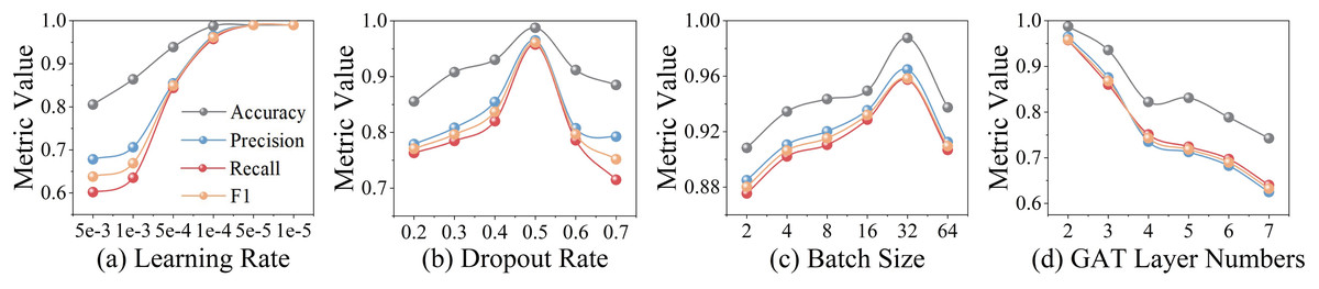
Figure 6: Evaluate the influence of hyperparameter settings on the performance of TransGraphNet.
(A) Learning rate; (B) Dropout rate; (C) Batch size; (D) GAT layer numbers.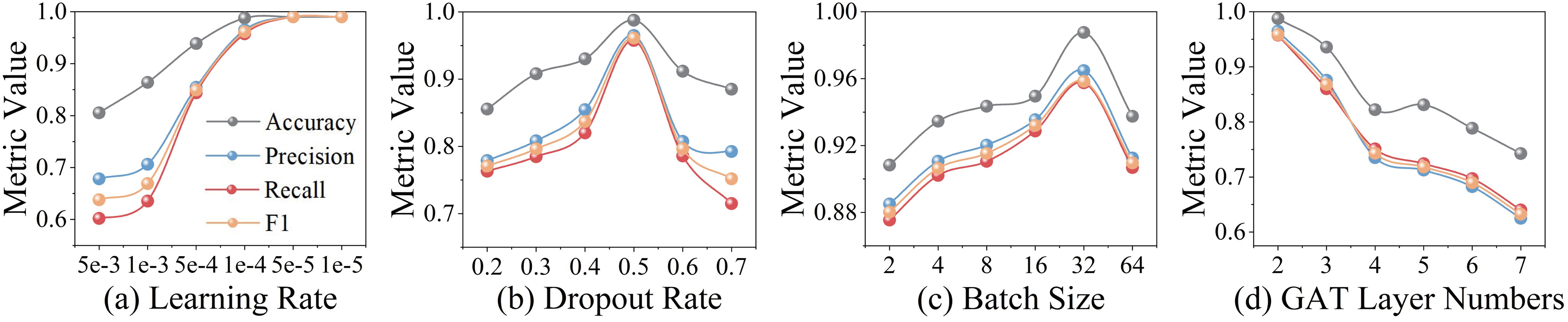

Download full-size image

DOI: 10.7717/peerj-cs.3353/fig-6

Overall performance evaluation (Q1)

To evaluate the performance of the proposed TransGraphNet model on the MTA dataset with traffic obfuscation and traditional encrypted traffic datasets without obfuscation, we select seven baselines based on statistical method, graph learning, and deep learning for comparative experiments. Detailed experimental results are presented in Table 5. Overall, TransGraphNet shows significant advantages across four metrics on the three datasets. Specifically, on the MTA dataset, TransGraphNet attains the highest accuracy of 0.9876 and an F1-score of 0.9611, outperforming the ET-BERT by 5.4% in accuracy and 6.8% in F1-score. This improvement is mainly due to the AFG module’s ability to model inter-flow relationships such as concurrency and trigger patterns, which remain effective even when individual flows are obfuscated. Unlike ET-BERT, which focuses solely on sequence patterns within a single flow, TransGraphNet captures broader structural behaviors across multiple flows in a session, thus enhancing robustness under obfuscation. On the CIC-IOT-2023 dataset, TransGraphNet improves accuracy and F1-score by 13.1% and 52.3%, respectively, compared to the AppScanner. In the binary classification task on the Stratosphere dataset, TransGraphNet achieves metrics of 0.99. A comparison with the baselines is provided below.

Comparison with statistical methods: AppScanner constructs a random forest classifier by extracting the 40 most relevant statistical features (Taylor et al., 2016), achieving an accuracy of 0.8623 on the CIC dataset. However, its accuracy on the MTA dataset is only 0.6902, indicating that relying solely on statistical features is insufficient to effectively capture the complex patterns of traffic. Although the BIND method incorporates bidirectional burst features for classification (Al-Naami et al., 2016), its accuracy and F1-score on the MTA dataset only improve by 2.2% and 10.7% over AppScanner, still failing in capturing complex traffic behaviors. In contrast, TransGraphNet integrates the temporal and spatial features of traffic, demonstrating more stable performance across different datasets. Notably, on the MTA dataset, its F1-score reaches 0.9611, significantly surpassing these statistical methods.
Comparison with graph-based methods: FG-Net employs a fixed time window for graph construction, which inadequately considers the dynamic variations in traffic (Jiang et al., 2022), thereby limiting its ability to accurately distinguish the behavior patterns of each category in multi-classification tasks. Therefore, its accuracy on the MTA and CIC datasets is 2.5% and 2.6% lower than the GraphDApp, respectively. However, GraphDApp focuses solely on packet-level information, failing to integrate flow-level data effectively (Shen et al., 2019). Consequently, in the binary classification tasks that demand high precision, its accuracy and F1-score on the Stratosphere dataset are respectively 4.4% and 4.2% lower than FG-Net. In contrast, TransGraphNet applies an adaptive sliding window for graph construction and considers multi-granularity features at both the packet and flow levels, achieving optimal performance across all three datasets.
Comparison with deep learning methods. FS-Net (Liu et al., 2019) and DF (Sirinam et al., 2018) overlook dynamic behavior patterns of traffic, resulting in F1-scores on the MTA dataset being 25.7% and 44.8% lower than TransGraphNet, respectively. ET-BERT uses a pre-trained Transformer architecture that enables self-learning from large-scale unlabeled data (Lin et al., 2022). Our proposed TransGraphNet similarly utilizes this architecture for modeling time series features, while incorporating CNN for statistical features, and uses GAT to obtain global representations. Although ET-BERT attains slightly higher accuracy and F1-scores than TransGraphNet on the binary classification Stratosphere dataset, its accuracy and F1-score on the multi-classification MTA dataset are 5.1% and 6.4% lower than TransGraphNet, respectively. Its performance on the CIC dataset also lags behind TransGraphNet. This shows that TransGraphNet effectively improves performance in multi-class scenarios of encrypted traffic through spatial-temporal feature fusion. To further analyze the classification behavior of TransGraphNet and its robustness against noisy traffic, we present the confusion matrices for both ET-BERT and TransGraphNet on the MTA dataset in Fig. 7. The results show that TransGraphNet achieves better class discrimination with fewer false positives, especially in the presence of obfuscated or noisy traffic, demonstrating its superior robustness in complex multi-class scenarios.

Table 5:

Compare model performance with baselines on MTA, CIC-IOT-2023, and Stratosphere datasets.

Category	Baseline	MTA				CIC-IOT-2023				Stratosphere
Category	Baseline	AC (% $\pm$ std)	PR (% $\pm$ std)	RC (% $\pm$ std)	F1 (% $\pm$ std)	AC (% $\pm$ std)	PR (% $\pm$ std)	RC (% $\pm$ std)	F1 (% $\pm$ std)	AC (% $\pm$ std)	PR (% $\pm$ std)	RC (% $\pm$ std)	F1 (% $\pm$ std)
Statistical	AppScanner	69.0 $\pm$ 1.8	41.2 $\pm$ 1.3	45.0 $\pm$ 1.5	43.0 $\pm$ 2.1	86.2 $\pm$ 1.4	60.3 $\pm$ 1.0	63.5 $\pm$ 1.2	61.9 $\pm$ 1.7	91.4 $\pm$ 0.9	91.6 $\pm$ 0.8	92.0 $\pm$ 0.8	91.8 $\pm$ 1.0
Statistical	BIND	70.5 $\pm$ 1.5	45.2 $\pm$ 1.2	50.3 $\pm$ 1.3	47.6 $\pm$ 1.8	85.5 $\pm$ 1.3	61.8 $\pm$ 1.1	64.3 $\pm$ 1.1	63.0 $\pm$ 1.5	92.6 $\pm$ 0.8	89.0 $\pm$ 0.9	89.9 $\pm$ 0.9	89.4 $\pm$ 0.9
Graph learning	GraphDApp	91.1 $\pm$ 0.7	70.7 $\pm$ 0.6	73.5 $\pm$ 0.8	72.1 $\pm$ 1.0	95.2 $\pm$ 0.6	91.4 $\pm$ 0.5	92.0 $\pm$ 0.5	91.7 $\pm$ 0.7	94.0 $\pm$ 0.6	92.0 $\pm$ 0.6	92.9 $\pm$ 0.6	92.5 $\pm$ 0.7
Graph learning	FG-Net	88.9 $\pm$ 0.8	72.5 $\pm$ 0.7	81.5 $\pm$ 0.9	76.7 $\pm$ 1.1	92.7 $\pm$ 0.7	86.3 $\pm$ 0.6	87.5 $\pm$ 0.6	86.9 $\pm$ 0.8	98.7 $\pm$ 0.3	96.4 $\pm$ 0.4	96.7 $\pm$ 0.4	96.5 $\pm$ 0.4
Deep learning	ET-BERT	93.6 $\pm$ 0.4	89.7 $\pm$ 0.5	90.3 $\pm$ 0.5	90.0 $\pm$ 0.5	96.6 $\pm$ 0.4	93.8 $\pm$ 0.4	94.5 $\pm$ 0.4	94.1 $\pm$ 0.5	99.6 $\pm$ 0.2	99.1 $\pm$ 0.3	99.4 $\pm$ 0.2	99.2 $\pm$ 0.2
	FS-Net	88.4 $\pm$ 0.6	69.7 $\pm$ 0.6	73.0 $\pm$ 0.7	71.3 $\pm$ 0.8	90.8 $\pm$ 0.5	87.3 $\pm$ 0.6	87.6 $\pm$ 0.5	87.4 $\pm$ 0.6	94.4 $\pm$ 0.3	92.0 $\pm$ 0.5	92.2 $\pm$ 0.5	92.5 $\pm$ 0.4
	DF	78.5 $\pm$ 1.2	50.3 $\pm$ 1.1	56.1 $\pm$ 1.2	53.1 $\pm$ 1.5	84.7 $\pm$ 1.0	64.9 $\pm$ 0.9	65.8 $\pm$ 1.0	65.4 $\pm$ 1.2	93.8 $\pm$ 0.6	91.3 $\pm$ 0.6	92.0 $\pm$ 0.6	91.6 $\pm$ 0.7
TransGraphNet		98.7 $\pm$ 0.2	96.4 $\pm$ 0.3	95.7 $\pm$ 0.3	96.1 $\pm$ 0.3	97.5 $\pm$ 0.2	92.7 $\pm$ 0.3	95.8 $\pm$ 0.3	94.2 $\pm$ 0.3	99.0 $\pm$ 0.2	99.3 $\pm$ 0.2	99.1 $\pm$ 0.2	99.2 $\pm$ 0.2

DOI: 10.7717/peerj-cs.3353/table-5

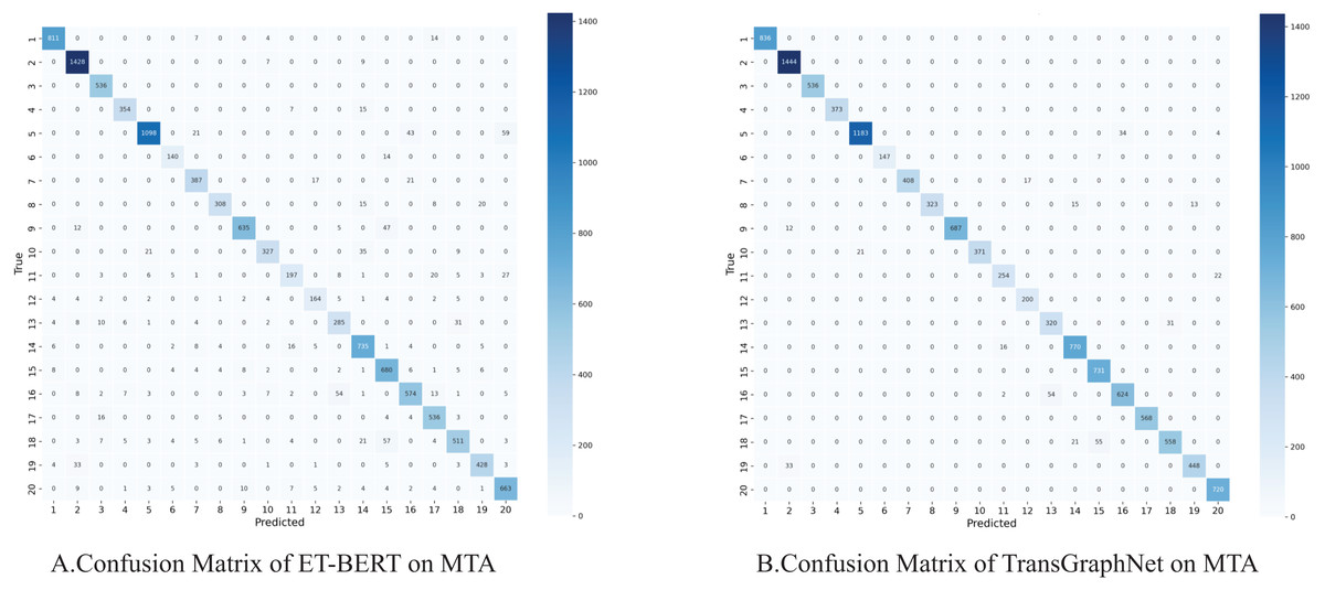
Figure 7: Comparison of confusion matrices for (A) ET-BERT and (B) TransGraphNet on the MTA dataset.

Download full-size image

DOI: 10.7717/peerj-cs.3353/fig-7

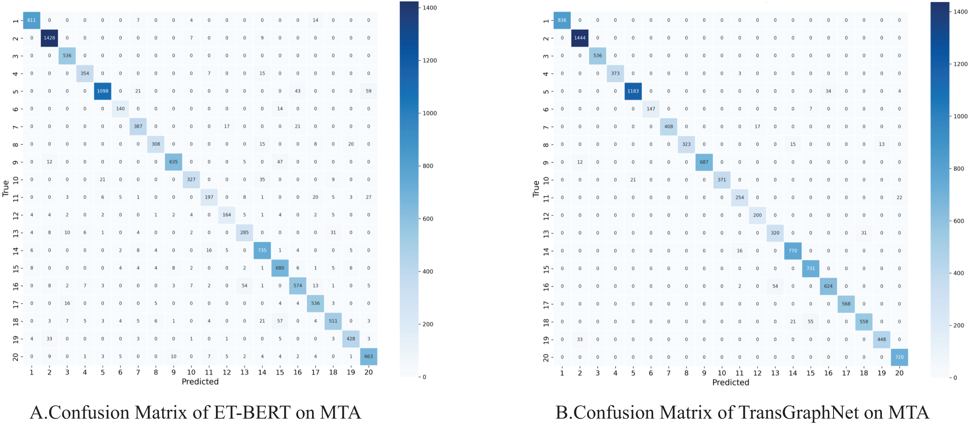
Ablation study and results (Q2)

To answer Q2, we conduct ablation experiments to evaluate the contribution of each module to overall performance by comparing the effects of four TransGraphNet variants on three datasets. The experimental results are presented in Table 6 and the detailed analysis is as follows:

Effectiveness of CNN module: After removing the CNN module, the performance of TransGraphNet-Without-CNN degrades on all three datasets, particularly on the MTA dataset, where accuracy and F1-scores drop by 13.1% and 25.1%, respectively. On the CIC dataset, precision and recall reduce by 13.7% and 13.1%, respectively. Although there is only a slight decline in performance on the binary-class Stratosphere dataset, the results still demonstrate that the CNN module is crucial for handling multi-class tasks.
Effectiveness of BERT module: After removing the BERT module, the performance of TransGraphNet-Without-BERT drops most significantly compared to the other three variants, particularly on the MTA dataset, where accuracy drops by 19.3% and F1-score by 28.4%. This shows that using BERT to capture long-range dependencies in time series features can significantly improve the model’s performance. Furthermore, Fig. 8 presents self-attention heatmaps from the final training epoch for both packet length and arrival time delta sequences. The packet-length attention demonstrates a globally distributed pattern, suggesting that the model integrates information from all positions. In contrast, the arrival-time attention reveals strong localized peaks, indicating that specific time intervals are more influential. These distinct attention behaviors highlight the BERT module’s capacity to capture heterogeneous temporal and structural dependencies, thus contributing to performance improvements observed in ablation studies.
Effectiveness of the attention mechanism: While replacing GAT with GCN in TransGraphNet-Replace-GCN led to a performance drop, the decline is less significant compared to the previous two variants. For instance, on the MTA dataset, accuracy decreased by only 6.5%, and the F1-score dropped by 7.3%. This suggests that GAT with an attention mechanism is more effective than GCN at capturing key features in the graph’s spatial topology.
Effectiveness of improved PLD algorithm: After removing the PLD module, TransGraphNet-Without-PLD exhibits a great performance drop on the MTA dataset than the other two datasets. The decline is particularly noticeable in precision and recall, which decrease by 13.5% and 11.4%, respectively. This indicates that the improved PLD algorithm can help the model maintain higher precision and recall by effectively handling time series features, thereby mitigating the impact of passive traffic obfuscation.

Table 6:

Evaluation of component contributions via ablation study on selected datasets.

Dataset	MTA				CIC-IOT-2023				Stratosphere				CIC-AndMal-2017
Variant	AC	PR	RC	F1	AC	PR	RC	F1	AC	PR	RC	F1	AC	PR	RC	F1
TransGraphNet-Without-BERT	0.796	0.687	0.689	0.688	0.895	0.774	0.793	0.783	0.938	0.865	0.878	0.871	0.470	0.463	0.469	0.398
TransGraphNet-Replace-GCN	0.923	0.891	0.891	0.891	0.933	0.864	0.883	0.874	0.944	0.889	0.901	0.895	0.798	0.869	0.780	0.806
TransGraphNet-Without-PLD	0.912	0.835	0.848	0.841	0.948	0.926	0.937	0.931	0.957	0.907	0.922	0.915	0.736	0.768	0.710	0.721
TransGraphNet (Ours)	0.987	0.964	0.957	0.961	0.975	0.927	0.958	0.942	0.990	0.993	0.991	0.992	0.804	0.899	0.782	0.813

DOI: 10.7717/peerj-cs.3353/table-6

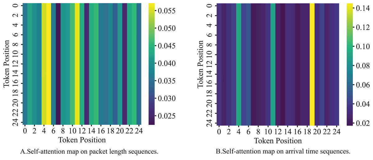
Figure 8: Visualization of attention weights from the BERT module in the final epoch on the MTA dataset.
Each map reflects how the model attends to different token positions within input sequences: (A) Self-attention map on packet length sequences; (B) Self-attention map on arrival time sequences.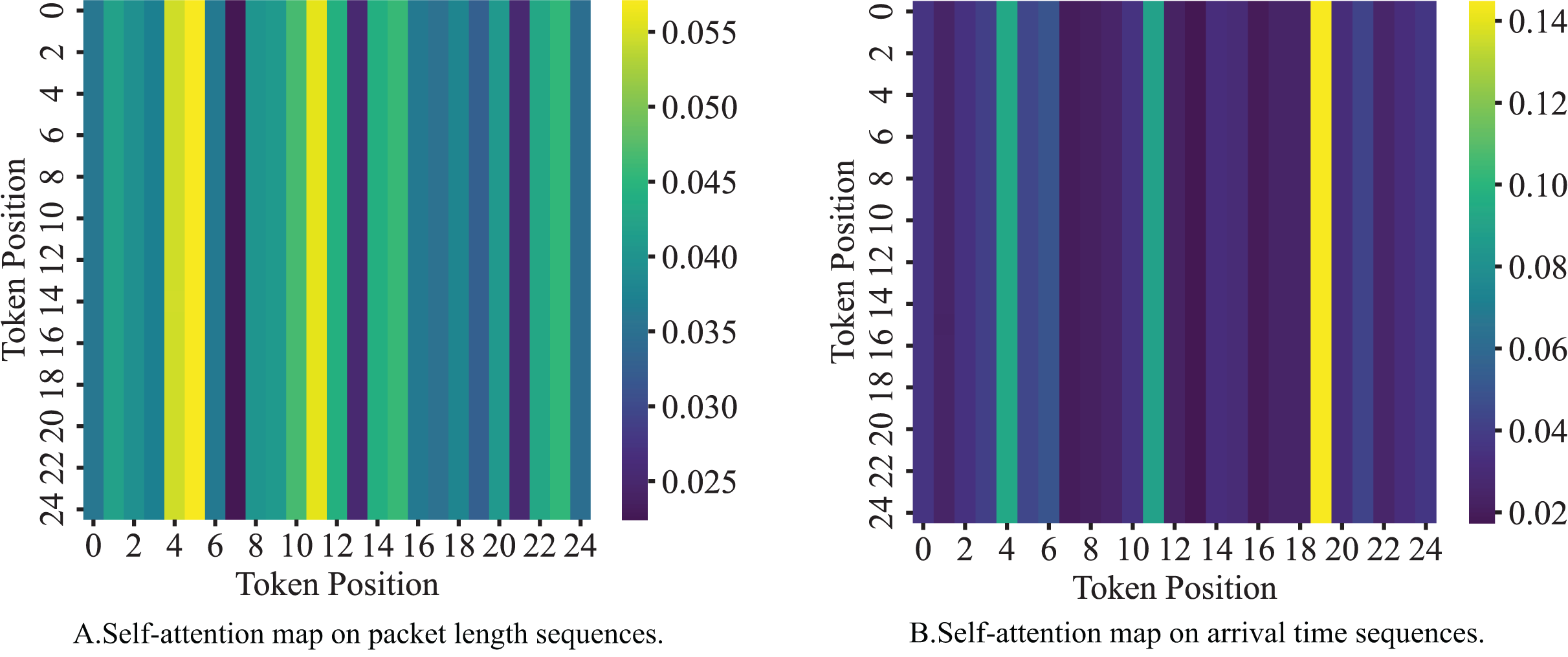

Download full-size image

DOI: 10.7717/peerj-cs.3353/fig-8

Overall, removing any module significantly affects TransGraphNet’s performance, indicating that each module is both effective and indispensable. Their synergy is crucial to the model’s ultimate performance.

Experiments on two window mechanisms (Q3)

To effectively answer Q3 and investigate which windowing mechanism better captures the dynamic characteristics of malicious encrypted traffic, we comprehensively compare the fixed time window and the proposed Adaptive Sliding Window (ASW) approach. We begin by visualizing flow-level graphs constructed using both mechanisms to assess their ability to preserve burst semantics across representative traffic types. We then quantitatively evaluate their classification performance on the MTA dataset under different window sizes. Finally, we perform sensitivity analysis on key parameters in ASW, including the inter-flow threshold $δ$ , maximum window size $T_{m a x}$ , packet length vocabulary size $k$ , and regularization interval $Δ τ^{'}$ , to determine their optimal settings and justify the design choices of the adaptive window.

Graph construction comparison: In Fig. 9, vertices of the same color represent the same burst flow, vertices within a burst are connected by dashed lines and solid lines linking different bursts. In the case of Trickbot, the fixed window incorrectly includes Flow 7, which does not align with Trickbot’s typical behavior pattern. In contrast, the adaptive sliding window accurately identifies the dynamic changes in the traffic and excludes Flow 7. For Qakbot, CobaltStrike, and Emotet, the fixed window misses subsequent burst behaviors, whereas the adaptive sliding window can capture these behaviors, addressing the issue of missing interaction topology information under fixed time windows graph construction. Note that different types of malware exhibit distinct attack patterns, resulting in varied flow-level burst graphs, highlighting the importance of graph construction in identifying traffic patterns.
Performance comparison: As shown in Fig. 10, with the fixed window size increasing from 30 to 90 s, the performance on the MTA dataset gradually improves and peaks at 90 s. However, the accuracy and F1-scores remain 7.8% and 8.9% lower than the adaptive sliding window (ASW) when the fixed window size is set to 90 s. Subsequently, when the window size reaches 120 s, the model’s performance significantly declines. This indicates that both shorter and longer fixed window sizes struggle to accurately capture the dynamic behavior patterns of malicious encrypted traffic. In contrast, the adaptive sliding window can automatically adjust the window size based on the time intervals between traffic flows, thereby better capturing dynamic behavior patterns.

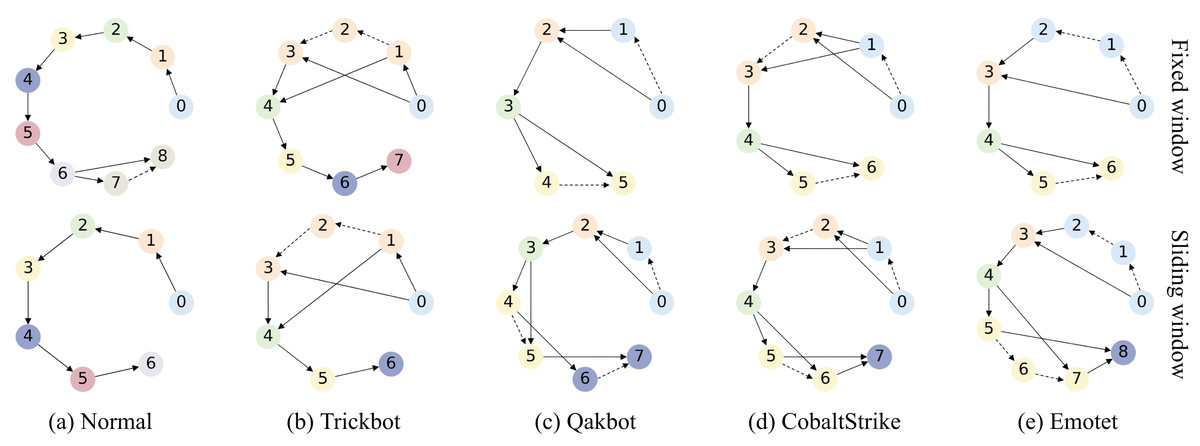
Figure 9: Differences in flow relation graphs built with a fixed 90-s window and a sliding window.
(A) Normal; (B) Trickbot; (C) Qakbot; (D) CobaltStrike; (E) Emotet.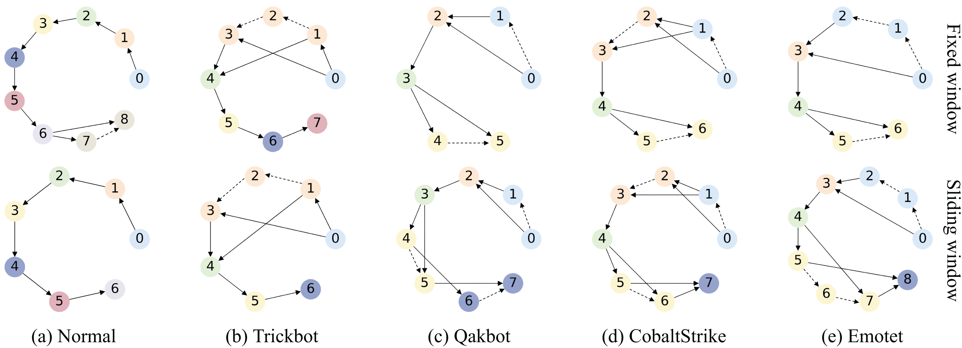

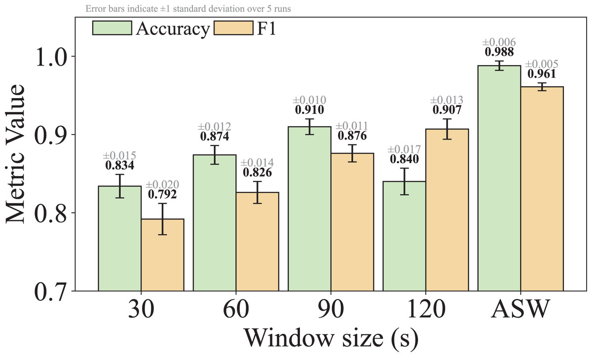
Download full-size image

DOI: 10.7717/peerj-cs.3353/fig-9

Figure 10: Evaluating the performance of our model under varying time window sizes.

Download full-size image

DOI: 10.7717/peerj-cs.3353/fig-10

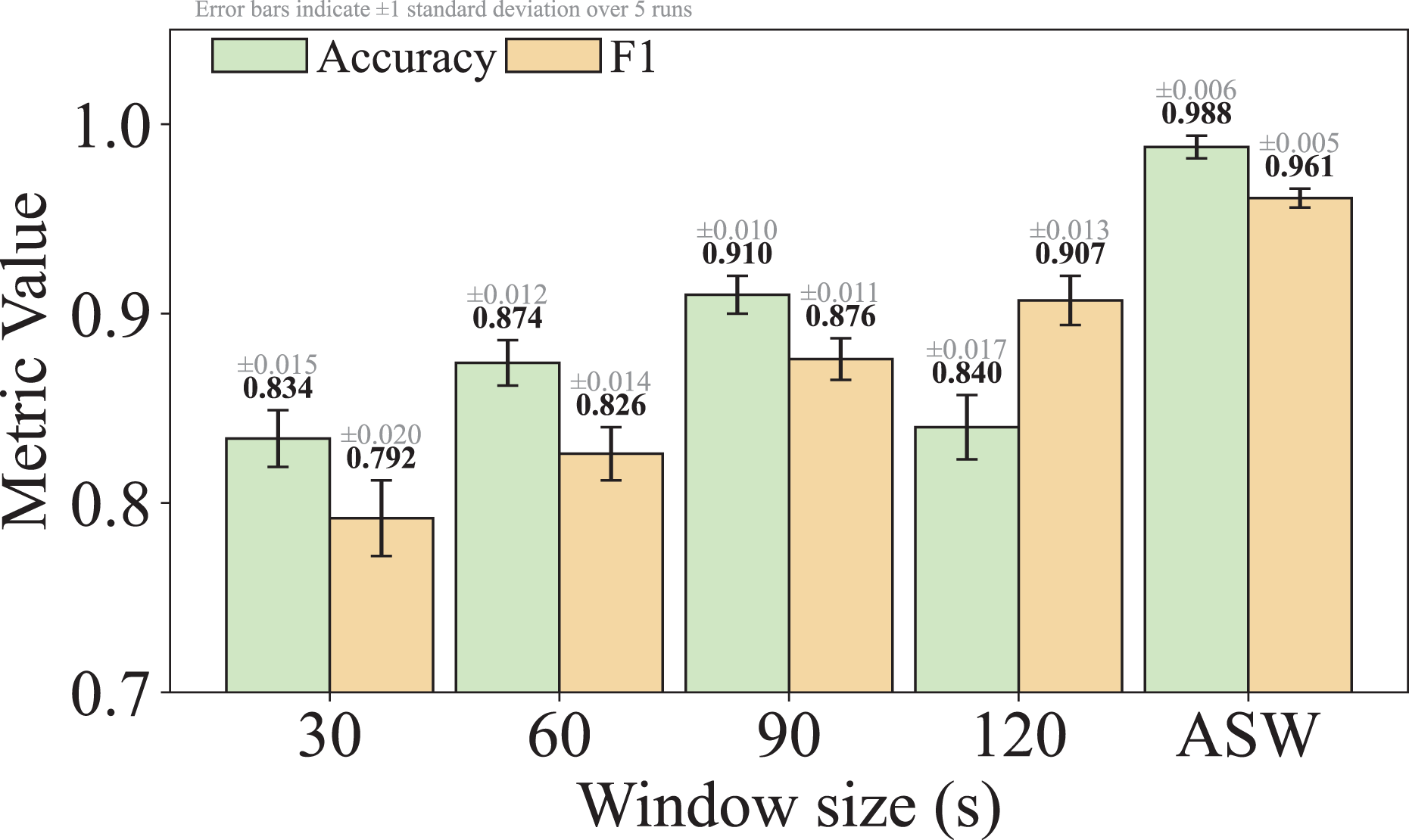
We further conduct sensitivity analysis on the inter-flow threshold $δ$ , which controls the granularity of burst segmentation in our Adaptive Sliding Window mechanism. As shown in Fig. 11, performance peaks at $δ = 10$ with 98.70% accuracy and 96.10% macro F1. Small values such as $δ = 1$ or 5 lead to fragmented bursts and degraded performance due to loss of contextual information. Larger values such as 15 or 20 slightly reduce accuracy and F1, likely because they merge unrelated bursts. We select $δ = 10$ as the default for optimal trade-off between burst granularity and model performance.

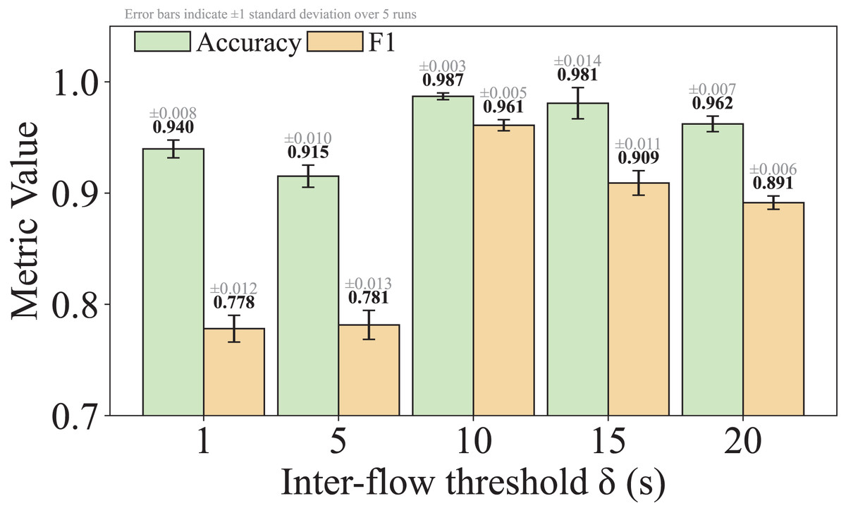
Evaluating the performance of our model under varying inter-flow threshold
${\delta}$δ
. — Figure 11: Evaluating the performance of our model under varying inter-flow threshold $δ$ .

Download full-size image

DOI: 10.7717/peerj-cs.3353/fig-11

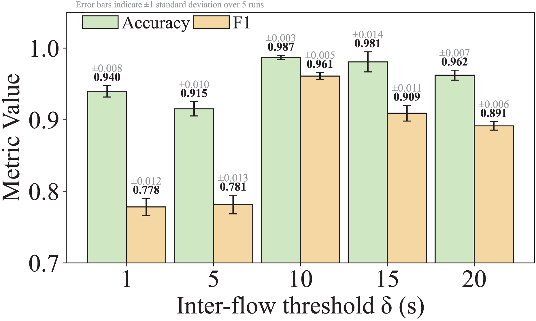
Figure 12 shows the sensitivity analysis on the parameter $T_{m a x}$ . When $T_{m a x} = 150$ , the model achieves the best performance with 98.70% accuracy and 96.10% macro F1, suggesting that this window size effectively balances temporal context and noise suppression. A smaller window such as $T_{m a x} = 50$ still yields strong results, but may cause session fragmentation and loss of context. In contrast, $T_{m a x} = 100$ leads to a sharp performance drop, likely due to insufficient burst coverage. Larger windows like 200 and 250 maintain high scores but show slight declines. We select $T_{m a x} = 150$ as the optimal setting.

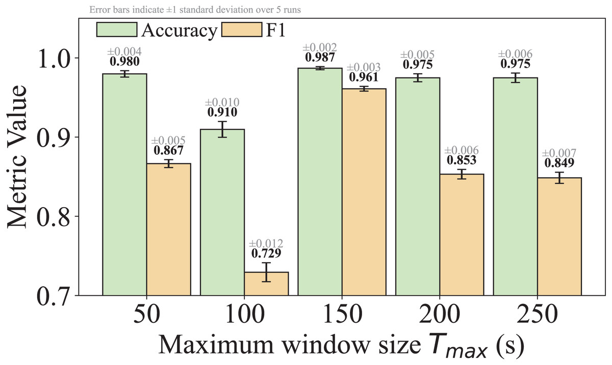
Evaluating the performance of our model under varying maximum window size
${{ T}_{ max}}$Tmax
. — Figure 12: Evaluating the performance of our model under varying maximum window size $T_{m a x}$ .

Download full-size image

DOI: 10.7717/peerj-cs.3353/fig-12

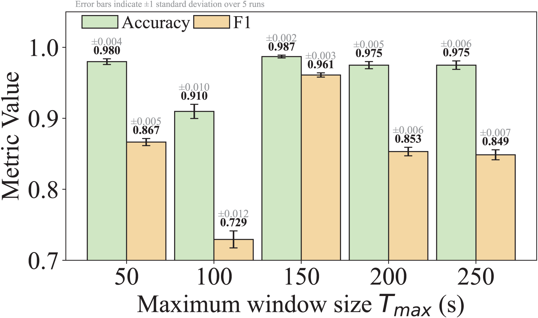
To standardize packet length sequences while preserving protocol semantics, we extract the top- $k$ most frequent packet lengths per traffic category. The parameter $k$ controls how many high-frequency values are retained during standardization. As shown in Fig. 13, increasing $k$ from 10 to 20 significantly improves performance, reaching 98.70% accuracy and 96.10% macro F1. However, performance drops at $k = 30$ , suggesting that overly large vocabularies may introduce noise. Accuracy recovers at $k = 40$ and $k = 50$ , but the gains are marginal. We choose $k = 20$ as the default, offering the best trade-off between performance and generalization.

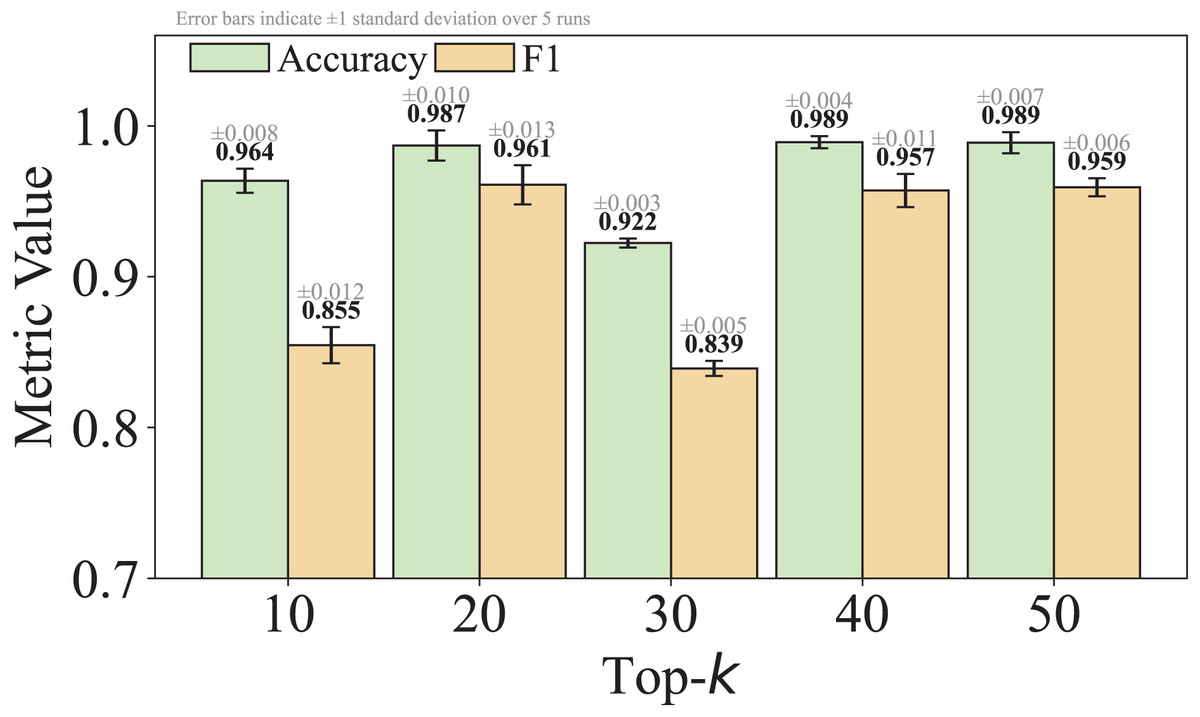
Figure 13: Evaluating the performance of our model under varying top-k most frequent lengths.

Download full-size image

DOI: 10.7717/peerj-cs.3353/fig-13

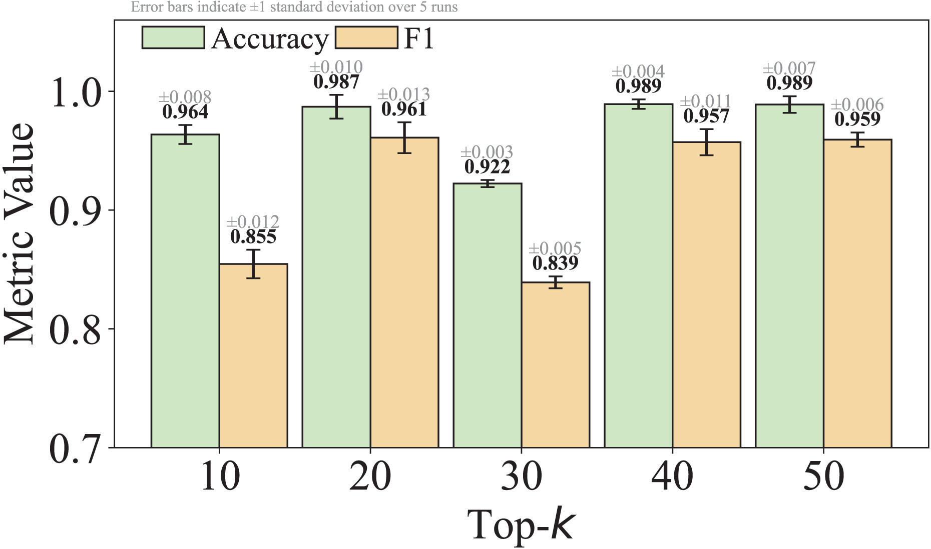
To evaluate the impact of the rounding threshold $Δ τ^{'}$ , we conducted a sensitivity analysis by varying $Δ τ^{'}$ from 1 to 9, as illustrated in Fig. 14. The results show that performance improves as $Δ τ^{'}$ increases, peaking at $Δ τ^{'} = 7$ , where both accuracy and macro F1-score reach 98.70% and 96.10%, respectively. Too small values introduce noise, while overly large values may oversimplify packet representations. Therefore, we choose $Δ τ^{'} = 7$ as the default setting for optimal balance.

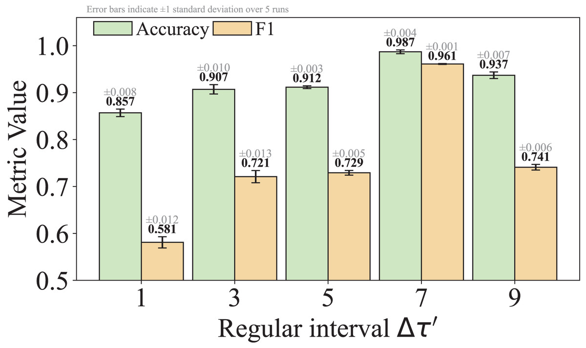
Evaluating the performance of our model under varying regular interval
${\Delta} {\tau}^{\prime}$Δτ′
. — Figure 14: Evaluating the performance of our model under varying regular interval $Δ τ^{'}$ .

Download full-size image

DOI: 10.7717/peerj-cs.3353/fig-14

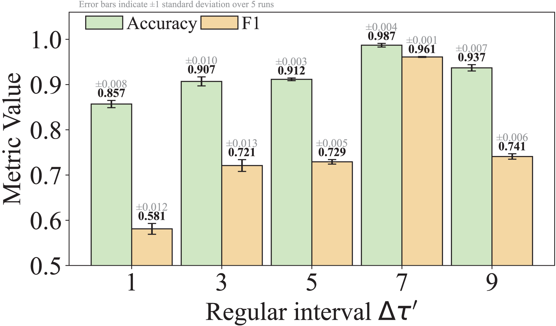
Evaluation of TransGraphNet’s robustness (Q4)

To assess the robustness of TransGraphNet in detecting malicious encrypted traffic with obfuscation, we calculate the recall (RC) and F1-scores of TransGraphNet, GraphDApp (Shen et al., 2019), and ET-BERT (Koroteev, 2021) across 20 categories in the MTA dataset, where ten categories are malicious encrypted traffic without obfuscation and ten categories are obfuscated malicious encrypted traffic. This includes CobaltStrike, known for its active traffic obfuscation methods, and Emote (Trickbot), which is mixed with noise traffic generated by Trickbot due to passive obfuscation. The results are presented in Table 7 and are analyzed as follows:

Robustness against active traffic obfuscation: TransGraphNet demonstrates the best multi-class performance on the MTA dataset. For the ten categories without traffic obfuscation, TransGraphNet achieves the highest recall and F1-scores in the same nine categories, while ET-BERT leads in Trickster categories. For the CobaltStrike category, due to its active traffic obfuscation methods, the recall and F1-score for ET-BERT is only 78.4% and 78.6%, respectively. In contrast, TransGraphNet surpasses ET-BERT by 9.8% and 9.7% on these two metrics.
Robustness against passive traffic obfuscation: For the nine categories of obfuscated traffic resulting from multi-stage attacks, TransGraphNet attains the highest recall and F1-scores, exceeding 83%, whereas GraphDAPP performs significantly worse, with recall and F1-scores below 70%.
Robustness under simulated noise: To further validate TransGraphNet’s robustness against time series noise interference, we incrementally select two categories from the ten non-obfuscated malicious encrypted traffic categories in the MTA dataset and introduce random perturbations within $\pm$ 10% to the packet length sequence of these categories to simulate realistic network conditions. The experimental results in Fig. 15 show that when the number of noisy categories increases from 9 to 19, TransGraphNet demonstrates only a minor decline in accuracy, with precision and recall remaining above 92% and F1-score staying stable.

Table 7:

Comparison of model performance on MTA dataset in recall and F1-score.

Category	RC (% $\pm$ std)			F1 (% $\pm$ std)
	Graph DAPP	ET-BERT	Ours	Graph DAPP	ET-BERT	Ours
Artemis	69.2 $\pm$ 2.1	86.2 $\pm$ 1.3	89.2 $\pm$ 0.8	68.1 $\pm$ 2.3	87.3 $\pm$ 1.1	88.9 $\pm$ 0.7
Barys	70.1 $\pm$ 1.9	83.9 $\pm$ 1.5	92.6 $\pm$ 0.7	71.1 $\pm$ 1.8	84.2 $\pm$ 1.4	91.2 $\pm$ 0.6
Bokbot	69.2 $\pm$ 2.0	84.4 $\pm$ 1.4	92.8 $\pm$ 0.6	66.8 $\pm$ 2.1	83.7 $\pm$ 1.5	94.9 $\pm$ 0.5
Danabot	68.6 $\pm$ 2.2	84.6 $\pm$ 1.3	94.2 $\pm$ 0.5	66.0 $\pm$ 2.4	83.2 $\pm$ 1.6	95.7 $\pm$ 0.4
Emotet	65.2 $\pm$ 2.5	86.7 $\pm$ 1.2	96.9 $\pm$ 0.4	65.2 $\pm$ 2.5	87.0 $\pm$ 1.1	96.8 $\pm$ 0.4
Trickbot	72.3 $\pm$ 1.8	83.2 $\pm$ 1.6	94.2 $\pm$ 0.5	72.6 $\pm$ 1.7	82.4 $\pm$ 1.7	94.9 $\pm$ 0.4
Trickster	59.2 $\pm$ 3.0	94.3 $\pm$ 0.8	91.2 $\pm$ 0.9	57.2 $\pm$ 3.2	94.8 $\pm$ 0.7	92.8 $\pm$ 0.8
Ursnif	57.2 $\pm$ 3.2	84.6 $\pm$ 1.4	99.4 $\pm$ 0.3	61.2 $\pm$ 2.9	84.3 $\pm$ 1.5	98.8 $\pm$ 0.4
Qakbot	68.6 $\pm$ 2.1	86.4 $\pm$ 1.2	94.2 $\pm$ 0.5	65.8 $\pm$ 2.3	87.5 $\pm$ 1.0	94.9 $\pm$ 0.4
Normal	79.2 $\pm$ 1.5	90.8 $\pm$ 0.9	98.2 $\pm$ 0.3	79.2 $\pm$ 1.5	93.2 $\pm$ 0.7	97.8 $\pm$ 0.3
CobaltStrike	59.2 $\pm$ 3.1	78.4 $\pm$ 1.8	88.2 $\pm$ 1.0	59.6 $\pm$ 3.0	78.6 $\pm$ 1.7	88.3 $\pm$ 0.9
Pikabot (C.S.)	59.2 $\pm$ 3.0	85.3 $\pm$ 1.3	89.6 $\pm$ 0.9	57.6 $\pm$ 3.1	87.6 $\pm$ 1.1	89.8 $\pm$ 0.8
BazarLoader (C.S.)	62.2 $\pm$ 2.8	84.3 $\pm$ 1.4	88.7 $\pm$ 0.9	60.2 $\pm$ 2.9	84.3 $\pm$ 1.4	88.5 $\pm$ 0.9
Bokbot (C.S.)	62.6 $\pm$ 2.7	82.3 $\pm$ 1.6	88.8 $\pm$ 0.9	59.8 $\pm$ 2.8	83.2 $\pm$ 1.5	88.9 $\pm$ 0.8
Bumblebee (C.S.)	65.2 $\pm$ 2.5	81.2 $\pm$ 1.7	87.8 $\pm$ 1.0	63.2 $\pm$ 2.6	81.2 $\pm$ 1.7	87.6 $\pm$ 1.0
Hancitor (C.S.)	64.2 $\pm$ 2.6	80.0 $\pm$ 1.8	89.7 $\pm$ 0.8	64.2 $\pm$ 2.6	78.3 $\pm$ 1.9	89.6 $\pm$ 0.8
Emote (C.S.)	63.2 $\pm$ 2.7	81.7 $\pm$ 1.7	87.4 $\pm$ 1.0	68.2 $\pm$ 2.3	79.2 $\pm$ 1.8	83.1 $\pm$ 1.2
Emotet (Spambot)	61.2 $\pm$ 2.9	81.3 $\pm$ 1.7	89.7 $\pm$ 0.8	59.2 $\pm$ 3.0	84.1 $\pm$ 1.5	88.6 $\pm$ 0.9
Emotet (Trickbot)	62.2 $\pm$ 2.8	80.2 $\pm$ 1.8	87.0 $\pm$ 1.1	62.2 $\pm$ 2.8	83.4 $\pm$ 1.6	86.2 $\pm$ 1.1
Bunitu (Botnet)	67.2 $\pm$ 2.4	81.6 $\pm$ 1.7	86.6 $\pm$ 1.1	65.2 $\pm$ 2.5	81.3 $\pm$ 1.7	85.3 $\pm$ 1.2

DOI: 10.7717/peerj-cs.3353/table-7

Figure 15: Evaluating the performance of our model under varying numbers of noisy classes.

Download full-size image

DOI: 10.7717/peerj-cs.3353/fig-15

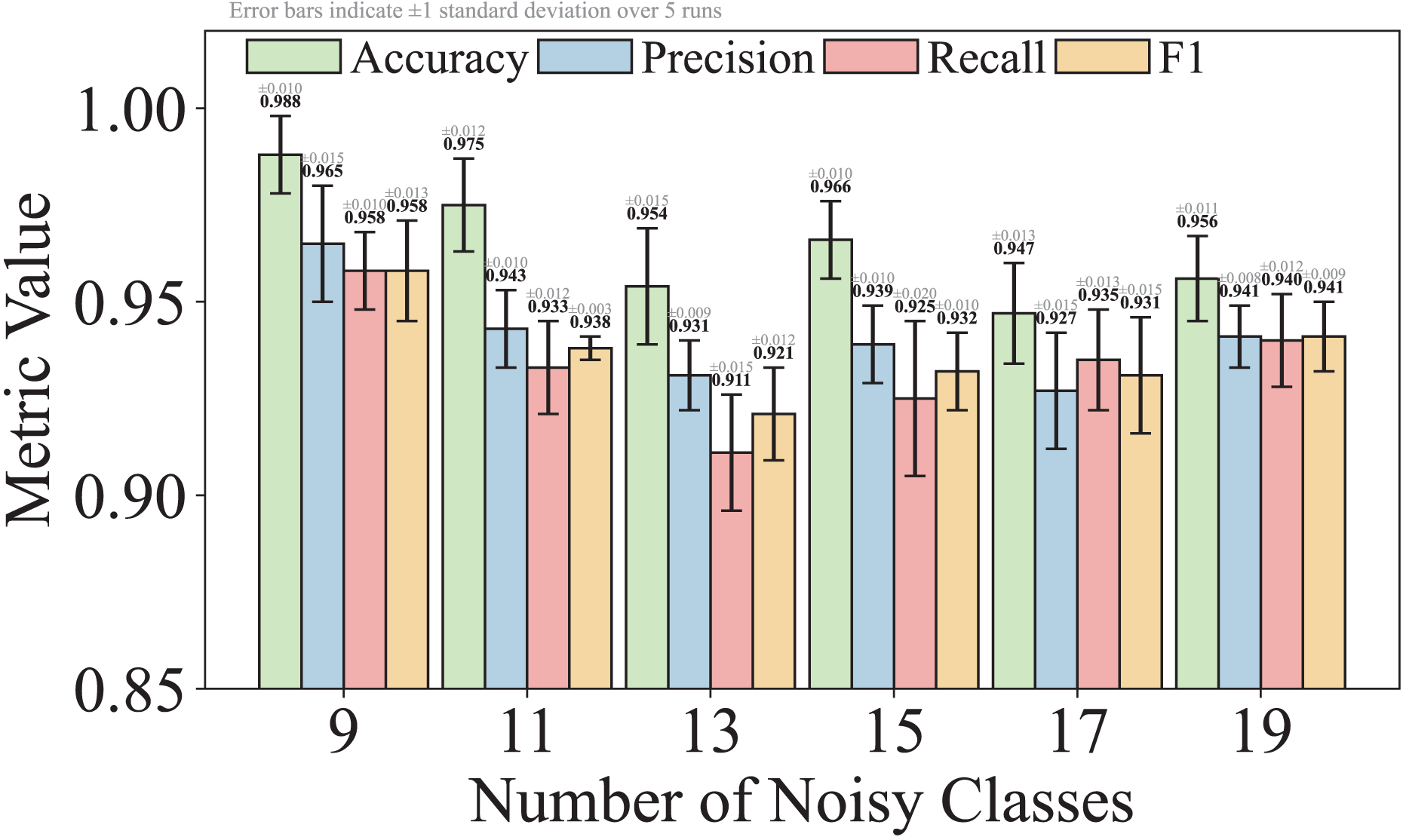
The results show TransGraphNet’s strong robustness against malicious encrypted traffic with obfuscation, while also validating the effectiveness of the improved PLD algorithm in processing time series.

Discussion about future research

In this section, we analyze the limitations of TransGraphNet and discuss our future research directions.

Challenges of fully encrypted traffic. TransGraphNet mainly focuses on analyzing encrypted traffic using the TLS 1.2 protocol. However, as encryption technologies evolve, such as TLS 1.3 and QUIC protocol, both the client key exchange and server-finished messages are encrypted, significantly enhancing security. To address these challenges, future research will delve into side-channel characteristics and behavioral patterns to explore new detection methods.
Challenges in computing and storage. TransGraphNet is a multi-module architecture based on spatial-temporal feature fusion, increasing model complexity and the number of parameters. In particular, graph-based algorithms have high computational cost, which poses challenges during real-world deployment, especially on resource-constrained devices. Future research could explore the model compression techniques (e.g., knowledge distillation) to reduce the computational burden and parameter size.
Potential vulnerability to adversarial manipulations. While TransGraphNet incorporates strategies such as the PLD algorithm and spatial-temporal feature fusion to enhance robustness, it still partially relies on common burst patterns and temporal consistency in encrypted traffic. Hence, in future work, we will explore adversarial learning techniques, including adversarial training, invariant feature extraction, and behavior-aware modeling, to further improve TransGraphNet’s resilience against evasion attempts.

Conclusion

In this article, we address the challenge of robust detection of malicious encrypted traffic under obfuscation by proposing the TransGraphNet framework, which consists of three key components. First, the Power Law Division algorithm is used to standardize packet length features, enhancing the model’s robustness against passive traffic obfuscation. Second, an Adaptive Sliding Window Flow-level Burst Graph (AFG) is constructed for each client-server session window to capture the concurrency and trigger relationships among associated five-tuple flows. The concurrency relationship is derived using an adaptive sliding window algorithm (rather than a fixed time window) to preserve critical interaction information, which is inherently difficult to manipulate through active obfuscation. Third, a hybrid transformer-GNN model is employed to fuse the spatial and temporal features of the AFG, thereby improving the model’s representational capacity. Experimental results demonstrate that TransGraphNet outperforms state-of-the-art methods (e.g., FG-Net, ET-BERT, GraphDApp) on the MTA with traffic obfuscation, improving accuracy by 11%, 5.4% and 6.8%, respectively, as well as on the CIC-IOT-2023 and Stratosphere datasets without obfuscation.

[1] Al-Naami K, Chandra S, Mustafa A, Khan L, Lin Z, Hamlen K, Thuraisingham B. 2016. Adaptive encrypted traffic fingerprinting with bi-directional dependence.

[2] Alshammari R, Zincir-Heywood AN. 2011. Can encrypted traffic be identified without port numbers, IP addresses and payload inspection? Computer Networks 55(6):1326-1350

[3] Bastos G, Marzano A, Fonseca O, Fazzion E, Hoepers C, Steding-Jessen K, Cunha Í, Guedes D, Meira W. 2019. Identifying and characterizing bashlite and mirai C&C servers.

[4] Bayat N, Jackson W, Liu D. 2021. Deep learning for network traffic classification. ArXiv

[5] CobaltStrike. 2024. Valid SSL certificates with SSL beacon.

[6] Dai R, Gao C, Lang B, Yang L, Liu H, Chen S. 2019. SSL malicious traffic detection based on multi-view features.

[7] Diao Z, Xie G, Wang X, Ren R, Meng X, Zhang G, Xie K, Qiao M. 2023. EC-GCN: a encrypted traffic classification framework based on multi-scale graph convolution networks. Computer Networks 224:109614

[8] Duncan B. 2024. MTA dataset: malware traffic analysis.

[9] Govindarajan V, Muzamal JH. 2025. Advanced cloud intrusion detection framework using graph based features transformers and contrastive learning. Scientific Reports 15(1):20511

[10] Hnamte V, Hussain J. 2023. Dependable intrusion detection system using deep convolutional neural network: a novel framework and performance evaluation approach. Telematics and Informatics Reports 11(9):100077

[11] Hu Z, Qu B, Li X, Li C. 2024. An encrypted traffic classification framework based on higher-interaction-graph neural network.

[12] Jiang M, Li Z, Fu P, Cai W, Cui M, Xiong G, Gou G. 2022. Accurate mobile-app fingerprinting using flow-level relationship with graph neural networks. Computer Networks 217(1):109309

[13] Keshkeh K, Jantan A, Alieyan K, Gana UM. 2021. A review on TLS encryption malware detection: Tls features, machine learning usage, and future directions.

[14] Koroteev MV. 2021. Bert: a review of applications in natural language processing and understanding. ArXiv

[15] Lakshmanan M, Adnan MM, Reddy RA, Vasukidevi G, Aarthy G. 2024. A graph neural network and transformer encoder technique for anomaly and cyber threat detection in smart grids.

[16] Lashkari AH, Kadir AFA, Taheri L, Ghorbani AA. 2018. Toward developing a systematic approach to generate benchmark android malware datasets and classification.

[17] Lee W, Jin S. 2021. Encrypted malware traffic detection using TLS features and random forest.

[18] Li W, Fu H, Han Z, Zhang X, Jin H. 2022. Intelligent tool wear prediction based on informer encoder and stacked bidirectional gated recurrent unit. Robotics and Computer-Integrated Manufacturing 77(1):102368

[19] Li W, Zhang X-Y, Bao H, Yang B, Li Z, Shi H, Wang Q. 2023. Prism: real-time privacy protection against temporal network traffic analyzers. IEEE Transactions on Information Forensics and Security 18:2524-2537

[20] Lin X, Xiong G, Gou G, Li Z, Shi J, Yu J. 2022. ET-BERT: a contextualized datagram representation with pre-training transformers for encrypted traffic classification.

[21] Liu C, Cao Z, Xiong G, Gou G, Yiu S-M, He L. 2018. MAMPF: encrypted traffic classification based on multi-attribute Markov probability fingerprints.

[22] Liu C, He L, Xiong G, Cao Z, Li Z. 2019. FS-Net: a flow sequence network for encrypted traffic classification.

[23] Liu J, Wang L, Hu W, Gao Y, Cao Y, Lin B, Zhang R. 2023. Spatial-temporal feature with dual-attention mechanism for encrypted malicious traffic detection. Security and Communication Networks 2023(1):7117863

[24] Lokoč J, Kohout J, Čech P, Skopal T, Pevnỳ T. 2016. k-NN classification of malware in HTTPS traffic using the metric space approach.

[25] Lotfollahi M, Jafari Siavoshani M, Shirali Hossein Zade R, Saberian M. 2020. Deep packet: a novel approach for encrypted traffic classification using deep learning. Soft Computing 24(3):1999-2012

[26] Mo Y, Li H, Wang D, Liu G. 2024. An intrusion detection system based on convolution neural network. PeerJ Computer Science 10(18):e2152

[27] Oudah H, Ghita B, Bakhshi T, Alruban A, Walker DJ. 2019. Using burstiness for network applications classification. Journal of Computer Networks and Communications 2019(1):5758437

[28] Piet J, Anderson B, McGrew D. 2018. An in-depth study of open-source command and control frameworks.

[29] Shen M, Zhang J, Zhu L, Xu K, Du X. 2021. Accurate decentralized application identification via encrypted traffic analysis using graph neural networks. IEEE TIFS 16:2367-2380

[30] Shen M, Zhang J, Zhu L, Xu K, Du X, Liu Y. 2019. Encrypted traffic classification of decentralized applications on ethereum using feature fusion.

[31] Sirinam P, Imani M, Juarez M, Wright M. 2018. Deep fingerprinting: undermining website fingerprinting defenses with deep learning.

[32] Sun W, Zhang Y, Li J, Sun C, Zhang S. 2022. A deep learning-based encrypted VPN traffic classification method using packet block image. Electronics 12(1):115

[33] Taylor VF, Spolaor R, Conti M, Martinovic I. 2016. Appscanner: automatic fingerprinting of smartphone apps from encrypted network traffic.

[34] The DFIR Report. 2021. Cobalt strike, a defender’s guide.

[35] Veličković P, Cucurull G, Casanova A, Romero A, Lio P, Bengio Y. 2017. Graph attention networks. ArXiv

[36] Wang H, Tang Z, Li H, Zhang J, Li S, Wang J. 2023. CI_GRU: an efficient DGA botnet classification model based on an attention recurrence plot. Computer Networks 235:109992

[37] Weng Z, Chen T, Zhu T, Dong H, Zhou D, Alfarraj O. 2021. TLSmell: direct identification on malicious https encryption traffic with simple connection-specific indicators. Computer Systems Science and Engineering 37(1):105-119

[38] Yang J, Jiang X, Lei Y, Liang W, Ma Z, Li S. 2024a. Mtsecurity: privacy-preserving malicious traffic classification using graph neural network and transformer. IEEE Transactions on Network and Service Management 21(3):3583-3597

[39] Yang Y, Li Z, Li Y, Cao T, Li Z. 2023. Stability enhancement for traffic flow via self–stabilizing control strategy in the presence of packet loss. Physica A: Statistical Mechanics and its Applications 622:128801

[40] Yang X, Ruan S, Yue Y, Sun B. 2024b. PETNet: plaintext-aware encrypted traffic detection network for identifying cobalt strike https traffics. Computer Networks 238:110120