
Defect text recognition and condition assessment method of power equipment based on BERT-BiLSTM
- Published
- Accepted
- Received
- Academic Editor
- Siddhartha Bhattacharyya
- Subject Areas
- Artificial Intelligence, Data Mining and Machine Learning, Natural Language and Speech, Optimization Theory and Computation, Text Mining
- Keywords
- Transformer defects, Text categorization, BERT-BiLSTM, Defect text
- Copyright
- © 2025 Shao et al.
- Licence
- This is an open access article distributed under the terms of the Creative Commons Attribution License, which permits unrestricted use, distribution, reproduction and adaptation in any medium and for any purpose provided that it is properly attributed. For attribution, the original author(s), title, publication source (PeerJ Computer Science) and either DOI or URL of the article must be cited.
- Cite this article
- 2025. Defect text recognition and condition assessment method of power equipment based on BERT-BiLSTM. PeerJ Computer Science 11:e3318 https://doi.org/10.7717/peerj-cs.3318
Abstract
The accumulated text of power equipment defects in operation are crucial for condition evaluation and maintenance. However, different structures of defect texts and their sensitivity to the experience of operation and maintenance personnel have led to difficulties in information mining, resulting in low efficiency of defect management. To address this issue, a defect text recognition method for power equipment is proposed based on Bidirectional Encoder Representations from Transformers-Bidirectional Long Short-Term Memory Neural Network (BERT-BiLSTM). First, the pre-training model of BERT is used to provide word vectors, which are fine-tuned by the BERT model based on the context of the defect text. Combined with the global semantic information, the vectors are inputted into the BiLSTM model. Then BiLSTM is used to encode and fuse features of the sequences to extract deep semantic features of defects. The obtained categories include defect severity, component, and type identification results. Based on algorithm comparison and case verification, the accuracy of the method is greater than 94% in identifying defect severity and component, proving the accurate recognition of defect text of power equipment. Finally, a defect condition assessment method is proposed to improve health management and condition maintenance.
Introduction
The intelligence of smart grid is developing increasingly. Digital empowerment integrates artificial intelligence and information technology with power systems, enhancing digital capabilities and transforming traditional operation and maintenance of equipment (Pu et al., 2020; Jina et al., 2024). Over long-term operation, transformers accumulate large amounts of structured and unstructured data, including text, audio, and images (Liu et al., 2022; Meng et al., 2023; Lu et al., 2023), which are crucial for status assessment and fault diagnosis (Liao et al., 2023; Li et al., 2021). Compared with audio and image data, manually recorded defect texts provide more precise defect information, but standardization is limited by personnel expertise, reducing text data utilization (Ge et al., 2021; Liu et al., 2023). Equipment health warning and fault diagnosis based on defect text mainly rely on manual processing, with decisions based on expert experience, leading to slow response times (Liu et al., 2019). Leveraging massive defect text for transformer condition assessment and maintenance is thus critical for improving operational efficiency (Jia et al., 2023).
Several studies have explored transformer defect text mining in power systems (Wei et al., 2017; Liu et al., 2018; Jiang et al., 2019; Feng et al., 2020; Wang et al., 2024). Wei et al. (2017) proposed an Recurrent Neural Network-Long Short-Term Memory (RNN-LSTM) method for fault classification, improving the handling of unstructured data. Liu et al. (2018) applied Convolutional Neural Network (CNN) for transformer defect text classification. Jiang et al. (2019) used an RCNN-based approach to evaluate equipment health from defect levels. Feng et al. (2020) introduced a Bidirectional Long Short-Term Memory Neural Network (BiLSTM) with attention mechanism, enhancing classification accuracy and proposing a defect priority index. Wang et al. (2024) developed a knowledge-integrated manifold method to address fuzziness and diversity in defect descriptions. These studies primarily focus on defect text classification. Combining text recognition algorithms with multi-dimensional defect features could provide richer information for transformer condition assessment and maintenance, improving operational efficiency of transformer management systems.
To address limited defect text of power equipment mining and equipment maintenance capabilities, a Bidirectional Encoder Representations from Transformers (BERT)-BiLSTM-based transformer defect text recognition method is proposed. The method uses a BERT model to capture global semantic information of defect texts and BiLSTM to model contextual dependencies, enhancing feature extraction and classification. Through case studies, the effectiveness of the proposed BERT-BiLSTM text recognition model in extracting text information is confirmed by using the evaluation metrics such as classification accuracy, confusion matrix, precision, recall, and F1-score. Then it is compared with several commonly deep learning classification algorithms.
In addition, based on the classification model outputs, defect severity, component, and type, text recognition is integrated with transformer condition evaluation to derive a transformer health index. This indicator reflects the cumulative impact of historical defect records on equipment, and is used to determine the status level and guide the development of corresponding maintenance strategies. Unlike previous studies focusing solely on classification accuracy, this method provides a closed-loop framework converting unstructured defect descriptions into actionable insights for intelligent maintenance planning.
Text analysis of power equipment defect
Overview of power equipment defect texts
Defect records of power equipment are mainly generated by operation and maintenance personnel, who enter defect information from daily inspections, maintenance, and equipment operation into the Power Management System (PMS) following a certain template (Wang, Cao & Lin, 2019). These records include objective and subjective details such as equipment type, defect location, date, description, severity, causes, and clearance time, each corresponding to a specific defect event of a transformer (Ye, Guo & Qi, 2023; Bhattarai et al., 2019).
Because defect texts are completed by personnel with varying experience, their formats are diverse, descriptions may be vague or oversimplified, and occasional errors exist in severity or component labels. Nevertheless, defect descriptions often contain critical information on defect occurrence, location, and phenomena, serving as an important supplement to other record fields—especially for equipment defects with unclear boundaries.
In practical grid operations, defect severity, typically classified as general, serious, or critical, is manually assigned, making the process labor-intensive, subjective, and inconsistent. However, severity classification is crucial for fault management, directly influencing required response times and maintenance prioritization. With advancements in natural language processing, deep learning techniques applied to historical defect text data enable automated extraction of key semantic features, achieving rapid and accurate classification. This approach reduces manual workload and provides a robust foundation for maintenance planning, fault diagnosis, and transformer health assessment (Zhang et al., 2021; Wang et al., 2019; Liao et al., 2021; Dong et al., 2019; Tamma, Prasojo & Suwarno, 2021; Zhang et al., 2023).
Analysis of the characteristics of defect texts of power equipment
Partial defect text records are shown in Table 1. Compared with general Chinese text, transformer defect records are highly variable due to manual entry and contain strong subjectivity. Their main characteristics are as follows:
-
(1)
Defect text belongs to a specialized domain of the power system and includes numerous technical terms. Influenced by personnel experience, professional level, and language habits, the same equipment may be described differently, such as “main transformer” and “main power transformer”, “oil storage tank” and “oil pillow”.
-
(2)
Significant variation in length, from a few characters to over 100, caused by differences in inspection methods, scope, and language style.
-
(3)
Frequent inclusion of letters, numbers, abbreviations, and formulas. Quantitative details, such as “discoloration exceeds 2/3 of the total amount”, often determine defect severity, adding to mining difficulty.
-
(4)
Semantic loss or redundancy from limited operator experience, such as missing severity levels, vague locations, or irrelevant details, which introduce noise and reduce mining accuracy.
| Number | Defect text | Defect severity |
|---|---|---|
| 1 | Discolouration of breathing apparatus silicone on No.1 main transformer over 2/3 | General defect |
| 2 | The main transformer tank leakage, oil leakage rate per drop time is not faster than 5 s | General defect |
| 3 | The main transformer on-load tap-changer actuator switching off when gearing up | Serious defect |
| 4 | The on-load tap-changer silicone is completely discolored or the silicone is discolored from top to bottom | Serious defect |
| 5 | Poor grounding at the end screen causing discharge | Critical defect |
| 6 | The main transformer breathing apparatus is blocked. | Critical defect |
Construction of BERT-BiLSTM defect text recognition model
Theory of BERT model
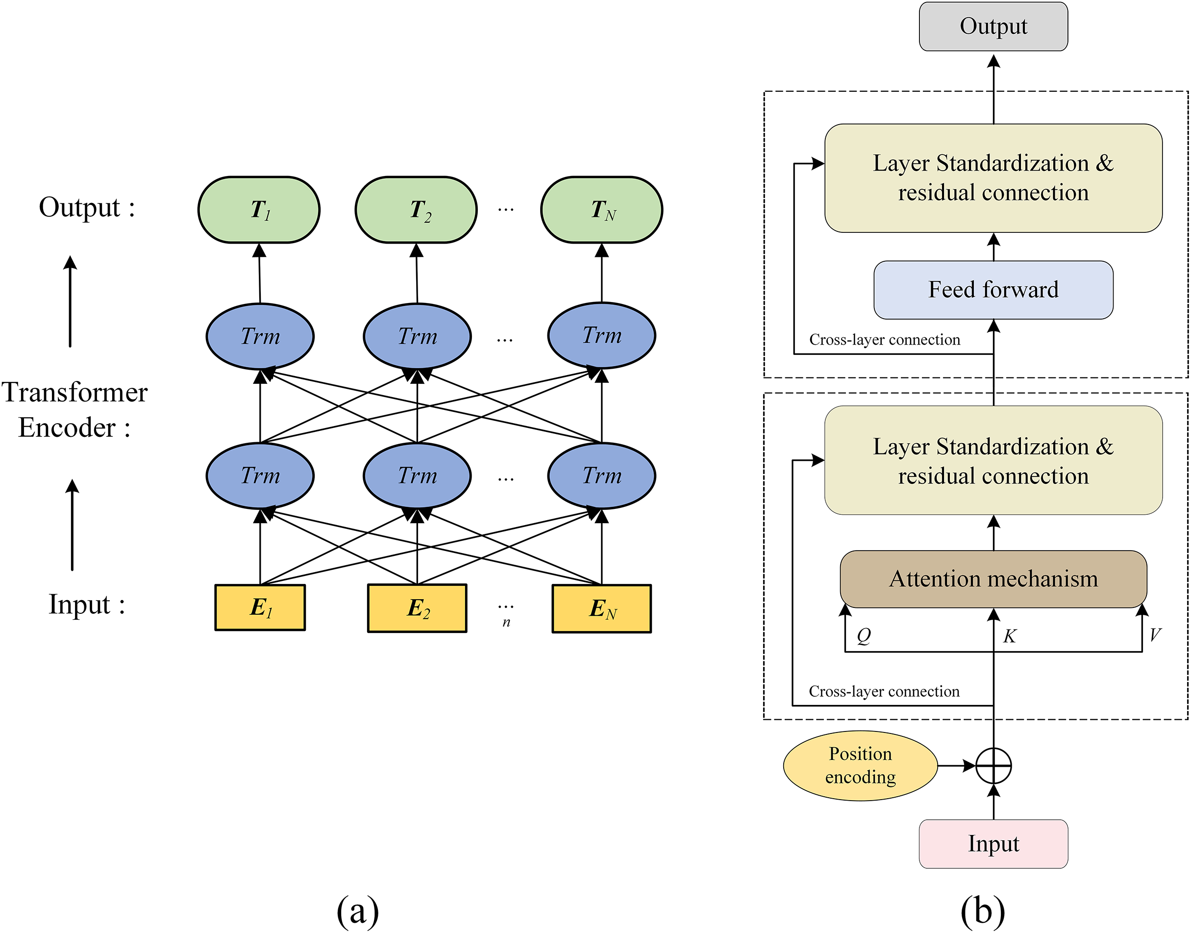
The BERT model, proposed by Google in 2018, employs a bidirectional Transformer encoder and unsupervised masked language modeling on large corpora to enhance natural language understanding and bidirectional representations (Devlin et al., 2018; Vaswani et al., 2017; Yang & Jiang, 2018). Unlike RNNs and CNNs, BERT’s attention mechanism reduces token distance to one, effectively handling long-range dependencies. For transformer defect texts, BERT accurately extracts key information such as defect type, component, and severity. Its structure is shown in Fig. 1.

Figure 1: Structure of (A) BERT model and (B) Transformer encoding structure diagram.
In Fig. 1A, the BERT feature extractor consists of four layers. The first layer (E1–En) is the embedding layer, combining token and positional embeddings to preserve semantics and order. The second and third layers are stacked Transformer encoder blocks (“Trm”) using self-attention to capture multi-level contextual dependencies for deep semantic modeling of defect texts, their structure is shown in Fig. 1B. The final layer (T1–Tn) outputs contextualized token vectors for downstream BiLSTM sequence modeling.
In Fig. 1B, the Transformer core includes a self-attention mechanism and a Feedforward Neural Network (FNN), used to extract defect text vector features. BERT’s self-attention models relationships between any two tokens, capturing semantics and internal structure. The self-attention output is computed as:
(1) where Q, K, and V are query, key, and value matrices, and dk is their dimension.
Compared with a single self-attention mechanism, multi-head attention extends this by projecting into n subspaces with distinct , and , enabling the model to focus on multiple aspects simultaneously:
(2)
(3) where Concat represents the concatenation of all hi matrices obtained from the i-th self-attention mechanism, followed by matrix multiplication with the concatenation matrix; n is the heads in the multi-head self-attention mechanism, typically set to 8; , and are the weight matrices of matrices Q, K, V in the i-th subspace.
Residual connections and layer normalization are applied after self-attention to preserve gradients, stabilize training, and improve convergence (Chen et al., 2020). The normalized output passes through an FNN with two fully connected layers, followed by another residual and normalization step, and this process is repeated. The output of the FNN model is calculated as follows:
(4) where x is the input to the feedforward neural network; w1, b1 and w2, b2 are the weights and biases of the two fully connected layers, respectively.
Theory of BiLSTM model
LSTM neural network
The LSTM neural network, proposed by Hochreiter and Schmidhuber (Jang et al., 2020; Zhou et al., 2019), enhances long-term dependency modeling by introducing three gates (input i, forget f, and output o) to control information flow within a memory cell. LSTM adapts to variable-length sequences and maintains contextual consistency, making it suitable for tasks such as Natural Language Processing (NLP), speech recognition, and time-series forecasting. Its internal structure, shown in Fig. 2A, comprises the three gates and a memory cell.
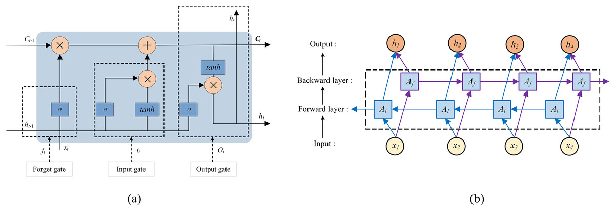
Figure 2: Structure of the (A) LSTM and (B) BiLSTM model.
The forget gate determines how much of the previous cell state is retained or discarded. As shown in Eq. (5), it processes the previous hidden state ht-1 and current input xt, outputting a value between 0 (complete discard) and 1 (full retention):
(5) where ft is the forget gate state; wf and bf are its weights and bias, and σ is the sigmoid activation function.
The input gate regulates new information entering the cell state. It evaluates ht-1 and xt, to decide which information to store, with a tanh layer generating candidate memory values. The updated cell state Ct combines retained and new information, as expressed in Eq. (6).
(6)
(7)
(8) where it is the input gate state at time step t, controlling the amount of information from xt passed to Ct; wi and bi are the weights and biases of the input gate respectively; wc and bc are the weight matrix and bias term of the cell state; tanh is the hyperbolic tangent activation function, and denotes the Hadamard product.
The output gate determines which part of the cell state is exposed as the hidden state. A sigmoid layer selects relevant cell state elements, which are then scaled by tanh to produce the output ht, also serving as the next hidden state input. The output gate is calculated as follows:
(9)
(10) where ot is the output gate state at time step t; ht-1 is the previous time step’s hidden state; wo and bo are the weight matrix and bias of the output gate, respectively.
BiLSTM neural network
Although LSTM captures long-term dependencies in sequences, it operates in a single temporal direction. BiLSTM enhances this by integrating forward and backward LSTM units, leveraging both past and future context to model long-range dependencies and richer semantic relationships (Zhou et al., 2019). As shown in Fig. 2B, forward units Af and backward units Al process the input xi, BERT-generated word vectors in this study, and their concatenated outputs hi form the extracted semantic features.
BERT generates rich contextual embeddings via transformer-based attention, yet transformer defect texts are often short, irregular, and telegraphic, which may hinder its ability to capture sequential dependencies or resolve syntactic ambiguities. To mitigate this, token embeddings from BERT’s last hidden layer are fed into a BiLSTM, producing forward and backward hidden states that are concatenated into hi for each token. This hybrid structure combines BERT’s global semantic modeling with BiLSTM’s local sequential encoding, enhancing robustness in handling ambiguous or irregular defect texts.
Defect text recognition model
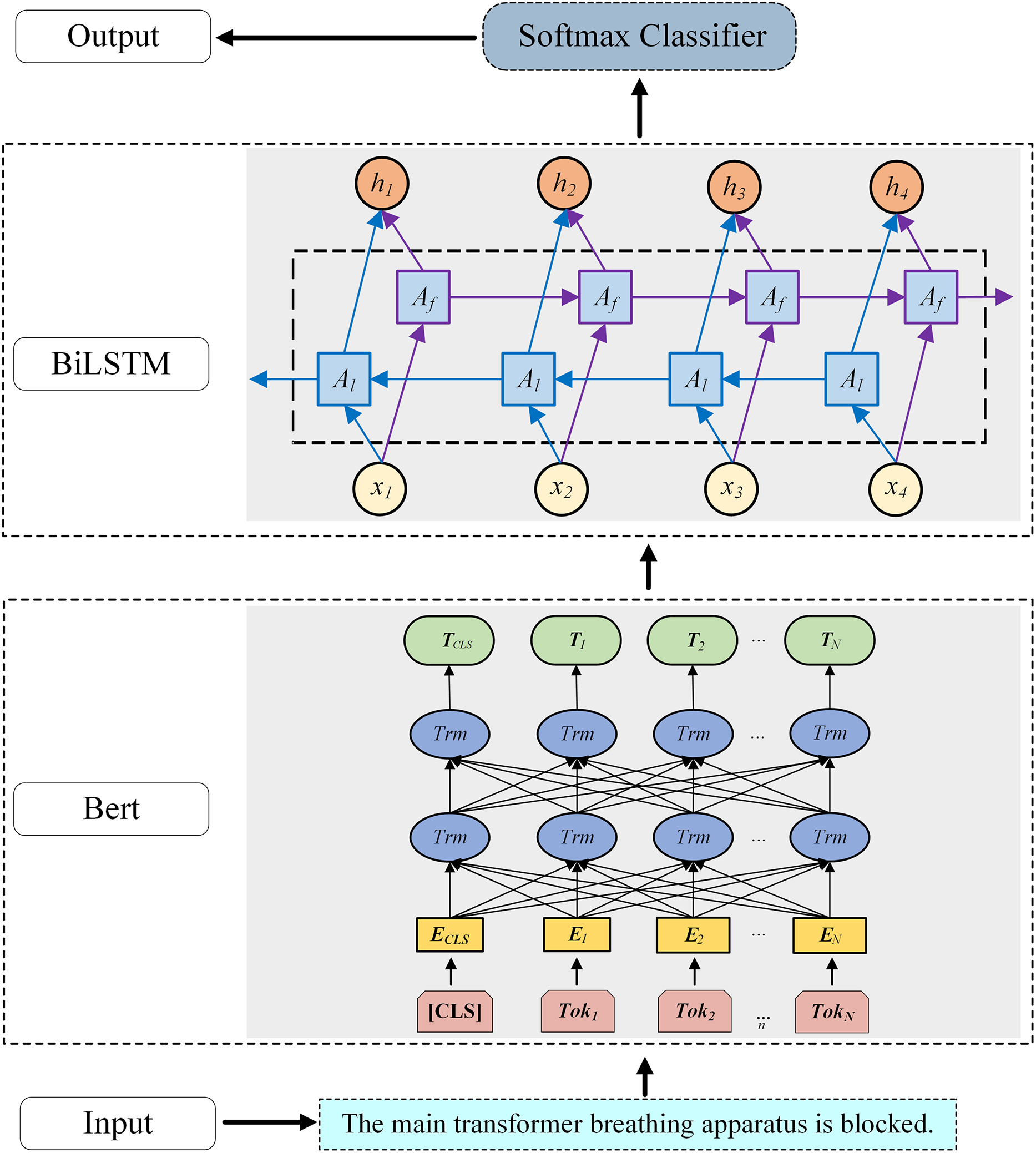
To effectively extract important features from defect texts and accurately identify defect characteristics such as performance, component, and severity in the defect texts, a defect text classification model based on BERT-BiLSTM is established, as shown in Fig. 3.
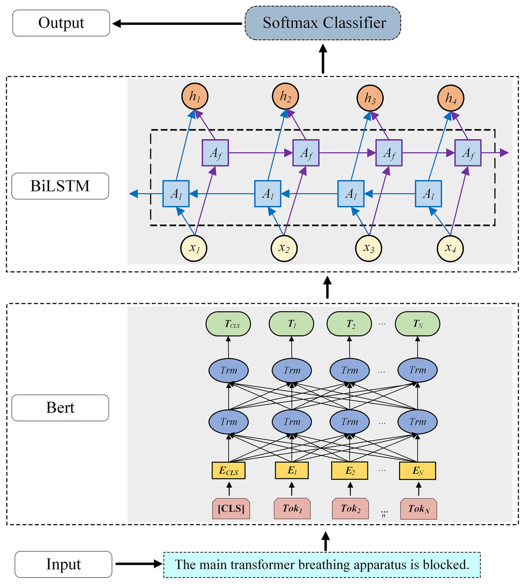
Figure 3: Structure diagram of the defect text recognition model based on BERT-BiLSTM.
First, the word embedding layer converts the input sequence into word vectors using the pre-trained BERT model. In Fig. 3, Tok1-TokN correspond to the characters or words in the defect text. The [CLS] token added at the beginning of the text represents the vector TCLS obtained after training the BERT model, which can be used for subsequent text classification. Contextual word vectors are then generated by BERT as input to the BiLSTM. Here, the Chinese BERT-Base model is used, comprising 12 transformer layers with hidden size 768, pre-trained on large-scale Chinese corpora and fine-tuned on the cleaned dataset to capture defect-domain linguistic patterns. The BiLSTM encodes forward and backward context, capturing long-range dependencies in the BERT output sequence. Finally, the decoding layer maps BiLSTM outputs to classification space via fully connected layers, and the Softmax classifier predicts defect labels.
Classification result analysis of text recognition model for transformer defect
Transformer defects text dataset setup
Based on 10,550 Alternating Current (AC) transformer defect records above 35 kV from a provincial power grid over 5 years, a defect text dataset was constructed through manual cleaning and screening. Original records, written by personnel with varying expertise, included inconsistent terminology (e.g., “main transformer” vs. “power transformer”), vague expressions (e.g., “abnormal noise” without location), and inaccurate component labels. Cleaning involved standardizing terms (e.g., unifying “cooling fan” variants), resolving ambiguities (e.g., cross-referencing components), and verifying labels (e.g., correcting severity ratings from context). After removing duplicates, errors, and invalid entries, and manually correcting missing information, 2,464 text records remained, split into training and testing sets at a 3:1 ratio. Classification labels, defect performance, component, and severity, were assigned based on the dataset and standards. The label categories and their meanings are listed in Table 2.
| Category label | Label types | Label categories | Meanings |
|---|---|---|---|
| Defect performance | 4 | Mechanical, Insulation, Thermal, Others | Types of stresses that cause defects to occur. |
| Defect component | 9 | Iron core, Winding, Oil insulation, Tank, Conservator, On-load tap-changer, Bushing, Cooling system, Non electricity protection. | The specific component or locations where defects occur. |
| Defect severity | 3 | General, Serious, Critical | The extent to which defects affect the operation of the power grid. |
The labels of each defect text in the defect text dataset are determined. The distribution of each label category in the defect dataset is shown in Fig. 4.
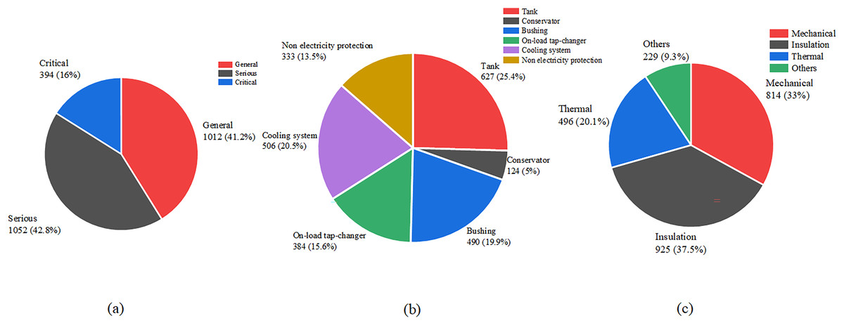
Figure 4: Label distribution of defect text datasets.
(A) Defect severity. (B) Defect component. (C) Defect type.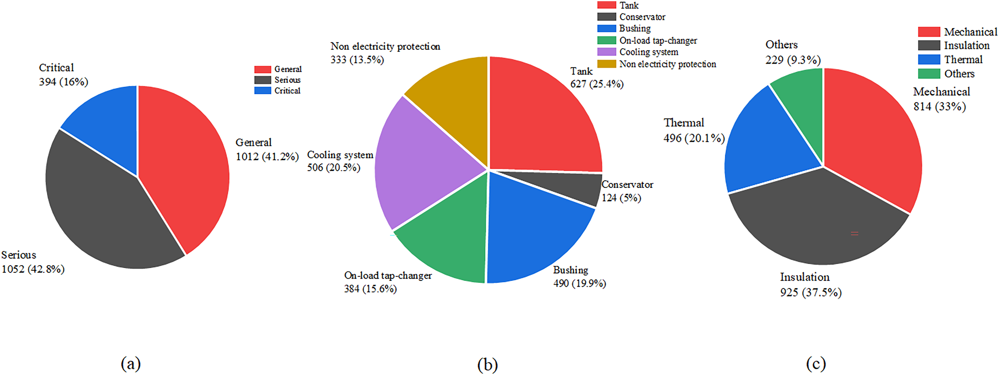
In the three label categories, sample distribution varies notably for defect severity. This due to the substantial differences in the original defect records. During routine inspections, most defects are classified as General or Serious, with few Critical cases due to low risk of major accidents. For defect components, the top five classes, tanks, cooling systems, on-load tap-changers, bushings, and non-electrical protection, have similar record counts, while defects in iron cores and windings are rare, as they are harder to detect. Regarding defect types, mechanical, insulation, and thermal defects have comparable sample sizes, whereas other types are scarce (Li & Li, 2017), consistent with expert assessments.
Classification result analysis of the BERT-BiLSTM model
This model is based on the Windows operating system and uses Python 3.7 programming language. The testing and analysis are conducted based on the TensorFlow deep learning framework and the Keras neural network framework. The key parameters of the model are selected, as shown in Table 3.
| Parameter | Value |
|---|---|
| Hidden_size | 768 |
| Batch_size | 128 |
| Dropout | 0.5 |
| Activation function | ReLU |
| Forward hidden_size | 384 |
| Backward hidden_size | 384 |
| Learning_rate | 5 × 10⁻⁵ |
| Optimizer | Adam |
| Num_epochs | 30 |
| Word vector dimension | 128 |
Hyperparameters were determined via empirical tuning and transformer text classification studies. A learning rate of 5 × 10⁻⁵ and batch size of 128 ensured stable convergence. To mitigate overfitting on the moderate, noisy dataset, a dropout layer (0.5) followed the BiLSTM, with early stopping applied based on validation loss. Hidden layer size balanced expressiveness and computation, and 30 epochs sufficed for convergence. Rectified Linear Unit (ReLU) activation and Adam optimizer were used, with Adam adaptively minimizing loss.
To address class imbalance, class weights—set inversely proportional to class frequency—were incorporated into the loss function,increasing the gradient impact of minority classes and reducing bias toward majority classes without resampling or architectural changes.
Effective text classification is an important module for assessing the performance of text recognition models. In this article, model performance is evaluated using precision, recall, F1-score, accuracy, and the confusion matrix, defined as follows:
(11)
(12)
(13)
(14) where TP, TN, FP, and FN correspond to the numbers of true positives case, true negatives case, false positives case, and false negatives case, respectively.
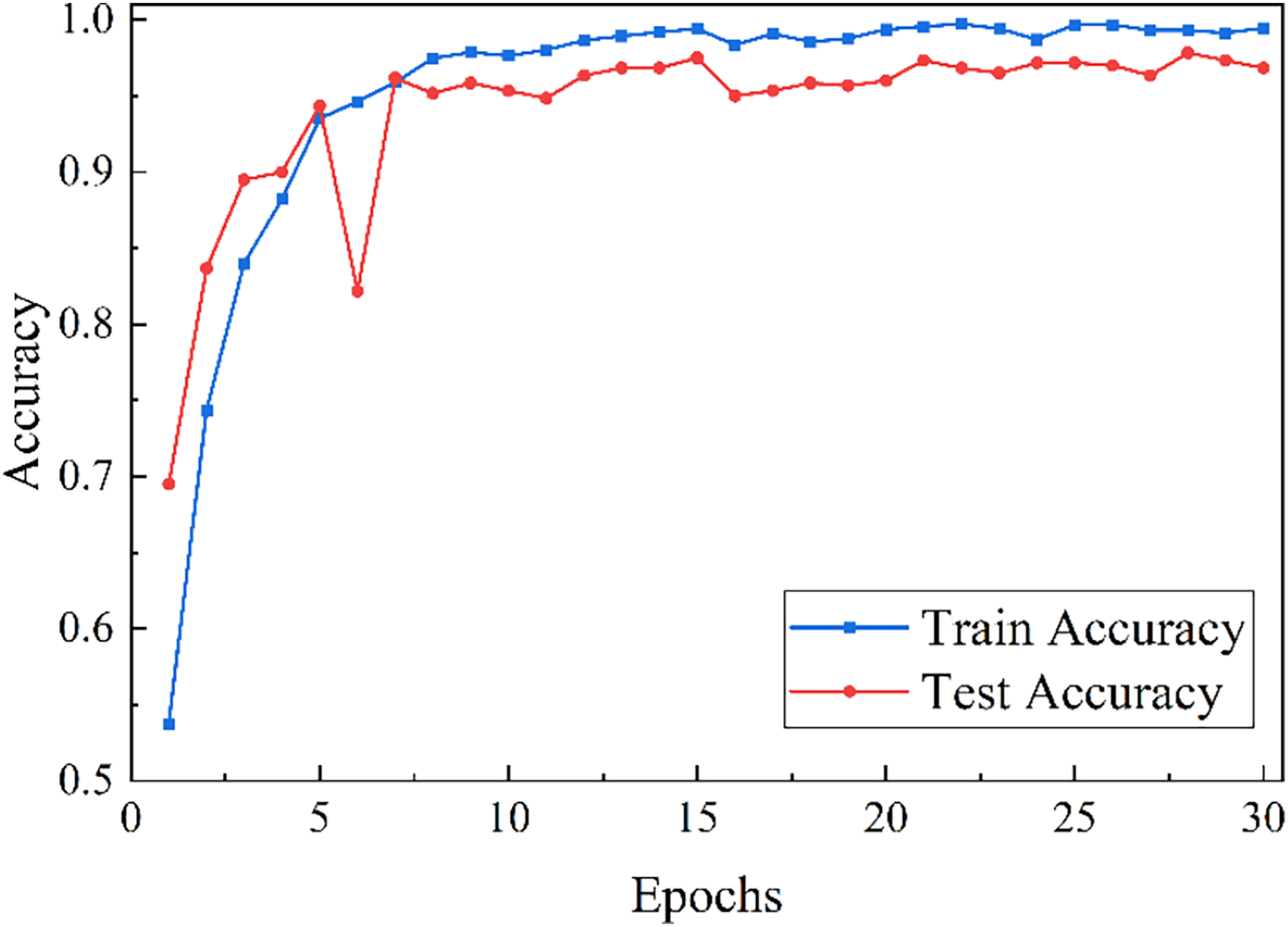
Taking defect severity classification as an example, Fig. 5 presents the model’s performance on the training and testing sets. Although fluctuations occur during training, accuracy and loss gradually converge with increasing epochs, stabilizing around epoch 18. At 30 epochs, the model achieves an accuracy of 96.83%.
Figure 5: Trend of model classification accuracy and loss.
The evaluation results of the BERT-BiLSTM model for the three defect text classification tasks are shown in Table 4. The model achieves over 94% accuracy for defect severity and defect component classification, while defect type classification attains a comparatively lower accuracy of over 84%.
| Label type | Precision | Recall | F1-score | Accuracy |
|---|---|---|---|---|
| Defect severity | 0.968 | 0.970 | 0.969 | 0.970 |
| Defect component | 0.948 | 0.947 | 0.945 | 0.947 |
| Defect performance | 0.845 | 0.848 | 0.846 | 0.848 |
The confusion matrix results for the three types of text classification problems are shown in Fig. 6. The BERT-BiLSTM model has good performance in defect severity and component classification, but low in defect type recognition.
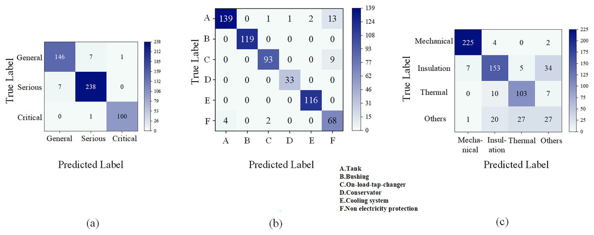
Figure 6: Confusion matrix of the classification models.
(A) Defect severity. (B) Defect component. (C) Defect type.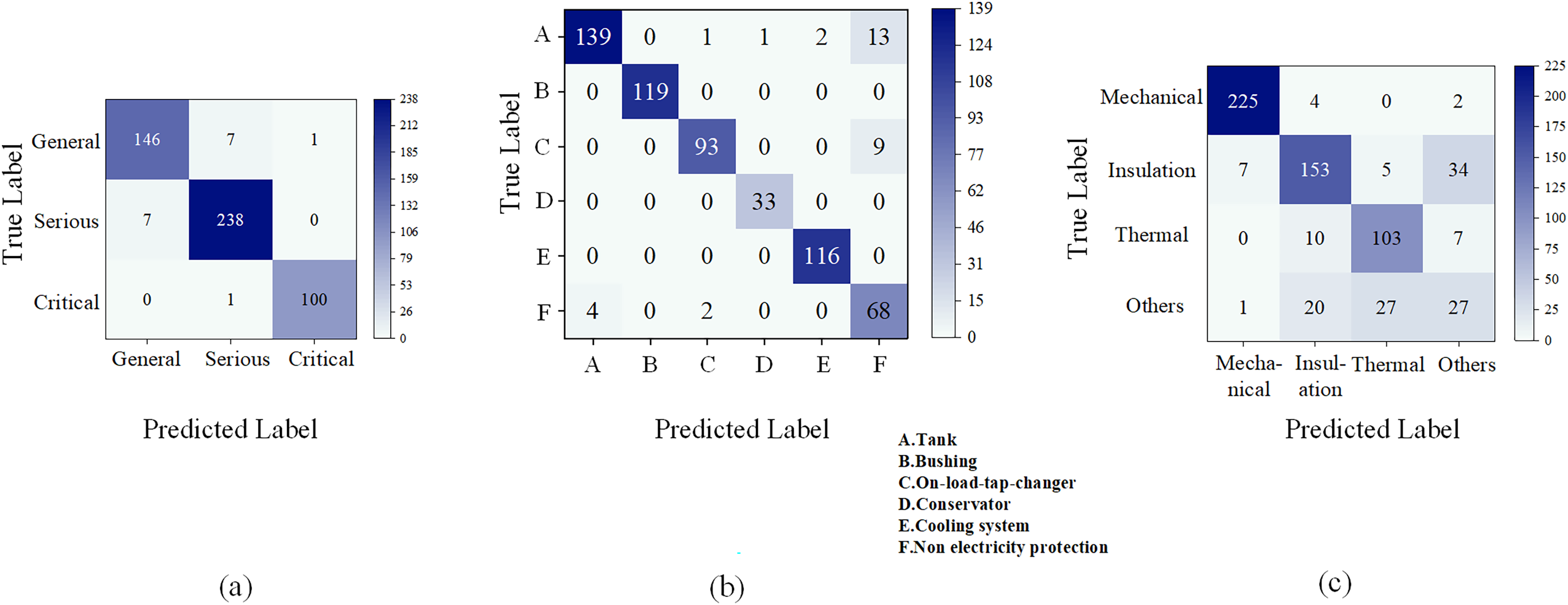
Misclassification of defect severity mainly arises between general and severe levels due to vague descriptions. Component errors frequently occur among tank, conservator, and non-electrical protection devices when multiple components are mentioned ambiguously. Defect type classification is hindered by sample imbalance and fuzzy semantic boundaries, particularly between mechanical and thermal faults. Many “other” defects, such as auxiliary system issues, share textual features with overheating or insulation faults, leading to misclassification. Moreover, independent category prediction in the BERT-BiLSTM model neglects correlations between defect type and component, reducing classification accuracy.
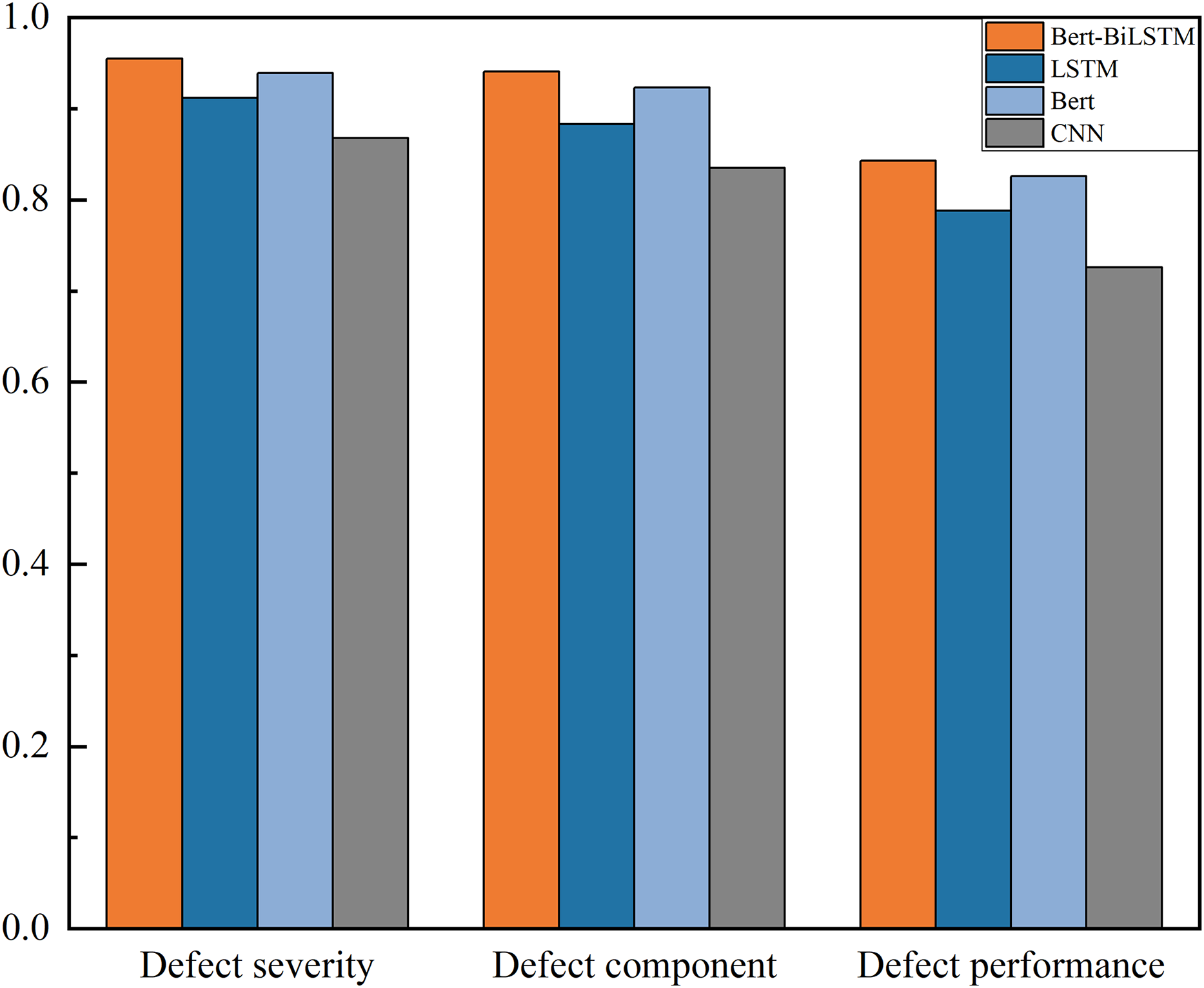
Comparison with general classification models
Based on the above evaluation metrics, the effectiveness of the BERT-BiLSTM model and commonly used text classification models such as CNN, BERT, and LSTM are compared, as shown in Fig. 7.
Figure 7: Comparison of model effects under different text classification problems.
The results show that the evaluation metric distribution across the three classification tasks is consistent with other models, but BERT-BiLSTM achieves the highest F1-score (>84%), 2–5% higher than alternatives, indicating superior semantic extraction for transformer defect texts. The F1-score ranking is BERT-BiLSTM > BERT > LSTM > CNN. The reasons may be: (1) LSTM alone outperforms BERT, suggesting that while LSTM efficiently mines defect text features, its global feature extraction contains noise that BERT’s bidirectional encoding can mitigate. (2) CNN performs worst, particularly with long texts, due to its shallow sequential feature extraction and inability to capture deep semantic context.
In addition to classification performance, the computational efficiency and resource demands of the four models are shown in Table 5. The BERT-BiLSTM model has the longest training time (1 h 13 min for 30 epochs), the largest parameter count (~113.5 M), and peak GPU usage (~6.3 GB) due to its dual-layer architecture. Once trained, inference is efficient, taking only a few hundred milliseconds per sample. By contrast, CNN and LSTM consume fewer resources but capture complex semantic dependencies less effectively, leading to lower classification accuracy, highlighting the advantage of BERT-BiLSTM for tasks requiring precise diagnostics.
| Models | Training times (30 epochs) |
Parameters (Million) | Peak GPU memory usage |
|---|---|---|---|
| CNN | 45 min | ~2.1 M | ~1.2 GB |
| LSTM | 58 min | ~5.4 M | ~1.8 GB |
| BERT | 1 h 05 min | ~110 M | ~4.5 GB |
| BERT-BiLSTM | 1 h 13 min | ~113.5 M | ~5.3 GB |
Condition assessment of power transformer
Transformer condition assessment
Transformer condition assessment, fundamental for equipment maintenance decision-making, evaluates equipment health based on operation, maintenance, and testing. Condition maintenance uses these assessments to determine operational status and guide maintenance plans. Results are expressed as condition scores (quantitative) and grades (qualitative), which correspond to each other, though grade assignment may vary across standards or procedures.
In transformer health management systems, condition assessment often depends on online monitoring data, offline diagnostic test results, and analysis of feature quantities such as dissolved gases to evaluate the health status of the transformer. However, the influence of historical defect events (recorded as unstructured textual descriptions) on equipment condition should not be neglected. Despite their availability, these records are rarelyu sed as direct inputs of health assessment models.
To address this gap, an assessment method that integrates defect text recognition with transformer condition evaluation is proposed, as shown in Fig. 8.
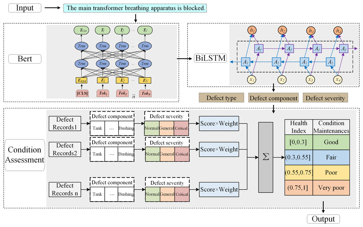
Figure 8: Framework of the assessment method.
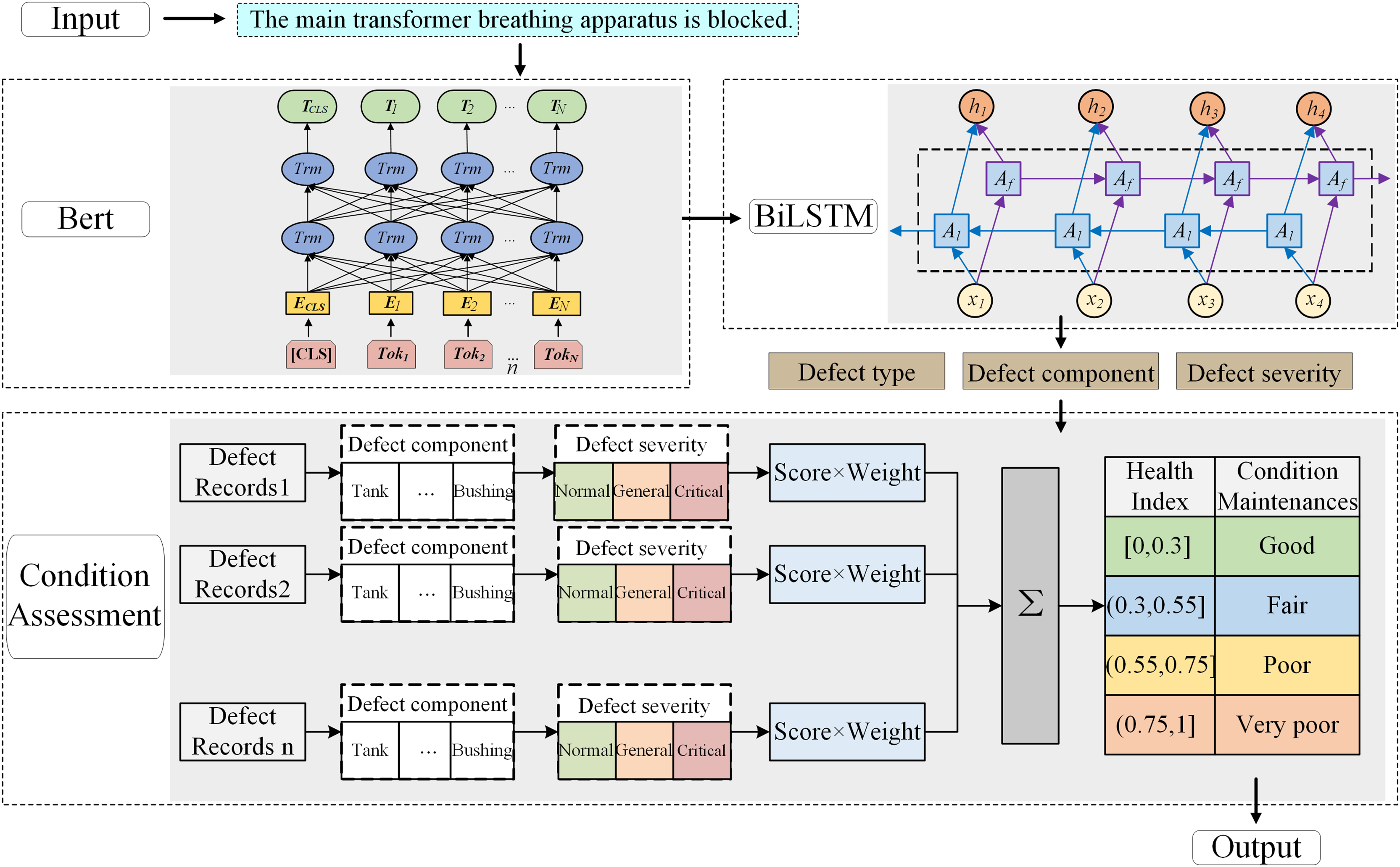
This method first uses a BERT BiLSTM classification model to extract defect-related information (such as defect type, component, and severity). Then, according to the national transformer health assessment standards, these features are mapped to structured evaluation criteria, enabling automatic generation of condition scores and grades based on defect history. This framework cannot only broaden the data sources used in condition evaluation, but also support intelligent fault triage and maintenance decision-making in scenarios where sensor data may be unavailable or insufficient.
Association rules for status evaluation
In actual work, based on the understanding of equipment principles and operating conditions, a reasonable equipment defect classification method can be formulated. Considering the internal structure of the equipment, external environment, and operating conditions, combined with the actual status of the equipment, the defect rating score for power transformer and the weighting of defect status score are shown in Table 6.
| Defect rating | Defect status | Transformer condition maintenance | ||||
|---|---|---|---|---|---|---|
| Equipment defects | Grade interval (k) | Condition | Weight (wi) | Equipment condition | Health index | Condition maintenances |
| Normal | 0 | Tank | 0.3 | Good | [0, 0.3] | Normal maintenance or extension for 1 year. |
| General | 4 | Conservator | 0.1 | Fair | (0.3, 0.55] | Appropriate reduction of maintenance cycles |
| Serious | 8 | Bushing | 0.22 | Poor | (0.55, 0.75] | Schedule maintance in due course. |
| Critical | 12 | Cooling system | 0.12 | Very poor | (0.75, 1] | Immediately arrange maintenance. |
| On-load tap-changer | 0.18 | |||||
| Non electricity protection | 0.08 | |||||
In this framework, the BERT-BiLSTM model’s classification outputs—defect severity, component, and performance—serve as inputs to the scoring system. Predicted severity levels are mapped to score deductions (Table 5), and component types are assigned weights (Table 6). Label definitions and scoring thresholds follow national standards (e.g., DL/T 572, Q/GDW 11247) and are validated by maintenance experts.
Component weights reflect criticality and operational risk, determined via expert judgment and historical fault analysis. An adaptive correction mechanism dynamically adjusts health scores based on abnormal operation indicators, improving contextual accuracy. Expert validation indicates this approach better reflects operational risks than fixed weights, although formal ablation studies were not conducted.
According to the above condition evaluation rules, the deduction points of its transformer equipment are obtained, corresponding to the health status. Maintenance strategies can be developed based on the results of health index. The health index is calculated as follows:
(15)
(16) where a and k are respectively the number and score of different defect classes; ni represents the overall score of the component; wi represents the weight of the component, as shown in Table 6, and m represents the total number of classifications of defect component.
In traditional state evaluation, indicator weights remain fixed once determined. However, when an indicator exceeds normal values, its abnormal information may be underestimated due to a small original weight, which is impractical. To address this, a dynamic weight calculation with adaptive correction is employed. When an indicator shows a high state value, its importance in accurately assessing the current equipment health increases, making it a key factor in the comprehensive evaluation. Its weight is appropriately adjusted to reflect its critical impact on transformer condition. When n indicators exceed abnormal thresholds, they are recorded as set A, while m normal indicators form set B. The weights of the abnormal indicators are then adjusted as follows:
(17)
The remaining normal indicators are adjusted as follows:
(18)
(19)
Using the above scoring rules, the impact of historical defects on a transformer can be assessed to determine its health status and guide appropriate maintenance strategies. According to oil-immersed transformer condition evaluation guidelines, transformer status is categorized into four levels: good, fair, poor, and very poor. The corresponding maintenance programs for each status are listed in Table 6.
Case study
To verify the applicability of the proposed method for transformer condition assessment, we selected a real case involving a 35 kV AC transformer with multiple recorded defect events in the past year. The specific defect instances and their corresponding classification results are shown in Table 7.
| Transformer | Defect text | Defect severity | Defect condition | Health index | Equipment condition |
|---|---|---|---|---|---|
| A 35kV AC transformer | [Transformer, cooling system, air-cooled] Failure of a single fan. | General k = 4 |
cooling system wi = 0.12 |
HI = 0.44 | Fair |
| [Transformer, oil-immersed transformer, tank] Oil leakage was detected from the transformer tank at a rate of approximately one drop per minute. | General k = 4 |
tank wi = 0.3 |
|||
| The temperature of the B-phase bushing of the transformer reached 55.2 degrees. | Serious k = 8 |
Bushing wi = 0.22 |
Appropriate reduction of maintenance cycles | ||
| Smoking occurred in the transformer tank. | Critical k = 12 |
Tank wi = 0.3 |
Each defect text in Table 7 was processed by the BERT-BiLSTM model to extract three core elements: defect severity, component, and type. Component weights (wi) were assigned based on a predefined expert knowledge base, and severity levels (ki) were quantified via mapping rules. The overall Health Index (HI) was calculated using Eqs. (16) and (17), with a weighted aggregation across components. An HI of 0.44 corresponds to the “Fair” condition zone in Table 6, indicating moderate degradation. Although a critical defect (e.g., oil tank smoke) exists, its impact is offset by less severe defects and component weights. The recommended maintenance strategy is to shorten inspection intervals and perform targeted fault tracing, particularly for the tank and cooling system.
This case demonstrates the feasibility and effectiveness of the proposed framework and highlights the potential of NLP-based methods in digital power equipment management.
Conclusion
In intelligent power systems, natural language processing and deep learning are employed to classify defect texts. For transformer equipment, this approach can significantly accelerate fault diagnosis and localization by maintenance personnel, reduce maintenance costs and workload, support scientific maintenance decision-making, and provide essential evidence for assessing current equipment health.
A transformer defect text recognition model based on BERT-BiLSTM was proposed. It can identify features of the severity level, component, and type of equipment defects based on defect texts. The results indicate that the model can achieves an accuracy of more than 94% in identifying the defect severity and defect component. Comparative experiments further validate that the F1-score of the text classification model is more than 2% higher than that of models such as BERT, CNN and LSTM.
After adopting text recognition methods, health assessment rules are determined based on the relevant state assessment guidelines and standards for transformers by evaluating the status of defective equipment. After conducting health indicator evaluation calculations, the healthy operating status of the equipment can be obtained, and reasonable arrangements can be made based on this. The maintenance plan can effectively optimize the allocation of transportation and inspection resources.
Although the proposed approach demonstrates robust performance in defect classification and condition assessment, its generalization may be affected by variability in real-world input. Future work will optimize the model architecture, incorporate correlations between defect locations and types, and integrate real-time operational data, such as sensor measurements, to enhance diagnostic accuracy and temporal responsiveness. The methodology will be deployed in intelligent maintenance decision support systems and validated through on-site applications and expert feedback.