
The Silhouette coefficient and the Davies-Bouldin index are more informative than Dunn index, Calinski-Harabasz index, Shannon entropy, and Gap statistic for unsupervised clustering internal evaluation of two convex clusters
- Published
- Accepted
- Received
- Academic Editor
- Marco Piangerelli
- Subject Areas
- Algorithms and Analysis of Algorithms, Artificial Intelligence, Data Mining and Machine Learning, Data Science, Databases
- Keywords
- Clustering, Clustering internal metrics, Silhouette coefficient, Shannon entropy, Davies-Bouldin index, Dunn index, Calinski-Harabasz index, Gap statistic
- Copyright
- © 2025 Chicco et al.
- Licence
- This is an open access article distributed under the terms of the Creative Commons Attribution License, which permits unrestricted use, distribution, reproduction and adaptation in any medium and for any purpose provided that it is properly attributed. For attribution, the original author(s), title, publication source (PeerJ Computer Science) and either DOI or URL of the article must be cited.
- Cite this article
- 2025. The Silhouette coefficient and the Davies-Bouldin index are more informative than Dunn index, Calinski-Harabasz index, Shannon entropy, and Gap statistic for unsupervised clustering internal evaluation of two convex clusters. PeerJ Computer Science 11:e3309 https://doi.org/10.7717/peerj-cs.3309
Abstract
Clustering is an area of unsupervised machine learning where a computational algorithm groups together similar points into clusters in a meaningful way, according to the algorithm’s properties. When external ground truth for the clustering results assessment is available, researchers can employ an external clustering assessment metrics and evaluate the quality of the clustering results this way. When no external gold standard is available, however, researchers need to use metrics for internal clustering assessment, which produce an outcome just considering the internal data points of the clusters identified. Although consensus regarding the usage of the adjusted Rand index for the external clustering assessment exists, there is no standard regarding internal metrics. We fill this gap by presenting this study on comparing the six internal metrics clustering most commonly used in bioinformatics and health informatics: Silhouette coefficient, Davies-Bouldin index, Dunn index, Calinski-Harabasz index, Shannon entropy, and Gap statistic. We first analyze their mathematical properties, and then test them on the results of k-means with k = 2 clusters on multiple different convex-shaped artificial datasets and on five real-world open medical datasets of electronic health records. Our results show that the Silhouette coefficient and the Davies-Bouldin index are more informative and reliable than the other analyzed rates, when assessing convex-shaped and non-nested clusters in the Euclidean space.
Introduction
The problem: Machine learning methods can be categorized into two groups: supervised and unsupervised techniques. When the ground truth or the gold standard regarding a scientific dataset is available, one can use that information to improve their computational algorithm: these problems are called supervised. On the contrary, when no real-world truth regarding a dataset is available, one can try to partition the dataset into different groups of points, and see if these divisions lead to meaningful groups: these problems are called unsupervised, and the unsupervised techniques that group data are called clustering. When a clustering analysis is performed, however, it is difficult to state if the quality of its results is good or bad. To this end, metrics such as Silhouette coefficient, Davies-Bouldin index (DBI), Calinski-Harabasz index (CHI), Dunn index, Shannon entropy, and Gap statistic can be employed without the need of having an external ground truth. These metrics provide an indication of the geometrical properties of the discovered clusters, such as their separation or compactness, providing a measure of quality corresponding to some intuitive definition of what a good clustering is.
All these metrics, although useful, have advantages and limitations. For this reason, no consensus regarding a single one to use in all cases has been reached in the scientific community. We fill this gap by presenting the current study, where we studied the six mentioned metrics and applied them to the results of -means on convex-shaped artificial datasets and real-world medical data, by using a data science approach. We decided to focus on -means because it is one of the most popular clustering algorithms (Ashabi, Sahibuddin & Haghighi, 2020) ( -means is mentioned by more than two million scientific articles on Google Scholar today: way more than any other clustering method).
Given the enormous generalizability of this problem, we focused on the convex-shaped clusters, and do not consider nested, concave-shaped clusters (that might be found by density-based clustering algorithms such as Density-Based Spatial Clustering of Applications with Noise (DBSCAN) to be clear) in this study. We tested these six coefficients on the -means clusters obtained first on artificial datasets and then on real-world biomedical datasets, and analyzed their behavior. Our results show clearly that Silhouette coefficient and Davies-Bouldin index resulted being more reliable and trustworthy than the other rates, with the Silhouette coefficient having the advantage to produce results only in a closed interval, and the DBI having the advantage to generate consistent results when the clustering results are bad.
Literature review: Several studies proposed theoretical and statistical comparison between metrics, to establish which rate could be more informative. Arbelaitz et al. (2013) and Gurrutxaga et al. (2011) employed thirty different metrics, including the Dunn index, Calinski-Harabasz index (CHI), Davies-Bouldin index (DBI), and Silhouette coefficient to verify the effectiveness of these metrics on five tasks: number of clusters, dimensionality, cluster overlap, cluster density, and noise level. The author of this study claimed that Silhouette coefficient obtained the best results many of the tests they performed, but their aim was to identify the “best” number of clusters according to a presumed “correct” number of clusters.
The study of Lamirel (2016) described a comparison between the Dunn index, Davies-Bouldin index, Silhouette coefficient, Calinski-Harabasz index, and the Xie-Beni index, where he applied clustering algorithms to datasets where the optimal number of clusters is known in advance. The author claimed the current existing metric for internal clustering evaluation are unsatisfactory, and proposed a new index based on feature maximization.
Gagolewski, Bartoszuk & Cena (2021), in their project, employed several different metrics for internal clustering assessment, including the Silhouette coefficient, Davies-Bouldin index, Calinski-Harabasz index and Dunn index. They applied these metrics on the results of several clustering algorithms, including -means, and then verified their validity by employing experts’ knowledge: they used labels annotated to the data points by experts, and compared them with the labels assigned by the clustering algorithms. In the end, the authors proposed a new variant of the Dunn index, based on ordered weighted averaging operators, as most informative metric. Gagolewski, Bartoszuk & Cena (2021) utilized the scikit-learn Python package, too.
In their study, Oztürk & Demirel (2023) showed a comparison between the Silhouette coefficient, Caliński-Harabasz index, Davies-Bouldin index, and Dunn index applied to the results of -means when the goal is to determine the best number of clusters. To assess the effectiveness of their approach, they used datasets where the presumed optimal number of clusters was already known.
Finding the best number of clusters is also the main goal of the study by Baarsch & Celebi (2012): they utilized several metrics (including Dunn, Davies-Bouldin, Calinski-Harabasz, and Silhouette) calculated on the results of -means. They employed synthetic datasets where the “right” number of partitions was clearly visible, and used that as ground truth.
Also, Maulik & Bandyopadhyay (2002) used several internal clustering metrics to assess the “best” number of clusters. They applied -means on datasets downloaded from the University of California Irvine Machine Learning Repository (University of California Irvine, 1987) where the supposed optimal number of cluster was already available, and they checked which internal metric identified that “correct” number. Afterwards, they applied the simulated annealing algorithm to the dataset to properly partition the data into those clusters.
Liu et al. (2010) assessed multiple metrics for internal clustering assessment by taking into account two aspects: compactness (how close points of a cluster are) and separation (how well separated is a cluster from the others). They then applied these metrics on the results of -means on synthetic datasets designed to consider five properties: monotonicity, noise, density, subclusters, and skewed distributions. Their study claims that the S_Dbw (Halkidi & Vazirgiannis, 2001) resulted being the only metric that performed well for all the five properties.
-means was also employed in the study by Shim, Chung & Choi (2005), which then measured the results through the Calinski-Harabasz index, Davies-Bouldin index, and other twelve metrics. These researchers used datasets of points with already known partitions, and then stated which metric was consistent with the already-known information.
The study of Petrovic (2006) utilized the Silhouette coefficient and Davies-Bouldin index to assess the clustering results of a computational intrusion detection system, which are security tools designed to detect and classify attacks against computer networks and host (Petrovic, 2006). He calculated these metrics on the results of -means with clusters, and eventually claimed that the Silhouette coefficient produced more accurate results than DBI.
Differently from the just-described studies, Soni & Choubey (2014), applied the hierarchical clustering algorithm, and not -means, to the LIBRA dataset found on the UC Irvine ML Repo (University of California Irvine, 1987). They used this method by reducing the feature space at multiple times, and then measured the results through the Calinski-Harabasz index, Dunn index, Davies-Bouldin index, and Silhouette index, stating that CHI outperformed all the other rates.
Lastly, José-García & Gómeaz-Flores (2021) presented a detailed survey on twenty-two metrics for internal clustering, including Silhouette coefficient, Calinski-Harabasz index, Dunn index, Davies-Bouldin index, and others. They utilized an evolutionary clustering algorithm on several real-world and synthetic datasets, having different properties (linearly separable datasets having well-separated clusters, linearly separable data having overlapped clusters, non-linearly separable data having arbitrarily-shaped clusters, and real-world life datasets) having already-known cluster number (José-García & Gómeaz-Flores, 2021). The authors then employed the Adjusted Rand Index (ARI) (like we do in our present study), and the normalized absolute error to assess the clustering results, and compare them with the results of the twenty-two analyzed metrics. Their results showed that Silhouette coefficient achieved the most reliable outcomes, followed by the Calinski-Harabasz index. This survey also states that all the studied metrics “performed poorly in non-linearly separable data with arbitrary cluster shapes” (José-García & Gómeaz-Flores, 2021), suggesting room for improvement in the unsupervised machine learning community.
Some studies employed the indices for internal clustering assessment to solve a specific scientific problem, and not to try find the most informative metric. This is the case of Bolshakova & Azuaje (2003), which utilized several metrics on gene expression data, in particular to detect the most proper number of clusters in that context. These authors did not make a claim on a specific metric outperforming the others.
Another application study is the article by Ashari et al. (2023), where the authors employed several clustering indices on the clustering results of data of floods in Jakarta, without claiming the superiority of one index on the others.
Other studies investigated the validity of clustering internal indices, by observing which of them found the “correct” number of clusters in several cluster analysis applications. This is the case of Todeschini et al. (2024), Akhanli & Hennig (2020), and Niemelä, Äyrämö & Kärkkäinen (2018). The issue with these studies is that they announced a “correct” number of clusters for each specific dataset analyzed beforehand, and then checked which of the studied internal metric identified that number as best . Similarly, Liu et al. (2012) applied several clustering metrics together with particle swarm optimization (PSO). Several studies by Christian Hennig, moreover, provide some guidelines on the choice of clustering evaluation coefficients (Hennig, 2007, 2015; Hennig et al., 2015).
Even if these studies offer interesting comparisons between internal clustering coefficients, they all suffer from the same flaw: their authors employ several internal clustering indices and various clustering algorithms to find the “best” or “correct” number of clusters. The identification of the “best” or “correct” number of clusters is, in fact, one of the main scientific research questions in computational statistics and unsupervised machine learning. To give you an idea, the query “number of clusters optimization” on Google Scholar today yields around 4.6 million articles.
Unlike these studies, we decided not to frame the scientific question of which clustering internal index is more informative into the “best k” problem. In our tests on artificial data, in fact, we decided to set the number of clusters to two beforehand, and improved or worsened the cluster composition of the data to see which internal metrics would improve or worsen as well: we can say that our rationale is to understand which clustering internal indices confirm the clustering results trends or not.
Our study: In this project, we analyzed six different metrics for the same scope by choosing the ones that are most common in bioinformatics and health informatics studies: Silhouette coefficient, Davies-Bouldin index, Calinski-Harabasz index, Dunn index, Shannon entropy, and Gap statistic. Our tests demonstrate that the Davies-Bouldin index and the Silhouette coefficient are the most reliable internal metric for the assessments of convex-shaped clustering results obtained through -means with k = 2 clusters, among the six coefficients studied here, both in the tests made on artificial datasets and in the tests made on real-world electronic health record (EHR) datasets. Moreover, we also performed tests on artificial public datasets having a “right” number of clusters, and these two coefficients obtained reliable results in those cases, too.
We organize the rest of the article as follows. After this Introduction, we introduce the six metrics, their formulas and their mathematical properties in ‘Metrics and Mathematical Backgrounds’. We then describe the tests we did by using these metrics on the results of -means on artificial data and on real-world medical data in ‘Results’. Eventually, we report a detailed discussion about the results and outline some conclusions in ‘Discussion and Conclusions’.
Metrics and mathematical backgrounds
In this section, we outline and describe the six metrics for internal clustering assessment analyzed in this article. We also summarize their possible values in Table 1.
| Metric | Interval | Meaning |
|---|---|---|
| Silhouette coefficient (Rousseeuw, 1987) | The higher, the better | |
| Shannon entropy (Shannon, 1948) | [0; ] | The lower, the better |
| Davies-Bouldin index (Davies & Bouldin, 1979) | [0; ) | The lower, the better |
| Dunn index (Dunn, 1974) | [0; ) | The higher, the better |
| Calinski-Harabasz index (Calinski & Harabasz, 1974) | [0; ) | The higher, the better |
| Gap statistic (Tibshirani, Walther & Hastie, 2001) | ( ; ) | The higher, the better |
Silhouette coefficient
The Silhouette metric is the more famous and widespread method for evaluating and validating clustering consistency. Introduced by Peter J. Rousseeuw in 1986 (Rousseeuw, 1987), its rationale consists in employing a natural and straightforward procedure to assess the relation between inter-cluster and intra-cluster mutual distances between points. As such, the Silhouette formula is a functional, defined for each point of the dataset, having also the chosen distance as an hyperparameter, with the Euclidean often chosen as the default in several implementations. However, different distances such as Manhattan will lead to different numerical outcomes for the final score. In detail, for a chosen distance function and for a dataset partitioned in clusters , given a data point belonging to a non-singleton cluster , define
as the intra-cluster dissimilarity measure, and
as the intercluster dissimilarity measure and
(1) as the Silhouette score; for a single point cluster , set .
The Silhouette score ranges from –1 (worst and minimal value) to +1 (best and maximum value) (Table 1).
Shannon entropy
Shannon entropy (Shannon, 1948; SciPy, 2025; Meilǎ, 2007), also known as information entropy and derived from information theory, is a measure that quantifies the uncertainty associated with a probability distribution. In clustering quality assessment, Shannon entropy is used to measure how well clusters separate data. A low value of entropy indicates that the data are well separated into clusters, suggesting that the clustering is of good quality. A high value of entropy, on the other hand, indicates that the data are more evenly distributed among the clusters, suggesting that the clustering may not be effective in separating the data into distinct groups. To calculate the Shannon entropy for a clustering result, the following steps are taken:
-
1.
Assignment of the data to the clusters: Let us suppose we have clusters and data point. Every data point is assigned to the cluster by some method.
-
2.
Probability distribution: We calculate the proportion of data in each cluster. The probability that a data point belongs to the cluster is given by: where is the number of data points within the cluster and is the total number of data points.
-
3.
Calculation of the Shannon entropy: We finally calculate the Shannon entropy H for this clustering by using this formula: (2)
Shannon entropy possible values range from 0 (minimal and perfect value) to (maximum and worst possible value) (Table 1). If we have clusters, Shannon entropy ranges from 0 to 1.
To have a scenario where values of the metric increases when results get better, we decided to use the complementary Shannon entropy, defined as . The complementary Shannon entropy with ranges from 0 to 1, where 0 is the worst possible outcome and 1 is the best possible outcome.
Davies-Bouldin index
The Davies-Bouldin index or ratio (Davies & Bouldin, 1979) represents the ratio of the sum of the within-cluster dispersion to the between-cluster separation. Compared with the Silhouette coefficient, the Davies-Bouldin index does not have a limited range of values; rather it can take any value greater than or equal to 0. The closer the value is to 0 the higher the clustering quality, consequently the larger the value the lower the clustering quality.
The formula is the following:
(3) where:
and
with:
where is a data point of the cluster, is the centroid of the cluster, and is the number of data points in the cluster. Thus represents the dispersion of the cluster. is the distance between the two centroids.
The DBI ranges from 0 (minimal and perfect outcome) to infinity (maximum and worst outcome possible) (Table 1). Since all the other metrics have low values for bad results and high values for good results, we decided to use reciprocal DBI = 1/DBI. The interval of reciprocal DBI is (0; ), the higher the value the better the result.
Dunn index
The Dunn index (DI) (Dunn, 1974) is an index that measures the degree of compactness of clusters and the degree of separation between clusters. Dunn index does not have a limited range of values, but rather can take any value greater than or equal to 0. The more the value tends to infinity the higher the cluster quality will be; and consequently the smaller the value the lower the clustering quality will be. The formula for the Dunn index is as follows:
where:
is the distance between the cluster and the cluster. This distance can be defined in several ways, for example as the minimal distance between two data points belonging to two different clusters (like we do in this study).
is the intra-cluster distance for the cluster, that is the maximum distance between two points within the cluster.
is the number of clusters.
The Dunn index ranges from 0 (minimal and worst possible outcome) to infinity (maximum and best possible outcome) (Table 1).
Calinski-Harabasz index
The Calinski-Harabasz index (CH) (Calinski & Harabasz, 1974), also known as Variance Ratio Criterion, is defined as the ratio of between-cluster separation (BCSS) to within-cluster dispersion (WCSS), normalized by the number of degrees of freedom. The Calinski-Harabasz index does not have a limited range of values, but rather can take on any value greater than or equal to 0. The more the value tends to infinity the higher the cluster quality, consequently the smaller the value the lower the clustering quality. The formula for the Calinski-Harabasz index is as follows:
where:
BCSS (between-cluster dispersion matrix) is the distance between the centroid of each cluster and the general centroid .
WCSS (within-cluster dispersion matrix) is the Euclidean distance between the data points and the centroid of their cluster .
is the number of clusters.
is the total number of data points.
The Calinski-Harabasz index ranges from 0 (minimal and worst possible outcome) to infinity (maximum and best possible outcome) (Table 1).
Gap statistic
The Gap statistic (Tibshirani, Walther & Hastie, 2001) is a metric commonly used to determine the optimal number of clusters in a dataset, but it can also be interpreted to assess the quality of clustering too, as the other scores listed above. The Gap statistic helps to understand how much better the intra-cluster dispersion of the analyzed data is than that expected from random clustering. A high value of the Gap statistic suggests that the clustering is of good quality, while a low value suggests clustering of very poor quality. To calculate the Gap statistic, the following steps are taken:
-
1.
Calculate the intra-cluster dispersion for the clustering result obtained. This intra-cluster dispersion for clusters is defined as: where:
represents the cluster
is the number of points within the cluster
is the distance between the and data points.
-
2.
Generate the B number of reference casual datasets with the same uniform distribution and the same dimension of the original. For each of these datasets, apply the same clustering algorithm and calculate the intra-cluster dispersion .
-
3.
Calculate the Gap statistic as the difference between the logarithm of the average intra-cluster dispersion of the reference datasets and the logarithm of the intra-cluster dispersion of the real analyzed dataset: where is the mean of the logarithms of the intra-cluster dispersions of the reference datasets.
The Gap statistic ranges from (minimal and worst possible outcome) to (maximum and best possible outcome) (Table 1), where a negative value means bad result and a positive value means good result.
Results
To test the reliability and the trustworthiness of the analyzed metrics, we first used an artificial dataset containing matrices of zeros and ones (matrices of zeros and ones) and then artificial datasets of several different shapes of points (artificial groups of points), mainly inspired by the scikit-learn Python package documentation (scikit-learn, 2025a). Afterwards, we applied the metrics to the results of clustering on several real-world datasets derived from electronic health records (Real-world medical scenarios).
Use cases on artificial data
In this section, we applied -means with clusters and with Euclidean distance to different configurations of artificial data where data partitioning was clearly worsening or improving. We then calculated the six metrics for each of these configurations, and verified if the values of these coefficients were actually worsening or improving. If the partitioning was worsening and a metric’s value was worsening too, or if the partitioning was improving and a metric’s value was improving too, we considered the metric consistent. Otherwise, we considered it inconsistent.
Matrices of zeros and ones
We designed a controlled experiment where we observed the behavior of the studied metrics on an artificial dataset containing only zeros and ones at the beginning and containing only real values in the end.
In detail, we created a matrix of five columns and ten rows where all the first five rows contained zeros and all the last five rows contained ones (Fig. 1, first matrix on the left). We applied -means with clusters to this matrix and calculated the results of the analyzed metrics.
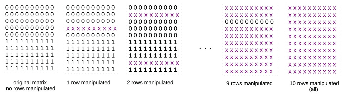
Figure 1: Schematic representation of the matrices of zeros and ones.
x x x x x x x x x x: row of ten real values randomly selected in the [0; 1] interval, for example: 0.22 0.93 0.67 0.34 0.51 0.49 0.28 0.12 0.46 0.10. At the beginning, the original matrix contains only zeros and ones: we apply -means with two clusters to it and save its results measured through the studied metrics. We then manipulate one randomly chosen row, by inserting real values randomly selected in the interval. Afterwards, we manipulate two, three, four randomly selected rows, and so on, until all the rows are completely manipulated. We apply -means with two clusters to each of these matrices and save its results measured through the studied metrics. If the values of a metric reflect this worsening, we can consider that metric stable. If not, we consider it unstable.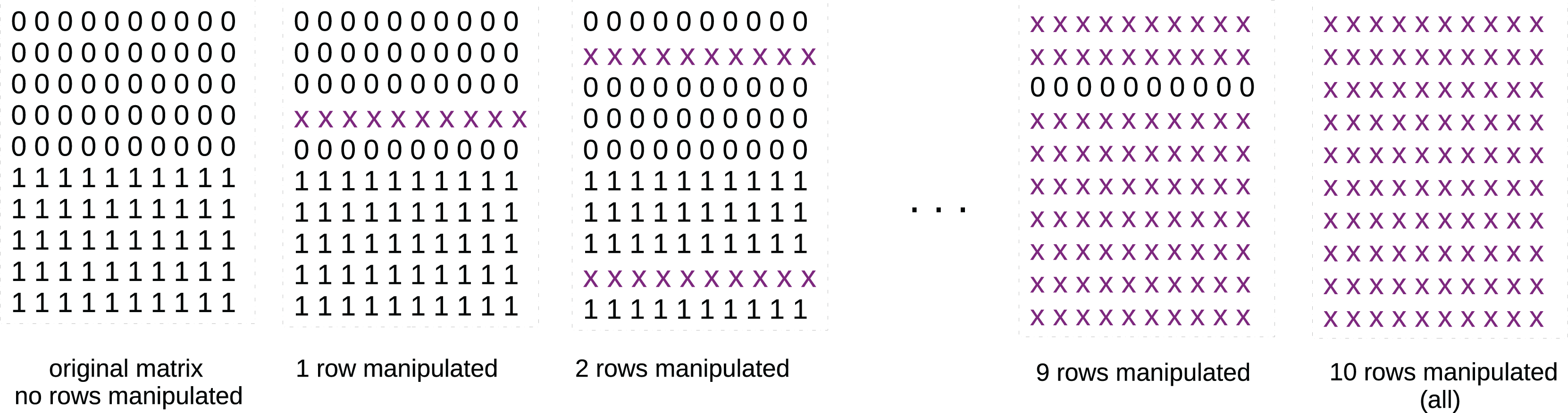
We then randomly selected a row and replaced it with real values in the interval, reapplied k-means, and calculated the analyzed metrics again. Afterwards, we randomly selected two, three, four rows and repeated the same procedures until we reached the total number of ten rows (Fig. 1). We saved the results of each metric at each step: since the matrix uniformity was clearly worsening at each iteration, we expected to see a worsening in the values of the metrics, too.
We analyzed the trends of the six analyzed metrics applied to the -means results obtained on the ten described matrices, and we noticed their trends (Fig. 2). The Silhouette coefficient, Davies-Bouldin index, Dunn index, and Calinski-Harabasz index showed a consistent (worsening) trend. Shannon entropy and Gap statistic, instead, showed an inconsistent trend.
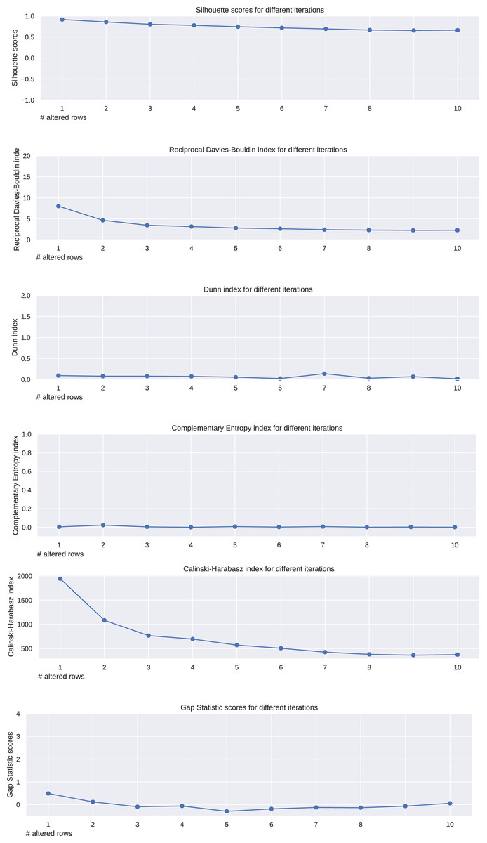
Figure 2: Results on the matrices of zeroes and ones for the Silhouette coefficient, Davies-Bouldin index, Dunn index, Shannon entropy, Calinski-Harabasz index, and Gap statistic.
Expected trend: worsening. Silhouette, reciprocal Davies-Bouldin, Dunn, Calinski-Harabasz observed trends: worsening. Complementary Shannon observed entropy trend: unchanged. Gap statistic observed trend: irregular.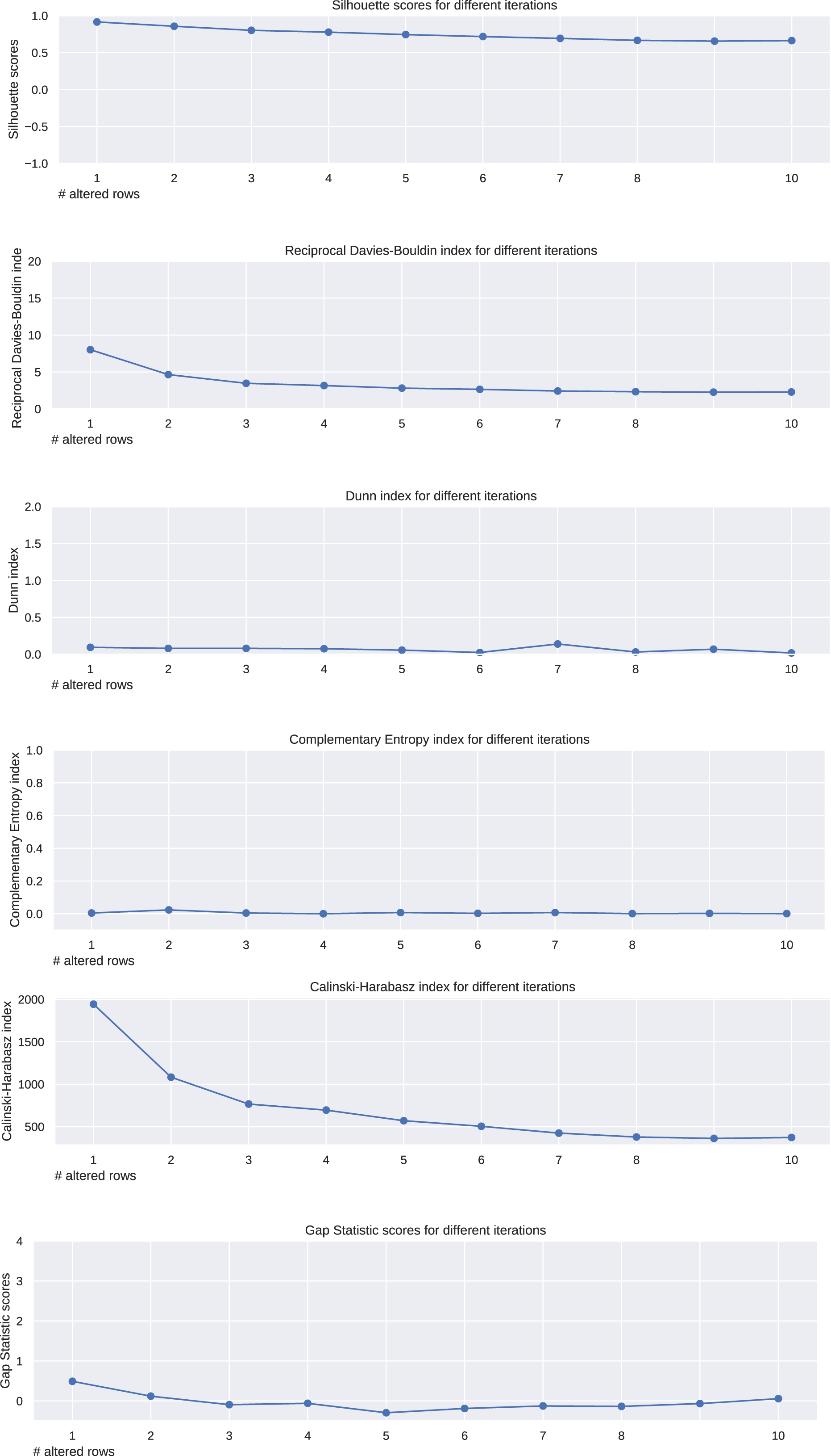
Artificial groups of points
We then utilized a series of artificial datasets inspired by the documentation of the scikit-learn Python package (scikit-learn, 2025a). We selected the cases where two distinct clusters of points were initially recognizable, and then we increasingly manipulated the initial data until no clear cluster was visible. We employed 5.000 points for each artificial dataset, except for the one where that number was insufficient to show relevant trends, and where we employed 10.000 points instead. At each step, we applied the -means clustering method by using clusters, and calculated all the six analyzed metrics on its results. This change of positions of the points clearly indicates a worsening of the separation of the two clusters, and therefore we studied the six metrics to understand if they would confirm or not this worsening. We applied the changes of points by using different standard deviations for the centers of the clusters of blobs of points (cluster_std parameter in the make_blob() function of the scikit-learn Python library (scikit-learn, 2025b)).
Since we focus our study on convex-shaped clusters, we avoided the nested, concave sets of points. We eventually observed the plotted trends of the values of the six metrics studied, and considered regular the trends that result constantly decreasing, constantly stable, or constantly increasing. We considered irregular all the trends that had locally divergent points (that are, local minima or local maxima).
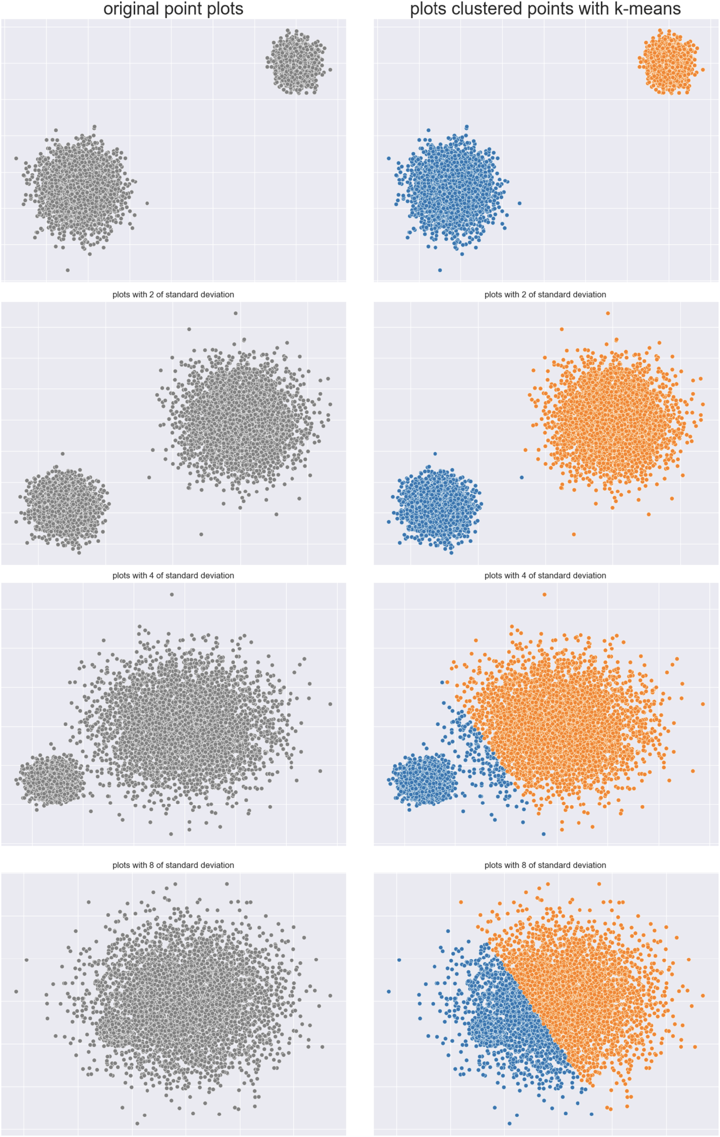
Clouds dataset: The first case included two clouds of points, initially clearly separated, that end up into a common cloud (Fig. 3).
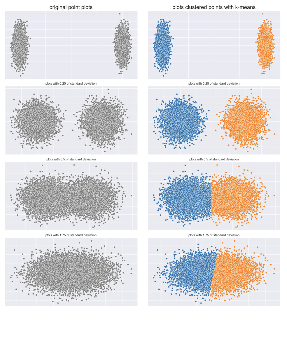
Figure 3: Clouds of points.
Two clouds original dataset (left) and results obtained by -means (right).
We applied -means and calculated the six metrics on ten cases (more than what shown in Fig. 3), and depicted their trends in Fig. 4.
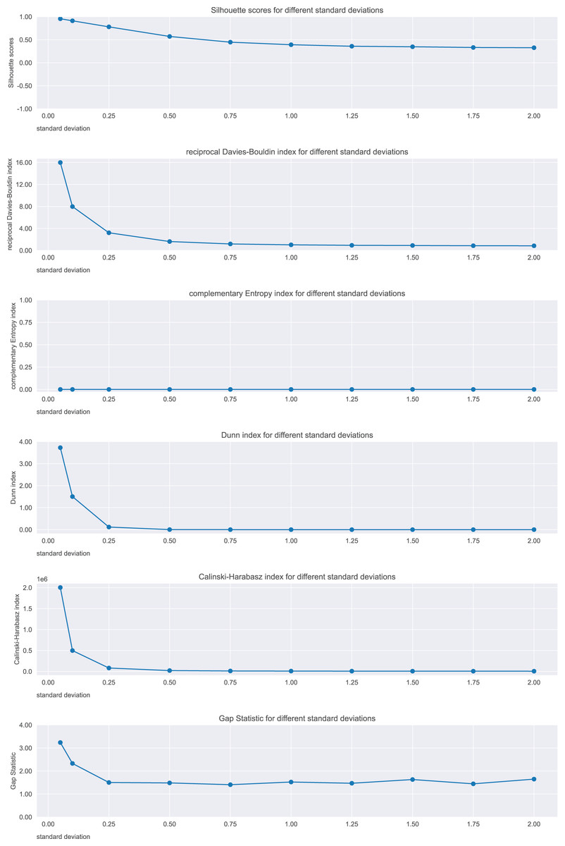
Figure 4: Results on the clouds dataset for the Silhouette coefficient, Davies-Bouldin index, Dunn index, Shannon entropy, Calinski-Harabasz index, and Gap statistic.
Standard deviation refers to the points generation. Expected trend: worsening. Silhouette, Reciprocal Davies-Bouldin, Dunn, Calinski-Harabasz observed trends: worsening. Complementary Shannon entropy observed trend: unchanged. Gap statistic observed trend: irregular.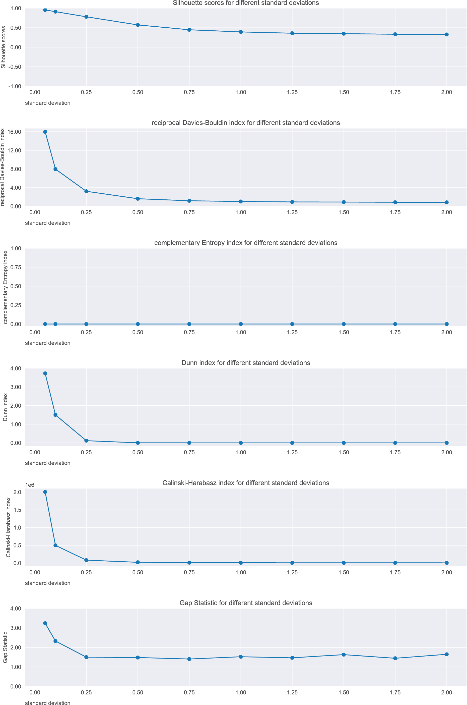
Silhouette, Davies-Bouldin index, Dunn index, Calinski-Harabasz index, and Gap statistic showed consistent trends, indicating the worsening of the clustering. In contrast, the Shannon entropy did not.
Semicircles dataset: We repeated the same controlled experiment described earlier on an artificial dataset made of two semicircles. These two semicircles are first merged together and then start to diverge, by creating two distinct clusters eventually (Fig. 5). We applied -means with clusters to these datasets, by changing standard deviations of the distributions of the point generation, and computed the six analyzed metrics. In the end, we checked which of these metrics would confirm the clustering trend, that is the improvement on distinguishing the two clusters.
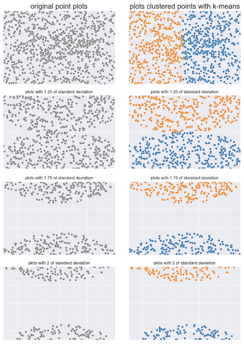
Figure 5: Semicircles of points.
Two semicircles original dataset (left) and results obtained by -means (right).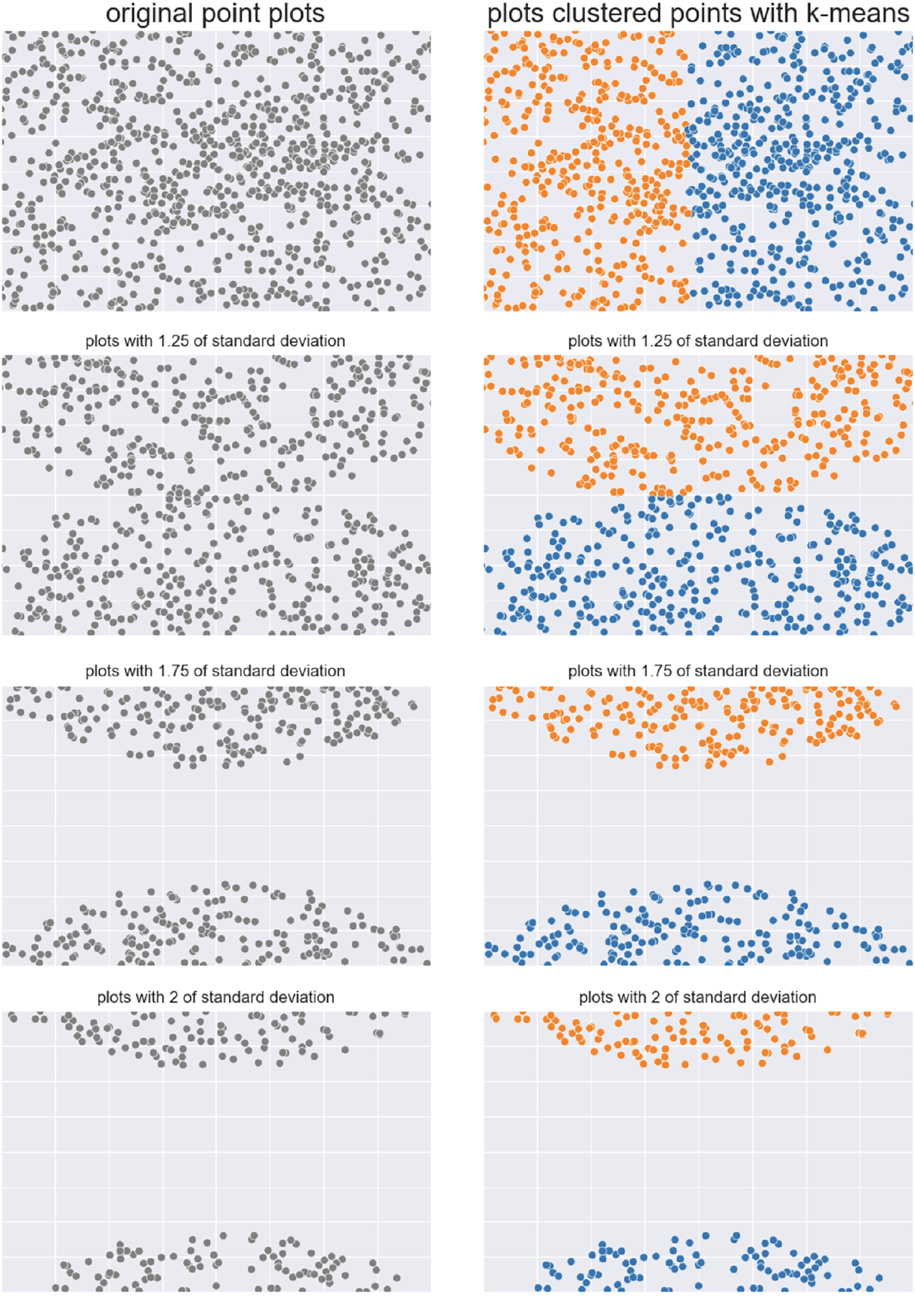
We depicted the trends of the six analyzed coefficients in six cases in Fig. 6.
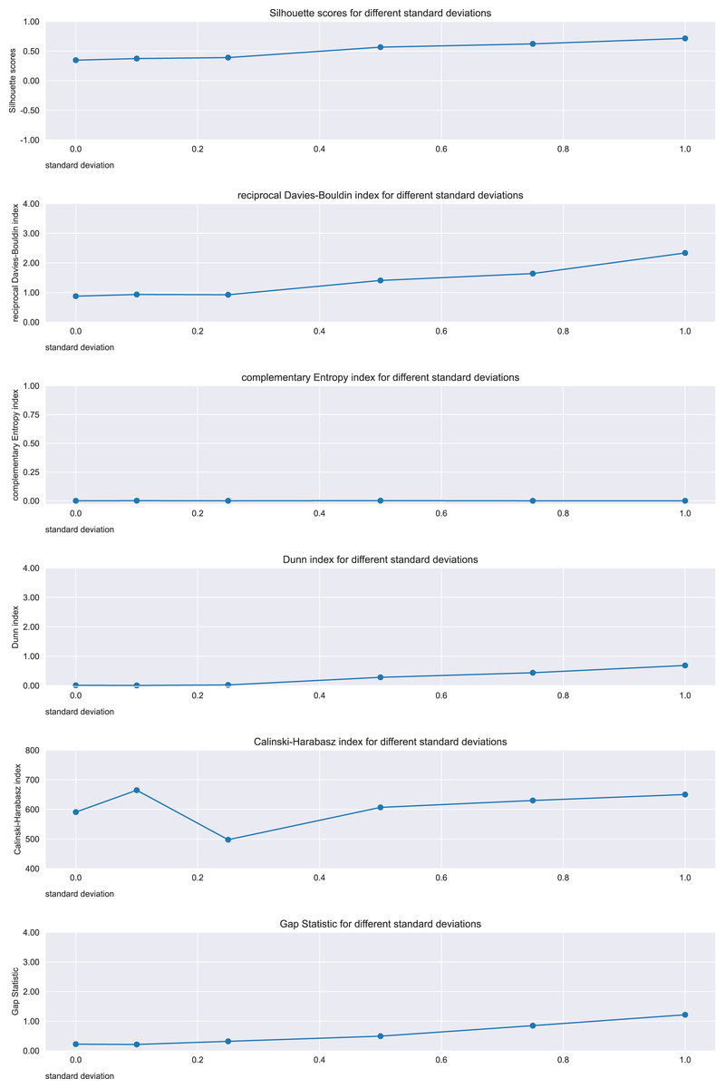
Figure 6: Results on the semicircles dataset for the Silhouette coefficient, Davies-Bouldin index, Dunn index, Shannon entropy, Calinski-Harabasz index, and Gap statistic.
Expected trend: increasing. Silhouette, reciprocal Davies-Bouldin, Dunn, Gap statistic observed trends: increasing. Complementary Shannon entropy observed trend: unchanged. Calinski-Harabasz observed trend: irregular.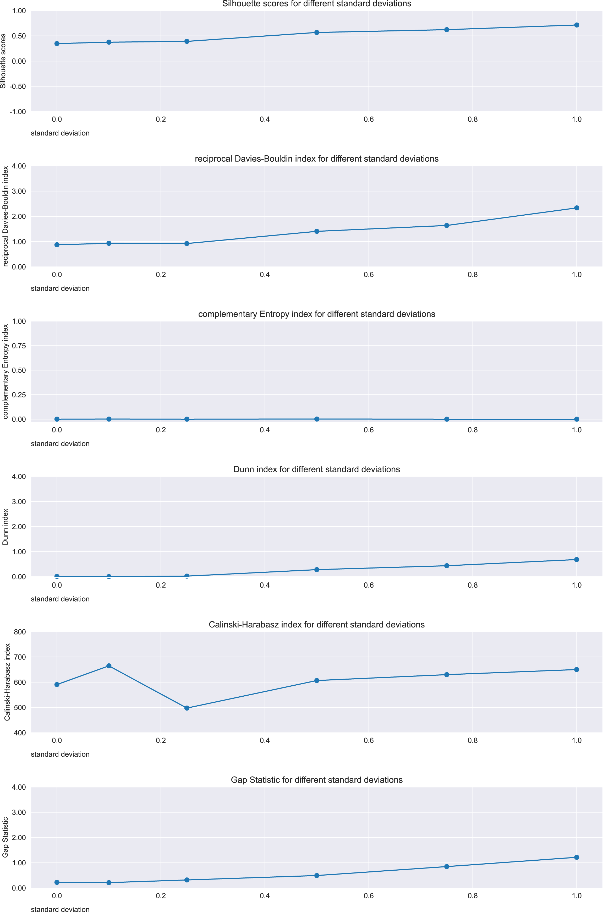
On these semicircles points, the metrics that consistently confirmed the improvement in the cluster separations were Silhouette, Davies-Bouldin index, Dunn index, and Gap statistic. On the other hand, Shannon entropy and Calinski-Harabasz index trends did not show any improvement.
Ball dataset: We repeated the same experiment on a dataset made of two balls, initially clearly separated, and eventually all mixed up. The ball on the right, in fact, increases its size until it joins the other ball, indicating a clear worsening regarding cluster separation (Fig. 7).
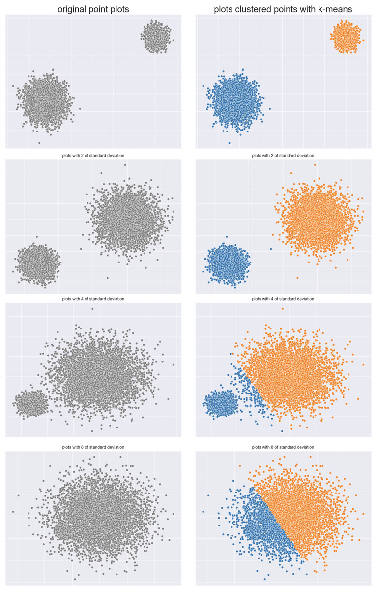
Figure 7: Two balls original dataset (left) and results obtained by -means (right).
We calculated the analyzed six metrics on seven distinct cases, and represented their trends in Fig. 8.
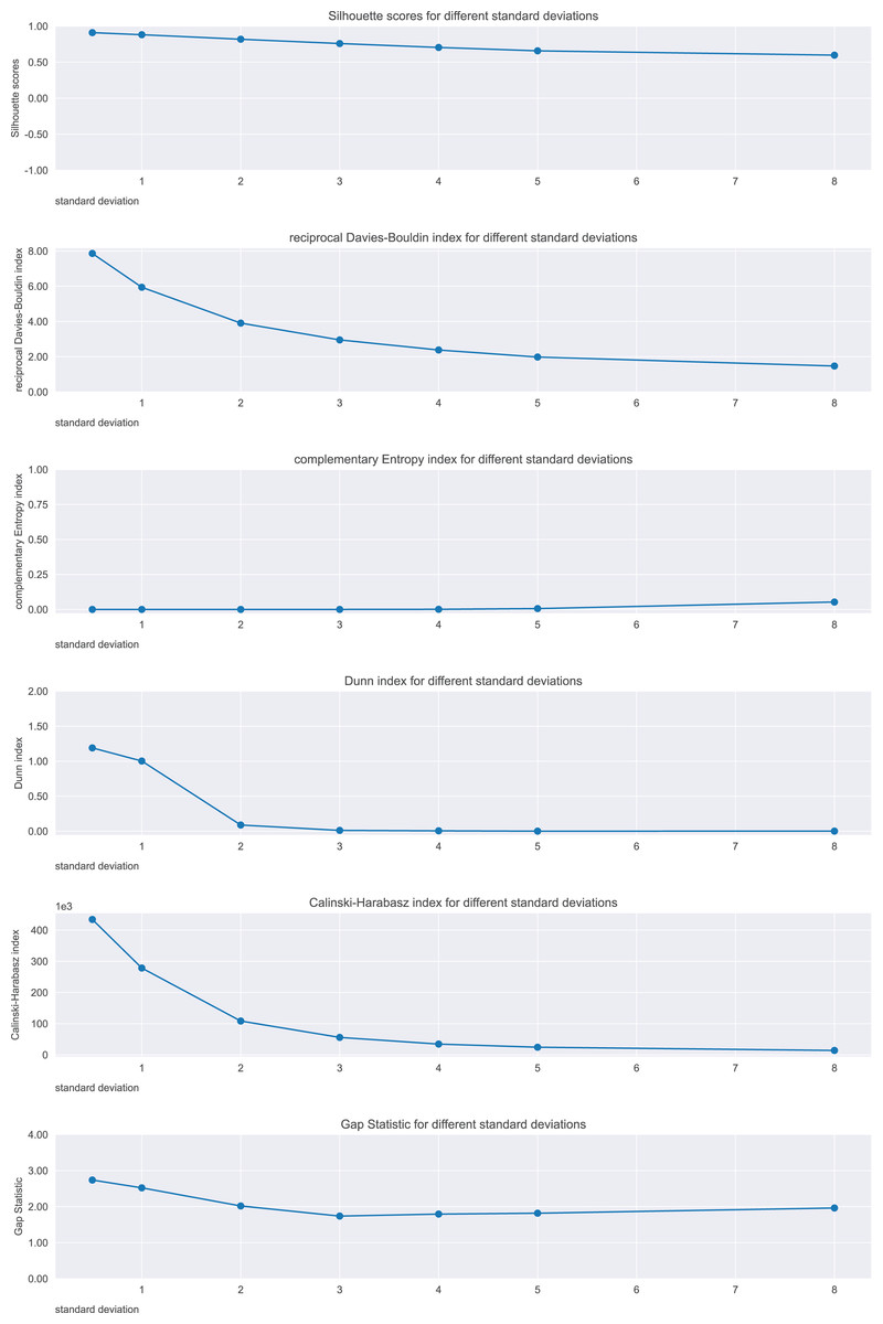
Figure 8: Results on the balls dataset for the Silhouette coefficient, Davies-Bouldin index, Dunn index, Shannon entropy, Calinski-Harabasz index, and Gap statistic.
Expected trend: worsening. Silhouette, reciprocal Davies-Bouldin, Dunn, Gap statistic observed trends, Calinski-Harabasz: worsening. Complementary Shannon entropy observed trend: unchanged.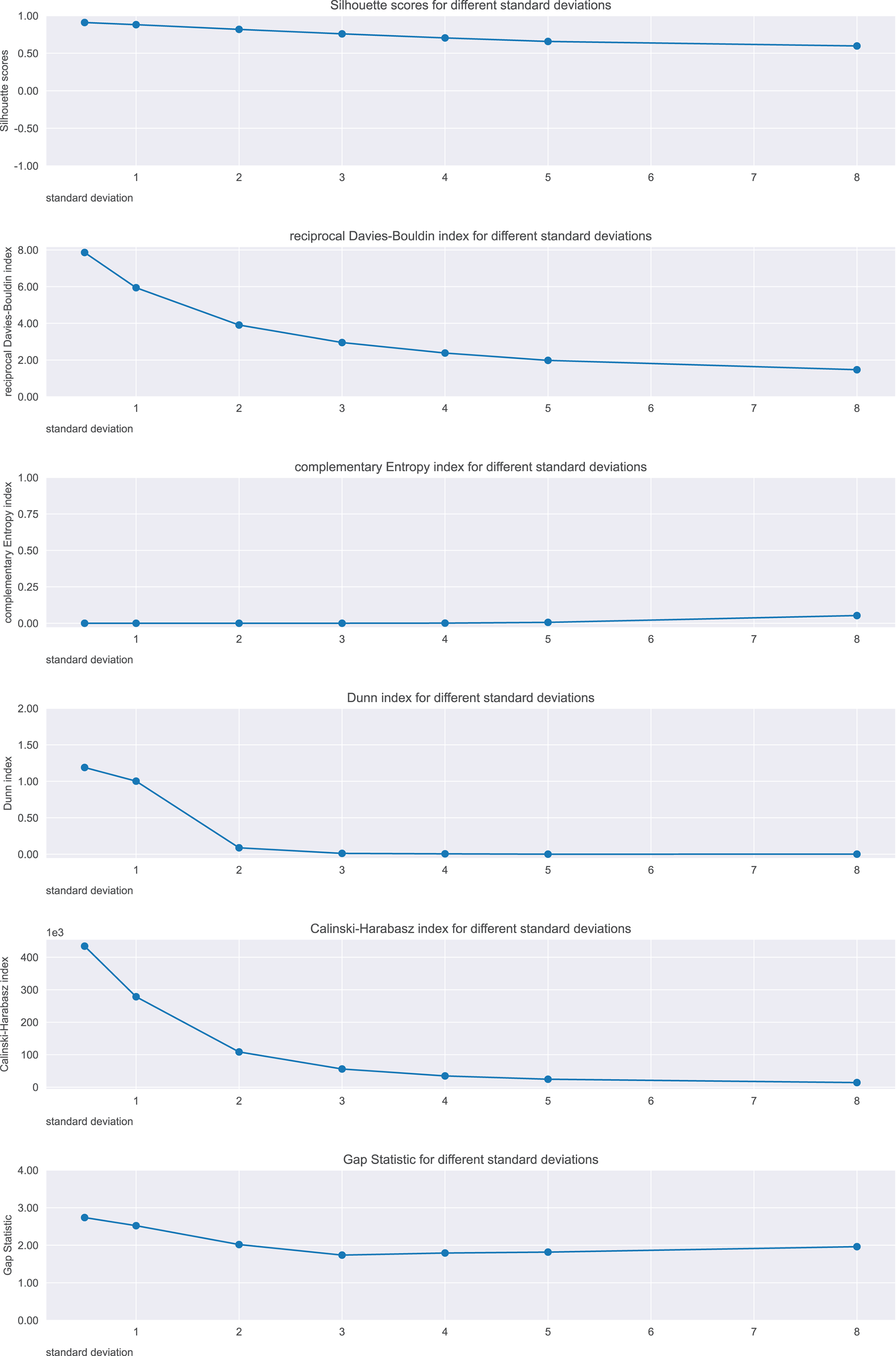
To summarize, the Silhouette coefficient, Calinski-Harabasz index, Davies-Bouldin index, and Dunn index confirmed the worsening trend of the ball clusters. Shannon entropy and Gap statistic, instead, did not.
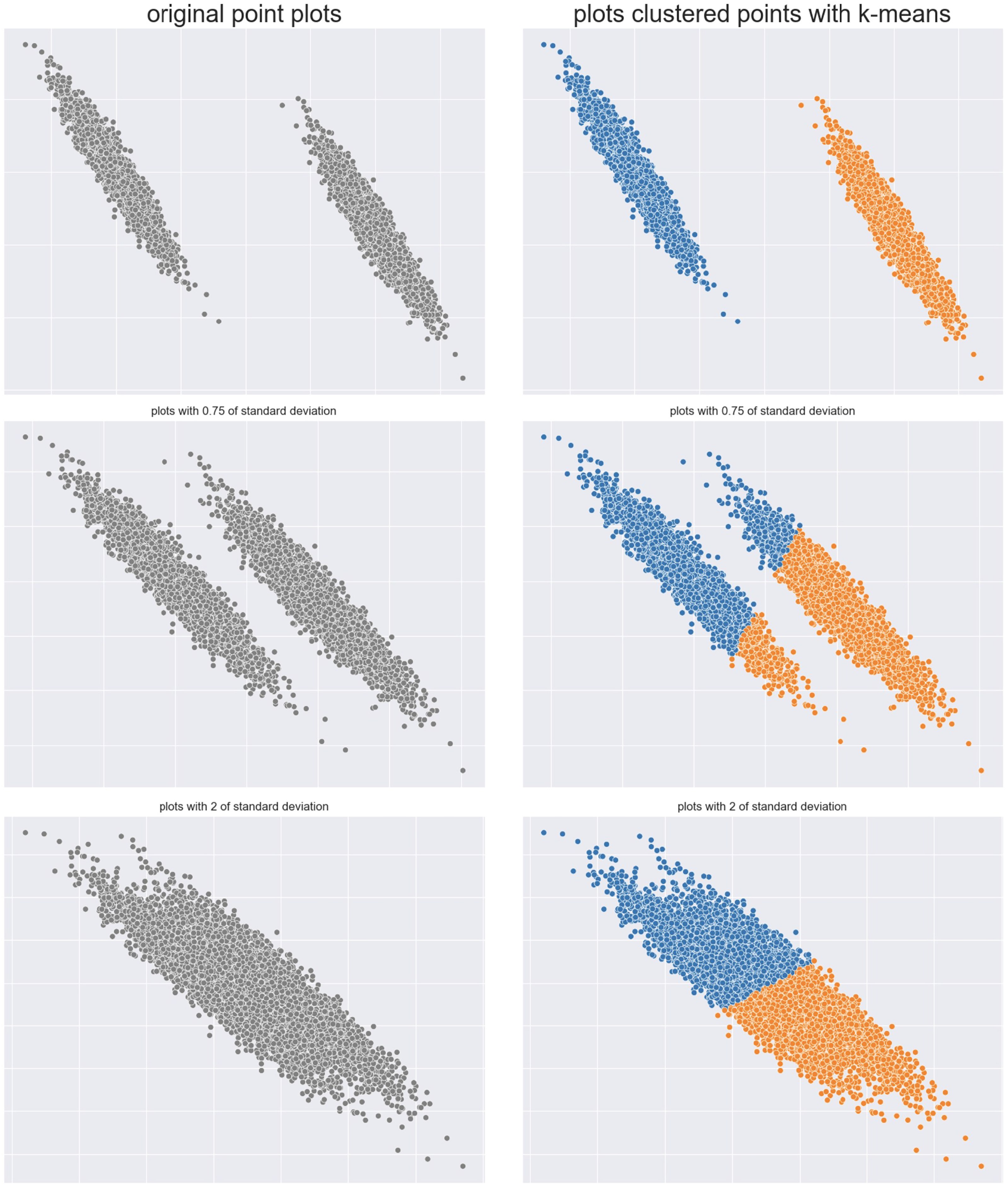
Brush strokes dataset: We then selected two sets of points that look like brush strokes: initially, they are clearly separated, but in the next plots they both move close to each other, until they end up into a single shape (Fig. 9), by changing the standard deviation. Again, we applied -means with and calculated the six analyzed internal clustering metrics at each step.
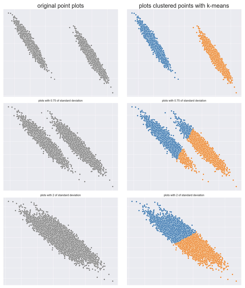
Figure 9: Two brush strokes original dataset (left) and results obtained by -means (right).
We depicted the trends of the six analyzed coefficient at seven different steps in Fig. 10.
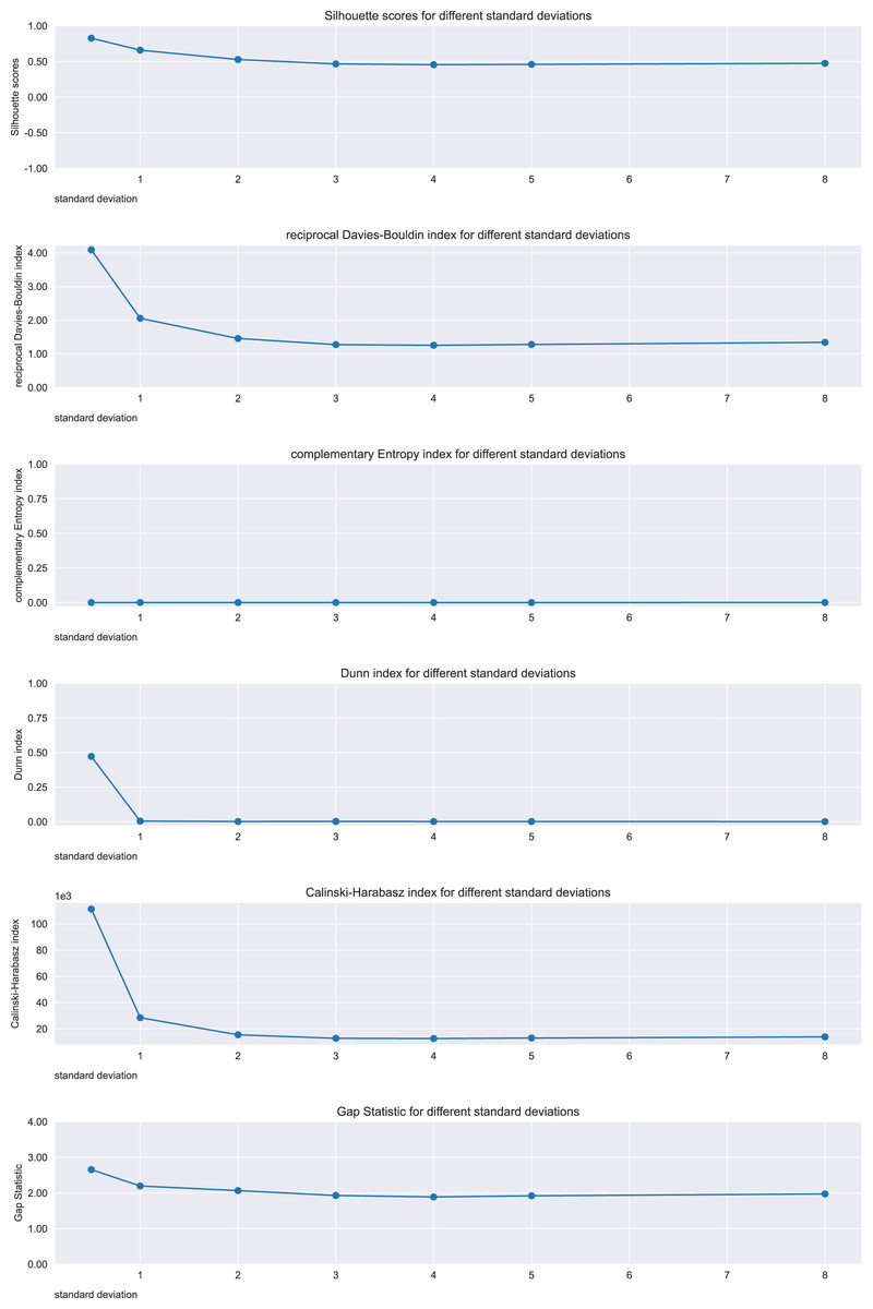
Figure 10: Results on the brush strokes dataset for the Silhouette coefficient, Davies-Bouldin index, Dunn index, Shannon entropy, Calinski-Harabasz index, and Gap statistic.
Expected trend: worsening. Silhouette, reciprocal Davies-Bouldin, Dunn, Gap statistic observed trends, Calinski-Harabasz: worsening. Complementary Shannon entropy observed trend: unchanged.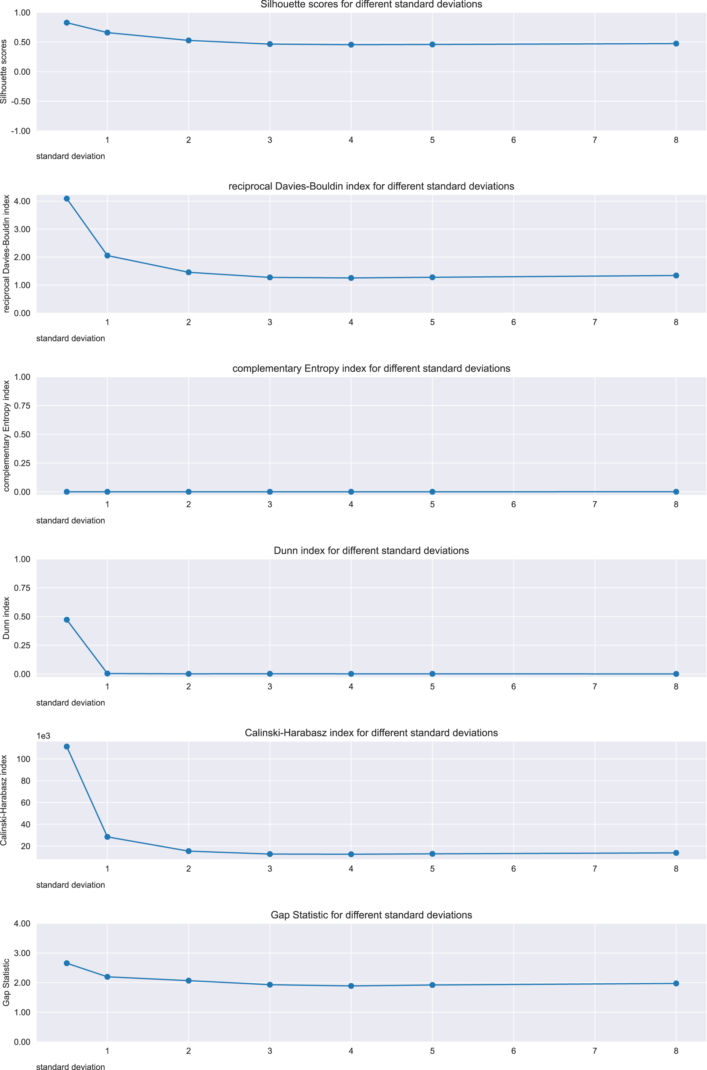
The trends of five considered metrics (Silhouette coefficient, Calinski-Harabasz index, Davies-Bouldin index, Gap statistic, and Dunn index) resulted being consistent with the worsening, while Shannon entropy’s trend resulted being inconsistent with the cluster separation worsening.
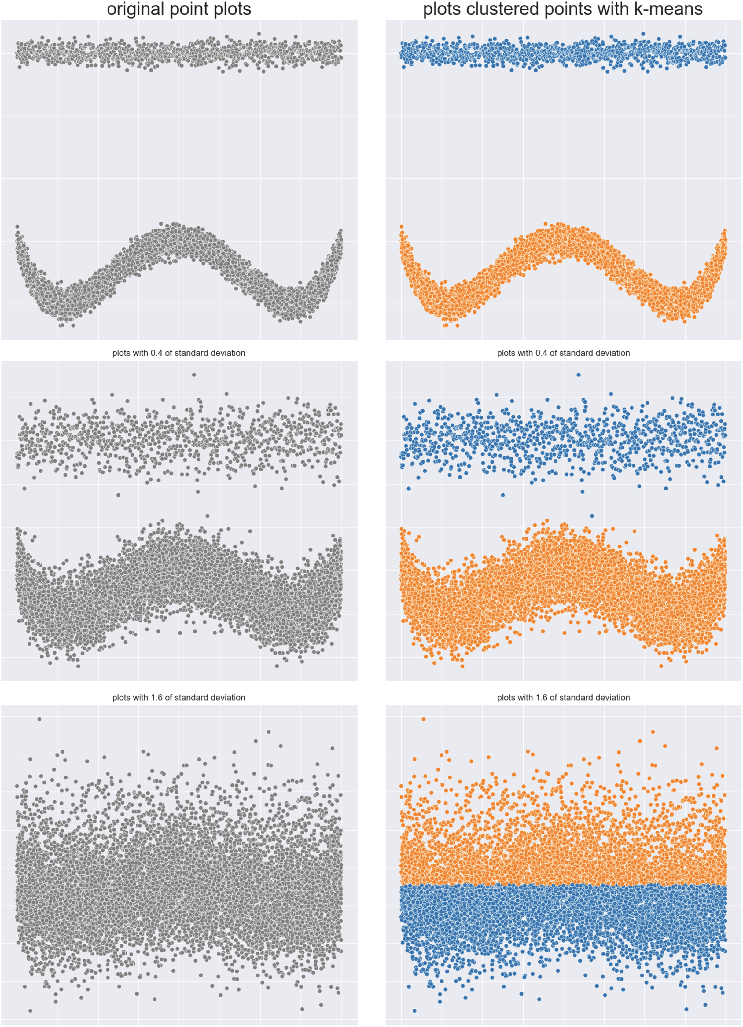
Dataset: The two clusters here initially are a straight horizontal line on the top and W-shaped set of points on the bottom. We randomly changed the distributions of these groups of points in the following steps, so that no shape would be recognizable in the end (Fig. 11). Again, we executed -means clustering by using , and calculated the six analyzed internal metrics.
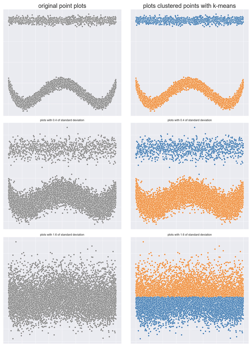
Figure 11: original dataset (left) and results obtained by -means (right).
Figure 12 represents the trends of the six analyzed measures at each step.
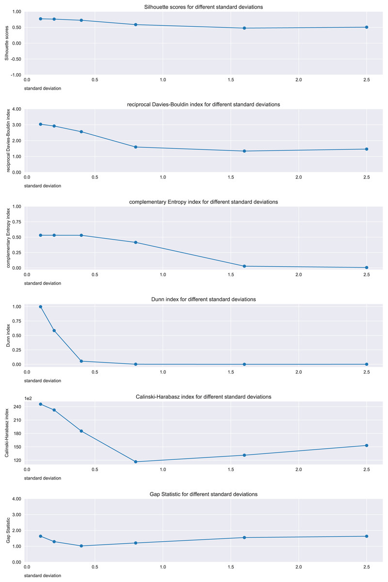
Figure 12: Results on the dataset for the Silhouette coefficient, Davies-Bouldin index, Dunn index, Shannon entropy, Calinski-Harabasz index, and Gap statistic.
Expected trend: worsening. Silhouette, reciprocal Davies-Bouldin, complementary Shannon entropy, Dunn index observed trends: worsening. Calinski Harabasz and Gap Statistic observed trends: irregular.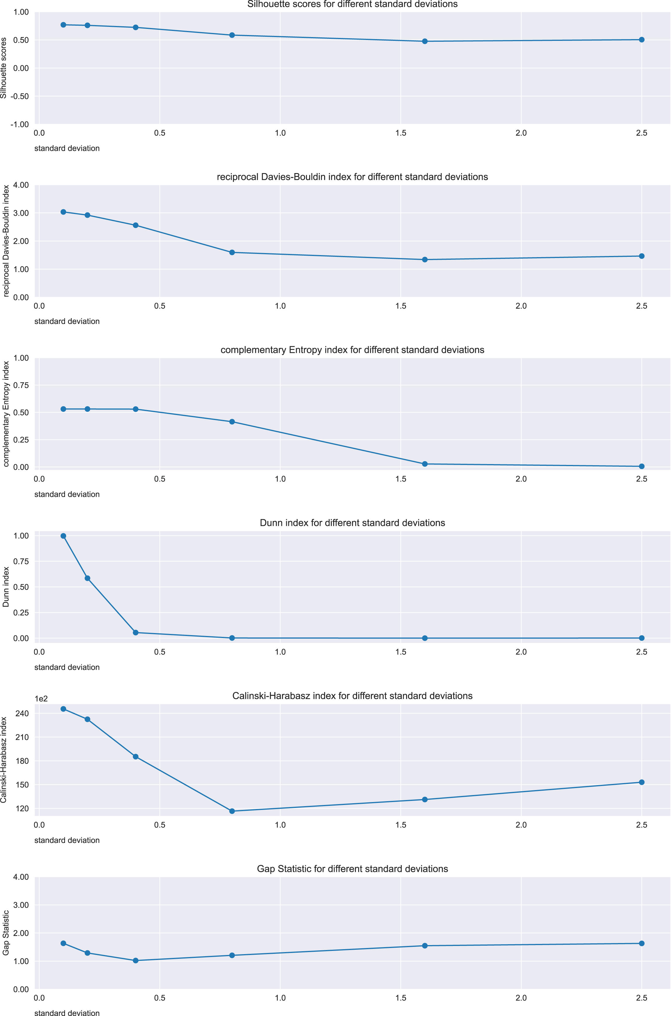
Regarding the worsening trend of this case, the Silhouette coefficient, Davies-Bouldin index, Shannon entropy, and Dunn index confirmed this outcome. The trends of Calinski-Harabasz index and Gap statistic, instead, did not show any worsening.
Artificial dataset test recap: After performing the just-described tests on the five artificial datasets, we summarized the results in Table 2.
| Ranking | Metric | Consistent | Trends |
|---|---|---|---|
| 1 | Silhouette coefficient | 5 out of 5 | 100% |
| 1 | Davies-Bouldin index | 5 out of 5 | 100% |
| 1 | Dunn index | 5 out of 5 | 100% |
| 4 | Calinski-Harabasz index | 3 out of 5 | 60% |
| 4 | Gap statistic | 3 out of 5 | 60% |
| 6 | Shannon entropy | 1 out of 5 | 20% |
As one can notice, the Silhouette coefficient, Davies-Bouldin index, and Dunn index produced consistent outcomes with the trends we expected to see in all the five scenarios (that means, worsening values while the cluster separation was worsening, and improving values while the cluster separation was improving). Calinski-Harabasz and Gap statistic resulted being consistent in three cases out of five, and Shannon entropy only once (Table 2). However, regarding results on bad clusters, when the clouds of points are indistinguishable (right end of the previous plots (Figs. 4, 6, 8, 10, and 12), we can see that Davies-Bouldin index always stays around 0 (as expected), while the Silhouette coefficient lays around +0.5. In these cases, we can state that Silhouette shows an inconsistent outcome with respect to the clustering results: in the right end of these plots, we would expect Silhouette to get a value around 0 or , which never happens. This behavior is a flaw of the Silhouette coefficient that needs to be considered.
To recap, these results indicate a higher reliability and effectiveness of the Silhouette coefficient, Davies-Bouldin index, and Dunn index compared with the other analyzed metrics for internal clustering evaluation, with the Silhouette score having the just-mentioned flaw for bad clustering results.
Real-world medical scenarios
To test the effectiveness and the reliability of the six metrics considered in this study, we developed an approach based on clustering applied to data of real-world electronic health records (EHRs) of patients with different diseases (Boonstra, Versluis & Vos, 2014).
Electronic health records (EHRs) are digital information reports designed to collect, store, and provide healthcare data in computer-readable format (Kim et al., 2019). The information contained in EHRs generally includes essential demographic details like date of birth and sex at birth, along with data on diagnoses, treatments, clinical investigation results, and outcomes such as hospital discharge or death. EHRs collect data at the individual level, and by using unique patient identifiers, it becomes possible to track various aspects of care and outcomes over time (Cowie et al., 2017). The real-world data derived from EHRs can be valuable for researchers focused on understanding health and disease, identifying disease trajectories, and assessing disease risks and treatments through modern statistical and machine learning methods (Aminoleslami, Anderson & Chicco, 2024).
These data were collected for clinical reasons, and not for scientific reasons, and therefore have a high level of complexity, especially for clustering purposes it is even possible that no meaningful partition of patients among these data exists. For these reasons, we decided to employ these datasets for our study: if any cluster is found, we can be confident that no “shortcut” or pre-arranged setting generated them. If a cluster is found, it is because of the clustering algorithm used.
Euclidean similarity clustering. Among the measures for external clustering validity, there is consensus about the usage of the ARI (Hubert & Arabie, 1985), that necessitates of an external ground truth. Since we are studying convex-shaped clusters and are focusing this study on -means with Euclidean distance, we developed a new clustering approach based on the Euclidean similarity between couples of rows. We set k = 2 clusters and apply this approach to each single dataset: we assign the first row to the cluster A, and then we assign all the other rows of the dataset having Euclidean similarity to the initial row to the same cluster A. We measure the similarity by computing the Euclidean distance between two rows, and using a particular threshold. If we find a row that is not enough similar to the first row (and therefore its similarity is above the threshold), we assign it to the cluster B. Then we cycle on the remaining rows to see if any of them is similar to the row assigned to cluster B, and, if found, we put it in cluster B. We called this approach Euclidean similarity clustering (ESC) and we describe it more in detail in Algorithm 1 and in Fig. 13.
| 1: Read the dataset with N rows and M columns |
| 2: rA ← r1, assign rA to cluster A |
| 3: for each other row rx with : |
| 4: if(Euclidean distance (rA, rx) > t): rB ← rx, assign rB to cluster B, and stop for |
| 5: for each other row ry with : |
| 6: if(Euclidean distance (rA, ry) ≤ t): assign ry to cluster A |
| 7: elseif(Euclidean distance (rB, ry) ≤ t): assign ry to cluster B |
| 8: else discard the ry point |
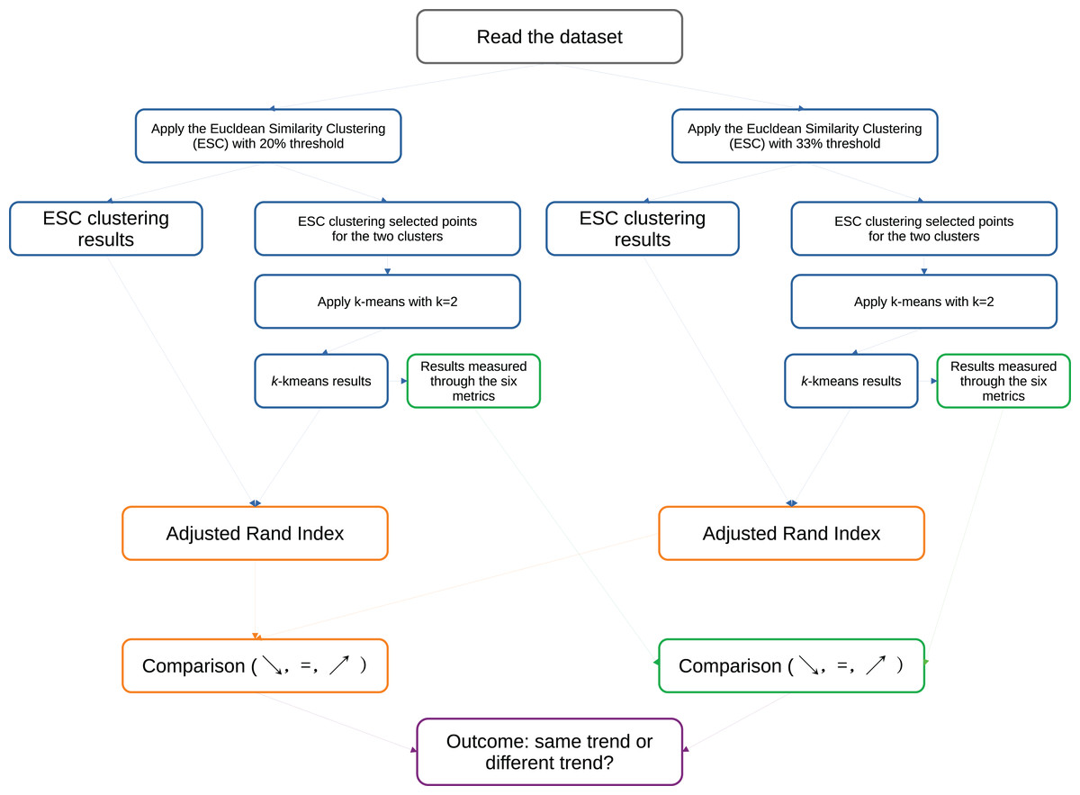
Figure 13: Schematic representation of our algorithm to assess the reliability of the six analyzed metrics on the medical datasets.
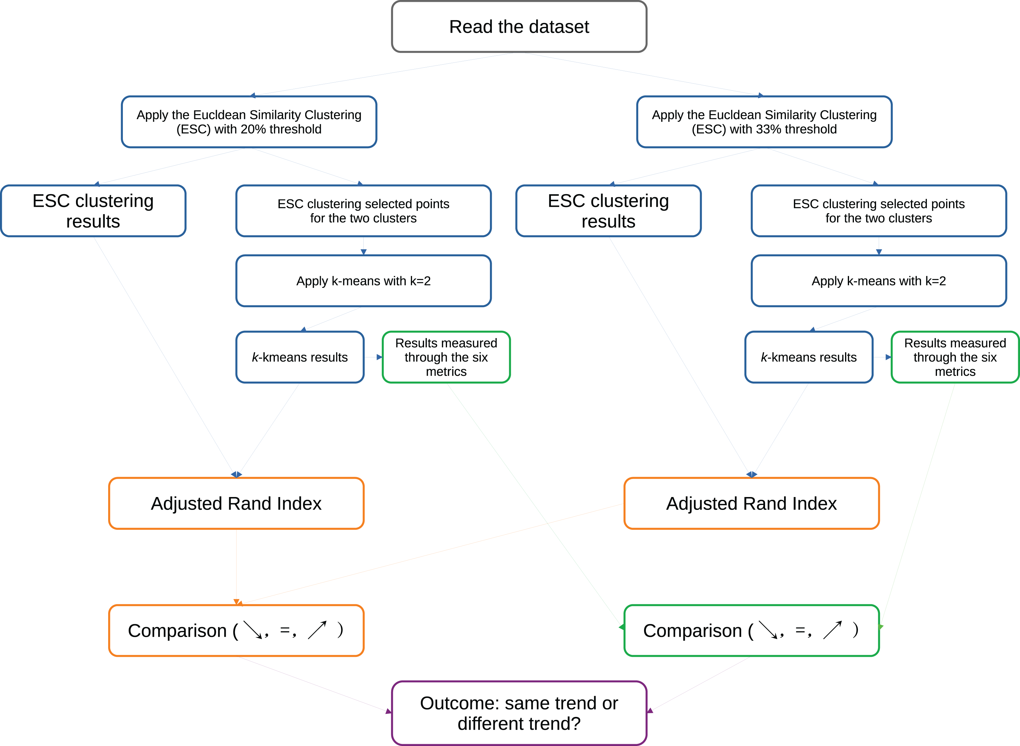
The rationale behind this algorithm is as follows. If the Euclidean distance between two data rows is lower than a specific relative threshold, we consider both data rows to be part of the same cluster. Conversely, if the Euclidean distance between two data rows is high, we do not consider them to belong to the same cluster. Since we based our entire study on two clusters, we also utilize only two clusters for the ESC. Given that we employ -means clustering based on Euclidean distance, we regard the clusters identified by this ESC method as a form of “ground truth” for assessing the results of our clustering coefficients.
After applying the ESC algorithm, we execute -means with on all the rows found by ESC in its two clusters, and we measure its results through the six metrics for the internal clustering validation. We use the results of ESC as gold standard for the results of -means, and we compute the adjusted Rand index between them (Algorithm 2 and Fig. 13).
| 1: Read a single EHRs dataset |
| 2: Apply the Euclidean similarity clustering (ESC) algorithm (Algorithm 1) and save the content of its two output clusters |
| 3: Apply k-means with on the data within the two clusters of ESC computed at the previous step, and save the content of its two output clusters |
| 4: Calculate the six studied metrics on the results of k-means obtained at the previous step |
| 5: Calculate the adjusted Rand index (ARI) between the ESC clustering results (line 2) and the results of k-means (line 3) |
Coefficients’ trends at varying thresholds: We performed two tests for each dataset: one by using the 20% similarity threshold, and then another one by employing the 33% threshold instead: the former is stricter and selects only data rows similar between each other, and the latter is a bit more permissive. Afterwards, we checked the values of the adjusted Rand index and the values of the six metrics for the scenarios of both similarity thresholds. We observed six possible scenarios for each metric (Silhouette coefficient, Davies-Bouldin index, Calinski-Harabasz index, Dunn index, Shannon entropy and Gap statistic) when moving from the 20% case to the 33% case:
If the values of the adjusted Rand indices were similar (=), and the values of the analyzed metric were similar (=), we considered this trend consistent;
If the values of the adjusted Rand indices were similar (=), but the values of the analyzed metric were increasing ( ) or decreasing ( ), we considered this trend inconsistent;
If the values of the adjusted Rand indices were decreasing ( ), and the values of the analyzed metric were decreasing ( ), we considered this trend consistent;
If the values of the adjusted Rand indices were increasing ( ), and the values of the analyzed metric were increasing ( ), we considered this trend consistent;
If the values of the adjusted Rand indices were increasing ( ), but the values of the analyzed metric were similar (=) or decreasing ( ), we considered this trend inconsistent;
If the values of the adjusted Rand indices were decreasing ( ), but the values of the analyzed metric were similar (=) or increasing ( ), we considered this trend inconsistent.
We consider two values of the same clustering metric similar if their absolute difference is lower than 20%. In the next tables, we call this difference quantitative consistency. That means, if the quantitative consistency of a specific metric value is lower than or lower than , we assign the stable sign tho that trend (=).
We described our approach more in detail in Fig. 13.
We explain how our algorithm works on a toy synthetic EHRs dataset that we represented fully in Table 3. In this toy dataset, each row represents the profile of single patient, and each column contains a clinical or demographic feature. The features indicate the age of the patients in years, the sex, the level of education and the stage of cancer, plus a column indicating the ID of the patient. As one can notice immediately, these invented data points can be easily clustered in two partitions by our ESC method: the first five rows belong to the cluster A, and the last five rows belong to cluster B.
| ID | Age | Sex | Education | Cancer stage |
|---|---|---|---|---|
| 1 | 5 | 0 | 1 | 1 |
| 2 | 6 | 0 | 1 | 1 |
| 3 | 5 | 0 | 1 | 1 |
| 4 | 4 | 0 | 1 | 1 |
| 5 | 6 | 0 | 1 | 1 |
| 6 | 80 | 1 | 4 | 4 |
| 7 | 79 | 1 | 4 | 4 |
| 8 | 78 | 1 | 4 | 4 |
| 9 | 78 | 1 | 4 | 4 |
| 10 | 81 | 1 | 4 | 4 |
After using the Euclidean similarity clustering method, we applied -means to its clusters, and compared the results of both algorithms by using the ARI. By using both the 20% and the 33% similarity thresholds, we notice that adjusted Rand indices are always +1 in the interval, which indicates perfect match (Table 4).
| Cluster | Cluster elements | % |
|---|---|---|
| Euclidean similarity clustering results with 20% threshold | ||
| 1st cluster | 5 patients out of 10 | 50.0 |
| 2nd cluster | 5 patients out of 10 | 50.0 |
| No cluster | 0 patients out of 10 | 0.0 |
| -means clustering results with 20% threshold | ||
| 1st cluster | 5 patients out of 10 | 50.0 |
| 2nd cluster | 5 patients out of 10 | 50.0 |
| No cluster | 0 patients out of 10 | 0.0 |
| ARI ( -means results, ESC results) = +1.00 | ||
| Euclidean similarity clustering results with 33% threshold | ||
| 1st cluster | 5 patients out of 10 | 50 |
| 2nd cluster | 5 patients out of 10 | 50 |
| No cluster | 0 patients out of 10 | 0 |
| -means clustering results with 33% threshold | ||
| 1st cluster | 5 patients out of 10 | 50 |
| 2nd cluster | 5 patients out of 10 | 50 |
| No cluster | 0 patients out of 10 | 0 |
| ARI ( -means results, ESC results) = +1.00 | ||
| ARI trend: stable (=) 0% | ||
The clustering internal metrics computed on the results of -means applied to the elements grouped in the two clusters by the Euclidean similarity clustering (ESC) (Table 5) are identical for the 20% and 33% threshold cases (=) and confirm the trend of the ARI computed earlier (Table 4): in this case, we can consider the trends of all the six metrics consistent with the trends of ARI. All the six metrics passed this sanity check.
| 20% threshold | 33% threshold | Quantitative consistency |
Trend | Trend consistency with ARI trend |
|
|---|---|---|---|---|---|
| Silhouette coefficient | 0.991 | 0.991 | 0% | = | Consistent |
| Complementary Shannon entropy | 0.000 | 0.000 | 0% | = | Consistent |
| Calinski-Harabasz index | 48,464.583 | 48,464.583 | 0% | = | Consistent |
| Reciprocal Davies-Bouldin index | 90.787 | 90.787 | 0% | = | Consistent |
| Dunn index | 75.781 | 75.781 | 0% | = | Consistent |
| Gap statistic | 7.278 | 7.278 | 0% | = | Consistent |
Sepsis and SIRS EHRs dataset: We executed our just-described algorithm on a dataset of real-world electronic medical records of Turkish patients who had sepsis or systemic inflammatory response syndrome (SIRS) (Gucyetmez & Atalan, 2016). S This dataset table contains 1,257 patient profiles (rows) and 16 clinical variables (columns), without missing data. We applied our proposed our ESC approach and -means first with a 20% similarity threshold and then with a 33% threshold, and we noticed that the ARI value moved from 1 to 0.318 (Table 6).
| Cluster | Cluster elements | % |
|---|---|---|
| Euclidean similarity clustering results with 20% threshold | ||
| 1st cluster | 226 patients out of 1,257 | 17.979 |
| 2nd cluster | 187 patients out of of 1,257 | 14.877 |
| No cluster | 844 patients out of 1,257 | 67.144 |
| -means clustering results with 20% threshold | ||
| 1st cluster | 226 patients out of 1,257 | 17.979 |
| 2nd cluster | 187 patients out of 1,257 | 14.877 |
| No cluster | 844 patients out of 1,257 | 67.144 |
| ARI ( -means results, ESC results) = +1.000 | ||
| Euclidean similarity clustering results with 33% threshold | ||
| 1st cluster | 883 patients out of 1,257 | 70.246 |
| 2nd cluster | 169 patients out of 1,257 | 13.444 |
| No cluster | 205 patients out of 1,257 | 16.309 |
| -means clustering results with 33% threshold | ||
| 1st cluster | 388 patients out of 1,257 | 30.867 |
| 2nd cluster | 664 patients out of 1,257 | 52.824 |
| No cluster | 205 patients out of 1,257 | 16.309 |
| ARI ( -means results, ESC results) = +0.318 | ||
| ARI trend: decrease ( ) | ||
We then calculated the six analyzed metrics on the results of -means and checked their trends when changing similarity thresholds (Table 7). The Silhouette coefficient, Davies-Bouldin index, Dunn index, and Gap statistic confirmed the decreasing trend, while Shannon entropy and Calinski-Harabasz index resulted being inconsistent with the ARI trend.
| 20% threshold | 33% threshold | Quantitative consistency |
Trend | Trend consistency with ARI trend |
|
|---|---|---|---|---|---|
| Silhouette coefficient | 0.491 | 0.364 | –26% | Consistent | |
| Complementary Shannon entropy | 0.006 | 0.050 | +733% | Inconsistent | |
| Calinski-Harabasz index | 499.571 | 560.611 | +12% | = | Inconsistent |
| Reciprocal Davies-Bouldin index | 1.155 | 0.816 | –29% | Consistent | |
| Dunn index | 0.729 | 0.044 | –94% | Consistent | |
| Gap statistic | 0.987 | 0.731 | –26% | Consistent |
Depression and heart failure EHRs dataset
We executed again algorithm on a dataset of real-world electronic medical records of patients diagnosed with depression and heart failure (Jani et al., 2016), collected in Minnesota, USA.
This dataset table contains 425 patient profiles (rows) and 15 clinical factors (columns), without missing data. We applied our proposed our ESC approach and -means first with a 20% similarity threshold and then with a 33% threshold, and we noticed that the ARI value decreased from 1 to 0.179 (Table 8).
| Cluster | Cluster elements | % |
|---|---|---|
| Euclidean similarity clustering results with 20% threshold | ||
| 1st cluster | 7 patients out of 425 | 1.647 |
| 2nd cluster | 4 patients out of 425 | 0.941 |
| No cluster | 414 patients out of 425 | 97.412 |
| -means clustering results with 20% threshold | ||
| 1st cluster | 4 patients out of 425 | 0.941 |
| 2nd cluster | 7 patients out of 425 | 1.647 |
| No cluster | 414 patients out of 425 | 97.412 |
| ARI ( -means results, ESC results) = +1.000 | ||
| Euclidean similarity clustering result with 33% threshold | ||
| 1st cluster | 55 patients out of 425 | 12.941 |
| 2nd cluster | 27 patients out of 425 | 6.353 |
| No cluster | 343 patients out of 425 | 80.706 |
| -means clustering results with 33% threshold | ||
| 1st cluster | 50 patients out of 425 | 11.765 |
| 2nd cluster | 32 patients out of 425 | 7.529 |
| No cluster | 343 patients out of 425 | 80.706 |
| ARI ( -means results, ESC results) = +0.179 | ||
| ARI trend: decrease ( ) | ||
We then calculated the six analyzed metrics on the results of -means and checked their trends when changing similarity thresholds (Table 9). The Silhouette coefficient, Davies-Bouldin index, Shannon entropy, and Gap statistic confirmed the decreasing trend, while Calinski-Harabasz index and Dunn index resulted being inconsistent with the ARI trend.
| 20% threshold | 33% threshold | Quantitative consistency |
Trend | Trend consistency with ARI trend |
|
|---|---|---|---|---|---|
| Silhouette coefficient | 0.616 | 0.263 | Consistent | ||
| Complementary Shannon entropy | 0.0543 | 0.0350 | Consistent | ||
| Calinski-Harabasz index | 28.434 | 30.785 | = | Inconsistent | |
| Reciprocal Davies-Bouldin index | 1.920 | 0.651 | Consistent | ||
| Dunn index | 1.460 | 0.193 | = | Inconsistent | |
| Gap statistic | 0.278 | 0.003 | Consistent |
Cardiac arrest EHRs dataset: We executed again algorithm on a dataset of real-world electronic medical records of patients who had an out-of-hospital cardiac arrest (Requena-Morales et al., 2017), collected in Spain.
This dataset table contains 422 patient profiles (rows) and 10 clinical factors (columns), without missing data. We applied our proposed our ESC approach and -means first with a 20% similarity threshold and then with a 33% threshold, and we noticed that the ARI value decreased from 1 to 0.47 (Table 10).
| Cluster | Cluster elements | % |
|---|---|---|
| Euclidean similarity clustering results with 20% threshold | ||
| 1st cluster | 27 patients out of 422 | 6.398 |
| 2nd cluster | 12 patients out of 422 | 2.844 |
| No cluster | 383 patients out of 422 | 90.758 |
| -means clustering results with 20% threshold | ||
| 1st cluster | 27 patients out of 422 | 6.398 |
| 2nd cluster | 12 patients out of 422 | 2.844 |
| No cluster | 383 patients out of 422 | 90.758 |
| ARI ( -means results,ESC results) = +1.000 | ||
| Euclidean similarity clustering results with 33% threshold | ||
| 1st cluster | 60 patients out of 422 | 14.218 |
| 2nd cluster | 43 patients out of 422 | 10.190 |
| No cluster | 319 patients out of 422 | 75.592 |
| -means clustering results with 33% threshold | ||
| 1st cluster | 60 patients out of 422 | 14.218 |
| 2nd cluster | 43 patients out of 422 | 10.190 |
| No cluster | 319 patients out of 422 | 75.592 |
| ARI ( -means results,ESC results) = +0.470 | ||
| ARI trend: decrease ( ) | ||
We then calculated the six analyzed metrics on the results of -means and checked their trends when changing similarity thresholds (Table 11). All the six metrics confirmed the decreasing trend of ARI.
| 20% threshold | 33% threshold | Quantitative consistency |
Trend | Trend consistency with ARI trend |
|
|---|---|---|---|---|---|
| Silhouette coefficient | 0.765 | 0.362 | Consistent | ||
| Complementary Shannon entropy | 0.110 | 0.020 | Consistent | ||
| Calinski-Harabasz index | 229.912 | 52.903 | Consistent | ||
| Reciprocal Davies-Bouldin index | 3.131 | 0.762 | Consistent | ||
| Dunn index | 1.776 | 0.035 | Consistent | ||
| Gap statistic | 0.878 | 0.099 | Consistent |
Neuroblastoma EHRs dataset: We executed again algorithm on a dataset of real-world electronic medical records of children suffering from neuroblastoma (Ma et al., 2018), collected in eastern China.
This dataset table contains 169 patient profiles (rows) and 13 clinical factors (columns), without missing data. We applied our proposed our ESC approach and -means first with a 20% similarity threshold and then with a 33% threshold, and we noticed that the ARI value decreased from 1 to 0.182 (Table 12).
| Cluster | Cluster elements | % |
|---|---|---|
| Euclidean similarity clustering results with 20% threshold | ||
| 1st cluster | 4 patients out of 169 | 2.367 |
| 2nd cluster | 8 patients out of 169 | 4.734 |
| No cluster | 157 patients out of 169 | 92.899 |
| -means clustering results with 20% threshold | ||
| 1st cluster | 8 patients out of 169 | 4.734 |
| 2nd cluster | 4 patients out of 169 | 2.367 |
| No cluster | 157 patients out of 169 | 92.899 |
| ARI ( -means results,ESC results) = +1.000 | ||
| Euclidean similarity clustering results with 33% threshold | ||
| 1st cluster | 25 patients out of 169 | 14.793 |
| 2nd cluster | 15 patients out of 169 | 8.8758 |
| No cluster | 129 patients out of 169 | 76.331 |
| -means clustering results with 33% threshold | ||
| 1st cluster | 16 patients out of 169 | 9.467 |
| 2nd cluster | 24 patients out of 169 | 14.201 |
| No cluster | 129 patients out of 169 | 76.331 |
| ARI ( -means results, ESC results) = +0.182 | ||
| ARI trend: decrease ( ) | ||
We then calculated the six analyzed metrics on the results of -means and checked their trends when changing similarity thresholds (Table 13). Five scores confirmed the decreasing trend of ARI, all except Gap statistic.
| 20% threshold | 33% threshold | Quantitative consistency |
Trend | Trend consistency with ARI trend |
|
|---|---|---|---|---|---|
| Silhouette coefficient | 0.518 | 0.255 | Consistent | ||
| Complementary Shannon entropy | 0.082 | 0.029 | Consistent | ||
| Calinski-Harabasz index | 17.586 | 13.057 | Consistent | ||
| Reciprocal Davies-Bouldin index | 1.409 | 0.638 | Consistent | ||
| Dunn index | 1.357 | 0.251 | Consistent | ||
| Gap statistic | −0.838 | −0.269 | Inconsistent |
Diabetes type one EHRs dataset: We executed again algorithm on a dataset of real-world electronic medical records of children and adolescents suffering from diabetes type one (Takashi et al., 2019), collected in Japan.
This dataset table contains 68 patient profiles (rows) and 20 clinical features (columns), without missing data. We applied our proposed our ESC approach and -means first with a 20% similarity threshold and then with a 33% threshold, and we noticed that the ARI value remained consistent, resulting +1 in both cases (Table 14).
| Cluster | Cluster elements | % |
|---|---|---|
| Euclidean similarity clustering results with 20% threshold | ||
| 1st cluster | 7 patients out of 67 | 10.448 |
| 2nd cluster | 18 patients out of 67 | 26.866 |
| No cluster | 42 patients out of 67 | 62.687 |
| -means clustering results with 20% threshold | ||
| 1st cluster | 7 patients out of 67 | 10.448 |
| 2nd cluster | 18 patients out of 67 | 26.866 |
| No cluster | 42 patients out of 67 | 62.687 |
| ARI ( -means results, ESC results) = +1.000 | ||
| Euclidean similarity clustering results with 33% threshold | ||
| 1st cluster | 38 patients out of 67 | 56.716 |
| 2nd cluster | 17 patients out of 67 | 25.373 |
| No cluster | 12 patients out of 67 | 17.910 |
| -means clustering results with 33% threshold | ||
| 1st cluster | 17 patients out of 67 | 25.373 |
| 2nd cluster | 38 patients out of 67 | 56.716 |
| No cluster | 12 patients out of 67 | 17.910 |
| ARI ( -means results, ESC results) = +1.000 | ||
| ARI trend: stable (=) 0% | ||
We then calculated the six analyzed metrics on the results of -means and checked their trends when changing similarity thresholds (Table 15). Among the analyzed metrics, only the Silhouette coefficient, and Davies-Bouldin index stayed stable, confirming the trend of the ARI. Calinski-Harabasz index, Shannon entropy, Dunn index, and Gap statistic, on the contrary, showed increasing or decreasing trends, resulting inconsistent with the trend of ARI.
| 20% threshold | 33% threshold | Quantitative consistency |
Trend | Trend consistency with ARI trend |
|
|---|---|---|---|---|---|
| Silhouette coefficient | 0.410 | 0.379 | = | Consistent | |
| Complementary Shannon entropy | 0.145 | 0.108 | Inconsistent | ||
| Calinski-Harabasz index | 19.313 | 36.243 | Inconsistent | ||
| Reciprocal Davies-Bouldin index | 1.077 | 0.909 | = | Consistent | |
| Dunn index | 1.226 | 0.654 | Inconsistent | ||
| Gap statistic | 0.398 | 0.635 | Inconsistent |
Recap of the results on the real-world EHRs datasets: We summarized the results obtained on the five real-world open datasets of electronic medical records in Table 16.
| Ranking | Metric | Consistent trends | |
|---|---|---|---|
| 1 | Silhouette coefficient | 5 out of 5 | 100% |
| 1 | Davies-Bouldin index | 5 out of 5 | 100% |
| 3 | Dunn index | 3 out of 5 | 60% |
| 3 | Shannon entropy | 3 out of 5 | 60% |
| 3 | Gap statistic | 3 out of 5 | 60% |
| 6 | Calinski-Harabasz index | 2 out of 5 | 40% |
As one can notice, the Silhouette coefficient and Davies-Bouldin index are the only two metrics which resulted being consistent with the ARI trends in all the five experiments (Table 16). All the other four coefficients had an inconsistent behavior and failed to confirm the ARI trend in three datasets (Calinski-Harabasz index) or two datasets (Dunn index, Gap statistic and Shannon entropy). These results prove a higher reliability of the Silhouette coefficient and of the Davies-Bouldin index.
These results differ from those obtained on the artificial datasets (Table 2) due to the presence of outliers in the data derived from electronic medical records. This type of data is known to contain several exceptions, because of the varying nature of the subpopulations of patients considered (Chicco & Coelho, 2025). The Silhouette coefficient and the Davies-Bouldin index appear to handle this aspect well, while the other four metrics seem to be adversely affected by the presence of outliers.
The Dunn index, in particular, moved from correctly identifying the right trends on all artificial datasets (Table 2) to correctly detecting only three right trends out of five on the EHRs datasets (Table 16). We believe this result is due to the lack of the Dunn index to handle the outliers.
The studied metrics in the scientific literature
To further explore the usage of the six analyzed metrics, we studied the scientific literature and quantified the number of scientific articles mentioning them. We looked for the articles mentioning the six metrics by performing a search on Google Scholar through an Apple Safari web browser in Milan (Italy, EU) on 14th July 2024 and by employing the following search terms:
“Silhouette coefficient” OR “Silhouette index” OR “Silhouette score”
“Davies-Bouldin coefficient” OR “Davies-Bouldin index” OR “Davies-Bouldin score”
“Dunn coefficient” OR “Dunn index” OR “Dunn score”
“Calinski-Harabasz coefficient” OR “Calinski-Harabasz index” OR “Calinski-Harabasz score”
“Entropy clustering”
“Gap Statistics score” OR “Gap Statistics index” OR “Gap Statistics coefficient” OR “Gap Statistic score” OR “Gap Statistic index” OR “Gap Statistic coefficient”
The results show that the Silhouette coefficient and Davies-Bouldin index are the most commonly employed metrics, since they have been mentioned by around 41 and 24 articles per month since their publication in 1987 and 1979, respectively (Table 17 and Fig. 14). The indexes of Dunn and Calinski-Harabasz, instead, collected approximately 11 and 10 citations per month since the time they were introduced. It was difficult to detect the usage of Shannon entropy for clustering, because the word “entropy” have several meanings in computer science literature. That being said, we noticed a small habit to employ it: only approximately three articles per month utilized it actually. The Gap statistic is positioned at the last step of this ranking, having around 0.25 articles per month citing it since 2001.
| Ranking | Metric | # Articles | # Articles per month |
Year | Reference |
|---|---|---|---|---|---|
| 1 | Silhouette coefficient | 17,700 | 40.97 | 1987 | Rousseeuw (1987) |
| 2 | Davies-Bouldin index | 13,300 | 24.40 | 1979 | Davies & Bouldin (1979) |
| 3 | Dunn index | 6,880 | 11.41 | 1974 | Dunn (1974) |
| 4 | Calinski-Harabasz index | 5,780 | 9.63 | 1974 | Calinski & Harabasz (1974) |
| 5 | Shannon entropy | 2,790 | 3.05 | 1948 | Shannon (1948) |
| 6 | Gap statistic | 69 | 0.25 | 2001 | Tibshirani, Walther & Hastie (2001) |
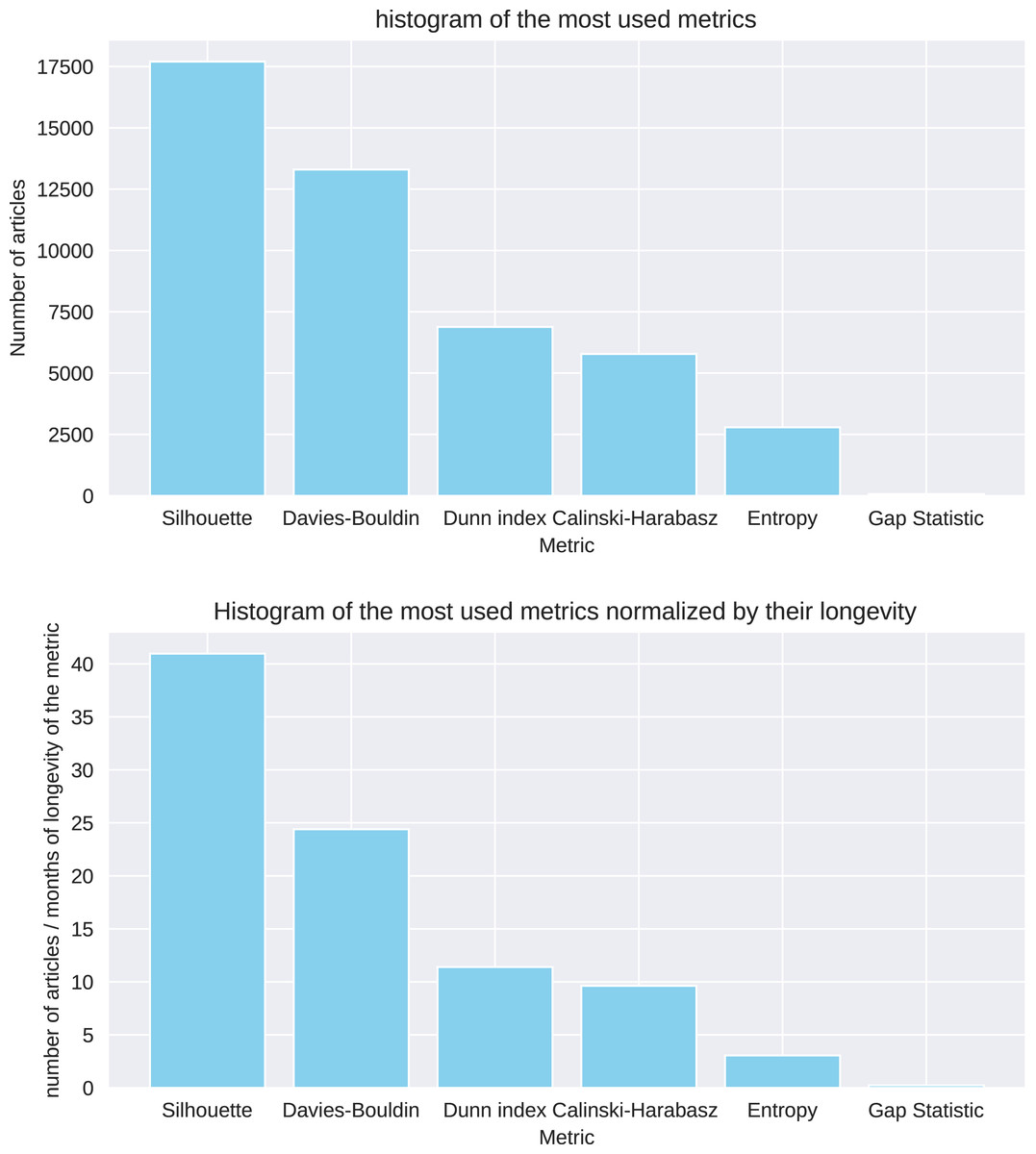
Figure 14: Metrics’ article tallies.
Number of articles citing or using each metric found in Google Scholar in June 2024, including the count since the publication of each original article (Table 17).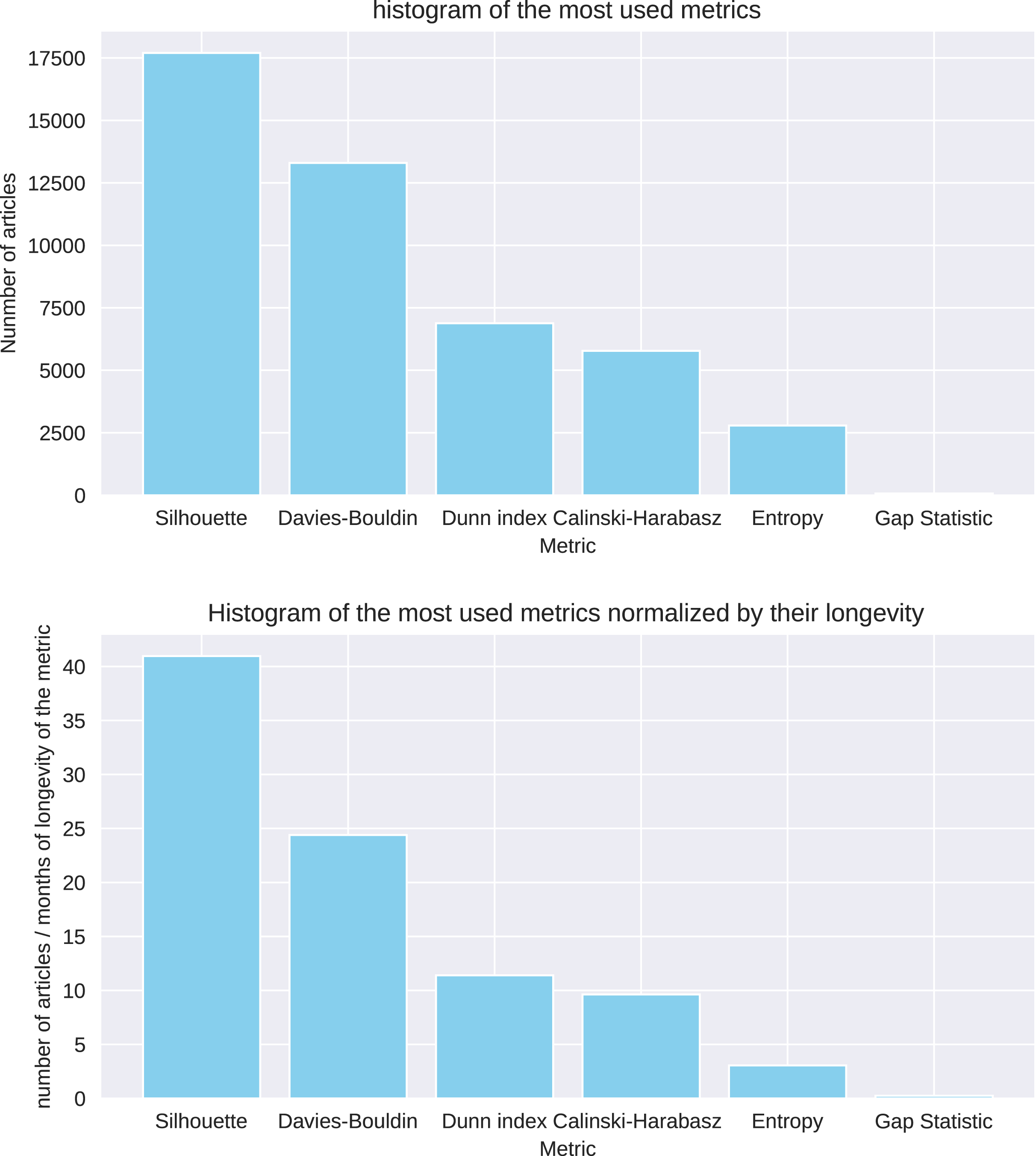
Tests on artificial datasets with a “correct” number of clusters
To further assess the efficiency of the six clustering scores analyzed in this study, we decided to apply them to the results obtained by -means on five public artificial datasets where the number of “correct” convex clusters is known (Thrun & Ultsch, 2020, 2023). We report the results measured by the Silhouette coefficient, Calinski-Harabasz index, reverse Davies-Bouldin index, reverse Shannon entropy, Dunn index, and Gap statistic when the number of clusters varies from 2 to 10. We used the reverse formula of the Davies-Bouldin index and of the Shannon entropy to make all the six coefficients increase when the quality of the clustering result increases: the higher, the better for all the six metrics.
We report the results in Figs. 15, 16, 17, 18, and 19.
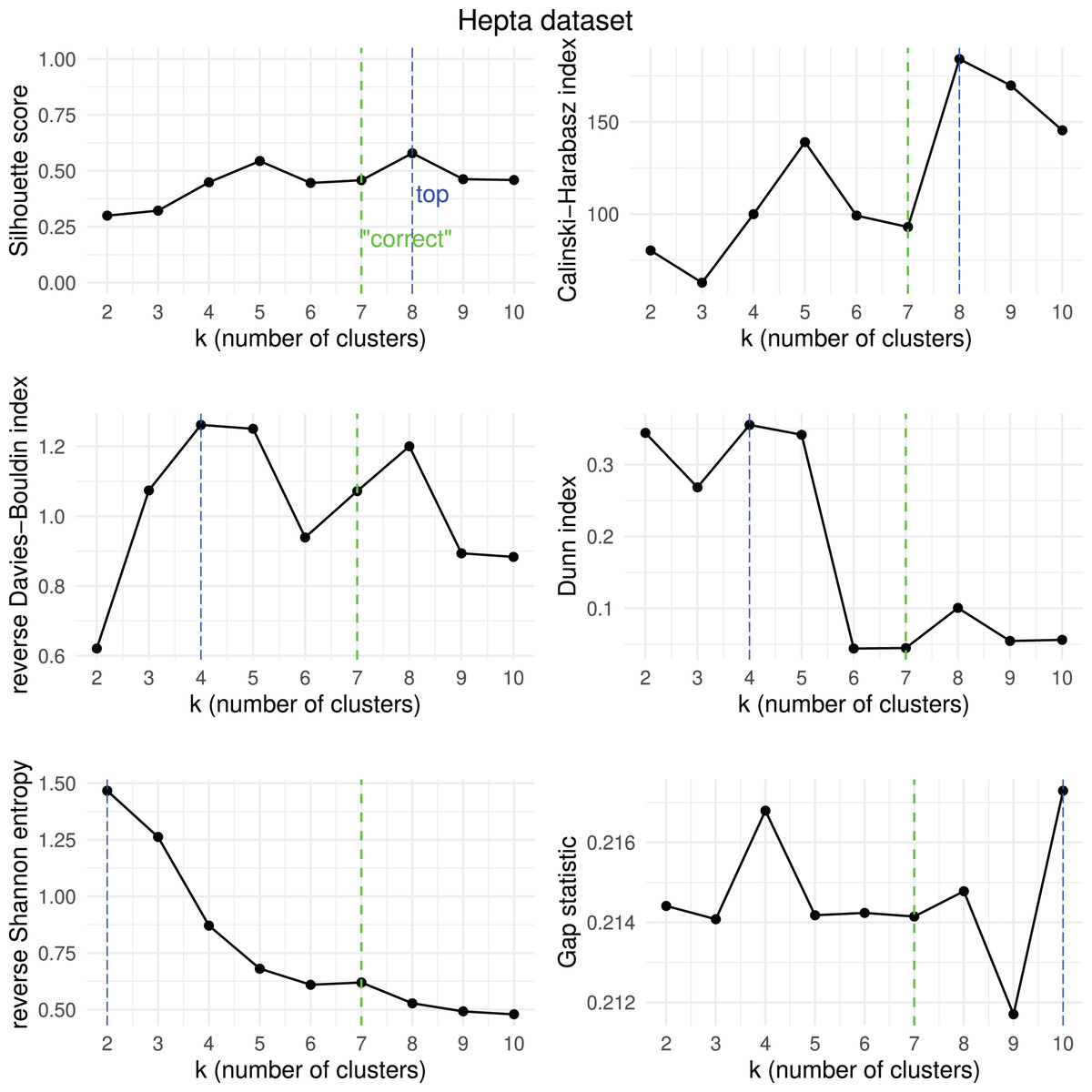
Figure 15: Hepta dataset—results of k-means.
Results obtained by the six clustering internal scores on the outcome of -means on the Hepta dataset when changing the number of clusters from 2 to 10. Green line: the “correct” number of clusters according to the original dataset curators (Thrun & Ultsch, 2020, 2023). Blue line: best result for each metric.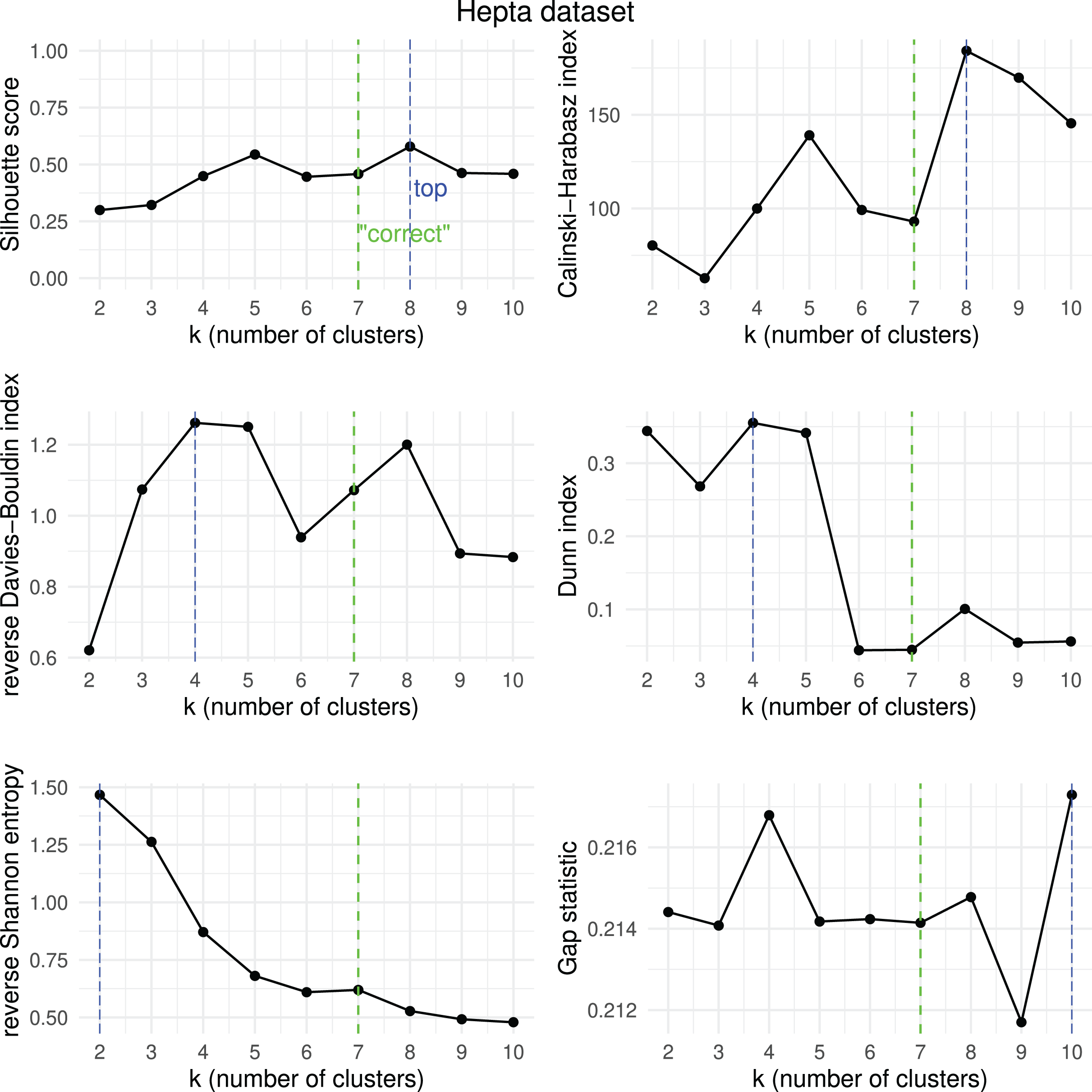
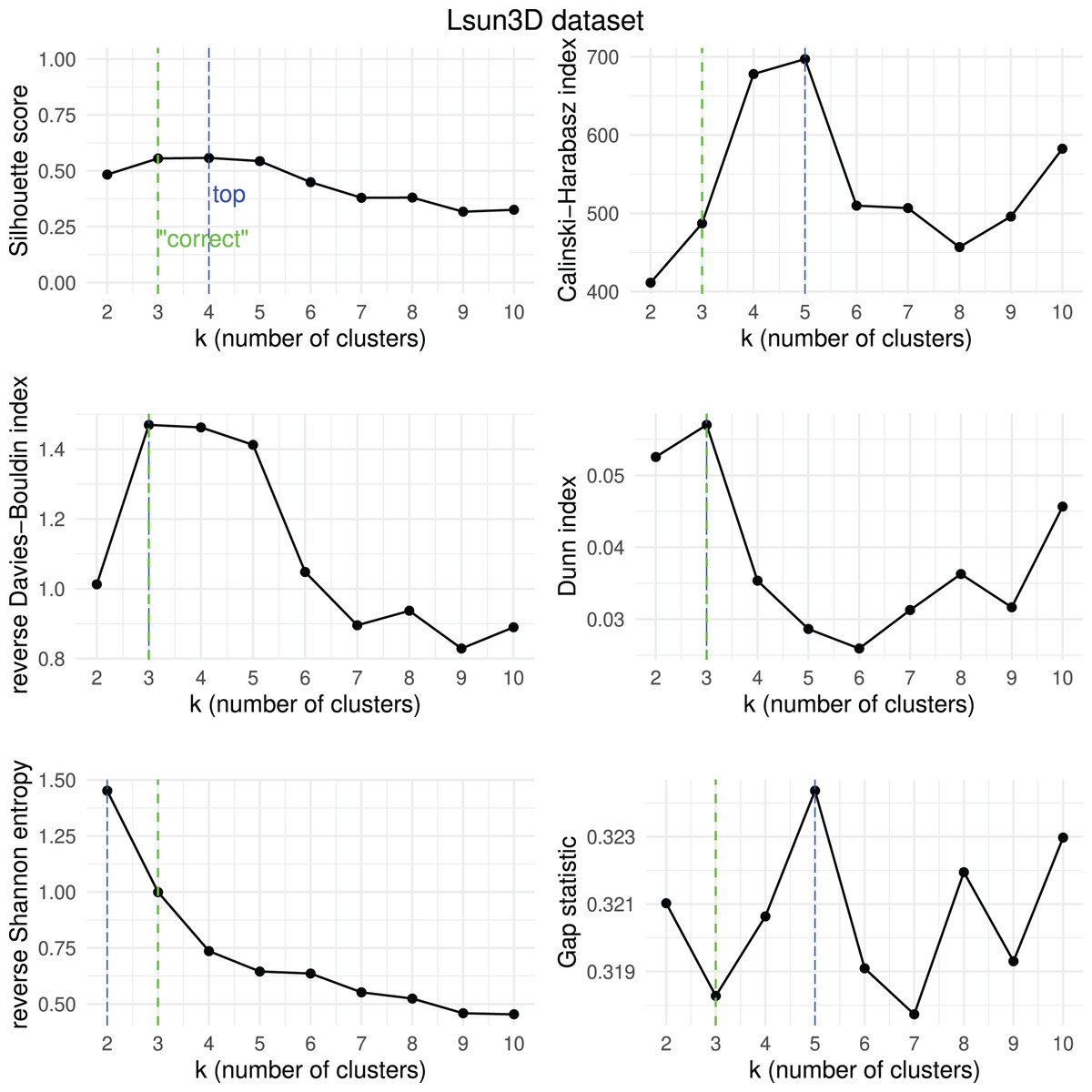
Figure 16: Lsun3D dataset—results of k-means.
Results obtained by the six clustering internal scores on the outcome of -means on the Lsun3D dataset when changing the number of clusters from two to 10. Green line: the “correct” number of clusters according to the original dataset curators (Thrun & Ultsch, 2020, 2023). Blue line: best result for each metric.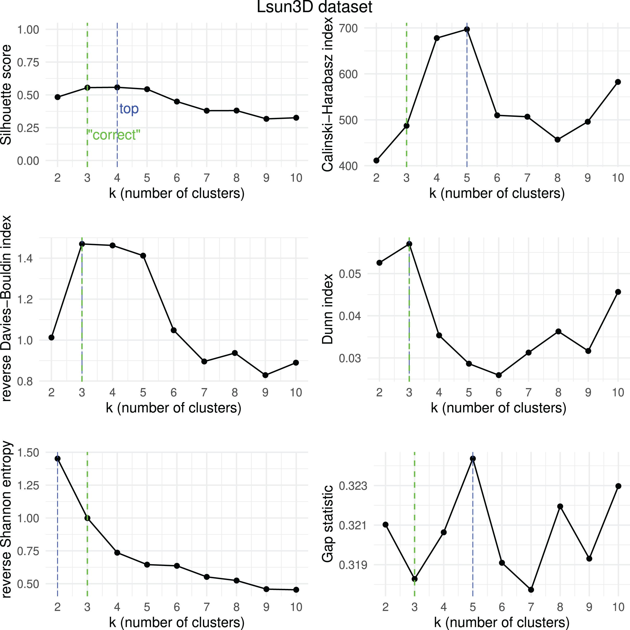
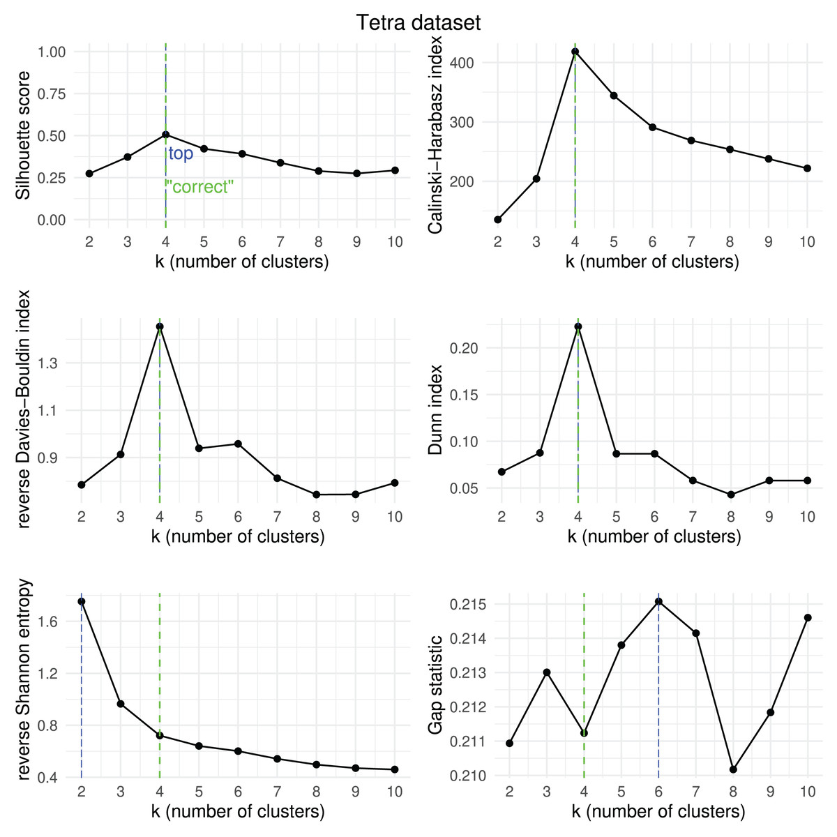
Figure 17: Tetra dataset—results of k-means.
Results obtained by the six clustering internal scores on the outcome of -means on the Tetra dataset when changing the number of clusters from two to 10. Green line: the “correct” number of clusters according to the original dataset curators (Thrun & Ultsch, 2020, 2023). Blue line: best result for each metric.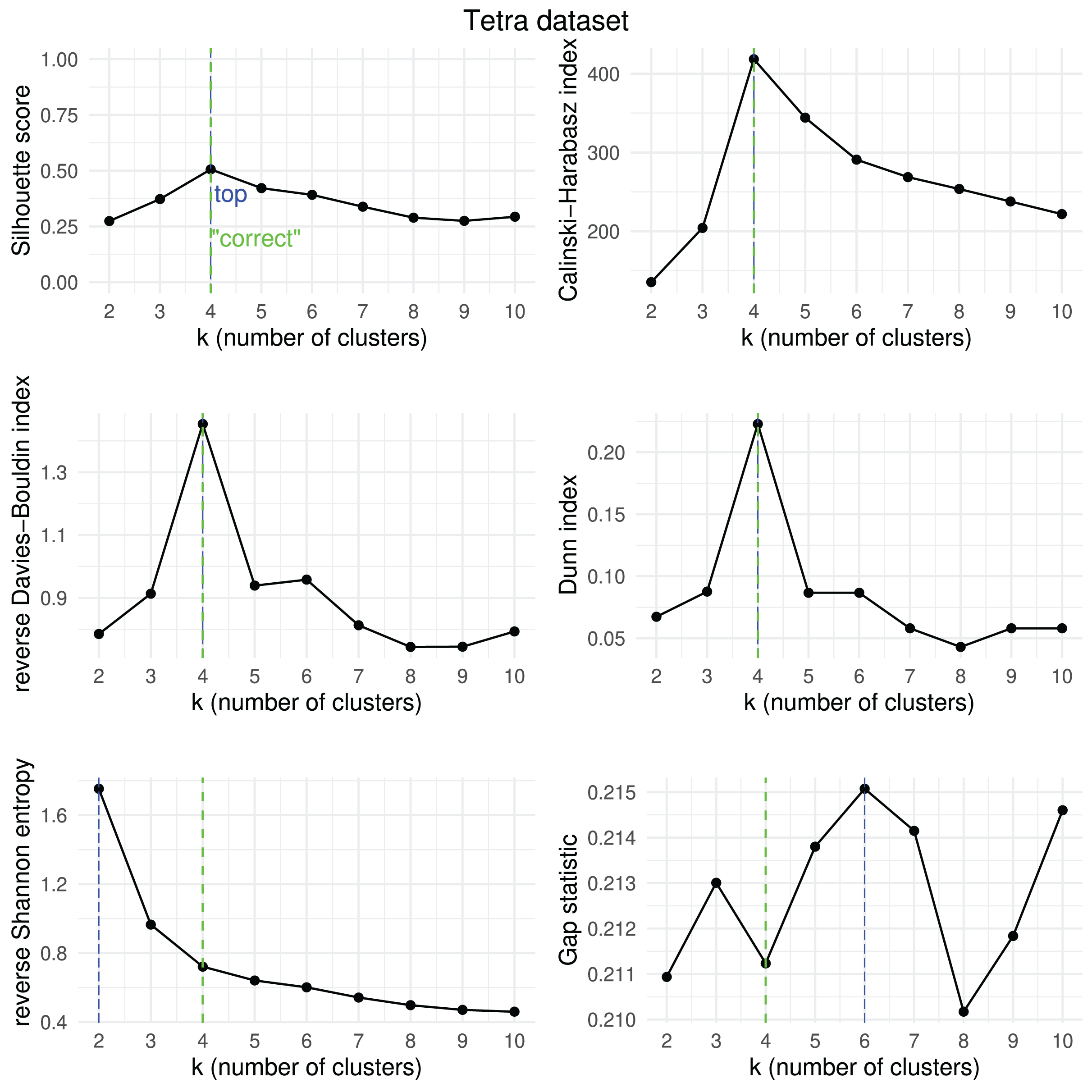
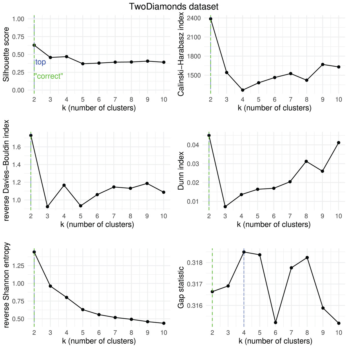
Figure 18: TwoDiamonds dataset—results of k-means.
Results obtained by the six clustering internal scores on the outcome of -means on the TwoDiamonds dataset when changing the number of clusters from two to 10. Green line: the “correct” number of clusters according to the original dataset curators (Thrun & Ultsch, 2020, 2023). Blue line: best result for each metric.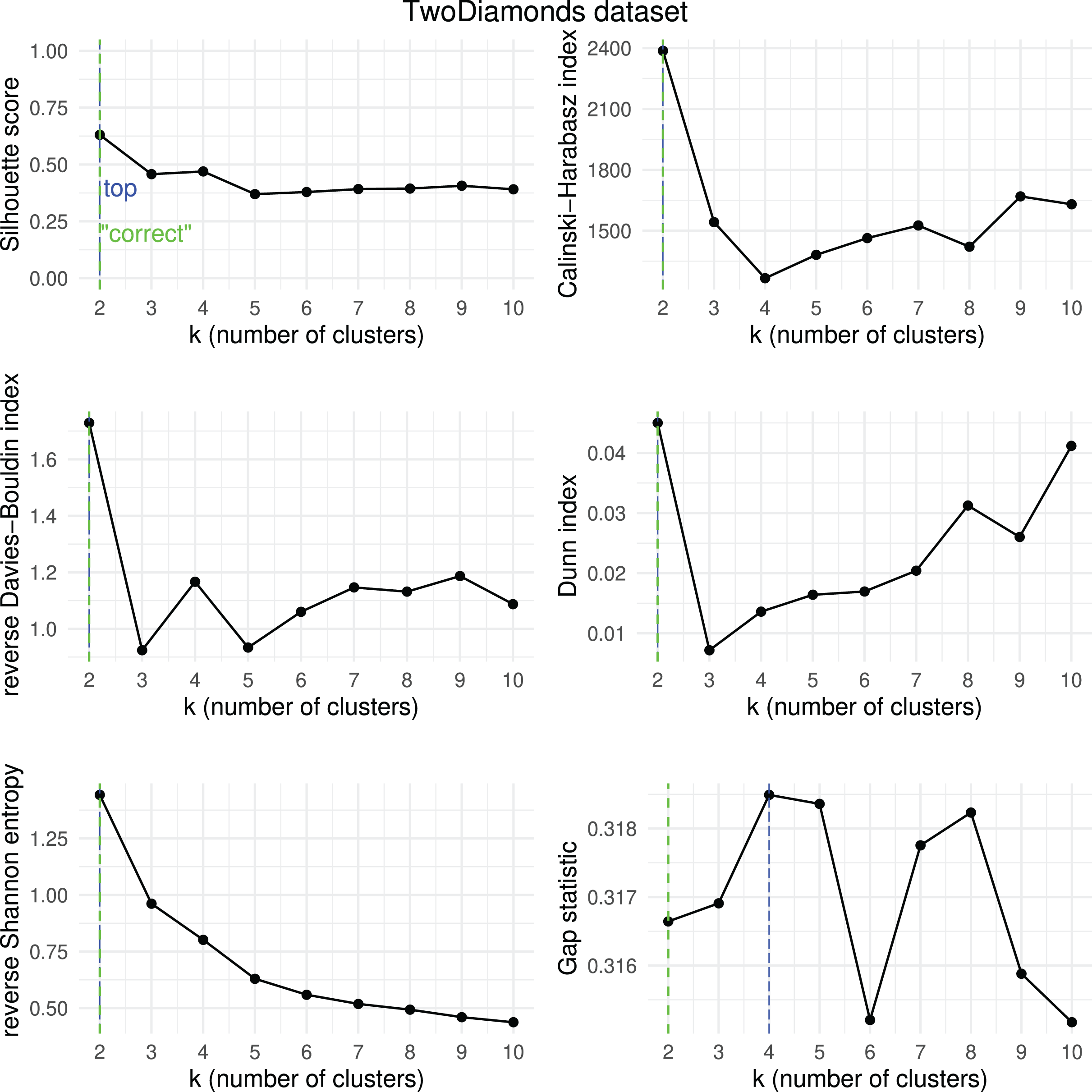
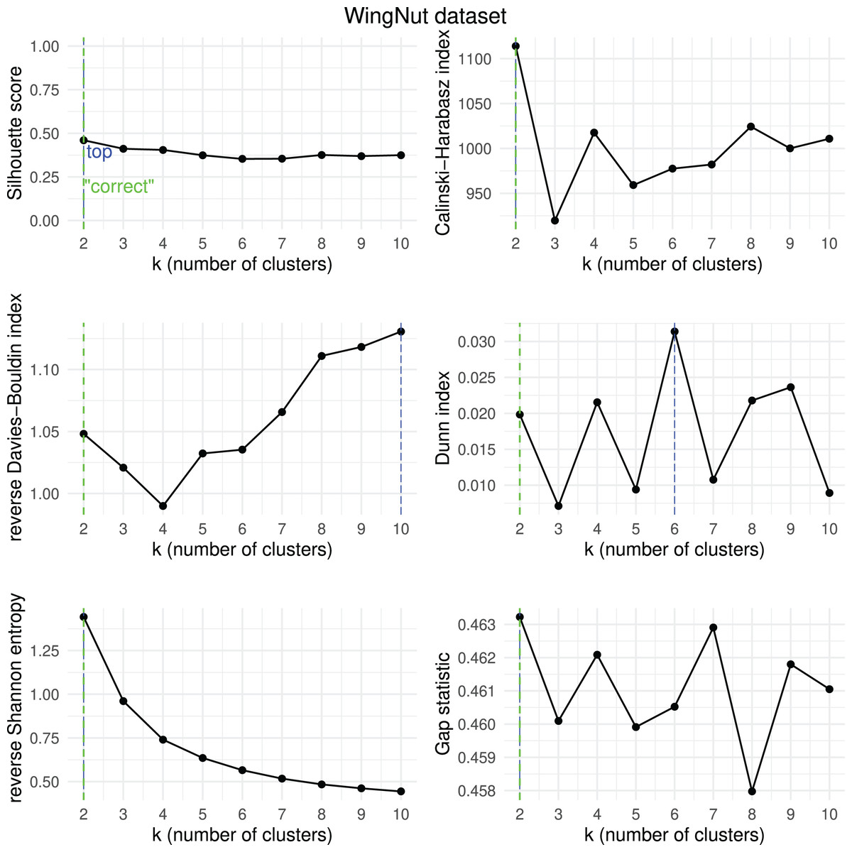
Figure 19: WingNut dataset—results of k-means.
Results obtained by the six clustering internal scores on the outcome of -means on the WingNut dataset when changing the number of clusters from two to 10. Green line: the “correct” number of clusters according to the original dataset curators (Thrun & Ultsch, 2020, 2023). Blue line: best result for each metric.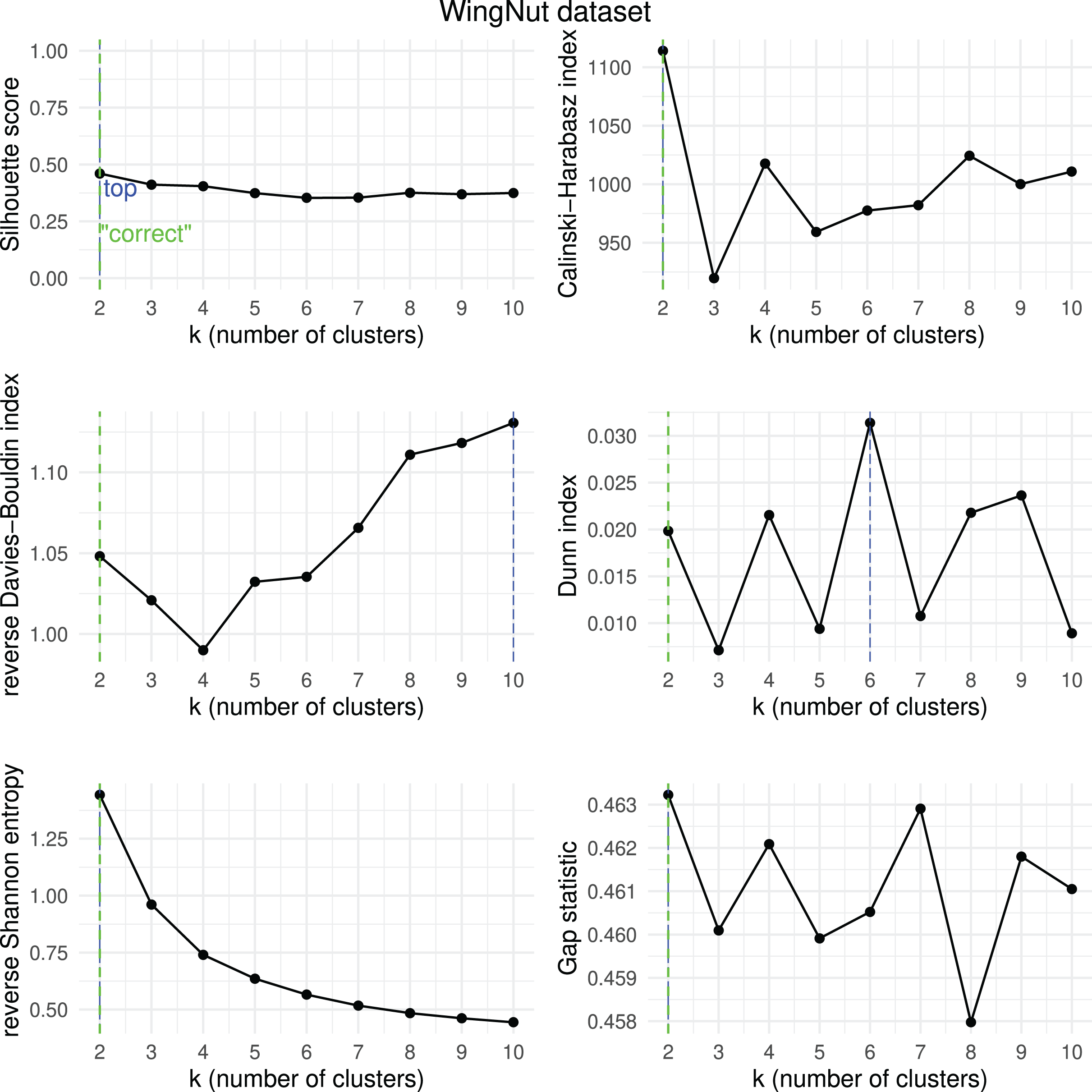
We then checked which metrics had their highest value when corresponding to the “correct” number of clusters, and we recap the results obtained in Table 18. As one can notice, no metric detected the “right” number of clusters in all the five datasets. The Silhouette coefficient, Davies-Bouldin index, Dunn index, and Calinski-Harabasz found the “correct” number of clusters for -means on the majority of cases: three out of five. These tests confirm the higher effectiveness of these three metrics compared to the other ones considered here.
| Ranking | Metric | Consistent trends | |
|---|---|---|---|
| 1 | Silhouette coefficient | 3 out of 5 | 67% |
| 1 | Davies-Bouldin index | 3 out of 5 | 67% |
| 1 | Dunn index | 3 out of 5 | 67% |
| 1 | Calinski-Harabasz index | 3 out of 5 | 67% |
| 4 | Shannon entropy | 2 out of 5 | 40% |
| 6 | Gap statistic | 1 out of 5 | 20% |
Discussion and conclusions
Given the unsupervised nature of clustering, there is no ground truth assess the validity and the reliability of the six metrics for internal clustering assessment. However, in the tests we performed we were able to discover some useful findings:
-
The tests made on the open real-world EHRs datasets highlighted the Silhouette coefficient and Davies-Bouldin index as the two most informative metrics among the six analyzed (real-world medical scenarios).
-
The analysis of the articles mentioning the six analyzed metrics in the scientific literature clearly showed the higher frequency of studies involving the Silhouette coefficient and Davies-Bouldin index (the studied metrics in the scientific literature).
-
The analysis performed through -means on the artificial public datasets featuring a “correct” number of clusters identified the Silhouette coefficient, Davies-Bouldin index, Dunn index, and Calinski-Harabasz index as the most reliable coefficients, even if only on three datasets out of five (tests on artificial datasets with a “correct” number of clusters).
To draw conclusions from these outcomes, we can state that the Silhouette coefficient and Davies-Bouldin index are the most informative, reliable, and effective metrics to use when internally assessing convex-shaped clusters, produced by -means with two clusters, in a Euclidean space. Davies-Bouldin index, however, has a flaw: since its values range from 0 (perfect outcome) to (worst possible outcome) (Table 1), a single value of this metric does not say anything regarding the absolute quality of the clustering results. For example, if one applied a clustering method to a medical dataset and obtained , they would not be able to say if this result is good or bad. They would need to re-execute the test with different hyper-parameters or with a different method, obtain a new value for DBI, and then compare the two. In any case, their results would still be relative to each other. This aspect can have a strong impact on clustering studies; when trying to improve the clustering results in a study, a researcher might wonder when to consider their DBI results sufficient and stop their attempts to improve the computational pipeline. This question might remain unanswered.
The Silhouette coefficient, in contrast, does not have this limitation. As we mentioned at the beginning of this study, the Silhouette coefficient is the only metric among the six studied here which has two finite limits: its values range from (worst possible outcome) to (perfect clustering) (Table 1). This interval means that a single value of Silhouette , for example, indicates an excellent clustering result by itself, without the need to perform a second test for a baseline comparison. The values of Silhouette coefficient, in fact, are absolute and can therefore speak for itself: a researcher obtaining Silhouette in a clustering study can rest assured that their results are optimal. However, the Silhouette coefficient has another flaw, that we mentioned earlier: when the clustering results obtained by -means on the mixed-up, dispersed, and scattered datasets were supposed to be bad, the values of Silhouette still ranged around +0.5 in the interval, inconsistently with the clustering trend. This aspect needs attention: the Silhouette coefficient can be informative when clustering results are good, but it does not seem to be informative when the results are bad. The Davies-Bouldin index, on the contrary, correctly produces the zero value in all the cases where the points are scattered and there are no clear partitions. Therefore, as a key message of this study, we recommend using both the Silhouette coefficient and the Davies-Bouldin index in any clustering study. Our results can have a strong impact on computer science, by potentially influencing many studies involving internal assessment of convex-shaped clustering results, in any scientific field.
Limitations and future developments: We have to say that we studied only the clustering metrics in convex clusters, and we did not explore the evaluation of concave or nested clusters, such as the clusters usually produced by DBSCAN (Schubert et al., 2017) or HDBSCAN (Campello, Moulavi & Sander, 2013). For these cases, the density-based clustering validation (DBCV) index (Moulavi et al., 2014; Chicco, Oneto & Cangelosi, 2025) is one of the possible measures to use. Moreover, we based our study on -means by using only two clusters and the Euclidean distance in all the tests, so we cannot make any claims about the generalizability of our findings for other clustering methods, other numbers of clusters, or other distances. For example, other methods such as hierarchical clustering, mean-shift, or BIRCH might have generated different results. The choice of utilizing the Euclidean distance can also be questioned. For example, as recent study suggests the usage of metrics based on the Minkowski distance, rather than the Euclidean distance, to handle the curse of dimensionality in clustering (Powell, 2022). This aspect can be explored in future studies indeed.
Also, here we focused on the six metrics for internal clustering evaluation that are most commonly used in biomedical informatics, but we know that there are other coefficients for the same scopes that we did not include in this study for space reasons (for example, Wang & Xu, 2019). We utilized six traditional metrics for internal clustering assessment, and we did not consider their enhanced variants, such as the improved Dunn index proposed by Gagolewski, Bartoszuk & Cena (2021): these improved variants of existing metrics can be a topic for a future study. We employed the ARI for the external clustering in the tests on the EHR data, but some might say that other external metrics could have been chosen instead. We are aware of these limitations but we believe that our findings can clearly explain that the Silhouette coefficient and the Davies-Bouldin index are more informative and reliable than the other five metrics studied here for internal clustering evaluation.
We plan to address all these just-mentioned limitations in future studies, especially to explore clustering internal metrics for concave, nested clusters (Moulavi et al., 2014).
Ethics approval and consent to participate: The permissions to collect and analyze the data of patients’ involved in this study were obtained by the original dataset curators (Gucyetmez & Atalan, 2016; Jani et al., 2016; Requena-Morales et al., 2017; Ma et al., 2018; Takashi et al., 2019).