
A hybrid deep learning paradigm integrating segmentation architectures for precise plant disease identification and classification
- Published
- Accepted
- Received
- Academic Editor
- Giovanni Angiulli
- Subject Areas
- Artificial Intelligence, Computer Vision, Data Mining and Machine Learning, Neural Networks
- Keywords
- Deep learning, CNN, Plant disease classification, Image segmentation, Hybrid deep learning models, UNet, DeepLabV3+
- Copyright
- © 2025 Sellappan et al.
- Licence
- This is an open access article distributed under the terms of the Creative Commons Attribution License, which permits unrestricted use, distribution, reproduction and adaptation in any medium and for any purpose provided that it is properly attributed. For attribution, the original author(s), title, publication source (PeerJ Computer Science) and either DOI or URL of the article must be cited.
- Cite this article
- 2025. A hybrid deep learning paradigm integrating segmentation architectures for precise plant disease identification and classification. PeerJ Computer Science 11:e3305 https://doi.org/10.7717/peerj-cs.3305
Abstract
Addressing the challenging issue of complex background interference in plant disease identification, recent research employs diverse deep learning (DL) methodologies on both publicly available and customized datasets. This study introduces a two-step DL approach for plant disease classification. Initially, an enhanced convolutional neural network (CNN) is developed through a comparative analysis of prominent CNN architectures, including customized and cascaded versions of select DL models, achieving an accuracy of 93.3%. To further enhance accuracy, segmentation architectures such as DeepLabV3+, UNet, Iterative UNet, and UNet with Atrous Spatial Pyramid Pooling (ASPP) are integrated before customized CNN architectures. These segmentation algorithms effectively isolate the diseased portions of leaf images. Notably, the UNet with ASPP architecture demonstrates reduced time complexity, minimizing the number of features to be trained, and significantly improves accuracy to 99.8%, outperforming other predefined architectures. The models are trained on a plant village dataset, detecting 10 different diseases across various plant species, including tomato, corn, and potato.
Introduction
Plant diseases deteriorate the quality of plants and it affects the growers of broad-acre crops. The contagious agent in plants can be viral, nematodes, bacterial, or fungal. This can impair the plant parts underneath or over the ground. Finding out the traits of the infected region and knowing when and how to successfully control diseases is an occurring challenge in the agricultural field. Tomato, corn and potato are some of the significant food crops across the globe. It has a per capita utilization of 20 kilograms each year and addresses around 15% of the average total vegetable utilization. Potato and tomato top vegetable choices across countries like the United States of America (USA). China, India, and the USA remain are top consumers of corn. To fulfill the need for these crops it is fundamental to devise methods to work on the yield of tomato, potato and corn and advance early discovery of pests, bacterial, and viral infections. The tomato, potato and corn crops are harvested mainly during the winter and summer seasons. Because of all these environments, plants become exceptionally open to diseases caused by viruses, bacteria, and fungi. Spotting plant disease is one of the significant research topics (Vetal & Khule, 2017).
The rapid transmission of diseases across borders has become more prevalent than ever, adding a layer of complexity to the current situation. Mitigating the harm inflicted by diseases during plant growth underscores the importance of proactive crop disease prevention measures. Recognizing the urgency of this need, there is a compelling call for the implementation of automated image-based tools. In the domain of research, DL (Ferentinos, 2018) shows great promise, especially in improving accuracy compared to traditional machine learning models commonly used for identifying and classifying crop diseases. The notable advancements achieved by DL in computer vision have notably expanded possibilities for early detection of plant diseases, representing a revolutionary stage in agricultural methodologies.
Recent advancements in DL within the field of computer vision have significantly broadened possibilities for the early diagnosis of plant diseases, marking a transformative phase in agricultural practices. While traditional machine learning models have their merits, they encounter challenges in managing the complexity and variability inherent in agricultural datasets, especially those related to plant diseases. Traditional machine learning techniques such as support vector machines (SVM) and random forest classifiers rely heavily on manual feature extraction and often fail to capture the complex spatial patterns present in raw plant images. These methods are typically less accurate and less scalable, especially when applied to large, diverse datasets. In contrast, deep learning models like convolutional neural networks (CNNs) can automatically learn hierarchical features directly from pixel data, making them better suited for handling high variability in disease patterns, lighting conditions, and background noise.
DL in computer vision has significantly advanced the early diagnosis of plant diseases, marking a transformative shift in agricultural practices. While traditional machine learning models have their advantages, they often struggle with the complexity and variability of agricultural datasets. In contrast, DL effectively extracts intricate patterns from images, enabling more accurate disease detection and classification. DL’s adaptability and scalability allow it to be trained on diverse datasets across various crops and diseases, supporting a versatile approach to plant health monitoring. This is especially important given the regional variations in crop diseases worldwide. As agriculture increasingly integrates technological innovations, DL offers a promising path toward sustainable farming by enabling early detection, reducing yield losses, and promoting efficient, targeted disease management.
In recent years, CNN-based DL models have found extensive applications in computer vision, such as medical image recognition (Wang & Liu, 2021; Deng et al., 2022; Czajkowska et al., 2022), expression recognition (Ab Wahab et al., 2021; Liang et al., 2021), traffic detection (Cao, Zhang & Jin, 2021; Li et al., 2021; Liang et al., 2022), text detection (Khan, Sarkar & Mollah, 2021; Boukthir et al., 2022), face recognition, and more. Traditional image classification and recognition methods, as discussed in Liu & Wang (2020), are limited to extracting basic features and struggle with capturing extraordinary and complex image feature data. DL techniques, on the other hand, address and overcome this limitation.
CNN possesses a robust feature extraction capability, which has been leveraged by numerous researchers in prior studies focusing on plant disease prediction methods utilizing DL. This technique has been seamlessly integrated with conventional classifiers. Semantic segmentation method using the U-net model for pest detection (Gutierrez et al., 2019), foliar symptoms (Gonçalves et al., 2021), corn disease detection (Divyanth, Ahmad & Saraswat, 2022), DeepLabV3+ for black gram (Talasila, Rawal & Sethi, 2023), grapes (Shu et al., 2023), apple (Li et al., 2023) disease detections, Iterative UNet and UNet with AtrousSpatial Pyramid Pooling (ASPP) is performed which helps in segmenting the image. The segmented images serve as input for a pre-trained CNN network to obtain features characterizing the images. ResNet for disease detection (Sravan et al., 2021) and facial expression (Li & Lima, 2021) is a new neural architecture for reducing complexity, which allows us to train extremely deep neural networks. It allows us to solve the degradation problem while keeping good performance. By reducing complexity, a smaller number of parameters need to be trained and less time on training as well. AlexNet is one of the leading architectures that can be used for object detection (Pal et al., 2021) and has been applied to many artificial intelligence problems. In addition to pre-trained models a customized model was constructed with convolutional pooling layers and batch normalization.
The results of the experiments undeniably illustrate the efficacy of the segmentation, feature extraction, and concatenation processes employed in the models proposed. To succinctly capture the noteworthy contributions, it is delineated as follows:
Image segmentation
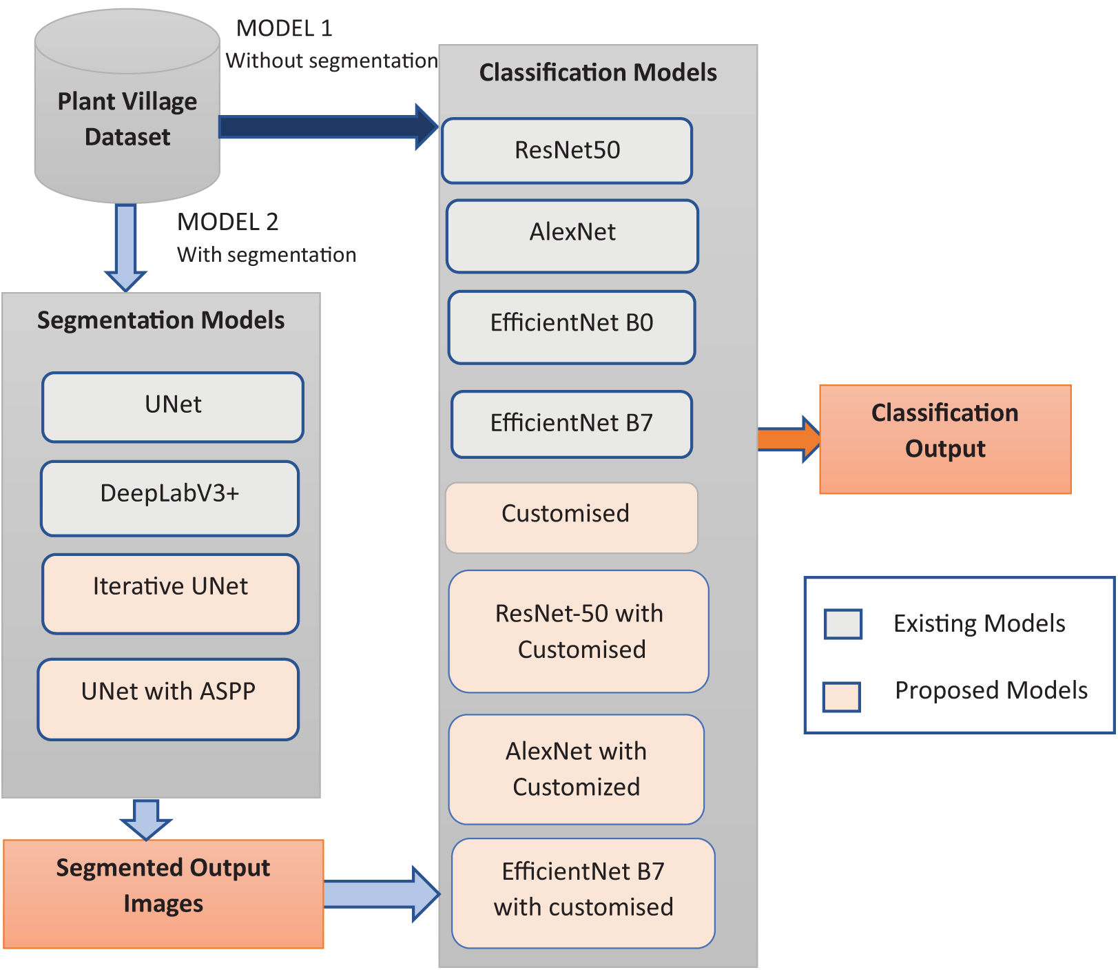
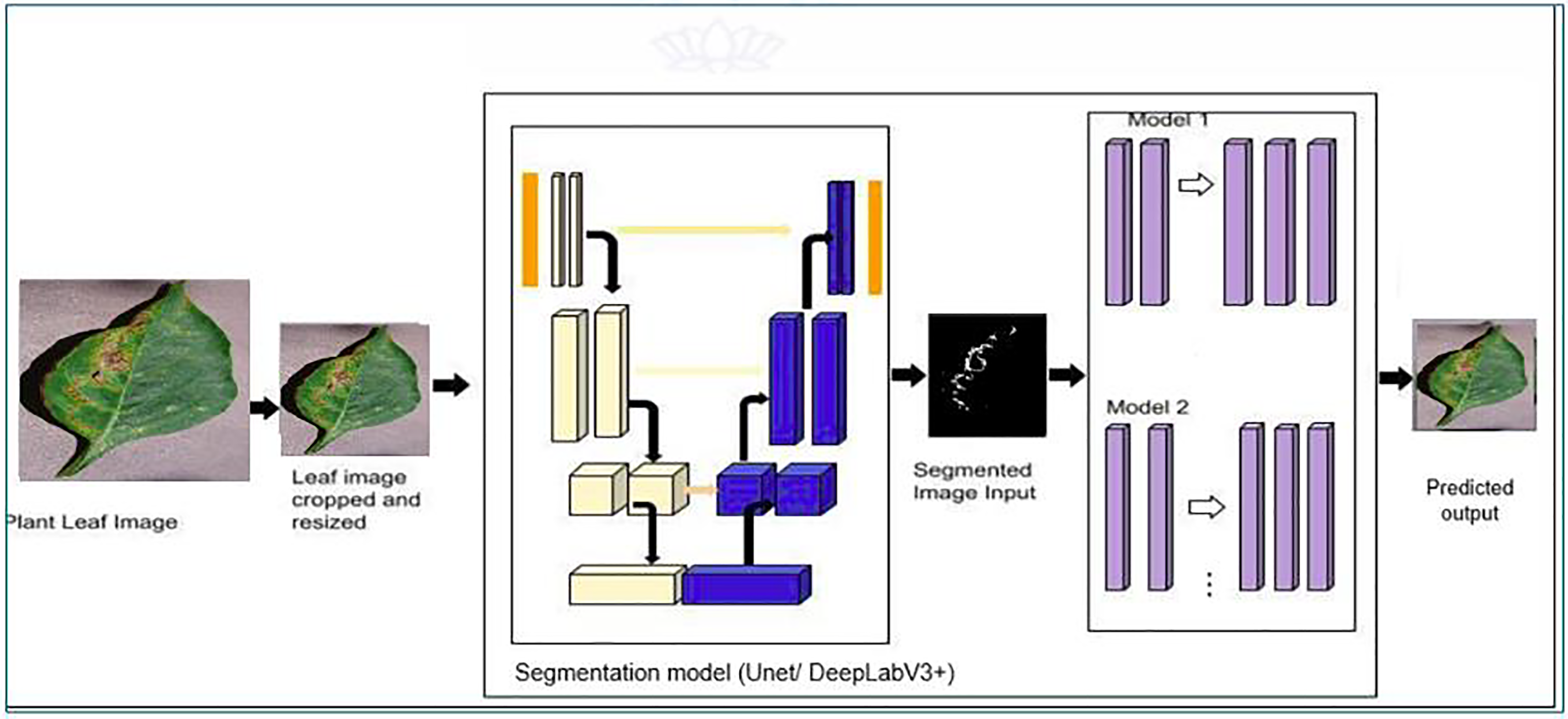
The proposed study introduces two innovative architectures, namely Iterative UNet and UNet with ASPP module, as depicted in Fig. 1. These novel approaches are systematically compared against established predefined segmentation models, thereby showcasing the superiority of the proposed methods in the domain of image segmentation. The results underscore the efficacy of the segmentation techniques in accurately delineating and isolating diseased regions within leaf images.
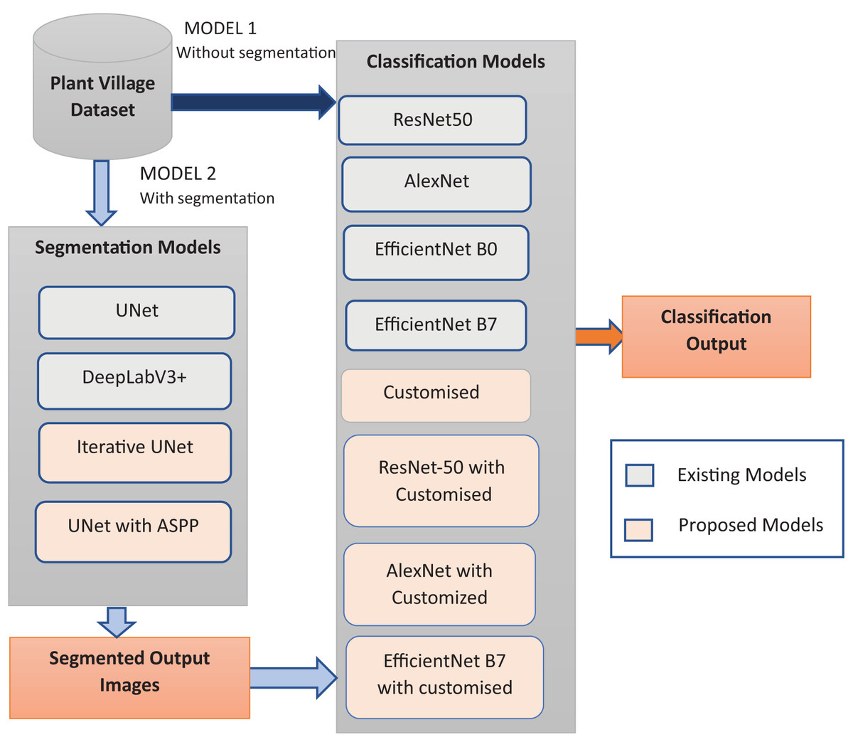
Figure 1: Proposed workflow.
Feature extraction
The feature extraction phase is meticulously executed using the uniquely devised customized architectures, complemented by a hybrid approach that involves the concatenation of both customized and predefined models, as illustrated in Fig. 1. This methodical comparison extends to well-established architectures, offering a comprehensive understanding of the enhanced capabilities of the proposed models in extracting pertinent features. The dual-pronged approach not only underscores the effectiveness of the customization but also accentuates the synergistic benefits derived from the amalgamation of novel and established elements in feature extraction. The proposed models excel in capturing and representing distinctive features critical for accurate plant disease classification. The conducted comparative analyses validate the superiority of the proposed approaches, confirming their potential to substantially improve the accuracy and efficiency of plant disease identification systems.
The results of the experiments undeniably illustrate the efficacy of the segmentation, feature extraction, and concatenation processes employed in the models proposed. To succinctly capture the noteworthy contributions, it is delineated as follows:
The study introduces two novel segmentation architectures—Iterative UNet and UNet with ASPP module—to enhance the accuracy of diseased region identification in plant leaf images. These architectures are systematically compared with established segmentation models, demonstrating their superior performance in delineating and isolating affected areas.
A unique feature extraction methodology is proposed, integrating customized architectures with predefined models to enhance feature representation. The hybrid approach ensures the extraction of highly discriminative features, leading to improved classification accuracy in plant disease identification.
To optimize computational resources, weight-based pruning techniques are incorporated into the proposed architectures. This enhances the efficiency of the models by reducing computational complexity while maintaining segmentation and classification accuracy, making the approach feasible for real-time agricultural applications.
The study highlights the practical implications of the proposed methodologies by evaluating their performance across various plant disease datasets, ensuring robustness and adaptability in real-world agricultural scenarios.
The following section describes the literature survey of various works handled in this area. ‘Materials & Methods’ describes the materials and methods used. ‘Results’ goes through with the result and discussion part. Whereas ‘Discussion’ compares the proposed work with the existing state-of-the-art methods and finally ‘Conclusions’ discusses the conclusion and future scope.
Motivation
The growth prevalence of plant diseases have significant challenges to global agriculture, as they degrade the quality and yield of essential crops and have a high impact growers. Viral, bacterial, fungal, and nematode infections compromise various plant parts, often hindering growth and productivity. Among the most widely consumed crops—tomato, potato, and corn—disease outbreaks have substantial socio-economic implications. These crops account for a significant share of global food consumption, with per capita utilization exceeding 20 kilograms annually for tomatoes alone, while potatoes and corn hold pivotal roles in the diets of countries like the USA, China, and India.
The seasonal nature of these crops exposes them to a range of pathogens, necessitating robust, timely interventions to mitigate losses. Early identification of diseases is critical in reducing yield loss and ensuring sustainable farming practices. Traditional methods for diagnosing plant diseases often rely on manual inspection, which is both time-consuming and prone to inaccuracies due to the complexity and variability of symptoms. The rapid globalization of trade has further exacerbated the risk of cross-border disease transmission, adding urgency to the need for innovative, scalable solutions.
In this context, DL emerges as a transformative tool, offering unprecedented accuracy and efficiency in disease detection and classification. By leveraging advanced CNNs, DL models can autonomously analyze intricate patterns in plant images, enabling precise identification of diseases. These advancements in computer vision have revolutionized agricultural methodologies, paving the way for automated, image-based tools that enhance early disease detection capabilities.
Moreover, DL’s adaptability allows it to train on diverse datasets encompassing various crops and diseases, making it a versatile and scalable solution for addressing global agricultural challenges. Beyond mitigating yield losses, DL-driven disease detection aligns with sustainable agricultural practices by enabling targeted interventions and resource-efficient disease management strategies. This research underscores the potential of DL to not only transform plant disease diagnostics but also contribute to the broader goal of ensuring food security in an increasingly complex agricultural landscape.
Materials AND methods
Computing infrastructure: Experiments were carried out using an Intel(R) Core (TM) i7-113H processor, which processes at 3.30 GHz and comprises 4 Core(s). The system’s Random Access Memory is 16 GB, with a graphics processing unit of 4 GB. The latest version of Python, 3.12.3, is used to implement the algorithms. TensorFlow and Keras frameworks were used to implement the baseline classifier algorithms.
3rd party dataset DOI/URL: The dataset used in this research can be accessed using the link given: https://gitlab.com/huix/leaf-disease-plant-village.
Evaluation method: The evaluation consists of several experiments aimed at comparing different models and techniques for plant disease classification and image segmentation using the PlantVillage dataset. The first experiment compares the performance of ResNet50, AlexNet, EfficientNet B0, EfficientNet B7, customized models, and hybrid models on non-segmented images. The EfficientNet-based tailored model achieves superior accuracy and lower loss, while the customized model demonstrates improved accuracy and reduced inference time. In the second experiment, image segmentation performance is evaluated using UNet, DeeplabV3+, Iterative UNet, and UNet with ASPP. UNet performs well with its encoder-decoder structure, while Iterative UNet and UNet with ASPP outperform traditional methods by refining segmentation and capturing contextual information at multiple scales.
Further experiments compared segmented images using UNet with ASPP with different classification models, with Hybrid EfficientNet B7 with Customized Model providing the best accuracy. However, the customized model achieved similar accuracy with reduced time complexity. The fourth experiment explored the effect of different optimizers, with the Adam optimizer providing the best accuracy and lowest loss. In the final testing phase, 20 images from 10 distinct classes were tested, yielding a 97% accuracy, with ResNet50 achieving the highest success rate. The experiments collectively analyzed the performance of both non-segmented and segmented images, demonstrating the advantages of using UNet with ASPP for segmentation and customized models for classification. Graphical representations of the model performances are shown in graphs illustrating training curves and segmentation improvements.
Literature survey
Soulami et al. (2021) introduced a UNet model designed to identify, segment, and predict breast cancer. The segmentation and classification achieved an intersection over union (IOU) score of 90.5%, and the curve reached 99.88% when applied to Digital Database for Screening Mammography (DDSM) and INbreast datasets. The technique involved classifying every pixel in mammogram images. The utilized datasets encompassed a DDSM, a Curated Breast Imaging Subset of DDSM (CBIS-DDSM), and INbreast (Soulami et al., 2021).
Xiong et al. (2020) proposed an algorithm to introduce a detection technique for cash crop diseases. In order to detach the image background without human intervention an automatic image segmentation algorithm that uses the GrabCut algorithm is used but it retains the disease spots in cash crops. It was able to give a maximum recognition rate of over 80% for the 27 diseases (Xiong et al., 2020). The background of the infected regions is separated by the coefficient-based segmentation which was proposed by Khan et al. (2018). Then VGG16 and caffeAlexNet pre-trained models were used to extract features from chosen disorders. To fuse the extracted features before the max-pooling stage, a parallel features fusion step is integrated. Before using multi-class SVM, the majority of univariant characteristics are selected using genetic algorithms. Openly available datasets such as- plant village and CASC-IFW are used for experiments to reach the 98.60% classification accuracy target.
In a study conducted by Daniya & Vigneshwari (2021) they employed segmentation techniques using the Segmentation Network (SegNet). The integration of statistical, CNN, and texture features was a key facet of their methodology. These distinctive features, when harnessed within the framework of deep recurrent neural networks (RNN), were utilized for predictive modeling of plant diseases. To optimize the Deep RNN’s performance, the researchers employed the RideSpiderWater Wave (RSW) algorithm during the training phase. It gave an accuracy rate of 90.5%. This underscores not only the efficacy of the Deep RNN approach but also highlights the superior performance facilitated by the synergistic integration of SegNet segmentation, statistical, CNN, and Texture features, all guided by the innovative RSW algorithm (Daniya & Vigneshwari, 2021).
Chen et al. (2021) proposed a new method for BLS and rice leaf lesion detection. The segmentation was performed using the UNet network. In order to improve the precision of lesion segmentation, BLSNet used a consideration mechanism and multi-scale extraction integration. The proposed BLSNet model demonstrated higher segmentation and class accuracy, with a score of 98.2% (Chen et al., 2021). Rahman et al. (2019) and his research team executed a sophisticated segmentation approach, incorporating a sequential application of thresholding and morphological operations. To bolster the classification process, they employed a deep neural network. The noteworthy outcome of this research was a remarkable accuracy rate of 99.25%. It is crucial to highlight that their study relied on the comprehensive PlantVillage dataset (Rahman et al., 2019), emphasizing the robustness and reliability of their findings within the context of plant disease diagnosis and classification.
Altuntaş & Kocamaz (2021) introduced a method for deep feature extraction to identify tomato leaf diseases. Established pre-trained models like AlexNet, GoogLeNet, and ResNet-50 were employed as feature extractors. The deep features extracted from these models were combined to enhance prediction performance. The SVM classifier underwent training using 1,000 deep features obtained from the final fully connected layers of the CNN models. The accuracy rating for these combined deep features was 96.99%. The PlantVillage Dataset was used (Altuntaş & Kocamaz, 2021). For feature extraction using PlantVillage, Mohameth, Bingcai & Sada (2020), assessed the CNN models have to do with transfer learning and deep feature extraction. Three different CNN models were utilized, for example, ResNet 50, Google Net and VGG-16 two unique classifiers SVM and KNN (Mohameth, Bingcai & Sada, 2020).
ResNet is a well-known pre-trained CNN architecture, Kumar et al. (2020), worked on an open dataset which consists of 15,200 crop leaves images to perform a task of feature extraction and classification using ResNet34 model. The proposed model achieved a 99.40% accuracy on a test set. Subramanian, Shanmugavadivel & Nandhini (2022) utilized several pre-trained models to extract features and classify corn leaf diseases. The application of these trained models resulted in an accuracy of 93% in the classification of corn leaf diseases. The PlantVillage Dataset (Subramanian, Shanmugavadivel & Nandhini, 2022) was employed for this purpose.
Mobeen-ur-Rehman et al. (2019) implemented the computerized tools to recognize diabetic retinopathy. They have used CNN models that are pre-trained specifically AlexNet, SqueezeNet and VGG16 for classification that gives the accuracy of 93.46%, 91.82% and 94.49% discreetly. Additionally, a modified CNN model with five layers, two convolutional layers and three fully linked layers is suggested. Sensitivity, accuracy, and specificity for this approach were optimistic, with values of 98.94%, 97.87%, and 98.15%, respectively. They used the MESSIDOR Dataset (Mobeen-ur-Rehman et al., 2019). Verma, Chug & Singh (2020), have carried out three pretrained models for detecting severity of tomato late blight disease. The tomato late blight leaf images were taken from Plant Village data set based on three categories of severity namely- early, middle and end. The AlexNet, InceptionV3 and SqeezeNet pre-trained models were used for extracting features and extracted features were used for training multiclass SVM. In the proposed work AlexNet was able to perform well with highest accuracy of 93.4% (Verma, Chug & Singh, 2020).
Wang et al. (2021), suggested a two-stage model for cucumber leaf disease severity classification (DUNet) on complicated backdrops that merges DeepLabV3+ and U-Net. The DeepLabV3+ Model first segments the complicated backgrounds. The images are utilised as the input for the second step after the background has been segmented. UNet is employed for the segmentation in the second stage. It has a Dice coefficient of 0.6914 and a 93.27% accuracy rate. The average disease severity accuracy has been 92.85% (Wang et al., 2021).
Alotaibi & Alotaibi (2020) implemented hybrid architecture by combining Inception and Resnet architectures for hyperspectral image classification (HSI). Four standard HSI datasets were utilised to test the model. The proposed model was expert to achieve the highest of 99.02% accuracy on the Pavia Centre scenes dataset (Alotaibi & Alotaibi, 2020). The classification accuracy largely relies on depth of network and so Li et al. (2019), made a deep feature fusion model which uses pre-trained ResNet50 and VGG16 models to extract features. In the proposed work they made use of the UC Merced land-use dataset with 21 classifications and NWPU-RESISC45 dataset with 45 scene classes. The model was able to attain 99.31% with UCMD dataset and has obtained 94.03% with NWPU45 dataset (Li et al., 2019).
In order to tackle the issue of varying size of maize disease, Yang, Shan & Qu (2020) introduces an enhanced segmentation network model called Deeplabv3+. The proposed model addresses the problem through two main stages. Firstly, in the encoding stage, Resnet101 with atrous convolution is employed for feature extraction, along with the inclusion of the Jump-Connected Atrous Spatial Pyramid Pooling (JCASPP) module. This combination allows for the acquisition of multi-scale semantic information. Secondly, in the decoding stage, the output of JCASPP is merged with the shallow features of the backbone network. This integration facilitates the enrichment of spatial information through the utilization of multilayer and small multiplicative up sampling techniques.
In Mandal (2023) discussed recent advancements and challenges in the field of plant leaf disease detection. Utilizing advanced imaging methods and DL, the survey aims to provide a valuable reference for researchers involved in plant disease detection. It presents cutting-edge models to optimize the detection process, reducing time and costs. Additionally, the article explores existing challenges in the detection process, emphasizing the importance of finding solutions.
The above literature survey clearly portraits the different researches happened towards plant disease detection with various CNN architectures and algorithms. The main drawbacks discussed are the heavy model architectures and the enormous features accumulated for image processing. So in this work the heavy models are replaced with a light weight customized model along with hybrid UNet and DeepLabV3+ segmentation to reduce the total trainable parameters.
Proposed model
The proposed model’s classification architecture diagram is displayed in Fig. 2. in which the images from the dataset are cropped and resized and fed to the pretrained models and proposed hybrid models for classification. The architectural configuration of the proposed model for classification, incorporating segmentation, is visually depicted in Fig. 3. In this schematic representation, images sourced from the dataset undergo a sequence of preprocessing steps, including cropping and resizing.
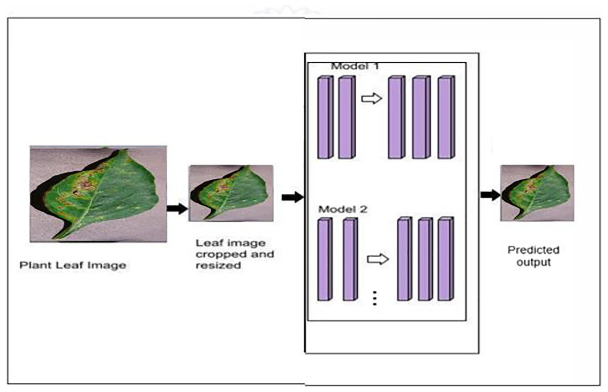
Figure 2: Proposed classification architecture without segmentation—MODEL 1.
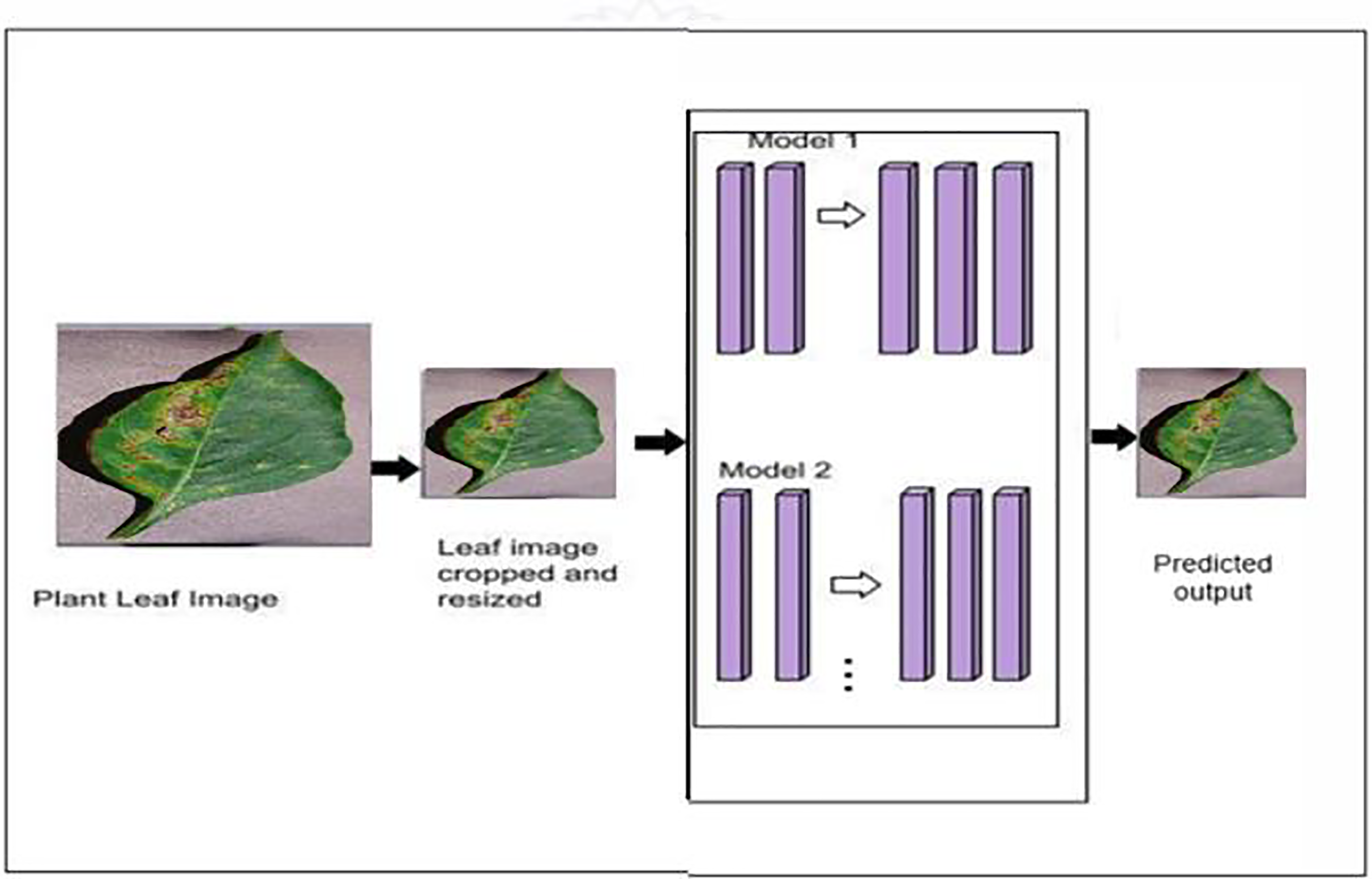
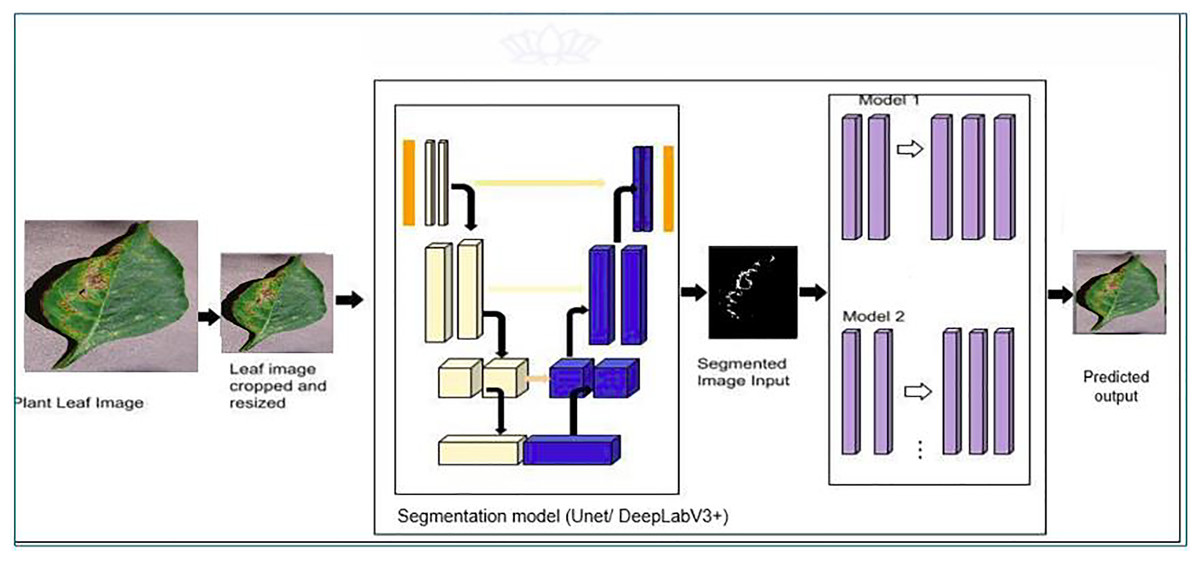
Figure 3: Proposed classification architecture with segmentation—MODEL 2.
Subsequently, these preprocessed images are input into a series of models, namely UNet, iterative UNet, UNet with ASPP, and DeepLab V3+, each dedicated to segmentation tasks. The process entails leveraging both pretrained models and the innovative hybrid models introduced in the proposal for extracting features crucial to the classification process. This amalgamation of established architectures and novel, custom-designed models enhances the robustness and versatility of the overall system, thereby contributing to the efficacy of classification and segmentation tasks within the proposed framework.
Dataset description
For the task of plant leaf disease detection, this study primarily focuses on three widely cultivated crops: tomato, potato, and corn. The leaf images utilized are sourced from the well-established and publicly available PlantVillage dataset, known for its high-quality, labeled images. Table 1 provides a detailed summary of the plant leaf diseases considered, along with the corresponding number of images per class included in the dataset.
| Diseases | Images |
|---|---|
| Corn cercospora leaf spot/gray leaf spot | 513 |
| Corn common rust | 1,192 |
| Corn northern leaf blight | 985 |
| Corn healthy | 1,162 |
| Potato early blight | 1,000 |
| Potato late blight | 1,000 |
| Potato healthy | 152 |
| Tomato bacterial_spot | 2,127 |
| Tomato yellow_leaf_curl_virus | 5,357 |
| Tomato healthy | 1,591 |
| Total | 15,079 |
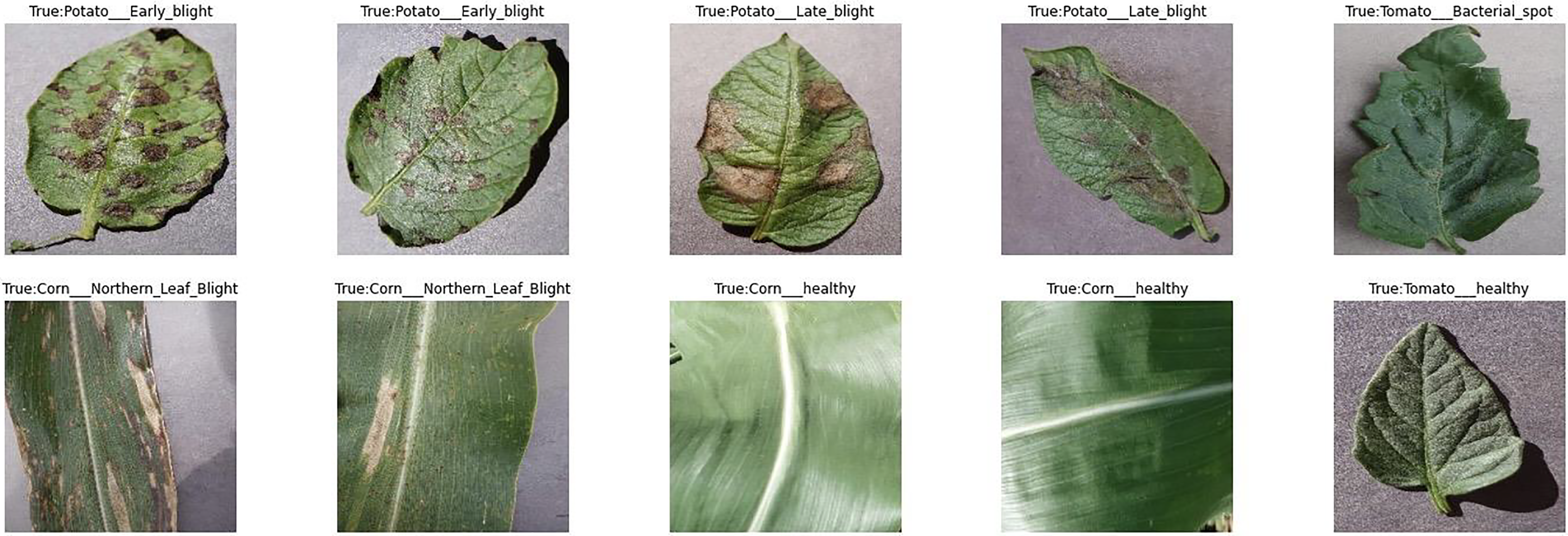
A comprehensive visual overview is presented in Fig. 4, which displays representative samples encompassing both healthy and diseased leaves from the selected crops. The dataset comprises a substantial collection of 15,079 images, reflecting a diverse array of leaf conditions and disease manifestations across the three crop types. These images are categorized into 10 distinct classes, capturing the variations in disease symptoms and healthy foliage with precision.
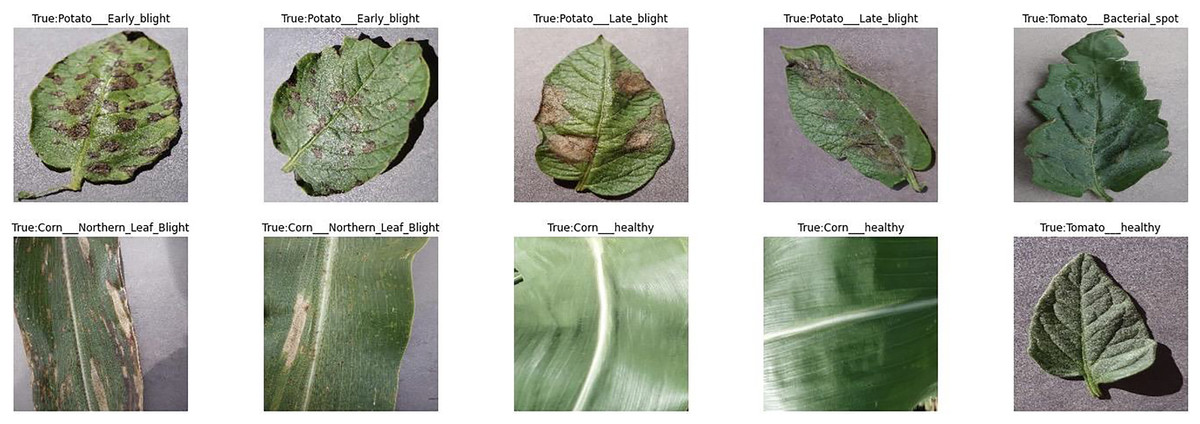
Figure 4: Plant village dataset sample images.
To ensure effective model training and evaluation, the dataset is systematically partitioned. A majority portion, 13,554 images, is allocated for training, providing the deep learning model with a rich and varied learning base. An additional 1,505 images are reserved for validation, allowing for fine-tuning of model parameters and performance optimization during training. For model evaluation, a concise yet critical test set of 20 images is designated to assess the model’s generalization ability on unseen data.
This deliberate and structured data allocation reflects a methodical and performance-driven approach, aimed at enhancing the model’s accuracy, robustness, and reliability in detecting plant leaf diseases across multiple crop species under diverse conditions.
Pre-processing
Image pre-processing plays a crucial role in transforming the raw dataset into a format suitable for network analysis. Given that images in the dataset vary in size and come from different sources, including those with noisy backgrounds, the initial step involves resizing them to a standardized dimension. To achieve this, a resizing function is employed, ensuring that 256 × 256-pixel square images are effectively transformed into 224 × 224-pixel square images. This process carefully maintains the aspect ratios of the images while utilizing zero padding, a strategy that aligns with the model’s requirements and contributes to improved results.
Proposed semantic segmentation
Semantic segmentation involves assigning a class label to each pixel in an image, distinguishing it from classification, where a single class is assigned to the entire image. In semantic segmentation, instances of the same class are treated as individual objects, while instance segmentation considers different instances of a similar class as distinct items. Following preprocessing, the image undergoes segmentation, dividing it into segments with similar intensities and similarities. Subsequently, the image enters the Hue Saturation and Intensity (HIS) model. Semantic segmentation is executed using the U-net architecture, an extension of CNN with some modifications. This sophisticated model effectively addresses existing challenges, demonstrating faster image segmentation capabilities, processing images of size 512 × 512 within seconds. In reference to Badrinarayanan, Kendall & Cipolla (2017), images pass through an encoder where spatial information decreases and feature information increases, followed by the same passing through a decoder. Post-segmentation, the images are subjected to a CNN model for feature extraction.
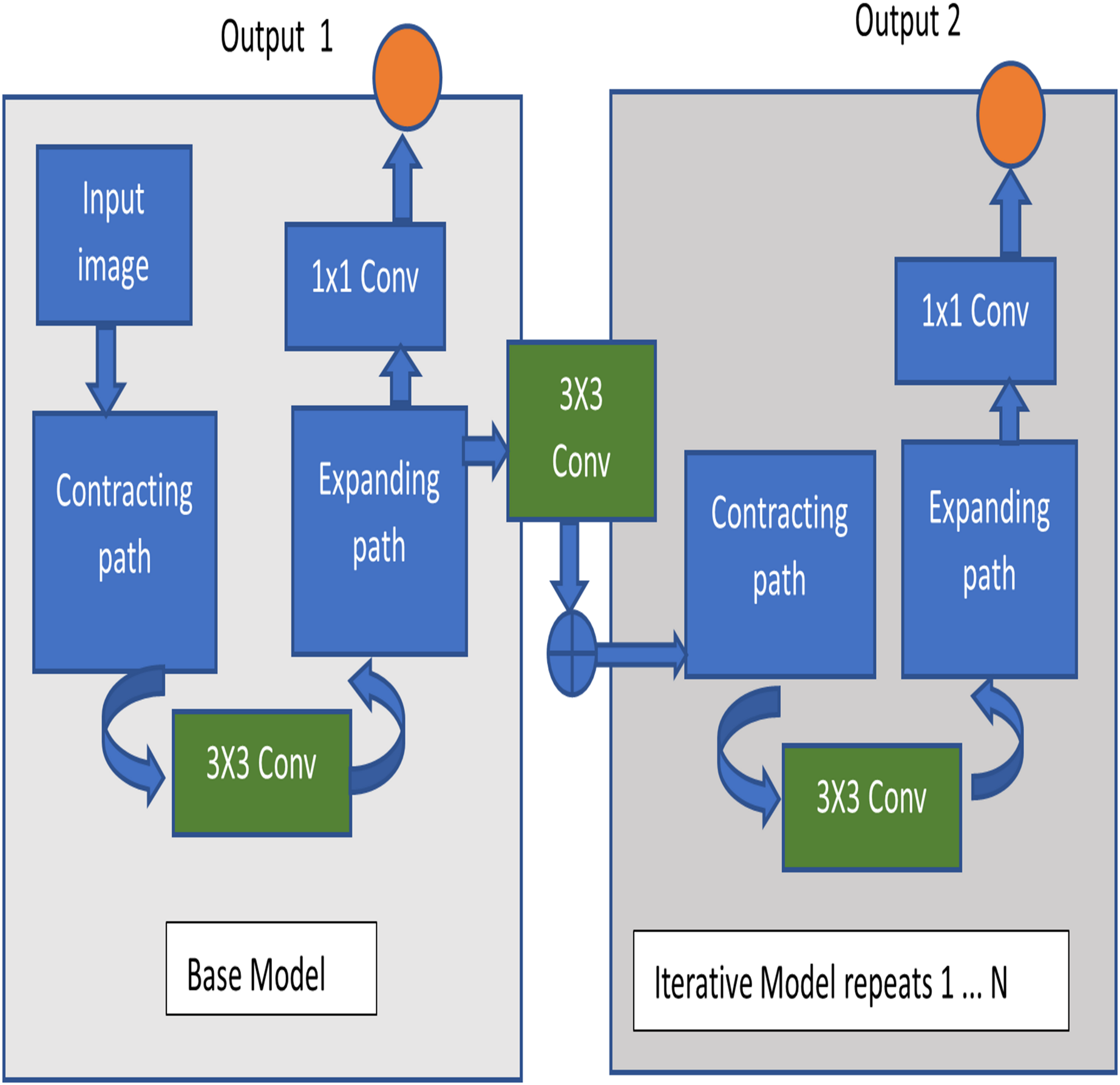
Proposed iterative UNet architecture
The architecture used in this image segmentation model is Iterative U-Net architecture. The fundamental structure of U-Net consists of a contracting and expanding path, giving it a U-shaped configuration and earning it the name U-Net. This architecture is primarily constructed as an end-to-end fully convolutional network (Sivagami et al., 2020). Illustrated in Fig. 5 is the diagram of the Iterative UNet architecture, depicting the iterative application of the U-Net structure in both encoding and decoding. This iterative process results in a U-shaped pattern and provides a comprehensive view of the convolutional and pooling layers involved. The UNet structure is applied iteratively for N-1 iterations, where an increase in N leads to a proportional increase in trainable parameters. This introduces a tradeoff between time, space complexity, and performance.
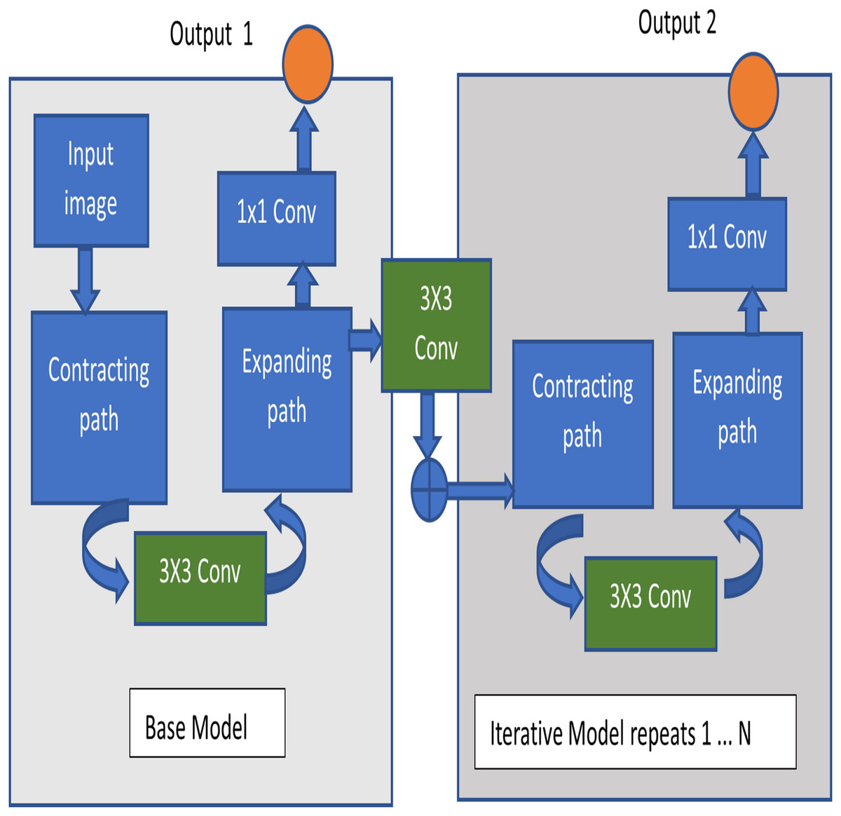
Figure 5: Iterative U-Net architecture.
The encoder part of the iterative UNet architecture consists of downsampling blocks, similar to the traditional UNet. Each downsampling block typically includes convolutional layers followed by pooling or strided convolutions to progressively reduce the spatial resolution while increasing the number of feature channels. This helps in capturing context and extracting high-level features. The output of each convolutional layer is given by Eq. (1),
(1) where Zl is the output, Wl is the weight matrix, Al−1 is the input from the previous layer, bl is the bias term, and σ is the activation function.
Instead of a single decoder, the iterative UNet incorporates multiple decoder blocks, each refining the segmentation results iteratively. Each decoder block takes the output of the previous decoder block and features from the corresponding encoder block. The output of each upsampling layer is given by Eq. (2),
(2) where Ul is the upsampled output. Concatenation of the upsampled output with the corresponding feature map from the encoder will be denoted in Eq. (3) as,
(3)
Skip connections are formed by concatenating feature maps from the encoder to the decoder to preserve spatial information. The final layer typically involves a 1 × 1 convolution to produce the segmentation output.
(4) where Y is the final output which is shown in Eq. (4). This iterative process helps in refining the segmentation progressively, allowing the model to capture more fine-grained details and improve accuracy.
Proposed UNet architecture with atrous spacial pyramid pooling module
The UNet architecture has been augmented with the ASPP module from the DeepLab V3+ variant. This integration involves placing the ASPP module before the decoder, facilitating the capture of multi-scale contextual information. The ASPP module comprises parallel atrous/dilated convolutions with distinct dilation rates, strategically employed to grasp context at varying resolutions. The resultant feature maps from these parallel convolutions are subsequently merged to form a more comprehensive representation of the input. By incorporating the ASPP module, the architecture effectively captures both local and global contextual information, thereby enhancing segmentation performance.
Expressing the U-Net architecture with ASPP mathematically involves a series of equations. For clarity, a conceptual representation of the U-Net with ASPP is presented here. It is important to note that this representation offers a high-level overview, and actual implementations may entail additional details and considerations. Let X denote the input image and Y represent the output segmentation mask. The U-Net with ASPP can be dissected into encoding and decoding stages, with the ASPP module typically integrated into the encoding stage to ensure the capture of multi-scale contextual information.
Encoding stage: U-Net involves down-sampling and capturing features at different scales. Input Convolution can be denoted as in Eq. (5),
(5) where Conv represents the convolution operation, W1 is the weight matrix, and b1 is the bias term. Down sampling can be denoted as in Eq. (6),
(6) where MaxPool is the max pooling operation.
ASPP module: can be denoted as Eqs. (7) and (8),
(7)
(8) where Convdilated is the dilated convolution operation, Wasppi represents the weights for each dilated convolution, and Concat denotes the concatenation operation.
Decoding stage:
The decoding stage involves up-sampling and combining features from the encoding stage. Upsampling will be denoted as in Eq. (9),
(9) where UpSample is the up-sampling operation. Skip connections will be denoted as in Eq. (10),
(10)
This step combines features from the up-sampled output and the corresponding feature map from the encoding stage. The decoder convolution will be denoted as in Eq. (11),
(11)
The output convolution is shown in Eq. (12),
(12)
Skip connections, similar to the UNet architecture, are used to bridge the encoder and decoder blocks. These connections help in preserving spatial information and gradients during the upsampling process, aiding in accurate localization of objects and maintaining fine details. Table 2 gives the model summary of the above implemented model with various dilation rates such as 2, 4 and 6.
| Layer (type) | Output shape | Param # |
|---|---|---|
| input_4 (InputLayer) | [(None, 256, 256, 3)] | 0 |
| conv2d_1(Conv2D) | (None, 256, 256, 64) | 1,792 |
| conv2d_2 (Conv2D) | (None, 256, 256, 64) | 36,928 |
| max_pooling2d_1 (MaxPooling2D) | (None, 128, 128, 64) | 0 |
| conv2d_3 (Conv2D) | (None, 128, 128, 128) | 73,856 |
| conv2d_4(Conv2D) | (None, 128, 128, 128) | 147,584 |
| max_pooling2d_2 (MaxPooling2D) | (None, 64, 64, 128) | 0 |
| conv2d_5(Conv2D) | (None, 64, 64, 256) | 295,168 |
| conv2d_6(Conv2D) | (None, 64, 64, 256) | 590,080 |
| conv2d_7(Conv2D) | (None, 64, 64, 256) | 590,080 |
| conv2d_transpose_1 (Conv2DTranpose) | (None, 128, 128, 128) | 131,200 |
| concatenate_1 (Concatenate) | (None, 128, 128, 256) | 0 |
| conv2d_8 (Conv2D) | (None, 128, 128, 128) | 295,040 |
| conv2d_9 (Conv2D) | (None, 128, 128, 128) | 147,584 |
| conv2d_transpose_2 (Conv2DTraspose) | (None, 256, 256, 64) | 32,832 |
| concatenate_2 (Concatenate) | (None, 256, 256, 128) | 0 |
| conv2d_10 (Conv2D) | (None, 256, 256, 64) | 73,792 |
| conv2d_11 (Conv2D) | (None, 256, 256, 64) | 36,928 |
| conv2d_12 (Conv2D) | (None, 256, 256, 10) | 650 |
| Total params: 2,453,514 Trainable params: 2,453,514 Non-trainable params: 0 |
||
Proposed pre-trained models for feature extraction
Proposed customized model
The convolution layer which extracts features by input image while preserving the relationship between image pixels. In this layer edge detection, blur, sharpen filters can be applicable to the input image. At each area on the input, matrix multiplication is performed by consolidating the outcome. The resultant feature map is explained as:
(13)
(14)
Equations (13) and (14) is the last layer’s output feature map’s width and height, where (Pa, Pb) is the dimension and height of the output feature map of the final layer and (Qa, Qb) is the kernel size, (Ta, Tb) that characterizes the total pixels kept away by the kernel in the r index and both the horizontal and vertical axes demonstrates the layer i.e., r = 1. Convolution operation is characterized as:
(15)
In Eq. (15), A1 (c, d) is a coplanar output feature map acquired by convolving the two-dimensional kernel R of size (Qa, Qb) and input feature map I. The sign * is utilized to address the convolution between I and J. The convolution operation is indicated as,
(16)
In Eq. (16), A1 (c, d) is a final convolution operation of feature map where there is a convolution between the I and J. When the image is huge, pooling layers are frequently used to reduce the number of parameters. To minimise the image’s dimensions, it either downsamples or upsamples. There are three different types of pooling: maximum, average, and sum. Max Pooling is mainly used to select the largest element from a feature map. Table 3 shows the layers created in customized model. Average pooling and dropout are used at appropriate places to reduce the number of parameters.
| Layer (type) | Output shape | Param # |
|---|---|---|
| conv2d_10 (Conv2D) | (None, 222, 222, 32) | 896 |
| average_pooling2d_2 | Average (None, 111, 111, 32) | 0 |
| batch_normalization_5 | Batch (None, 111, 111, 32) | 128 |
| conv2d_11 (Conv2D) | (None, 109, 109, 64) | 18,496 |
| conv2d_12 (Conv2D) | (None, 107, 107, 64) | 36,928 |
| average_pooling2d_3 | (Average (None, 53, 53, 64)) | 0 |
| batch_normalization_6 | (Batch (None, 53, 53, 64)) | 256 |
| conv2d_13 (Conv2D) | (None, 51, 51, 128) | 73,856 |
| conv2d_14 (Conv2D) | (None, 49, 49, 128) | 147,584 |
| conv2d_15 (Conv2D) | (None, 47, 47, 128) | 147,584 |
| max_pooling2d_2 | (MaxPooling2 (None, 24, 24, 128)) | 0 |
| batch_normalization_7 | (Batch (None, 24, 24, 128)) | 512 |
| conv2d_16 (Conv2D) | (None, 22, 22, 256) | 295,168 |
| conv2d_17 (Conv2D) | (None, 20, 20, 256) | 590,080 |
| conv2d_18 (Conv2D) | (None, 18, 18, 256) | 590,080 |
| conv2d_19 (Conv2D) | (None, 16, 16, 256) | 590,080 |
| max_pooling2d_3 | (MaxPooling2 (None, 8, 8, 256)) | 0 |
| batch_normalization_8 | (Batch (None, 8, 8, 256)) | 1,024 |
| flatten_4 (Flatten) | (None, 16384) | 0 |
| dense_15 (Dense) | (None, 64) | 1,048,640 |
| batch_normalization_9 | (Batch (None, 64) | 256 |
| dropout_13 (Dropout) | (None, 64) | 0 |
| dense_16 (Dense) | (None, 10) | 650 |
| Total params: 3,542,218 Trainable params: 3,541,130 Non-trainable params: 1,088 |
||
Pooling layers are commonly utilized to minimize the number of parameters when the image is large. It either uses upsampling or downsampling to reduce dimensionalities of the image. Then batch normalization (Khamparia et al., 2020) is used to make the data flow between intermediate layers of the neural network by making use of a higher learning rate.
Proposed hybrid model
The customized architecture is fused with the AlexNet architecture as well as with the ResNet architecture and EfficientNet B7. In the working model of the hybrid model, after being resized fed into UNet for segmentation and the segmented images are passed through the concatenated CNN model. Here the output layer of the first model is given as input to the second model thus concatenating two models to form hybrid architecture. The model hybridization is taken into account in the view of increasing the accuracy. After passing through the hybridized model, the images are classified.
Hyper parameter tuning
Hyper parameter tuning is utilized for expanding the productivity of the model. It does its little job to work on the accuracy of a model. The modification process holds significant importance, as certain alterations impact factors such as training computation time, convergence speed, and the utilization of processing units. Iterative hyperparameter tuning was consistently performed to enhance the precision of the proposed model and improve overall accuracy. Table 4 represents the parameters for the proposed models. For the experiment, the training is done for each CNN architecture along with the hyper parameter tuning. In time of training, the tuning of the parameters is done for the reducing the dimensionality of features, regularization for improvement capacities on the result layer respectively. During network training, a batch size of 128 was used for training and five for validation, balancing computational efficiency with generalization capacity. A learning rate of 0.001 was empirically chosen after tuning across multiple values (0.01, 0.005, 0.0005, 0.0001). A higher learning rate led to unstable convergence, while a lower rate slowed down training without performance gains. The chosen learning rate ensured stable convergence within 50 epochs, as shown by the training/validation accuracy and loss trends in Figs. 9 and 10, which display consistent improvements with minimal overfitting. Among the optimizers tested (Adam, AdaMax, AdaGrad, RMSprop), Adam provided the best tradeoff between convergence speed and accuracy, due to its adaptive moment estimation that efficiently handled sparse gradients. This choice resulted in faster convergence and reduced training loss, especially for deeper architectures such as the customized model concatenated with EfficientNetB7. The number of epochs was fixed at 50, as further extension showed saturation in accuracy improvements with minor fluctuations. The plotted learning curves also validate this convergence behavior.
| Parameter | Value |
|---|---|
| Batch size (Training data) | 128 |
| Batch size (Validation data) | 5 |
| Epoch | 50 |
| Optimizer | ADAM |
| Learning rate | 0.001 |
Performance metrics
In order to evaluate the efficacy of the proposed classification and segmentation technique, six frequently used assessment metrics—namely accuracy, sensitivity, specificity, precision, and recall—are employed. The terms true positive (TP), true negative (TN), false positive (FP), and false negative (FN) are designated accordingly. Accuracy is defined as:
(17)
The proportion of true positive result to real positive is called the sensitivity in detecting disease and it is calculated as follows:
(18)
The proportion of negative results to all real negatives is called specificity or true negative rate (TNR). If the specificity is high, it indicates that the model is good in identifying the healthy leaves.
(19)
The ratio of positive inspections that are anticipated accurately to the total positively anticipated inspections is called precision.
(20)
The ratio of positive inspections that are anticipated accurately to all the inspections in actual class is called recall.
(21)
The IoU or Jaccard Index is a metric used to evaluate the accuracy of segmentation. In this context, TP denotes the count of pixels accurately classified as foreground (correctly segmented), FP indicates the count of pixels erroneously classified as foreground (over-segmented), and FN denotes the count of pixels inaccurately classified as background (under-segmented).
(22)
Results
The first experiment is to compare the results of the non-segmented images with the ResNet50, AlexNet, EfficientNet B0, EfficientNet B7, customized and Hybrid models. These architectures are trained with plant village dataset and tested by test data images of the same. It is also compared by changing weights of these models. The results of the experiments are presented in Table 5, revealing that the tailored model incorporating EfficientNet achieves superior accuracy and lower loss. Notably, the customized model not only demonstrates enhanced accuracy but also exhibits a notably reduced time requirement for each step.
| Deep learning architectures | Parameters (in Millions) |
Training time (in hours) |
Training accuracy |
Validation accuracy |
|---|---|---|---|---|
| ResNet-50 | 23.5 M | 15.2 | 97.0 | 93.5 |
| AlexNet | 58.3 M | 25.3 | 92.9 | 91.2 |
| EfficientNet B0 | 5.3 M | 7.5 | 93.9 | 92.9 |
| EfficientNet B7 | 66.2 M | 28.6 | 98.0 | 95.8 |
| Customised Model | 3.54 M | 3.3 | 98.2 | 96.9 |
| HybridResNet-50 with Customised Model | 85.4 M | 35.5 | 94.1 | 91.6 |
| Hybrid AlexNet with Customised Model | 100.7 M | 10.5 | 93.5 | 93.3 |
| Hybrid EfficientNet B7 with Customised Model | 72.3 M | 30.3 | 98.9 | 98.5 |
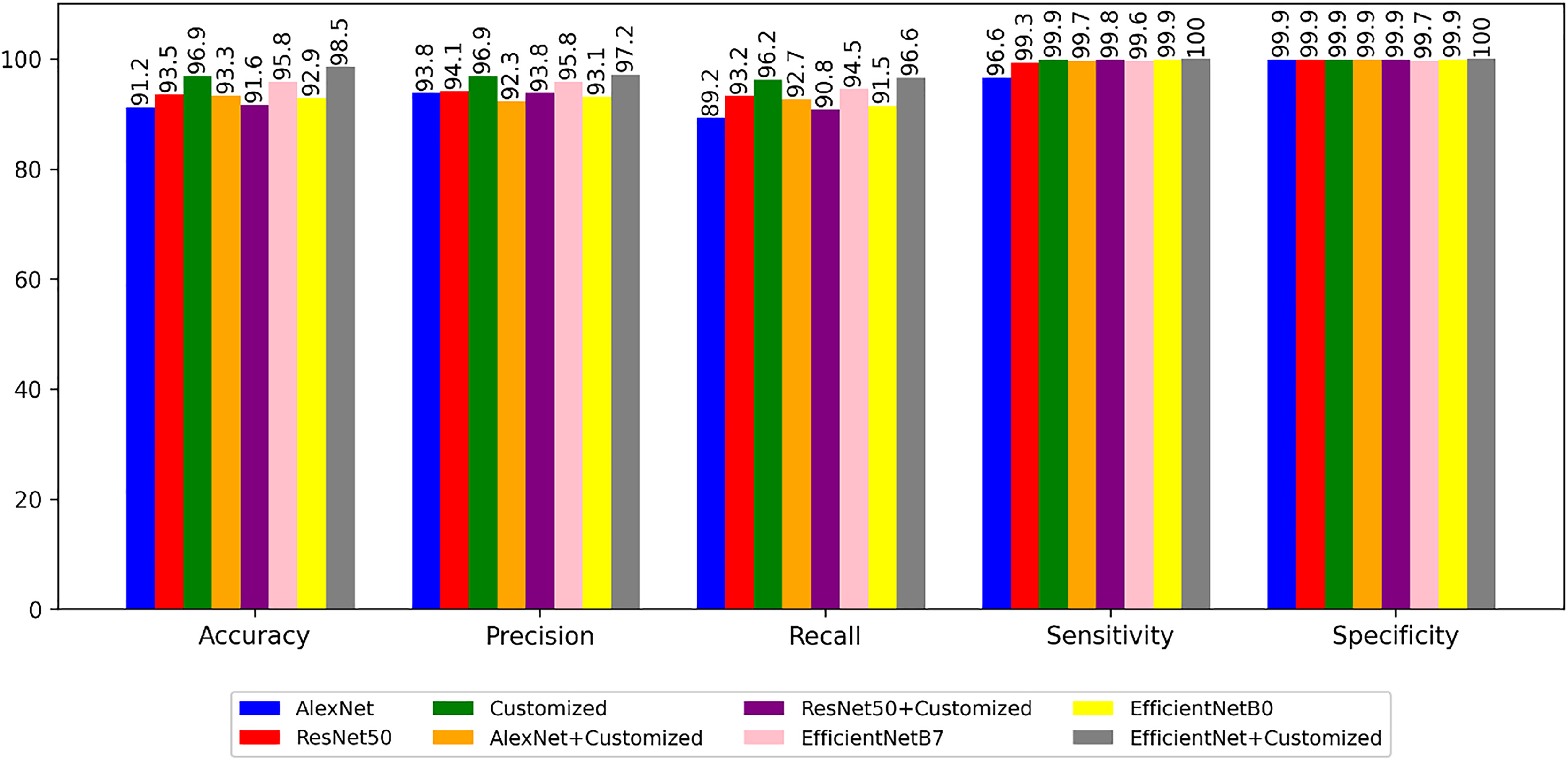
Figure 6 illustrates a performance metrics comparison, encompassing accuracy, precision, recall, sensitivity, and specificity, between the predefined and customized architectures. The next experiment is to segment the images using segmentation architectures like UNet, DeeplabV3+, iterative UNet and UNet with ASPP module.
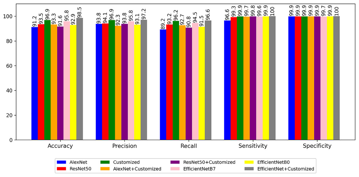
Figure 6: Performance of the models with non-segmented images.
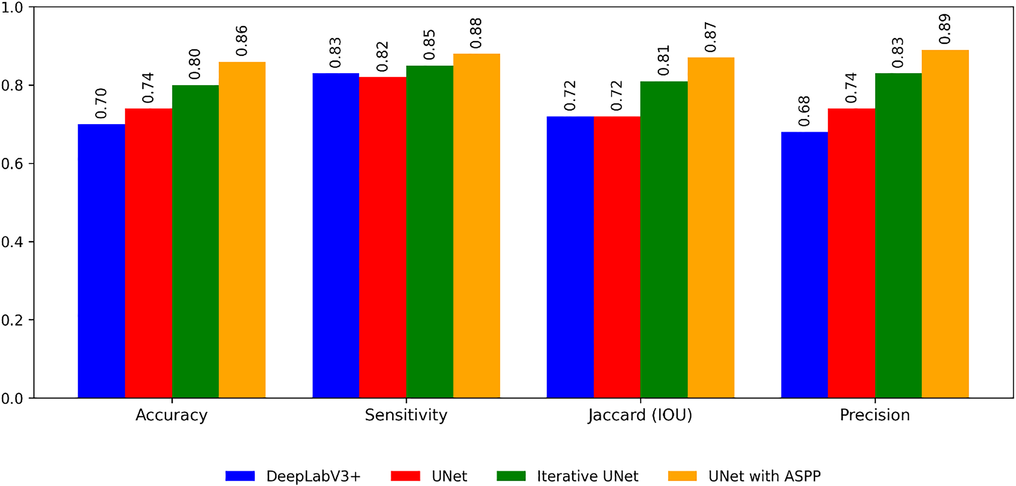
The following Table 5 shows the segmentation performance of each model for the plant village dataset.
From the Table 6 and Fig. 7 it is inferred that, U-Net tends to perform well in terms of accuracy because of its encoder-decoder structure with skip connections. The skip connections allow for the fusion of both low-level and high-level features, enabling the model to capture detailed spatial information during segmentation. As a result, U-Net can effectively delineate object boundaries and generate accurate pixel-level predictions.
| Metrics | DeepLabV3+ | UNet | Iterative UNet | UNet with ASPP |
|---|---|---|---|---|
| Accuracy | 0.70 | 0.74 | 0.90 | 0.86 |
| Sensitivity | 0.83 | 0.82 | 0.86 | 0.88 |
| Jaccard (IOU) | 0.89 | 0.72 | 0.87 | 0.92 |
| Precision | 0.74 | 0.68 | 0.80 | 0.89 |
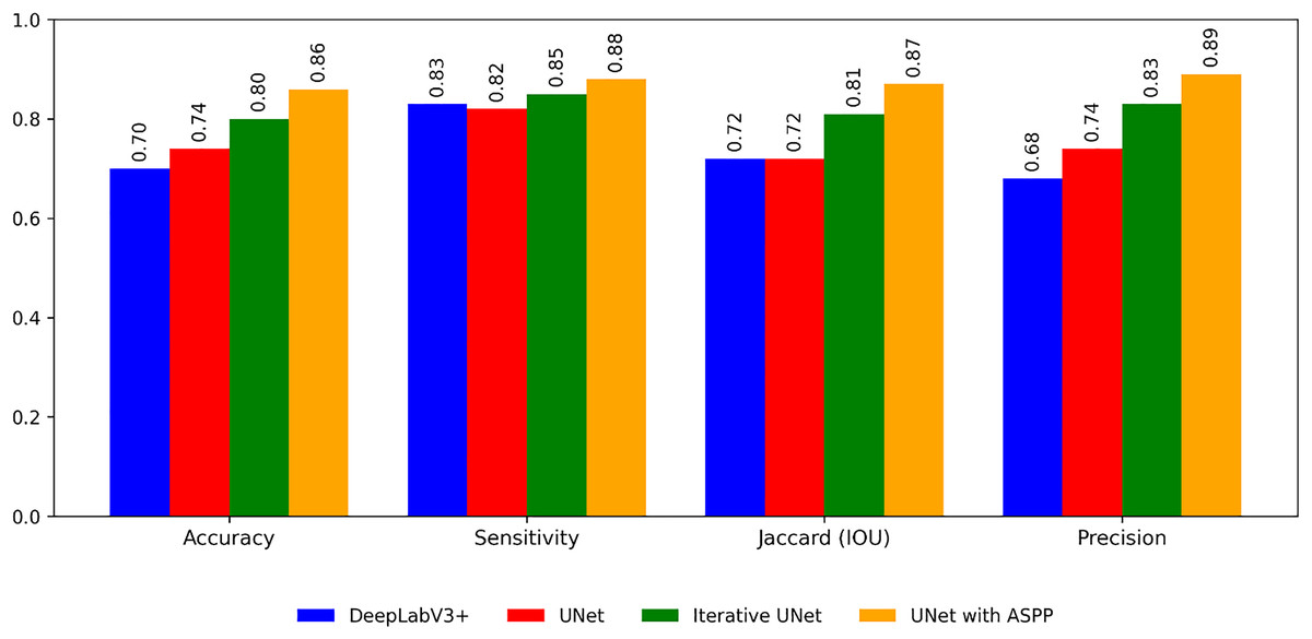
Figure 7: Performance of the segmentation algorithms.
Whereas DeepLabv3, on the other hand, focuses on capturing multi-scale contextual information through the use of dilated convolutions and ASPP. By incorporating dilated convolutions, DeepLabv3 can aggregate information from a wider receptive field, which helps in understanding global context and handling objects of varying scales. ASPP further enhances this capability by performing convolutions at multiple dilation rates. The Jaccard IOU metric, which measures the overlap between predicted and ground truth segmentation masks, evaluates the model’s ability to capture object shapes and contours accurately.
So the proposed segmentation models iterative UNet and UNet with ASPP outperforms the above traditional models in the following ways. Iterative U-Net aims to enhance accuracy, Jaccard IOU, precision, and sensitivity through an iterative feedback loop that refines the segmentation predictions. By iteratively updating the predictions based on the input image and previous iterations, iterative U-Net aims to improve segmentation performance in terms of these evaluation metrics. Whereas in the other model UNet with ASPP module, ASPP is incorporated to UNet architecture similar to DeepLabV3+. So it helps to capture multi-scale contextual information. By considering different dilation rates in the ASPP module, the model can effectively analyze the image at multiple scales and gather contextual cues. This enables the proposed model to have a more comprehensive understanding of the scene, distinguishing true object boundaries from background clutter and reducing the likelihood of false positive predictions.
The third experiment is to compare the results of the segmented images using UNet with ASPP with the classification models discussed. The inference obtained from Table 7 is that Hybrid EfficientNet B7 with customized Model gave a better accuracy when comparing to other models. But the tradeoff between time and accuracy shows that customized model is producing a nearby accuracy as like hybrid models as well as with reduced time complexity.
| Deep learning architectures | Parameters (in Millions) |
Training time (in hours) |
Training accuracy | Validation accuracy |
|---|---|---|---|---|
| ResNet-50 | 23.5 M | 11.2 | 94.79 | 95.5 |
| AlexNet | 58.3 M | 15.3 | 93.31 | 92.8 |
| EfficientNet B0 | 5.3 M | 4.5 | 94.1 | 93.1 |
| EfficientNet B7 | 66.2 M | 16.3 | 98.7 | 96.8 |
| Customised Model | 3.54 M | 2.6 | 98.9 | 97.5 |
| ResNet-50 with Customised Model | 85.4 M | 26.4 | 97.8 | 97.4 |
| Hybrid AlexNet with Customised Model | 100.7 M | 8.6 | 94.64 | 94.6 |
| Hybrid EfficientNet B7 with Customised Model | 72.3 M | 18.3 | 99.6 | 99.7 |
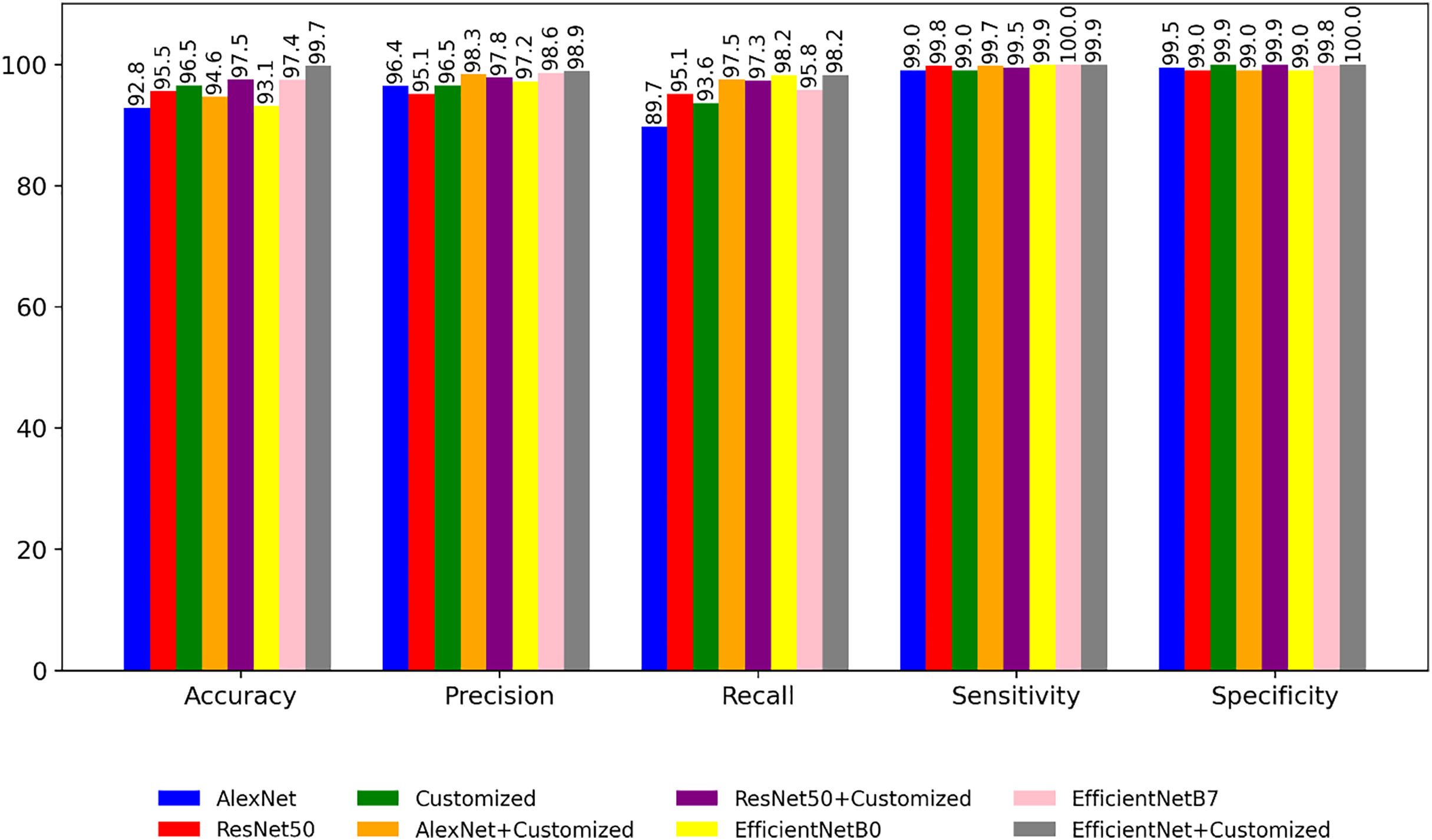
Figure 8 is a bar graph representation that shows the comparison of performance of the pre-trained models for the segmented images based on performance metrics like accuracy, precision, recall etc. Comparing with Fig. 6, it is evident that the classification accuracy shows a consistent increase while the time complexity decreases when performing classification after image segmentation. In the fourth experiment, the application of different optimizers are explored on the customized model. The result shown in Tables 8 and 9 indicates that a customized model with Adam optimizer has higher accuracy as well as lower loss.
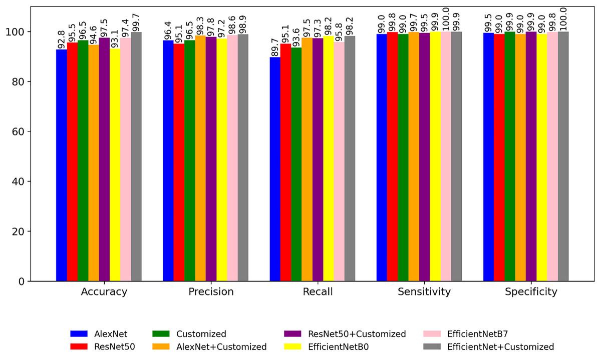
Figure 8: Performance of the models with segmented images.
| Optimisers | Training accuracy |
Validation accuracy | Precision | Recall | Specificity | Sensitivity |
|---|---|---|---|---|---|---|
| Adam | 99 | 98.8 | 97.9 | 97.6 | 100 | 99.8 |
| Adamax | 98 | 96.4 | 97.5 | 97 | 100 | 100 |
| Adagrad | 96.96 | 96.07 | 97.76 | 96.74 | 100 | 100 |
| RMSprop | 96.85 | 91.36 | 92.97 | 90.56 | 99.66 | 99.66 |
| Optimisers | Training accuracy |
Validation accuracy | Precision | Recall | Specificity | Sensitivity |
|---|---|---|---|---|---|---|
| Adam | 99.9 | 99.8 | 98.3 | 98.1 | 100 | 100 |
| Adamax | 98.04 | 98.04 | 98.25 | 97.81 | 100 | 99.97 |
| Adagrad | 95.94 | 96.74 | 97.41 | 96.01 | 100 | 100 |
| RMSprop | 95.22 | 91.56 | 93.16 | 89.63 | 99.73 | 99.9 |
In the final testing phase, 20 images were utilized to represent 10 distinct classes. Throughout this testing process, the models put forth exhibited an impressive testing accuracy of 97%. It is noteworthy that the ResNet50 model emerged with the highest success rate, accompanied by lower losses and convergence times in comparison to models employing alternative pre-trained networks.
The results are obtained for the crop leaf diseases of corn, tomato and potato from the PlantVillage dataset. The first experiment is designed to analyze the outcomes of the non-segmented images with the CNN models and hybrid models. The second experiment is to compare the results of segmented images with the CNN models and the hybrid model.
Performance of architectures with and without segmentation
Graphical representation of customized model
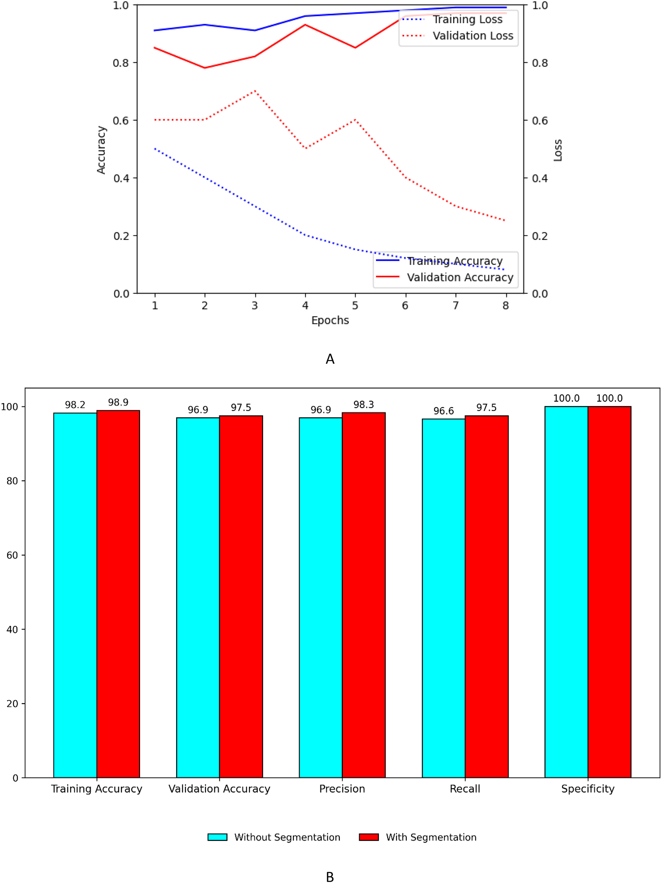
Figure 9A shows the training and validation, accuracy and loss curves of customized model. Figure 9B shows the performance improvement of the customized model with segmentation using UNet with ASPP architecture.
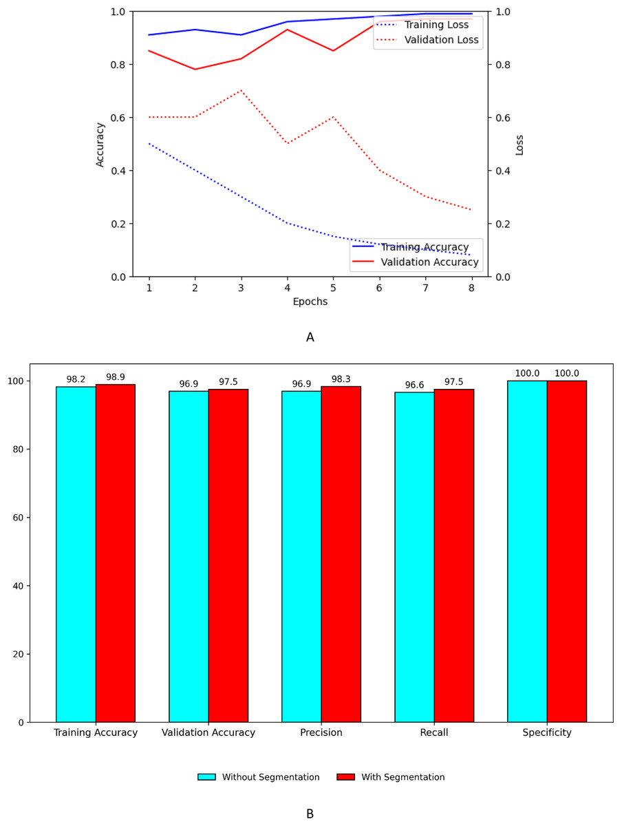
Figure 9: Performance plots of customized model (A) accuracy and loss with segmentation (B) comparison with and without segmentation.
Graphical representation of customized model+EfficientNet B7
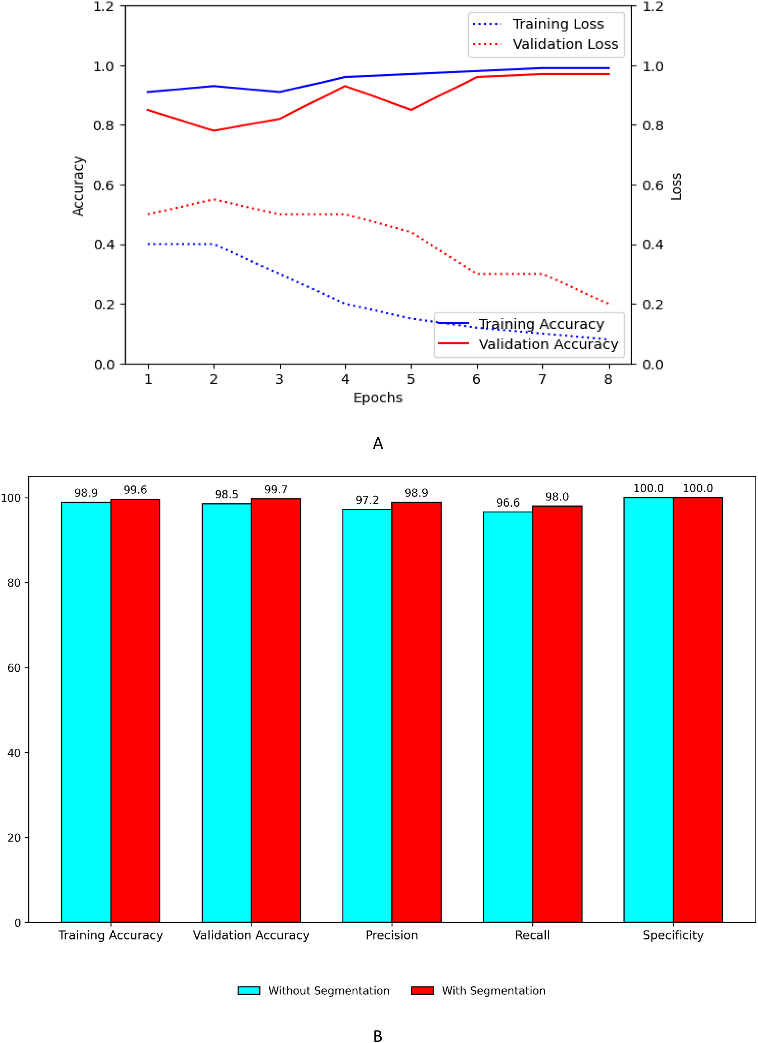
Figure 10A shows the training and validation, accuracy and loss curves of customized model when concatenated with EfficientNet B7. Figure 10B shows the performance improvement of the concatenated customized model with segmentation using UNet with ASPP architecture.
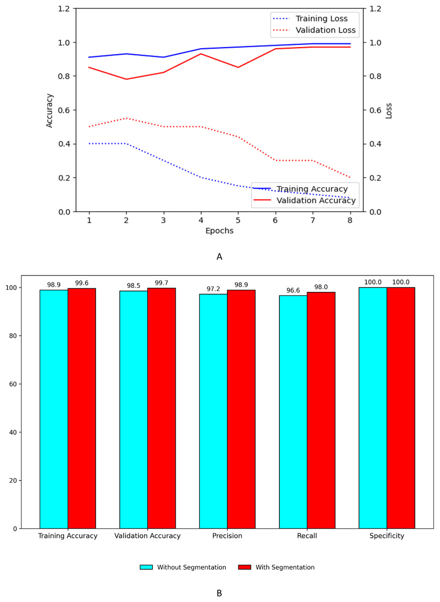
Figure 10: Performance plots of customized model with EfficientNet B7 (A) accuracy and loss with segmentation (B) comparison with and without segmentation.
Discussion
Table 10 shows the validation accuracy attained by pre-trained, customized and hybrid models by using segmented and non-segmented images.
| Methods | Dataset | Accuracy | ||
|---|---|---|---|---|
| Model name | With segmentation | Without segmentation | ||
| Segmentation, feature extraction |
Plant village (corn, potato and tomato leaves) | ResNet-50 | 95.5 | 93.5 |
| AlexNet | 92.8 | 91.2 | ||
| EfficientNet B0 | 93.1 | 92.9 | ||
| EfficientNet B7 | 96.8 | 95.8 | ||
| Customised Model | 99.8 | 96.9 | ||
| ResNet-50 with Customised Model | 97.4 | 91.6 | ||
| Hybrid AlexNet with Customised Model | 94.6 | 93.3 | ||
| Hybrid EfficientNet B7 with Customised Model | 99.7 | 98.5 | ||
Table 11 plays a pivotal role in encapsulating the essential references for the proposed work, meticulously outlining the various models, methodologies, and datasets that were leveraged in the referenced studies. This comprehensive compilation serves as a rich repository of insights, offering a nuanced perspective on the underpinnings of the research.
| S.No | Author | Reference no | Methods | Models and algorithm | Dataset | Accuracy (%) |
|---|---|---|---|---|---|---|
| 1 | KhaoulaBelhajSoulami | Soulami et al. (2021) | Segmentation | UNet | DDSM, Inbreast | 90.5 |
| 2 | YonghuaXiong | Xiong et al. (2020) | Segmentation | AISA based on GrabcutAlgorithm, MobileNet | PlantVillage + expanded dataset | 80 |
| 3 | Muhammad Attique Khan | Khan et al. (2018) | Coefficient based segmentation, feature fusion | VGG16, caffeAlexnet, multi class SVM | PlantVillage, CASC-IFW | 98.60 |
| 4 | T. Daniya | Daniya & Vigneshwari (2021) | Segmentation | SegNet, Deep RNN, RSW algorithm | Rice detection dataset | 90.5 |
| 5 | Shuo Chen | Chen et al. (2021) | Segmentation | BLS model based on UNet | Own dataset | 98.2 |
| 6 | Md. Arifur Rahman | Rahman et al. (2019) | Segmentation | RGB threshold | PlantVillage | 99.25 |
| 7 | YahyaAltunta | Altuntaş & Kocamaz (2021) | Feature extraction, concatenation | AlexNet, GoogLeNet and ResNet-50 | PlantVillage | 96.99 |
| 8 | Faye Mohameth | Mohameth, Bingcai & Sada (2020) | Feature extraction | ResNet 50, Google Net, VGG-16 | PlantVillage | 99.53 |
| 9 | Vinod Kumar | Kumar et al. (2020) | Feature extraction | ResNet34 | Open image dataset | 99.40 |
| 10 | Malliga Subramanian | Subramanian, Shanmugavadivel & Nandhini (2022) | Transfer learning and hyper- parameters optimization | VGG16, ResNet50, InceptionV3, and Xception | PlantVillage | 93 |
| 11 | Mobeen-ur-Rehman | Mobeen-ur-Rehman et al. (2019) | Feature extraction | Customised CNN model | MESSIDOR | 98.94 |
| 12 | ShradhaVerma | Verma, Chug & Singh (2020) | Transfer learning and feature extraction | AlexNet, SqueezeNet and Inception V3 | PlantVillage | 93.4 |
| 13 | Chunshan Wang | Wang et al. (2021) | Segmentation, | DeepLabV3 ,UNet | Self collected dataset | 92.85 |
| 14 | Bandar Alotaibi | Alotaibi & Alotaibi (2020) | Hybrid approach | hybrid deep ResNet-Inception | Pavia University, Pavia Centre scenes, Salinast and Indian Pines datasets |
99.02 |
| 15 | Yangyang Li | Li et al. (2019) | Deep feature fusion | Deep ResNet50 and VGG16 | UCM, NWPURESISC45 |
94.03 |
| 16 | Mohana Saranya | Proposed work | Hybrid approach, segmentation, classification | Customised model | PlantVillage (corn, potato and tomato leaves) | 99.8 |
| Hybrid EfficientNet B7 with customised model | 99.7 |
Upon a closer examination of the comparative results delineated in Table 11, a discernible trend emerges. It becomes evident that the amalgamation of a customized architecture with the incorporation of pretrained models, such as the notable EfficientNet B7, alongside an adept segmentation process, yielded superior accuracy outcomes when contrasted with the standalone pretrained models. This nuanced observation underscores the efficacy of the proposed approach, highlighting the synergistic impact of a tailored architecture in conjunction with state-of-the-art pretrained models. The meticulous fusion of these components not only enhances accuracy but also signifies a noteworthy stride towards optimizing model performance, thus validating the strategic choices made in the course of this research endeavour.
Conclusions
In this study, both the proposed customized model and its combination with the pretrained EfficientNet B7 architecture have yielded highly promising results in the realm of classification. Notably, the application of segmentation to the input dataset, utilizing the UNet with ASPP approach before feeding it into the classification model, further elevated accuracy levels. The proposed methodology has demonstrated superior performance compared to existing approaches, exhibiting higher accuracy and enhanced overall efficiency. The incorporation of segmentation techniques played a pivotal role in boosting accuracy when compared to non-segmented approaches. Additionally, the concatenated model, which fuses the strengths of individual models, showcased superior performance, emphasizing the synergistic benefits of combining segmentation and classification processes. Thus, the proposed approach emerges as a robust and effective solution, excelling in both performance and accuracy metrics.
The utilization of the plant village dataset for model training and evaluation underscores the real-world applicability of the approach in the context of diverse plant diseases across multiple species. Looking ahead, future research endeavors could explore extending this approach to datasets featuring an increased number of classes and diverse compositions. Additionally, investigating methods to optimize computational speed could further enhance the practicality and scalability of the proposed methodology. In summary, the study not only establishes the effectiveness of the proposed customized models and segmentation techniques but also positions them as advanced solutions that outperform existing approaches in the critical task of plant disease classification. As agriculture and technology continue to intersect, the findings contribute to the evolving landscape of precision agriculture, offering a potent framework for accurate and efficient disease identification and classification in diverse plant species.
Limitation
While the proposed methodology achieved high accuracy, it relies on the PlantVillage dataset, which was collected under controlled conditions. This may limit its performance in real-world scenarios where lighting, background clutter, occlusions, and noise vary significantly. Real-world agricultural images often contain challenges not present in the dataset. To improve generalization, future work should include field-collected datasets and use techniques like data augmentation (e.g., lighting jitter, occlusion simulation) and domain adaptation (e.g., transfer learning with field images). The approach also involves high computational costs due to segmentation and deep classification models. This may limit deployment on resource-constrained devices. Optimization for faster, lightweight models is a future need. Lastly, the study focused on a relatively constrained number of classes and disease types, suggesting the need for future research to expand the methodology’s applicability to datasets with greater class diversity and composition. Addressing these limitations is essential for ensuring the robustness and adaptability of the approach in broader agricultural contexts.