
A robust deep learning model for fall action detection using healthcare wearable sensors
- Published
- Accepted
- Received
- Academic Editor
- Consolato Sergi
- Subject Areas
- Artificial Intelligence, Computer Vision, Data Mining and Machine Learning, Neural Networks
- Keywords
- Machine learning, Data mining, Artificial intelligence, Deep learning, Human detection, Patterns recognition, Healthcare monitoring
- Copyright
- © 2025 Alazeb et al.
- Licence
- This is an open access article distributed under the terms of the Creative Commons Attribution License, which permits unrestricted use, distribution, reproduction and adaptation in any medium and for any purpose provided that it is properly attributed. For attribution, the original author(s), title, publication source (PeerJ Computer Science) and either DOI or URL of the article must be cited.
- Cite this article
- 2025. A robust deep learning model for fall action detection using healthcare wearable sensors. PeerJ Computer Science 11:e3300 https://doi.org/10.7717/peerj-cs.3300
Abstract
The proposed technique begins with Butterworth’s sixth-order filtering of the data followed by segmentation through Hamming window application. The identification of essential patterns is achieved through the utilization of feature extraction methods which include State Space Correlation Entropy (SSCE) coefficients together with Mel Frequency Cepstral Coefficients (MFCC), Linear Predictive Cepstral Coefficients (LPCC), Parseval’s energy and Auto-Regressive (AR) coefficients. The features are selected through Particle Swarm Optimization (PSO) optimization then Long Short-Term Memory (LSTM) networks execute the classification process. The method received experimental assessment using three publicly available datasets named UP-Fall, HealthLINK_Falls, and UR-Fall. The proposed method achieves a substantial improvement in classification results compared to traditional approaches while demonstrating enhanced accuracy outcomes in experiments. This methodology demonstrates exceptional performance for fall action detection systems because it combines advanced preprocessing techniques with robust feature extraction methods and LSTM networks optimized through PSO.
Introduction
Inertial sensors containing accelerometers and gyros achieved significant advancements because of micro-sensor and wireless communication technology improvements. Recent sensor technology enables manufacturers to create declining dimensions in their products without sacrificing performance meaning they are suitable for diverse portable devices like mobile phones and tablets and smartwatches. Consequently, wearable inertial sensors have been employed in a variety of applications, including human-machine interaction, user authentication, driving behavior analysis, fall detection for elderly care, rehabilitation and therapy, sports training, and daily activity monitoring (Yu, Qiu & Xiong, 2020). This has made action and fall detection systems using wearable sensors a prominent research area in fields such as healthcare, artificial intelligence (AI), and human-computer interaction.
This work investigates improvements in fall action detection with inertial sensory devices as its central research subject. The present difficulty with fall action detection systems continues because it is complex to segment action signals and training and testing sensors require proper alignment to work well together for similar action classes. The suggested research methodology develops a sophisticated system to detect both fall actions despite different obstacles. The processing system includes Butterworth sixth-order filter operations as pre-processing followed by Hamming window segmentation to split the data. The feature extraction process involves extracting key features such as State Space Correlation Entropy (SSCE), Mel Frequency Cepstral Coefficients (MFCC), Linear Predictive Cepstral Coefficients (LPCC), Parseval’s energy and Auto-Regressive (AR) coefficients. The process begins by applying Particle Swarm Optimization (PSO) to select features which are then classified through Long Short-Term Memory (LSTM) networks. The performance studies conducted on UP-Fall and UR-Fall systems concluded that the implemented detection system produces better results than standard detection methods during experimental testing. These research components are the main contributions of this study:
Data processing with Butterworth sixth-order filters and subsequent segmentation through Hamming windows enhances the extraction reliability of signals especially when sensor conditions vary.
The proposed framework uses a combination of SSCE coefficients together with MFCC, LPCC, Parseval’s energy, and AR coefficients as features for precise locomotion transition detection.
Feature selection based on the PSO system achieves optimization of discriminative features that are used for classification purposes.
LSTM networks form the basis for classification because they maintain superior capabilities to recognize sequential patterns related to complex actions and fall events.
The proposed system underwent thorough evaluation on the UP-Fall and UR-Fall datasets to prove its superior accuracy and reliability compared to standard techniques.
The implemented approach successfully handles sensor inconsistency problems alongside variation issues from both speed changes and movement styles and performs precise matching of equivalent action categories.
Related work
Recent researchers have utilized artificial intelligence to improve effective human routine analysis in health monitoring fields. According to the literature, this research primarily focuses on two key approaches.
Health routines via machine learning
Many researchers have extensively studied machine learning-based methods for improving health routines. Researchers from Arvindhan, Sharma & Kumar (2023) developed a sensor-powered machine learning system that examines human health activities using Accelerometer and Gyro to interpret body motions. Multiple tracking algorithms like Random Forest, K-Nearest Neighbor (KNN), Support Vector Machine (SVM), and Logistic Regression function within the system to analyze the walking sleeping, and running of users. The presented graphical results offer beneficial knowledge points for doctors and dietitians to develop practical health treatment strategies. Bar charts and pie charts in the user interface help people gain a better perception of their routines. Hoffmann, Steinhage & Lauterbach (2017) built a technical system using machine learning detection methods to monitor unsolicited health routine changes across extended time intervals. The system uses sensors with a unique capacitance detection system to track human behaviors including sleep behavior and walking methods. A processing scheme obtains behavioral information from sensor data for analysis through a learning algorithm. The algorithm finds irregular conduct in everyday practices to generate early detection alerts about health alterations while needing no input from patients. A healthcare bot developed by Shankhdhar et al. (2021) uses machine learning to detect patient symptoms which results in specific health routine suggestions. The system uses user input analysis to create personalized diet plans and workouts while matching patients with medical professionals. The system uses the Decision Tree algorithm to detect diseases from patient symptoms which improves diagnostic outcomes. The system develops patient interaction through Python libraries that generate a simulated communication environment to boost user activity and healthcare system management. Toapanta et al. (2005) examined whether machine learning techniques could enhance physical exercise outcome predictions for hypertensive patients. Naive Bayes along with Decision Tree and Logistic Regression participated in modeling the prescribed exercises’ effects according to their research. Analysis using the Decision Tree algorithm produced the most optimal results as it reached an accuracy rate of 79% from the data. The predictive model functions as a part of the Food Corporation of India (FCI) Research Project platform to help health practitioners design customized workout plans. Performance measures including accuracy precision and recall allow the system to measure model effectiveness toward enhancing health results for hypertensive people. Machine learning systems based on weak supervision methods served as the focus of research by Banovic et al. (2017) to create behavioral models that detect actions that affect well-being. They have designed their method to use weak labeling from demonstrated routines which minimizes the need for extensive manual data labeling. The system detects aggressive driving behavior through its identification process and then creates opportunities for patients to reflect on their actions while correcting their behavior. Through machine learning approaches researchers can develop practical observations which support health-promoting actions and general wellness enhancement.
Health routine via deep learning
Healthcare received major enhancements through deep learning methods for monitoring and management as these learning approaches generate exact outputs by using flexible process models. User movement observation and exercise statistics collection occurred in a web application built with React through webcam analysis powered by TensorFlow.js according to Salian & Naik (2023). Users achieve exact motion tracking for fitness judgment through webcam-based monitoring provided by the system. Activity monitoring systems utilizing Node.js technology and MongoDB storage systems achieve revolutionary capability due to their ability to provide real-time user experiences. Zargar, Zargar & Mehri (2023) demonstrated Deep Neural Network (DNN) research based on Convolutional Neural Networks (CNNs) and Recurrent Neural Networks (RNNs) to improve healthcare data prediction accuracy. The system provides medical image processing through Natural Language Processing (NLP) technology and then merges CNNs and RNNs to achieve top speed for clinical data interpretation. The multiple layers within deep learning systems help represent data better and improve generalization to achieve superior predictions for diverse clinical input information. Nisar et al. (2021) joined other researchers to conduct research focusing on deep learning techniques for healthcare applications in their investigation. Medical imaging with supervised CNNs and Deep CNNs segments brain structures during supervised operations but relies on Boltzmann machines and autoencoders to accomplish successful unstructured data processing in unsupervised stages. Healthcare professionals improve their diagnoses by employing these methods to build intelligent AI diagnostic tools that lower healthcare costs at the same time they develop disease identification algorithms. The article examines two key sections: the data management barriers posed by unstructured information first followed by proof of concept research into optimized unsupervised learning framework. The research team led by Kaul, Raju & Tripathy (2022) demonstrated how deep neural networks can be utilized for disease diagnosis and disease treatment methods for cancer, diabetes, and Alzheimer’s. These processing methods help researchers study disease development patterns and create unique treatment programs for patients as well as improve medical care. Deep learning functions through brain-like processing that leads to high efficiency when analyzing medical data thus it stands as a powerful instrument for monitoring complex medical diseases. The system by Fan (2019) creates a deep learning platform for health recommendations that gathers data from wearable devices before investigation. The data enters a deep learning network that generates personalized food and movement plan indexes through its processing. Data mining of large datasets allows the system to create customized recommendations that generate health management solutions from individual user data. Research by Ventrilho dos Santos & Carvalho (2016) demonstrated that clinical diagnosis accuracy highly depends on deep learning models especially when utilizing CNNs with back-propagation algorithms. Such models demonstrate superior effectiveness compared to traditional approaches as well as human interpretation in analyzing medical images and disease recognition tasks. Deep learning exemplifies its ability to enhance medical diagnosis precision through accurate clinical assessments and assists doctors with exact treatment plan generation according to individual patient information. The authors in Shekhar et al. (2024) developed deep learning models including CNN, CNN-LSTM, and Multi-Headed CNN-Bidirectional Long Short-Term Memory (BiLSTM) to recognize human activities through wearable sensors. According to their study which used the UCI Human Activity Recognition (HAR) dataset the Multi-Headed CNN-BiLSTM model achieved superior performance at all levels of accuracy and precision evaluation along with recall and F1-scores. Advanced deep learning architectures demonstrate their capabilities for healthcare smart applications by providing outstanding tracking of physical activities. The summary of advantages and limitations of existing approaches is displayed in Table 1.
| Study | Approach | Advantages | Limitations |
|---|---|---|---|
| Arvindhan, Sharma & Kumar (2023) | ML-based system with accelerometer & gyro using RF, KNN, SVM, LR | Simple setup; Multiple algorithms tested; Provides visual feedback for users | Limited to basic activities; May not generalize to varied environments |
| Hoffmann, Steinhage & Lauterbach (2017) | Capacitive sensor system + Machine Learning (ML) for long-term monitoring | Detects subtle behavioral changes; Low user intervention | Specific sensor hardware; Potentially high deployment cost |
| Shankhdhar et al. (2021) | Healthcare bot using decision tree | Personalized diet/workout plans; Integrates symptom-based diagnosis | Relies heavily on user input; Limited physical activity detection |
| Toapanta et al. (2005) | Naive Bayes, Decision tree, Logistic regression for exercise prediction | Supports personalized exercise plans; Achieves up to 79% accuracy. | Focused on hypertensive patients; Narrow activity scope. |
| Banovic et al. (2017) | Weak supervision-based behavioral modeling | Reduces manual labeling effort; Detects irregular driving behavior | Limited validation in healthcare; May miss rare patterns |
| Salian & Naik (2023) | Webcam-based activity tracking (TensorFlow.js) | No wearable needed; Real-time tracking | Requires stable camera setup; Limited to visible activities |
| Zargar, Zargar & Mehri (2023) | CNN + RNN for medical image and sensor fusion | High prediction accuracy; Works on multimodal data | High computational cost; Needs large labeled datasets |
| Nisar et al. (2021) | CNNs, Boltzmann machines, autoencoders | Handles structured & unstructured data; Useful for diagnosis | Complex architecture; Difficult to deploy on low-power devices |
| Kaul, Raju & Tripathy (2022) | DNNs for disease diagnosis (cancer, diabetes, Alzheimer’s) | Can learn complex patterns; Applicable to multiple diseases | Not activity-specific; Requires medical datasets |
| Fan (2019) | Wearable data + DL for personalized recommendations | Generates individual health plans; Data-driven | Privacy concerns; Dependent on device accuracy |
| Shekhar et al. (2024) | CNN, CNN-LSTM, Multi-Headed CNN-BiLSTM on UCI HAR | High accuracy and F1-scores; Robust sequential modeling | Requires high computation; Dataset-specific tuning |
Materials and Methods
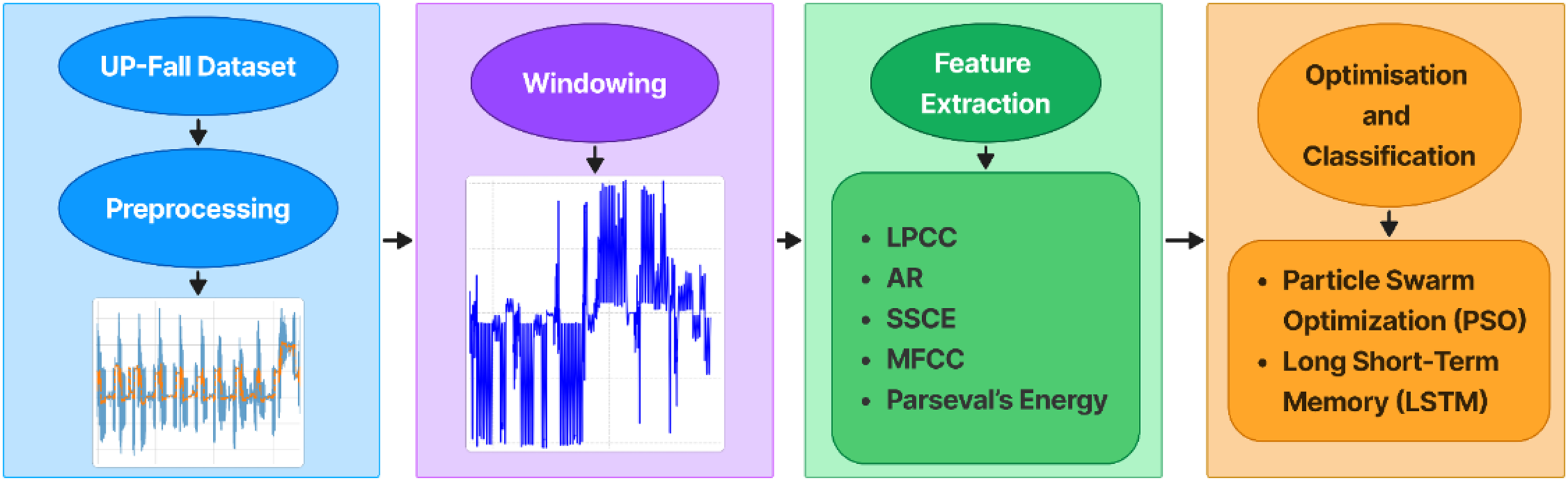
The human fall detection system uses inertial sensor data which requires pre-processing for data quality improvements. A Butterworth filter of the 6th order provides noise reduction and a Hamming window with a length of 10 s enables signal segmenting. To preserve transitional motion information while avoiding excessive redundancy, a fixed stride of 50% of the window length was utilized during segmentation, facilitating overlap between subsequent windows to retain transitional motion information while ensuring reasonable computational complexity. The subsequent phase applies SSCE coefficients and MFCC and LPCC features along with Parseval’s energy and AR coefficients. The feature detection methods include SSCE for signal complexity assessment and MFCC for spectral compactness as well as LPCC for temporal pattern identification and Parseval’s energy measurement of intensity plus AR coefficients for temporal relationships. The PSO optimization technique enhances the features by cutting down computational complexity through the selection of the most relevant features. An LSTM network functions by detecting temporal patterns to perform data classification operations. The process follows four distinct phases which include preprocessing and feature extraction together with optimization before the classification step, as illustrated in Fig. 1. Each stage is explained in detail throughout this text.
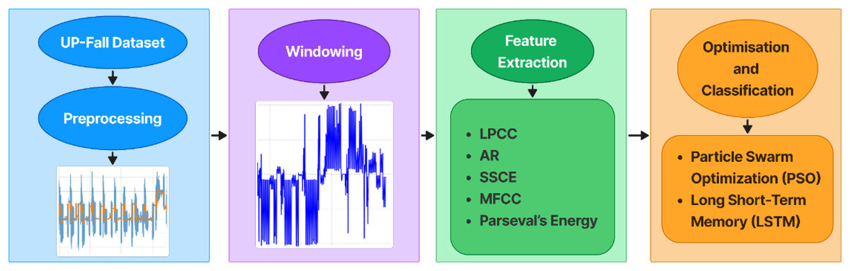
Figure 1: A comprehensive overview of the proposed fall actions detection system.
Pre-processing
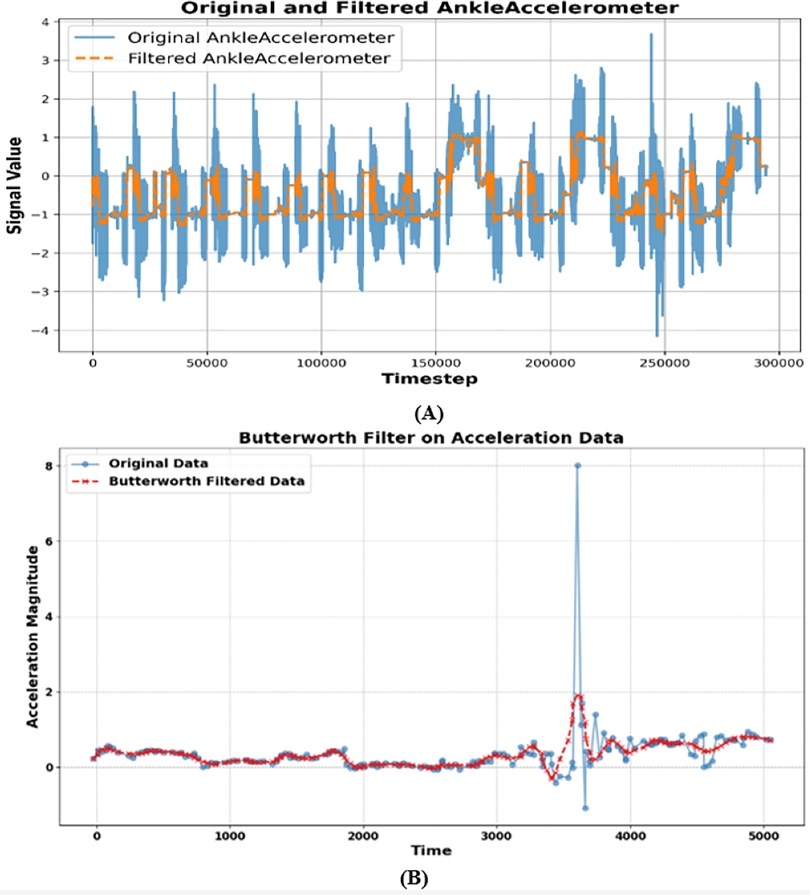
A sixth-order Butterworth low-pass filter executed preprocessing operations on inertial sensor data as a step for noise elimination. A Butterworth filter enables flat passband frequency response because it works well for systems demanding smooth response characteristics. The filter is defined by its order and cutoff frequency with the transfer function given by:
(1) where x is the complex frequency variable, is the cutoff angular frequency, and n is the filter order. In this study, a sixth order butterworth filter (n = 6) was used, with a cutoff frequency Hz. Given a sample rate of Hz, the Nyquist frequency was calculated as , resulting in a normal cutoff frequency of . This configuration effectively reduced high-frequency noise while preserving the underlying signal characteristics. The results of raw vs filtered data over both UP-fall and UR-fall datasets are shown in Figs. 2A and 2B.
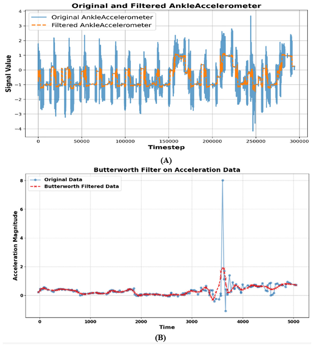
Figure 2: Results of preprocessing for the (A) UP-fall and (B) UR-fall datasets.
Windowing
The processed IMU sensor data received division into smaller parts using windowing approaches before additional examination. The research applications accessed these merged windows which were created after their overlapping process finished. Application of the Hamming window served to decrease spectral leakage effects while keeping data continuity throughout each divided section. The definition of the Hamming window exists as follows in mathematical format:
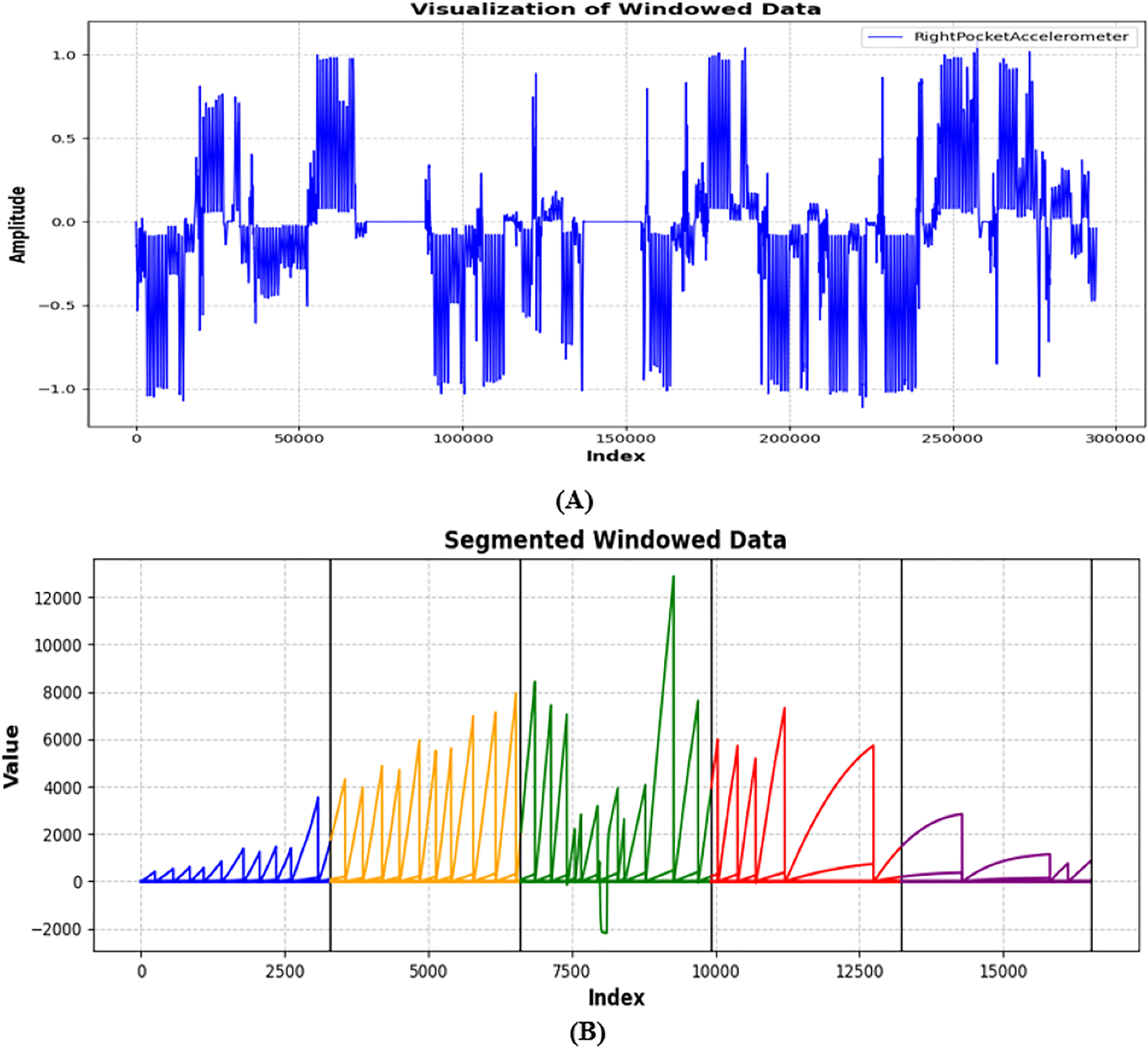
(2) where ranges from 0 to M-1, and M is the total number of samples in the window. A window size of 10 s (M = 1,000, assuming a sample rate of 100 Hz) was chosen as shown in Fig. 3. Hamming window filters performed sensor value transition smoothing during the segmentation process at the start and end of each window. The process of semantic segmentation was finalized by placing stacked windows with overlap to produce one seamless dataset for subsequent evaluation.
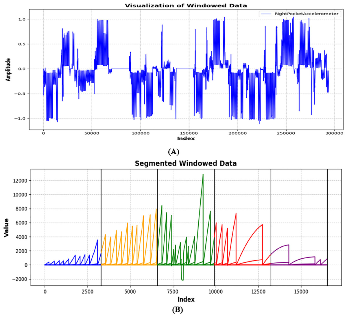
Figure 3: Signal windowing by applying Hamming windows for (A) UP-fall and (B) UR-fall dataset.
Feature extraction
The proposed system obtains several essential features from inertial data following data windowing. SSCE coefficients along with MFCC and LPCC and Parseval’s energy and AR coefficients form the set of extracted features. The upcoming subsections present an overview of the extraction process and evaluation outcomes for these features. The comparative analysis of techniques is shown in Table 2.
| Technique | Advantages | Limitations | Time complexity | Space complexity | Applicability |
|---|---|---|---|---|---|
| Butterworth 6th order filter | Smooth frequency response; Good noise suppression without distorting signal shape | Fixed cutoff; Not adaptive to changing signal noise | O(n) (single-pass filtering) | Low (stores few past samples & coefficients) | Ideal for IMU noise reduction before segmentation |
| Hamming window segmentation | Reduces spectral leakage; Maintains signal continuity | Window size fixed; May miss short transients | O(n) | Low (stores one window at a time) | Improves frequency domain analysis accuracy |
| SSCE | Captures signal complexity; Sensitive to temporal changes | Computationally more expensive than basic features | O(n2) (distance matrix computation) | Moderate (stores pairwise distances) | Good for distinguishing dynamic vs. static movements |
| MFCC | Captures spectral patterns; Robust to noise | Primarily designed for audio, needs adaptation for IMU | O(n·log n) (FFT + filter bank) | Moderate (stores filter bank coefficients) | Useful for activity pattern discrimination |
| LPCC | Models temporal signal dynamics well | Sensitive to noise if preprocessing is weak | O(n·p2) (where p = prediction order) | Low–Moderate | Complements spectral features with temporal info |
| Parseval’s energy | Simple to compute; Represents signal intensity | Cannot distinguish similar energy activities | O(n) | Very low | Effective for separating high/low intensity movements |
| Auto-Regressive (AR) coefficients | Good for repetitive motion modeling | Assumes linearity; May not capture complex dynamics | O(n·p) | Low | Suitable for modeling periodic motion in falls |
| Particle swarm optimization (PSO) | Reduces feature dimension; Improves classifier efficiency | Requires parameter tuning; May converge locally | O(k·n·d) (k = particles, d = dimensions) | Moderate (stores swarm states) | Boosts performance & reduces overfitting |
| LSTM classifier | Learns long-term dependencies; Handles sequential data well | High computation & memory; Needs GPU for speed | O(n·m2) (m = hidden units) | High (stores weights & states) | Best for complex temporal pattern recognition |
State space correlation entropy
By applying SSCE, researchers examined both the time-related structure and signal complexity to extract motion-related features. The analysis procedure divides signals into overlapping embedded vectors through a predetermined time delay system. The distance matrix requires two sets of pairwise vector comparisons which produce self-correlation information on the diagonal and vector distance readings between off-diagonal elements. The derived covariance matrix consists of distances that determines correlation probabilities leading to the computation of SSCE according to the following:
(3) where, and are the embedded vectors, represents the Euclidean distance between them, is small threshold, N is the total number of embedded vectors, and (x) is the Heaviside function. The computation of SSCE values for every data window allowed researchers to establish an average measure that describes motion signal complexity. The data points were organized according to activity categories and bar charts showed the SSCE values distribution throughout different activities of the dataset. This method extracts dynamic features from signals that lead to reliable insights about separating different activity types. Figure 4 represents results obtained from extracting SSCE from both datasets.
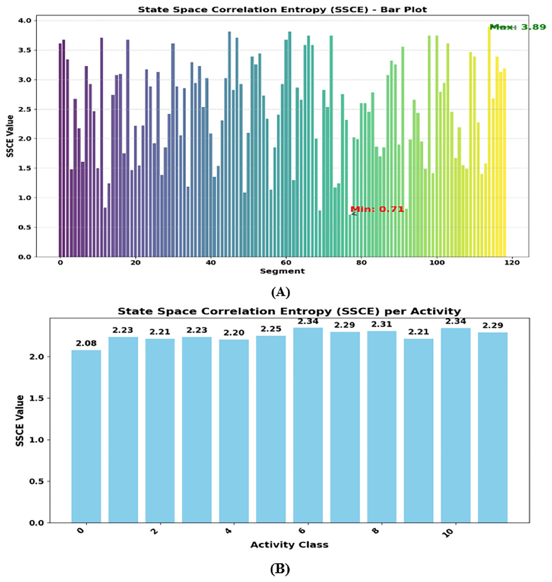
Figure 4: Extracted SSCE coefficients over (A) UP-fall and (B) UR-fall datasets.
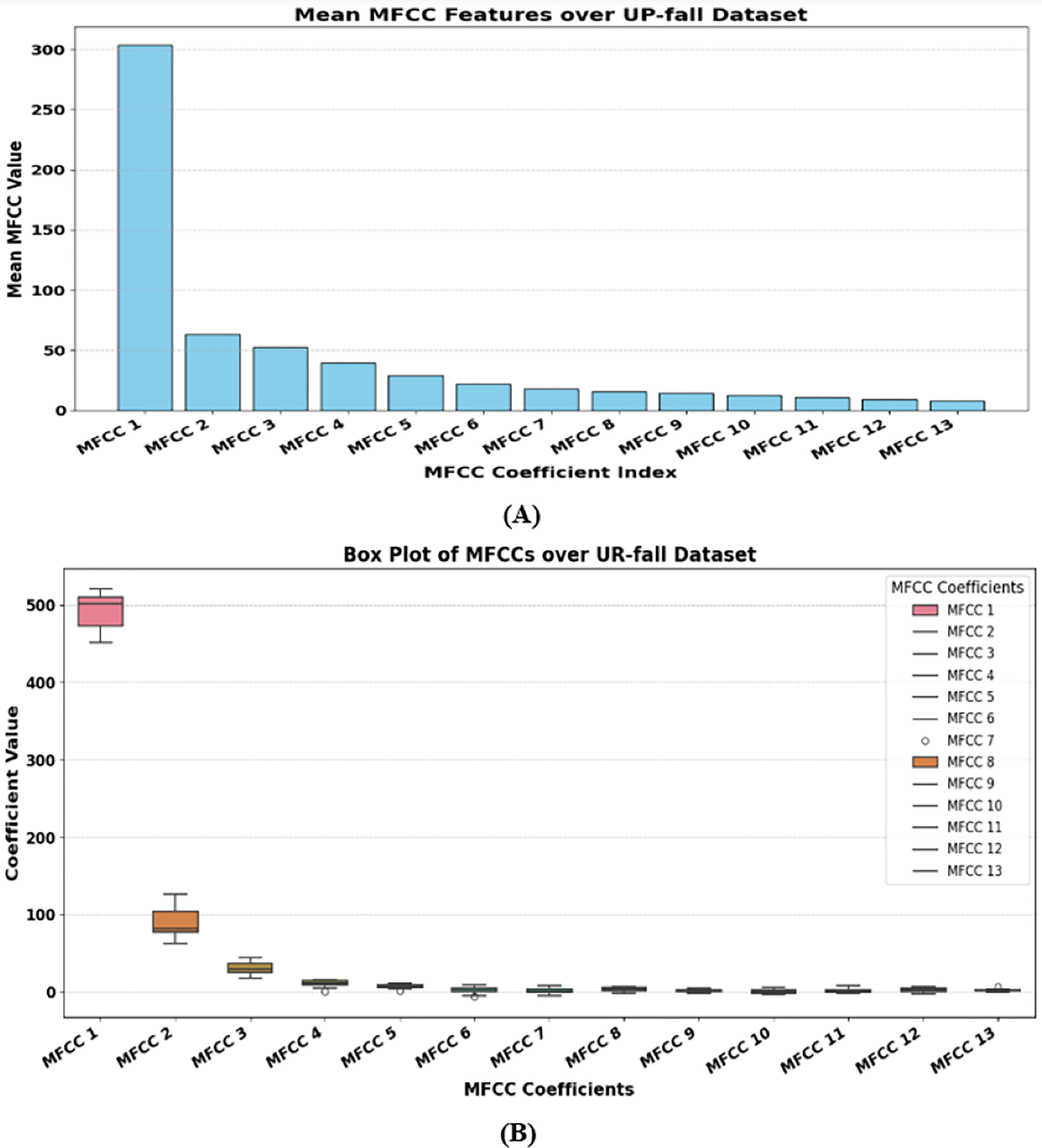
Mel frequency cepstral coefficients
The MFCC feature analyzes the spectral bands of inertial sensor data to extract spectral characteristics from the signal effectively. The information extraction occurs through peak identification of periodic components which transforms the signals into data that exists between time and frequency domains. The movement patterns get robust representation from MFCCs because they use sensor data to explain recorded signal changes. The MFCC feature is calculated using a discrete cosine transform, where the log filter bank amplitude is derived, and the total number of filter bank channels Q determines the final feature, as shown in the following equation.
(4)
Here shows the log filter bank amplitude, Q is the total number of filter bank channels, and r is the coefficient index. Due to their ability to detect frequency alterations in inertial data the MFCCs produce more precise activity pattern recognition. The Fig. 5 shows a visual display of MFCCs which corresponds to the Ankle Angular Velocity data within the sensor measurements.
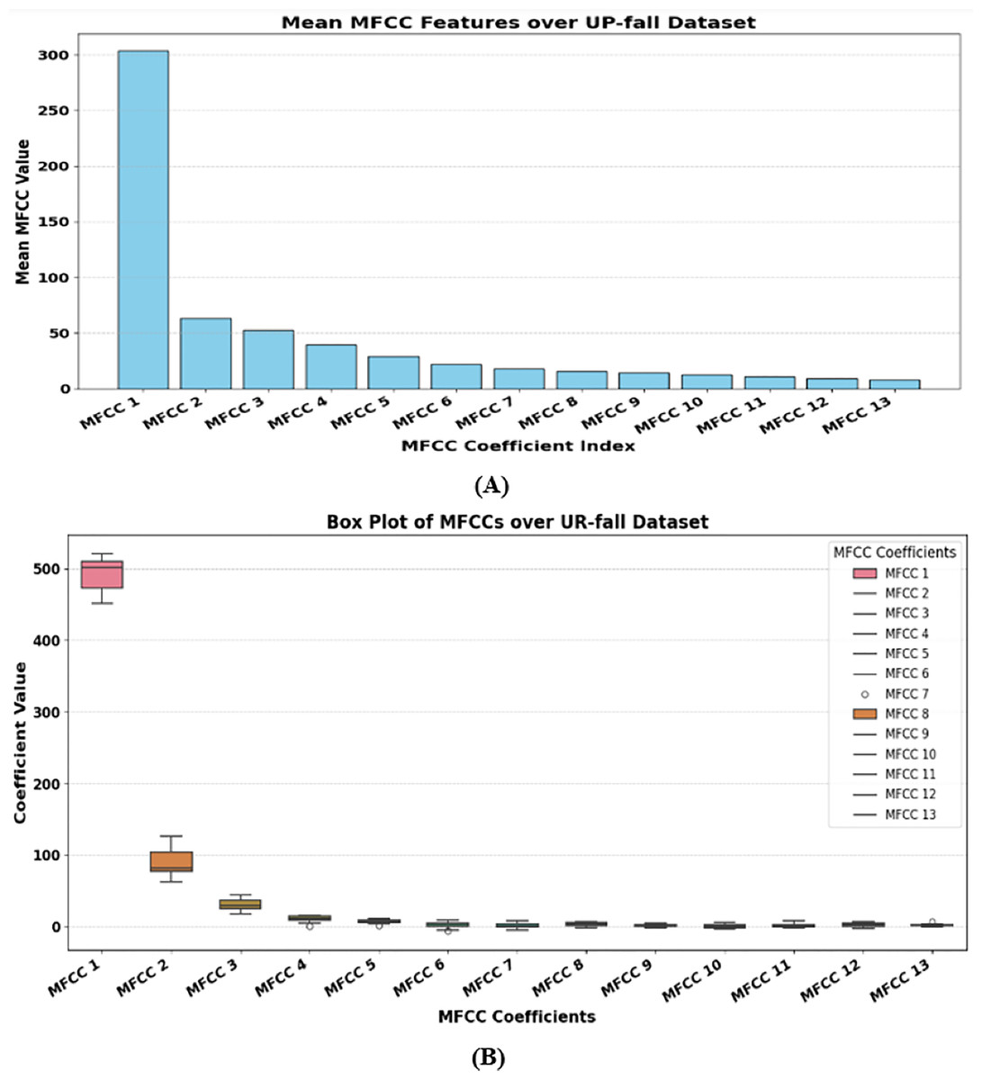
Figure 5: Mean MFCC values for (A) UP-Fall and box plot of MFCCs for (B) UR-Fall, showing coefficient distribution and variability.
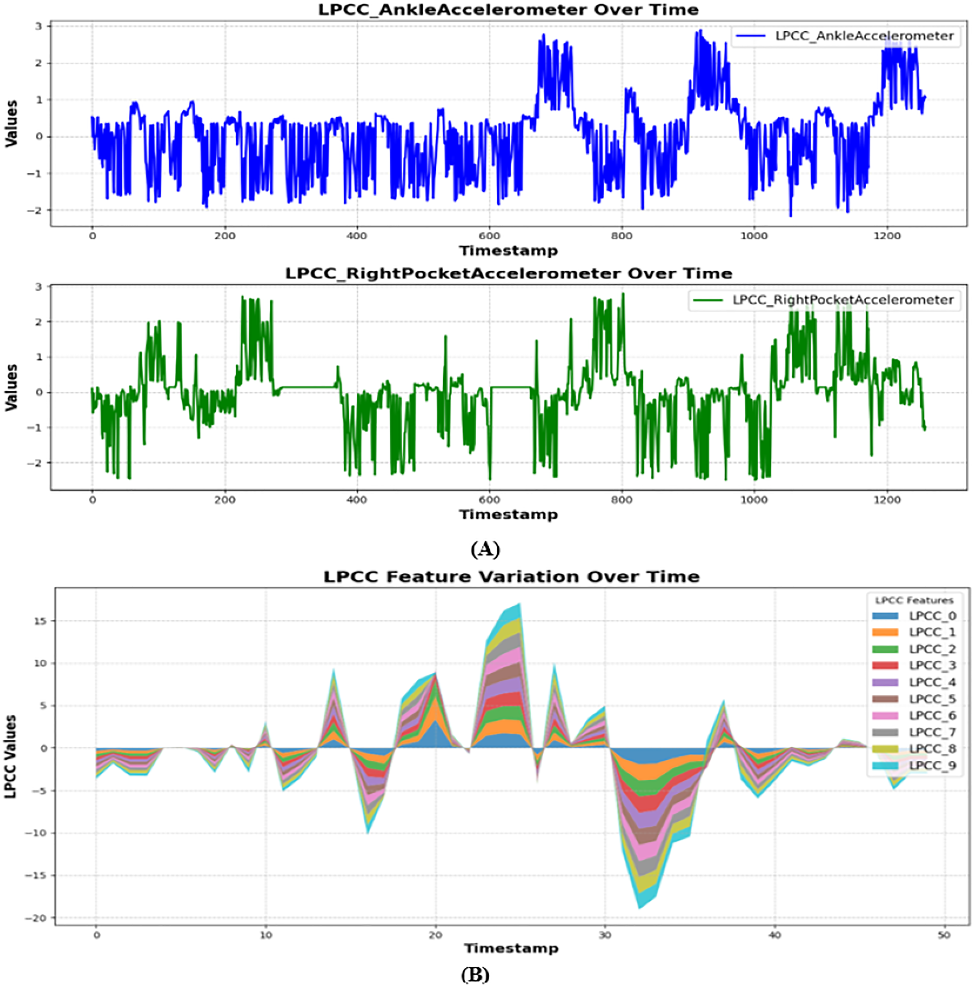
Linear predictive cepstral coefficients
The inertial signals produce LPCC features through a combination of signal transfer functions and first derivative analyses of specific frequency bands. The calculated coefficients describe signal movement patterns through sequential computations based on linear prediction coefficients b(m). Different equations determine the computation of LPCC coefficients:
(5)
(6)
Here, represents the LPCC coefficient. is the linear prediction coefficient, p is the prediction order. q is the total number of coefficients, and is the binomial coefficient. The cepstral coefficients are calculated per frame in each equation which results in powerful signal dynamics representations across time and frequency domains. LPC coefficients were computed with order 12 for the inertial signals from all their measurement axes in this research. Visual information about coefficient temporal dynamics appeared in time-series plots for features produced through the LPCC algorithm across the X, Y, and Z axes. The visual representations of LPCC data show their effectiveness in detecting movement patterns as they track signal variations continuously across various activities. An output presented in Fig. 6 represents the data extraction results from the dataset after performing LPCC processing.
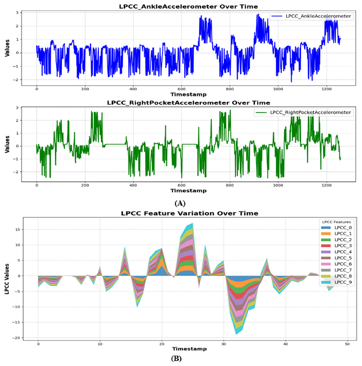
Figure 6: LPCC values of inertial data for (A) UP-fall from ankle, right pocket, and belt sensors over time and (B) UR-fall dataset.
Parseval’s energy
We determined the signal power strength through Parseval’s energy applied to accelerometer data windows during different activities. The calculated energy using Parseval’s theorem provides a precise measurement of the signal’s total power which exists in both the time domain and frequency domain. According to Parseval’s theorem, the signal energy measured in the time domain equals its energy values in the frequency domain. The formulation of time domain energy matches the definition of frequency domain energy as follows:
(7)
(8)
Parseval’s Theorem states that:
(9) where x(t) is the signal in the time domain. is its counterpart in the frequency domain, t represents time and shows the angular frequency. Parseval energy was then calculated for each window by summing the squared signal values within the window:
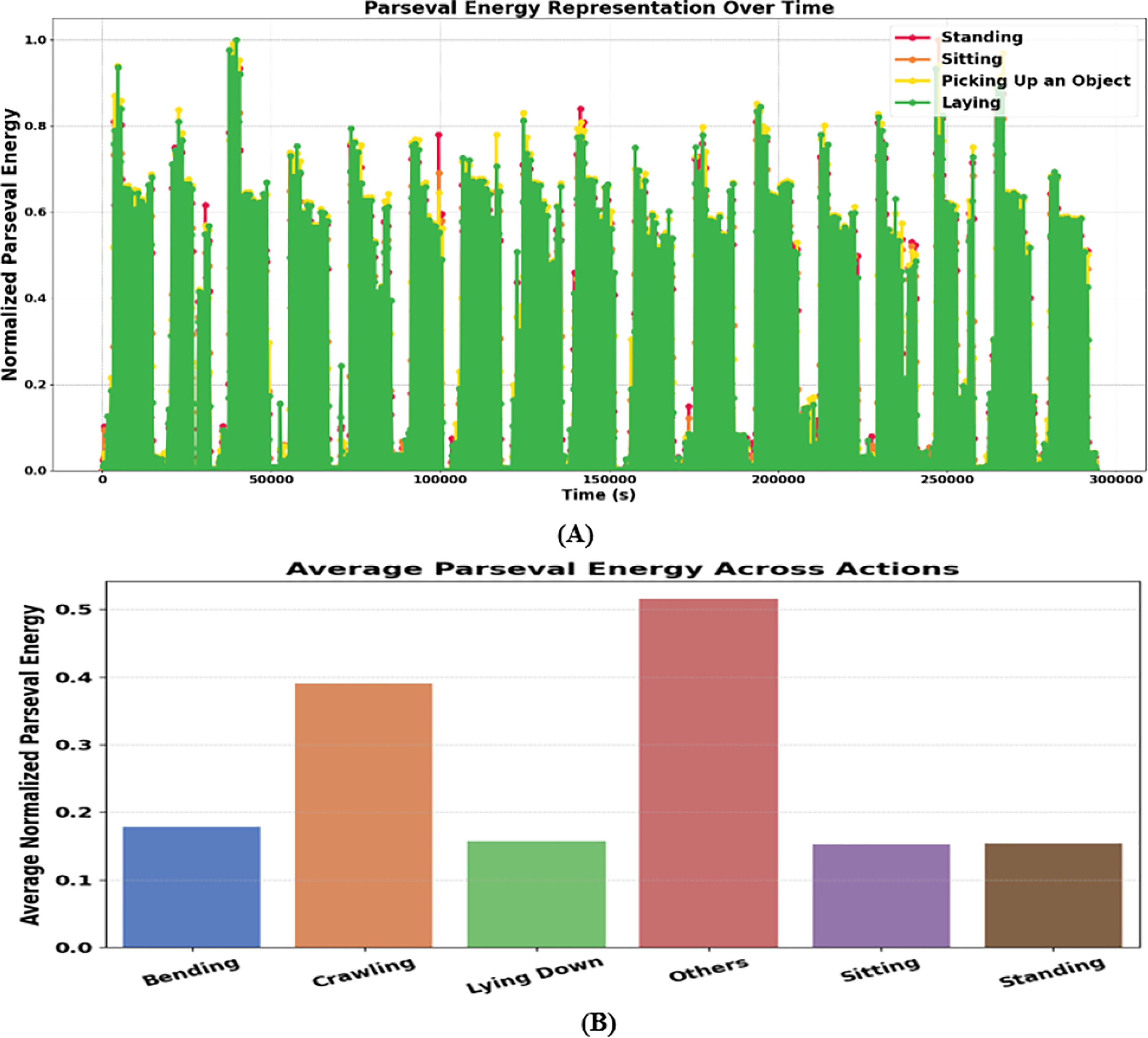
(10) where N is the number of samples in the window, and yk is the signal value at sample k. The calculated energies were normalized for visualization purposes, a subset of human activities has been plotted, as illustrated in Fig. 7A. The figure showcases the normalized Parseval’s energy distribution for selected actions, including standing, sitting, laying, and picking up an object over UP-fall dataset. The variations in energy levels across these activities highlight the distinctive characteristics of movement patterns, reinforcing the applicability of Parseval’s energy as a discriminative feature in activity recognition systems.
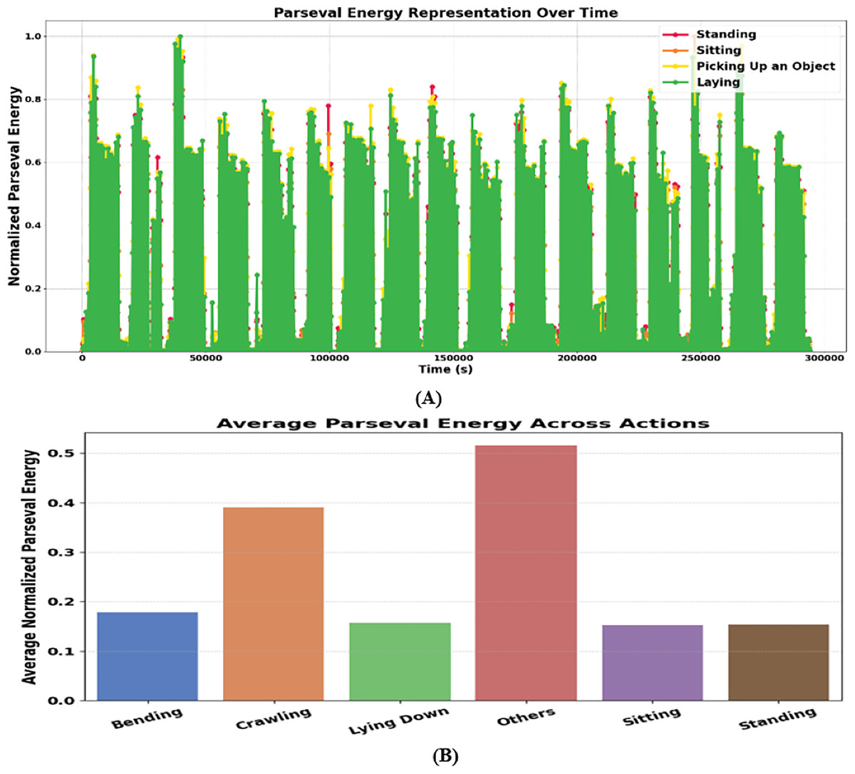
Figure 7: Normalized Parseval’s energy representation over time for selected activities (A) UP-fall and (B) UR-fall dataset.
Auto regression coefficients
The Auto-Regressive (AR) feature functions as a basic technical method that uses temporal relationships to examine repetitive motion patterns from sensor data. The model expresses each signal value through past observations weighted by autoregressive coefficients together with a dynamic error that adjusts to signal variation. A generalized AR model with an adaptive error component appears as follows:
(11) where represents past signal values, are autoregressive coefficients capturing temporal dependencies, is a noise component modeled as a moving average, are coefficients controlling the influence of past error terms, introduces a continuous memory effect through an exponential decay function, and is a weighting factor adjusting the contribution of historical patterns. Figure 8 displays the Auto regression plot for all the datasets.
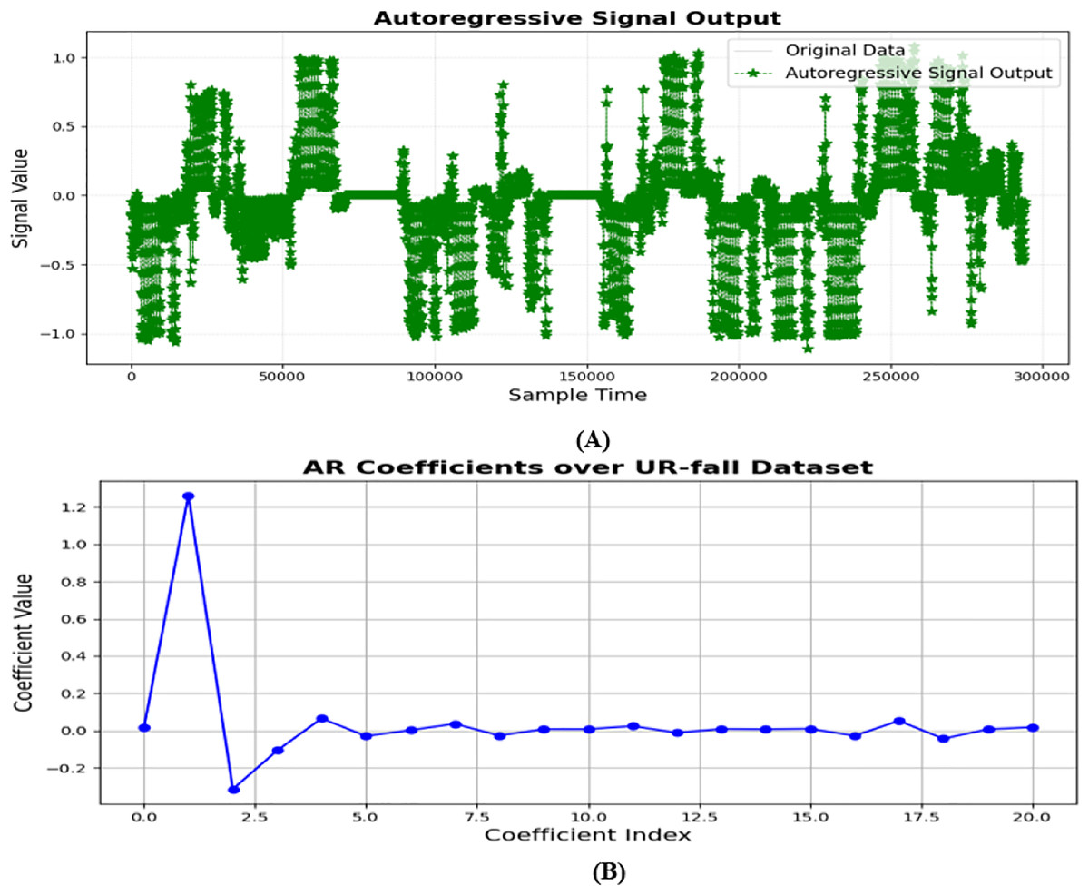
Figure 8: Autoregressive signal output demonstrating temporal dependencies in motion data for (A) UP-fall and (B) UR-fall dataset.
Particle swarm optimization
The population-based optimization algorithm Particle Swarm Optimization (PSO) derives its methods from active swarm psychology which mimics bird flocking and fish schooling behaviors (Batool, Jalal & Kim, 2019). This research uses PSO to optimize the selection of SSCE coefficient features combined with Parseval’s energy features as well as MFCC features LPCC features and AR coefficient features. Every swarm particle updates its position through its individual best experience together with the best positions located by the neighboring swarm members. The optimization process searches for minimum variance in weighted feature combinations that fulfill the requirement of total weight equality to one. This relationship appears as:
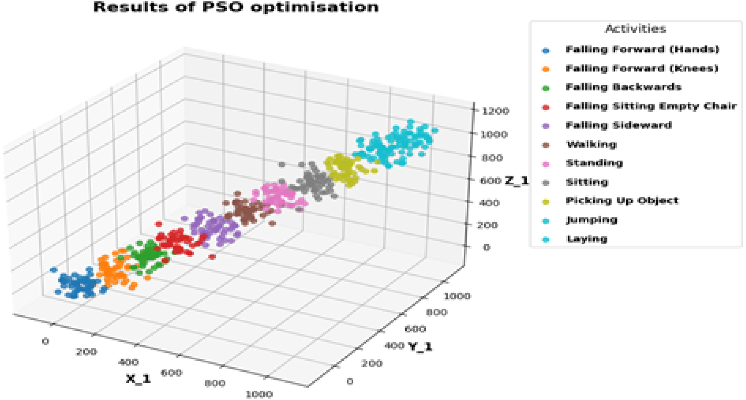
(12) where are the feature weights and are the extracted features. Through repeated updates of its weights, the PSO algorithm identifies an optimal data representation that enhances the performance of human fall action detection. The results of optimization over UP-fall dataset are shown in Fig. 9.
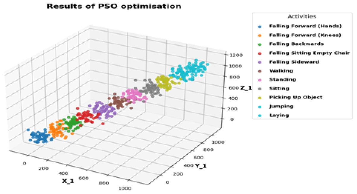
Figure 9: PSO optimization results over the UP-Fall dataset, illustrating activity-wise distribution in the reduced feature space.
Fall action classification
An LSTM network (Waheed et al., 2021) serves as the choice for fall action classification. LSTM represents a specialized RNN that excels at processing sequential data through its ability to detect longer-term dependencies thus making it appropriate for time-series classification tasks. The research uses UP-Fall and UR-fall datasets as input sources to extract SSCE coefficients together with Parseval’s energy and MFCC LPCC and AR coefficients from sensor signals. The classification performance receives enhancement through the use of Particle Swarm Optimization (PSO) for selecting essential features that promote discrimination. The model includes two stacked LSTM layers containing 64 units and 32 units which follow dropout regularization on fully connected layers to avoid overfitting. The final classification layer applies softmax activation to execute multiclass prediction because it works for the multiple action category prediction task. Standard scaling methods normalize the feature values while categorical results get encoded for preprocessing of both datasets. Training takes place with the Adam optimizer together with the categorical cross-entropy loss that follows this definition:
(13) where is the true label for class j, and denotes the predicted probability for that class. The research uses n-fold cross-validation instead of a train-test split for robust evaluation to test the model across multiple partitions of data.
Computing infrastructure
The experiments were conducted on a system equipped with an Intel Core i7-10510U CPU operating at 1.80 GHz (~2.3 GHz boost) with 8 cores and 8 GB of RAM. The system was running Windows 10 Pro (64-bit, Build 19045). The implementation and analysis were carried out using Python within the PyCharm integrated development environment (IDE). The data split for training and evaluation occurred through a n-fold cross-validation process. The proposed model delivered exceptional results on UP-fall and UR-fall benchmark dataset analysis. Additional information about database collection and assessment protocol is included in subsequent sections.
Datasets description
UP-fall dataset
The UP-fall detection dataset provides comprehensive data about identifying eleven fall-related activities (Martínez-Villaseñor et al., 2019) based on three trial executions from each subject. Healthy young people without disabilities participated in the dataset collection by performing eleven fall-related activities through wearable sensors and vision equipment with ambient sensors. The UP-fall detection dataset incorporates postures from six activities of daily living (ADL) which are standing (STD), sitting (STG), walking (WK), lying down (LA), jumping (JU), and picking up objects (PO) alongside five fall-related activities that include falling forward with hands (FH), falling forward with knees (FK), falling backward (FBK), falling sideways (FSD), and sitting on an empty chair (FEC) actions. The fall activities span 10 s yet the ADLs need 60 s of completion except for the jumping and object pickup which run for 30 s and 10 s, respectively.
UR-fall dataset
The UR fall detection dataset was created from data obtained through a combination of two USB-connected Kinect cameras and an IMU device which operated at the waist via Bluetooth connectivity. The ADL events were recorded using only Camera 0 as well as an accelerometer. The sensor data acquisition involved PS Move hardware and the x-IMU system. The study was conducted with five volunteers who performed 70 sequences among 30 fall-induced sequences and 40 sequences of ADL activities within an office setting. Each participant executed multiple forward (FF) and backward (FB) along with lateral falls onto the 2 cm thick carpet space with intended motions at least three times. The x-IMU sensor was operated by the researchers near the pelvic region. Participants performed the ADLs by standing (ST), sitting (SG), squatted, and bending (BG) their bodies after which they picked up objects and rested on the settee. Falls detected by the system demonstrated perfect accuracy but the sensor misidentified quick sitting activities (SG) because it confused them with true falls without additional sensor data. The provided dataset comprises falls that happen when someone is standing (FST) along with falls that take place during the sitting (FS) phase. Each dataset entry includes original accelerometer measurements that accompany depth images from two Kinect cameras as well as RGB image time sequences. A threshold-based fall detection technique served as one of the methods described by the researchers.
HealthLINK falls dataset
The HealthLINK Falls Dataset (Paolini et al., 2019) was gathered at the San Diego State University (SDSU) Neuromechanics and Neuroplasticity Laboratory utilizing sixteen Noraxon Inertial Measurement Unit (IMU) sensors positioned at designated anatomical sites on participating graduate students and faculty members. Every participant donned a virtual reality headset and traversed a linear pathway within a regulated laboratory setting. Falls were externally triggered by the sudden removal of a cloth sheet positioned on the floor in front of a mattress, resulting in fall, stumble, trip, or no-response incidents. The IMUs captured 183 kinematic parameters, encompassing joint orientation angles and limb accelerations, at a sampling frequency of 200 Hz. Subsequent to each trial, the recorded data were analyzed utilizing the Noraxon myoRESEARCH (MR3) program to categorize scenarios as either fall (1) or no fall (0), hence producing a binary classification dataset. This dataset encompasses both induced falls and normal ambulation situations, serving as a valuable resource for the development and assessment of machine learning-based fall detection systems.
Assessment metrics
Evaluation metrics serve as a means to assess the performance of the selected deep learning classifier, including accuracy, precision, and F1-score. Tables 3 and 4 presents these evaluation metrics derived from the experimental findings. In this study, accuracy was defined as the ratio of correctly classified samples to the total number of samples. The three metrics are formulated as follows:
(14)
(15)
(16)
| Cls | ST | SG | LD | BG | CR | WA | PR | OT | FF | FB | GC | FS | FST |
|---|---|---|---|---|---|---|---|---|---|---|---|---|---|
| ST | 93 | 2 | 1 | 1 | 0 | 1 | 0 | 0 | 1 | 0 | 0 | 0 | 1 |
| SG | 2 | 93 | 1 | 1 | 1 | 1 | 0 | 0 | 0 | 0 | 1 | 0 | 0 |
| LD | 1 | 1 | 94 | 1 | 1 | 1 | 0 | 0 | 0 | 0 | 1 | 0 | 0 |
| BG | 1 | 1 | 1 | 93 | 1 | 1 | 0 | 0 | 0 | 0 | 1 | 0 | 1 |
| CR | 0 | 1 | 1 | 1 | 94 | 1 | 0 | 0 | 0 | 1 | 0 | 0 | 1 |
| WA | 1 | 1 | 1 | 1 | 1 | 93 | 0 | 0 | 0 | 0 | 1 | 0 | 1 |
| PR | 0 | 0 | 0 | 0 | 1 | 0 | 96 | 1 | 0 | 0 | 0 | 1 | 1 |
| OT | 0 | 0 | 0 | 0 | 1 | 0 | 1 | 94 | 1 | 1 | 0 | 1 | 1 |
| FF | 1 | 0 | 0 | 0 | 0 | 1 | 0 | 1 | 94 | 1 | 0 | 1 | 1 |
| FB | 1 | 0 | 0 | 1 | 0 | 0 | 0 | 1 | 1 | 94 | 0 | 1 | 1 |
| GC | 0 | 1 | 1 | 1 | 0 | 1 | 0 | 0 | 0 | 0 | 94 | 1 | 1 |
| FS | 0 | 0 | 0 | 0 | 0 | 1 | 1 | 1 | 1 | 1 | 1 | 93 | 1 |
| FST | 1 | 0 | 0 | 0 | 1 | 0 | 0 | 1 | 1 | 1 | 1 | 1 | 93 |
| Cls | FH | FK | FBK | FEC | FSD | WK | STD | STG | PO | JU | LA |
|---|---|---|---|---|---|---|---|---|---|---|---|
| FH | 95 | 2 | 1 | 0 | 1 | 0 | 0 | 0 | 1 | 0 | 0 |
| FK | 1 | 95 | 1 | 1 | 1 | 0 | 0 | 0 | 0 | 1 | 0 |
| FBK | 1 | 1 | 96 | 1 | 1 | 0 | 0 | 0 | 0 | 0 | 0 |
| FEC | 1 | 1 | 1 | 95 | 1 | 0 | 0 | 0 | 1 | 0 | 0 |
| FSD | 1 | 1 | 1 | 1 | 95 | 0 | 0 | 0 | 0 | 1 | 0 |
| WK | 0 | 0 | 0 | 0 | 0 | 99 | 0 | 0 | 1 | 0 | 0 |
| STD | 0 | 0 | 0 | 0 | 0 | 1 | 98 | 0 | 0 | 1 | 0 |
| STG | 0 | 0 | 0 | 1 | 0 | 0 | 0 | 97 | 0 | 1 | 1 |
| PO | 1 | 0 | 0 | 1 | 0 | 1 | 0 | 0 | 96 | 0 | 1 |
| JU | 0 | 1 | 0 | 0 | 0 | 0 | 0 | 0 | 1 | 97 | 1 |
| LA | 0 | 0 | 0 | 0 | 0 | 0 | 0 | 1 | 0 | 1 | 98 |
Results
We assessed the proposed Fall action detection system utilizing two datasets: the UP-fall, UR-fall, and HealthLINK datasets. Table 3 presents the actual confusion matrix of the system operating on the UR-fall dataset, which achieved a mean accuracy of 93.62%. According to the UP-fall dataset attained a mean accuracy of 96.5%, as indicated in Table 4. While the Table 5, the accuracy for the HealthLINK dataset is 95.25. The results are displayed in Tables 3, 4, and 5 below.
| Class | Fall | No fall |
|---|---|---|
| Fall | 193 | 7 |
| No fall | 12 | 188 |
We use precision, recall and F1-score as evaluation parameters in our research. Tables 3, 4 and 5 show the confusion matrix of UR-fall, UP-fall and HealthLINK_Falls detection datasets, respectively. Whereas, Tables 6, 7 and 8 display classification report of all the three datasets. Table 9 presents a comparison with state-of-the-art (SOTA) methods.
| Classes | Precision | Recall | F1-score |
|---|---|---|---|
| ST | 0.92 | 0.93 | 0.93 |
| SG | 0.93 | 0.93 | 0.93 |
| LD | 0.94 | 0.94 | 0.94 |
| BG | 0.93 | 0.93 | 0.93 |
| CR | 0.93 | 0.94 | 0.94 |
| WA | 0.92 | 0.93 | 0.93 |
| PR | 0.98 | 0.96 | 0.97 |
| OT | 0.95 | 0.94 | 0.95 |
| FF | 0.95 | 0.94 | 0.95 |
| FB | 0.95 | 0.94 | 0.95 |
| GC | 0.94 | 0.94 | 0.94 |
| FS | 0.94 | 0.93 | 0.94 |
| FST | 0.90 | 0.93 | 0.92 |
| Average | 0.937 | 0.937 | 0.940 |
| Classes | Precision | Recall | F1-score |
|---|---|---|---|
| FH | 0.96 | 0.95 | 0.95 |
| FK | 0.95 | 0.96 | 0.95 |
| FBK | 0.96 | 0.96 | 0.96 |
| FEC | 0.96 | 0.96 | 0.96 |
| FSD | 0.98 | 0.96 | 0.97 |
| WK | 1.00 | 1.00 | 1.00 |
| STD | 0.99 | 0.98 | 0.98 |
| STG | 0.99 | 0.97 | 0.98 |
| PO | 0.98 | 0.99 | 0.99 |
| JU | 0.94 | 0.98 | 0.96 |
| LO | 0.98 | 0.98 | 0.98 |
| Average | 0.97 | 0.97 | 0.97 |
| Classes | Precision | Recall | F1-score |
|---|---|---|---|
| Fall | 0.94 | 0.96 | 0.95 |
| No fall | 0.96 | 0.94 | 0.95 |
| Average | 0.95 | 0.95 | 0.95 |
| Methods | UR-fall | UP-Fall | HealthLINK falls |
|---|---|---|---|
| Ghadi et al. (2022) | – | 95.00 | – |
| Hafeez et al. (2023) | 92.83 | 91.51 | – |
| Kwolek & Kepski (2015) | 90.00 | – | – |
| Le, Tran & Dao (2021) | – | 88.61 | – |
| Paolini et al. (2019) | – | – | 92.00 |
| Proposed system mean accuracy (%) | 93.62 | 96.5 | 95.25 |
Note:
The bold entries represent the accuracies achieved by the proposed method on the datasets used in this study.
Limitations
The established fall detection system utilizing wearable inertial sensors with deep learning capabilities operates effectively but encounters some performance limitations. A significant limitation arises from the system’s reliance on public statistics, which inadequately capture the diversity of sensor location, movement patterns, and subject characteristics. The incorporation of the HealthLINK_Falls dataset and the shank-mounted IMU dataset somewhat alleviates the demographic and sensor-placement limitations of the original UP-Fall and UR-Fall datasets; nonetheless, certain constraints persist. The UP-Fall and UR-Fall datasets consist of controlled, self-initiated falls by younger individuals, which may vary from inadvertent falls in older adults regarding reaction times, muscle strength, and postural stability. Despite the incorporation of more realistic fall simulations and better sensor placement in the new datasets, additional study including actual older people and real-world fall data is necessary to thoroughly capture age-specific motion patterns and enhance generalizability. Moreover, whereas shank-mounted recordings enhanced accuracy and F1-scores, practical implementation may be limited by user adherence and device configuration. The classification results presented in Table 5 exhibit high accuracy, precision, recall, and F1-scores under controlled experimental conditions utilizing the UP-Fall, HealthLINK_Falls dataset and UR-Fall datasets; however, these outcomes pertain solely to the tested scenarios and may not directly apply to uncontrolled real-world settings. The system’s success is contingent upon three primary factors: the internal noise levels of the sensors, their optimum location, and the necessity for optimal ambient conditions devoid of external interference. Moreover, the system demonstrates restricted ability to identify novel or unforeseen movement patterns due to its training being confined to established activity categories. These limitations align with difficulties noted in comparable wearable sensor systems and underscore the necessity of evaluating both empirical efficacy and practical implementation considerations. The system’s resilience and health monitoring applications will enhance when various data collection methodologies are integrated with adaptive learning methods and real-time optimization approaches.
Conclusion and future work
This work illustrates that the use of sophisticated preprocessing, varied feature extraction methods, and enhanced sequence modeling can significantly elevate the precision and dependability of fall detection using wearable sensors. The integration of time-domain features (e.g., AR coefficients) and frequency-domain features (e.g., MFCC, LPCC) offered complementary insights into motion patterns, while the PSO-driven feature selection markedly diminished redundancy, allowing the LSTM classifier to concentrate on the most distinguishing information. The outcomes on the UP-Fall and UR-Fall datasets demonstrated consistent improvements above baseline methods, validating the efficacy of this design decision. Nevertheless, the research underscored significant problems, including as sensitivity to sensor positioning, inadequate capture of real-world variability in benchmark datasets, and diminished generalization to novel activity categories. These observations highlight the necessity for adaptive learning methodologies, multimodal data integration, and extensive field testing to reconcile laboratory performance with real-world application in healthcare monitoring systems.
In future research, we will enhance the interpretability of the proposed fall detection system by incorporating explainable AI techniques such as Local Interpretable Model-agnostic Explanations (LIME) and SHapley Additive exPlanations (SHAP). These methodologies will clarify the influence of specific attributes and model decisions, similar to how local explanations have been used in intelligent healthcare systems for heart attack risk assessment to justify urgent treatment recommendations. Inspired by applications reported in “Enhancing Transparency in Smart Farming: Local Explanations for Crop Recommendations Using LIME” and “Role of Explainable AI in Crop Recommendation Technique of Smart Farming”, this integration will transform our LSTM-based framework from a non-transparent entity into a clear and trustworthy decision-support tool for healthcare environments.
We also aim to integrate self-attention mechanisms into the LSTM-based architecture to enable the model to focus on critical temporal segments and key feature interactions within inertial sensor data. This is expected to improve accuracy, robustness, and adaptability, leveraging the proven effectiveness of attention-based models in related domains. Further work will explore multimodal sensor fusion by combining inertial data with optical or depth sensing to improve detection reliability in varied conditions, as well as adaptive and online learning strategies to allow real-time parameter updates in response to changes in sensor placement, user movement patterns, or environmental factors. Additionally, we will focus on reducing model complexity for deployment on low-power edge devices, ensuring applicability in wearable and IoT-based healthcare systems. Comprehensive field testing with diverse populations, including older adults and individuals with mobility impairments, will be conducted to evaluate robustness, usability, and user acceptance in real-world scenarios.