
DeepFusion encoder for unsupervised monocular metric depth estimation
- Published
- Accepted
- Received
- Academic Editor
- Consolato Sergi
- Subject Areas
- Artificial Intelligence, Autonomous Systems, Computer Vision, Robotics, Software Engineering
- Keywords
- Monocular depth estimation, Self-supervised, Metric depth, Optical flow, Robot perception, Deep learning, Scene understand, Machine vision, Hierarchical context encoding, Monocular 3D perception
- Copyright
- © 2026 Huang et al.
- Licence
- This is an open access article distributed under the terms of the Creative Commons Attribution License, which permits unrestricted use, distribution, reproduction and adaptation in any medium and for any purpose provided that it is properly attributed. For attribution, the original author(s), title, publication source (PeerJ Computer Science) and either DOI or URL of the article must be cited.
- Cite this article
- 2026. DeepFusion encoder for unsupervised monocular metric depth estimation. PeerJ Computer Science 12:e3299 https://doi.org/10.7717/peerj-cs.3299
Abstract
Monocular depth estimation is a fundamental task in computer vision, with significant applications in autonomous driving and robotics. However, accurately estimating depth from a single image remains challenging due to the absence of direct depth cues. In this article, we present a novel self-supervised monocular depth estimation framework that integrates neural networks with multiscale 3D spatial loss to directly predict metric depth, thereby addressing the scale ambiguity inherent in monocular setups. Our approach introduces three key innovations: (1) an innovative integration of attention mechanisms within the hierarchical context encoding structure, which facilitates adaptive depth estimation; (2) the incorporation of kinematic scaling loss into continuous time frames for gradient backpropagation, significantly alleviating the scale ambiguity issue associated with monocular depth estimation; and (3) the construction of the University of Malaya Autonomous Driving (UMAD) dataset—an entirely original urban autonomous driving dataset created using Frequency-Modulated Continuous-Wave Light Detection and Ranging (FMCW LiDAR)—alongside methods for training, testing, and evaluation. Extensive experiments conducted on both the Karlsruhe Institute of Technology and Toyota Technological Institute at Chicago (KITTI) and UMAD datasets demonstrate that our method achieves substantial improvements in accuracy as well as real-time performance for depth predictions. Practical applications in monocular 3D perception further validate the effectiveness and robustness of our approach within autonomous driving scenarios.
Introduction
Monocular depth estimation has become increasingly vital for various computer vision applications, such as autonomous driving, robotics, and spatial intelligence. The evolution of monocular depth estimation techniques has enabled the practical integration of this approach into real-world engineering systems, particularly in autonomous driving platforms. For example, leading autonomous vehicles leverage this technology for 3D target perception, accurate scene reconstruction, vision-based localization, and critical safety decision-making, including obstacle avoidance and path planning. In complex traffic scenarios, monocular depth estimation supports robust environmental understanding, directly contributing to the reliability and safety of commercial autonomous driving solutions. These real-world deployments not only demonstrate its technical viability but also underscore its substantial research and application potential for next-generation artificial intelligent systems (Huang et al., 2025).
Although deep learning has significantly advanced the field of monocular depth estimation, the problem remains fundamentally ill-posed due to scale ambiguity. This challenge is particularly pronounced in dynamic scenes and for small objects, where the absence of reference scales complicates absolute depth recovery.
Traditional methods, often reliant on stereo geometry or multi-view setups, perceive the depth based on the various heuristic clues captured from a single perspective through experience. Common monocular depth clues include linear perspective (Dong et al., 2022; Tsai, Chang & Chen, 2005), focus/defocus (Tang, Hou & Song, 2015), atmospheric scattering (Guo, Tang & Peng, 2014), shadow (Yang & Shape, 2018), texture (Malik & Rosenholtz, 1997), occlusion and elevation (Hoiem et al., 2011; Jung et al., 2009).
In a multiview approach, the fundamental concept of structure from motion (SfM) is to deduce both camera movement and scene structure using multiview geometry (Bao & Savarese, 2011; Rublee et al., 2011; Davison et al., 2007). More recently, learning-based multi-view stereo (MVS) techniques utilizing deep 3D convolutional neural networks (CNNs) or transformer architectures have substantially improved dense scene reconstruction and depth estimation performance (Tong et al., 2024a, 2024b). For example, edge-assisted epipolar transformer networks achieve more reliable cross-view feature aggregation by leveraging both epipolar geometry and edge information, while parallax attention-based models enhance robustness in aerial scenes with large disparity variations. However, despite these advances, state-of-the-art MVS methods still face considerable challenges when deployed in complex real-world environments such as autonomous driving scenarios, which involve highly dynamic objects, rapid motion, and urban landscapes. In such situations, multi-view stereo may be unable to robustly handle occlusions or adapt in real time when only monocular video is available, limiting its suitability for practical perception requirements.
Most of the proposed deep learning methods for monocular depth estimation depend on supervised learning, which is based on ground-truth datasets during model training (Eigen, Puhrsch & Fergus, 2014; Eigen & Fergus, 2015; Cao, Wu & Shen, 2017; Kumar et al., 2018; Shao et al., 2023; Bartoccioni et al., 2023). This approach demands large-scale annotated datasets consisting of monocular images and corresponding depth values, which are expensive and often not feasible to acquire.
In response to this challenge, unsupervised methods have emerged as a promising approach, utilizing geometric constraints and photometric consistency to estimate depth from monocular sequences. The Monodepth framework (Zhou et al., 2017; Godard et al., 2019), a cornerstone in this domain, enables lightweight unsupervised depth estimation. Similarly, recent neural rendering and flow-assisted unsupervised multi-view stereo frameworks (Tong et al., 2025) further improve real-time monocular tracking and dense scene perception by integrating neural radiance fields and optical flow guidance, while alleviating the dependency on labeled data. Nevertheless, these unsupervised models are still constrained in their ability to predict metric depth due to the lack of absolute scale information, and often struggle to accurately estimate the depth of dynamic objects. This limitation is particularly critical for applications requiring precise depth measurements, such as obstacle avoidance in autonomous driving and assistive emergency braking (AEB) in level 2 advanced driver assistance systems (ADAS).
One prevalent approach in the current landscape involves predicting disparity maps by normalizing them through the median scaling ratio (Bhat, Alhashim & Wonka, 2021; Zhang, 2025). This method presents challenges in obtaining metric depth. Furthermore, existing network architectures primarily focus on estimating depth within static scenes. In practical and challenging scenarios that encompass dynamic scenes and complex geometries, it is essential to preserve inference speed without sacrificing precision (Laina et al., 2016; Godard, Mac Aodha & Brostow, 2017; Piccinelli et al., 2024). To address these challenges, we introduce a novel self-supervised monocular depth estimation framework that incorporates attention mechanisms and hierarchical context encoding. Simultaneously, the integration of kinematic scaling loss into continuous time frames facilitates gradient backpropagation. This innovative approach enables rapid and accurate absolute depth estimation in intricate environments.
Our method introduces three significant innovations:
-
An innovative integration of attention mechanisms within the hierarchical context encoding (HCE) divergent structure, allowing for adaptive parameter optimization that enhances feature representation. By incorporating spatial and channel attention layers, the network dynamically adjusts its focus on critical features at multiple scales, guided by the HCE module. This synergy not only improves the discriminating power of the extracted features but also optimizes the parameters to prioritize relevant spatial and contextual cues, leading to more precise and robust depth predictions.
-
Additionally, by utilizing a speed total loss function, we integrate kinematic scaling into continuous time frames for gradient backpropagation. This methodology penalizes the discrepancy between the model’s predicted velocity and the actual vehicle speed, effectively addressing the scale ambiguity issue commonly encountered in monocular depth estimation. Consequently, this approach results in more accurate and reliable metric depth maps.
-
The construction of the University of Malaya Autonomous Driving (UMAD) dataset—an entirely original urban autonomous driving dataset developed utilizing Frequency-Modulated Continuous-Wave Light Detection and Ranging (FMCW LiDAR), a monocular camera, and an inertial measurement unit (IMU) sensor—is presented alongside methodologies for training, testing, and evaluation.
As illustrated in Fig. 1, the predictions of our depth estimation model were compared with those generated by Monodepth2 (Godard et al., 2019) and Lite-Mono (Zhang et al., 2023). The results demonstrate that our model achieves superior accuracy in depth estimation for both moving vehicles and stationary small objects.
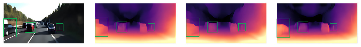
Figure 1: Qualitative Comparison.
(A) The original image data. (B) Our model, DeepFusion, demonstrates impressive performance in monocular depth estimation. The results indicate that our approach achieves superior accuracy in depth estimation for both moving vehicles and stationary small objects. (C) Results of monocular depth estimation using the Lite-Mono model. (D) Results of monocular depth estimation using the Monodepth2 model.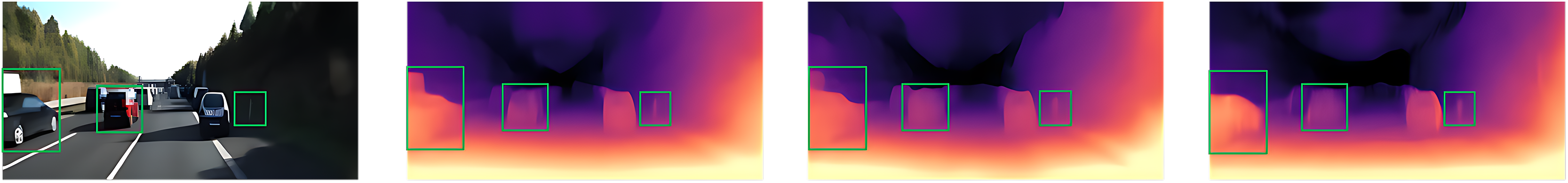
We conducted an evaluation of our method utilizing the Karlsruhe Institute of Technology and Toyota Technological Institute at Chicago (KITTI) (Geiger et al., 2013) and UMAD datasets for depth estimation and 3D perception tasks. The results indicate that the proposed approach not only enhances the accuracy of depth estimation across a diverse range of complex dynamic scenes but also facilitates the prediction of metric depth, representing a significant advancement for real-world applications. Furthermore, our accuracy experiments validate the effectiveness of each component, demonstrating that the integration of the fusion network, total speed loss, and optical flow substantially improves the overall performance of the model.
The structure of this article is organized as follows: ‘Related Work’ offers an overview of related work. ‘Methodology’ begins with essential preliminary knowledge and subsequently provides a comprehensive description of the proposed approach. Experimental results, accompanied by an in-depth discussion, are presented in ‘Experiments’. Finally, we conclude by addressing limitations and summarizing our findings.
Related work
Self-supervised depth estimation
Traditional depth estimation methods depend heavily on a substantial amount of labeled data for supervised learning (Kuznietsov, Stuckler & Leibe, 2017; Chen et al., 2016; Eigen & Fergus, 2015; Cao, Wu & Shen, 2017). However, acquiring depth labels in real-world scenarios is both challenging and costly, which has led to the rise of self-supervised learning approaches. In recent years, unsupervised deep learning has made remarkable advancements in monocular depth estimation, particularly when accurate depth labels are limited. Self-supervised methods present an effective solution for depth estimation tasks (Garg et al., 2016; Godard, Mac Aodha & Brostow, 2017). In the realm of self-supervised depth estimation, the most commonly used re-projection error is defined as , where the image synthesized from the depth map and camera pose is denoted as , while represents the target image. The re-projection error is optimized by minimizing the pixel differences between these images to refine depth estimation.
One of the commonly used methods in self-supervised depth estimation was based on stereo vision techniques, which achieved depth estimation through disparity map prediction (Li et al., 2024; Cheng, He & Zhang, 2018; Mo et al., 2023; Chen et al., 2021; Xia et al., 2024). In this approach, the model learns the disparity from the left image to the right image and uses geometric constraints to derive the depth map. , where is the baseline between the left and right cameras and is the focal length of the camera. The advantage of this method lies in its independence from explicit depth labels; relatively accurate depth maps can be generated through simple geometric transformations. However, this approach is contingent upon the use of a stereo camera system, where the horizontal distance b between the two monocular cameras must be meticulously calibrated; any inaccuracies in this measurement can adversely affect the precision of depth estimation. In practice, such precision may be significantly compromised by factors such as vibration and deformation, resulting in substantial deviations. To mitigate these discrepancies, recalibration is essential. Although online calibration methods are currently available, their accuracy remains uncertain, which imposes certain constraints on practical applications.
With the advent of monocular depth estimation methods, researchers have increasingly explored self-supervised learning approaches within monocular video sequences by leveraging temporal contextual information. A prominent example of these approaches is based on view synthesis. These methods predict the relative pose between the current frame and its adjacent frames, utilizing the depth map to synthesize images from alternative viewpoints. The model’s training objective is to minimize the re-projection error between the synthesized image and the actual image, thereby eliminating the necessity for direct use of depth labels during training. The article “Unsupervised Learning of Depth and Ego-Motion from Video” (Zhou et al., 2017) was pivotal in opening this field, leading to several subsequent enhancements aimed at improving performance. Notable advancements include the introduction of more sophisticated geometric models and a 3D convolutional depth estimation framework designed to enhance depth prediction accuracy (Casser et al., 2019; Zhang, Zhang & Tao, 2022; Bian et al., 2019). With the advancement of deep neural networks, self-supervised depth estimation methods have undergone significant evolution. Researchers are increasingly exploring ways to incorporate additional sources of information and semantic data within the self-supervised framework to enhance both the accuracy and robustness of depth estimation (Zhang, Zhang & Tao, 2022; Chen et al., 2019; Clark et al., 2017). These advancements suggest that self-supervised depth estimation can achieve performance levels comparable to those of supervised learning, all without relying on costly labeled datasets.
Metric monocular depth estimation
Depth estimation from monocular camera poses can be accomplished through various methodologies. Triangulation involves matching feature points across images and utilizing camera poses to compute three-dimensional (3D) points. Structure-from-motion (SfM) reconstructs 3D scenes by detecting features, estimating camera poses, and triangulating points across multiple frames (Lou & Noble, 2024; Guo et al., 2025). Optical flow estimates depth by analyzing pixel motion between frames in conjunction with camera movement, while disparity calculates depth based on pixel differences, focal length, and baseline distance (Teed & Deng, 2020; Shao et al., 2022). The selection of a particular method is contingent upon the specific application and the data available. However, in practice, these methods are often influenced by scene complexity and noise levels, which can result in diminished estimation accuracy. With the advancement of deep learning, metric depth estimation methods that leverage deep neural networks have gradually emerged. These approaches typically involve the integration of additional sensor data or specific training strategies to learn the absolute depth scale (Park, Kim & Sohn, 2019; He et al., 2024; Wang et al., 2024). For instance, certain studies combine LiDAR data with visual information, utilizing the depth measurements provided by LiDAR to calibrate the scale of depth estimation and thereby achieve precise metric depth estimation. However, this methodology also presents several drawbacks, including the high costs associated with LiDAR sensors, increased system complexity, and potential performance degradation (e.g., calibration accuracy), which collectively limit its widespread applicability.
In the field of depth estimation, metric monocular depth estimation seeks to directly derive depth maps with an absolute scale from a single image (Piccinelli et al., 2024; Zhang, Zhang & Tao, 2022; Wofk et al., 2023). Unlike traditional relative depth estimation methods, this approach requires the capability to determine actual distances between objects and the camera by integrating sensor information. This ability is essential for various practical applications, including autonomous driving and robotic navigation. However, due to vehicle vibrations and complex external environments, scaling models often encounter difficulties in accurately adapting to these conditions. As a result, discrepancies in computed outcomes emerge, posing challenges in ensuring precision in depth estimation.
Self-supervised absolute depth estimation methods have not been extensively researched or widely implemented, primarily due to challenges associated with guaranteeing their accuracy and generalization capabilities. These limitations hinder their effectiveness in real-world scenarios. The strength of this approach lies in its capacity to utilize a vast number of unlabeled images for learning purposes, thereby eliminating the need for costly annotated data and reducing data acquisition expenses. Nevertheless, accuracy may be compromised by variations in scene dynamics and lighting conditions that can negatively impact the reliability of depth estimation.
To address these challenges, our approach incorporates kinematic geometric constraints between image frames, along with integrated metric scale information that includes motion cues such as vehicle speed, acceleration, and angular velocity. This enhancement significantly improves both the accuracy and robustness of absolute depth estimation.
Depth estimation of dynamic objects
Self-supervised monocular depth estimation relies on the geometric consistency between frames, where static scenes enable more accurate pixel matching. However, the presence of dynamic objects compromises this assumption by introducing displacements that are independent of self-vehicle motion. As a result, the model encounters difficulties in establishing reliable correspondences for moving objects, often leading to erroneously inflated depth predictions that diverge toward infinity.
To tackle this challenge, various methodologies have been investigated. One such approach is the automask technique, which analyzes pixel information between frames to identify moving objects and subsequently excludes them from depth estimation (Zhou et al., 2017). While this method enhances accuracy for static objects, it constrains the ability to estimate depth for dynamic entities. Deep learning approaches utilize convolutional neural networks (CNNs) to identify dynamic objects and estimate depth based on the global context of a scene (Cheng, He & Zhang, 2018). While these methods are capable of learning intricate depth relationships from large datasets, they often demand substantial computational resources and extensive labeled data. Graphical model approaches, as exemplified by Vogel, Schindler & Roth (2013), capture the motion trajectories of dynamic objects to facilitate depth estimation. Although effective in managing motion relationships, these models can become complex and computationally intensive, particularly in highly dynamic environments. Recent advancements in neural radiance fields (NeRFs) have expanded their capabilities to encompass dynamic scenes, thereby enabling the depth estimation of moving objects. NeRF-based methods, such as those proposed by Li et al. (2021) and Park et al. (2021), employ implicit neural representations to model both static and dynamic components within a scene. By learning a continuous volumetric representation of the environment, these methods can estimate the depth of dynamic objects without necessitating explicit motion segmentation. However, NeRF-based approaches frequently encounter challenges related to real-time performance due to their computationally demanding rendering processes. Furthermore, they require dense multiview input and may struggle to generalize effectively to unseen motion patterns or highly occluded scenes (Tretschk et al., 2021).
In response to these limitations, this study proposes a novel approach that integrates optical flow geometric methods with multi-scale adaptive neural networks. The depth decoder is designed to progressively transform high-level feature representations generated by the encoder into dense depth maps through multiple upsampling stages. By effectively incorporating multi-scale contextual information from the encoder, the decoder can merge fine-grained details with a comprehensive understanding of the global scene, resulting in depth predictions that are both accurate and robust. The depth decoder employs skip connections from corresponding layers of the encoder. These connections ensure that high-resolution details from earlier layers are preserved and integrated into the final depth map. This method significantly enhances the accuracy of depth estimation and effectively addresses challenges associated with estimating depth for dynamic entities.
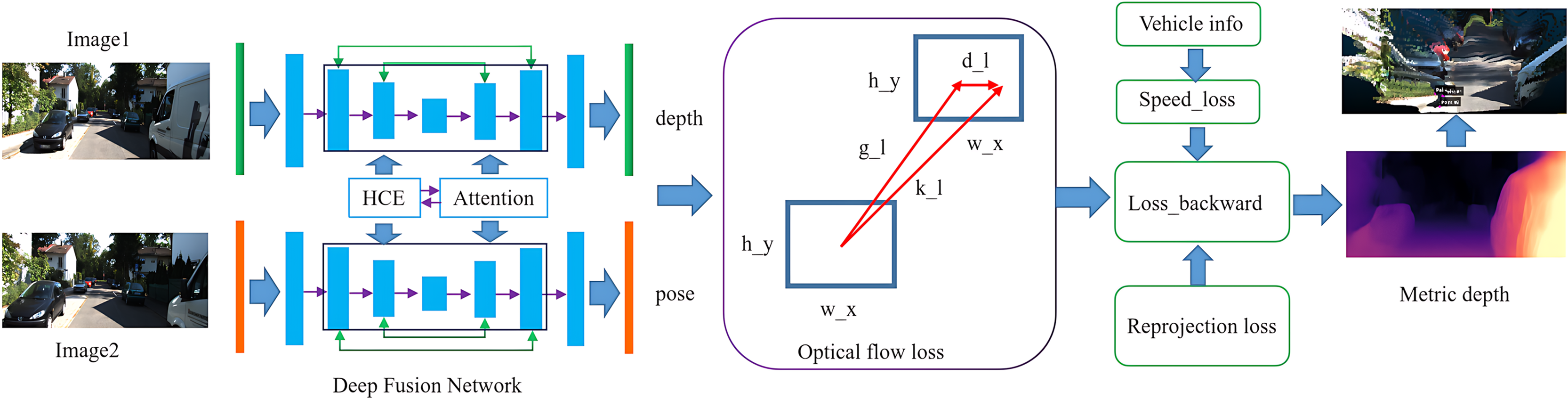
Figure 2 illustrates our framework pipeline. It presents consecutive raw image frames acquired from the camera. A deep fusion network is employed as our backbone, enhancing both efficiency and accuracy. The optical flow loss is utilized for estimating depth in dynamic scenes. We incorporate reprojection loss and speed loss to facilitate metric depth estimation. The final output includes the depth estimation result, represented as a disparity map, along with point cloud data derived from this disparity map.
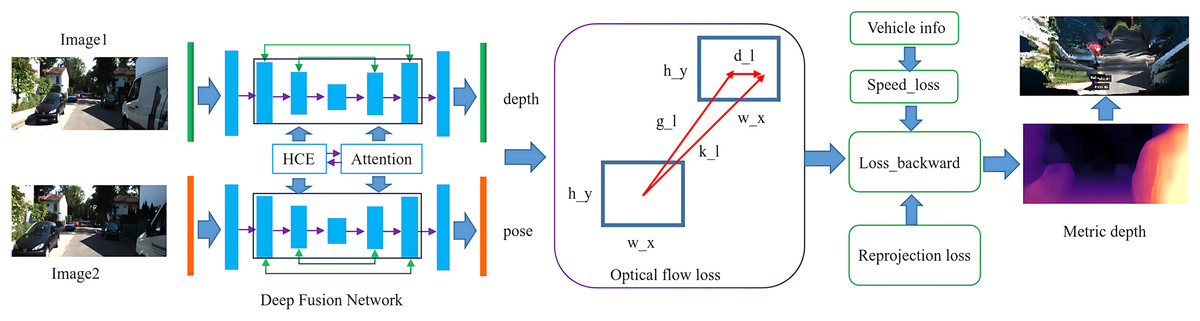
Figure 2: Framework pipeline.
The proposed approach utilizes hierarchical context encoding (HCE), which extracts features at multiple scales through the application of multi-scale convolutions. The feature attention module is employed on the combined feature maps generated by the hierarchical context encoding module. To further enhance representation, a global feature aggregation layer captures the overall scene context and conveys this information to the decoder. This facilitates dynamic, geometry-aware decoding that sharpens geometric details and improves boundary accuracy, ultimately resulting in the generation of four multi-scale inverse depth maps. In parallel, we integrate an optical flow decoder to predict dense motion fields, thereby introducing dynamic constraints that further refine depth estimation precision. By amalgamating multiscale context encoding, comprehensive scene understanding, and motion-guided constraints, our architecture achieves robust and highly accurate depth estimation.
Methodology
In this section, we first present the foundational knowledge essential for comprehending our work. Subsequently, we detail our novel contributions: an innovative convolutional neural network that integrates a hierarchical context encoding module, and a technique for absolute depth estimation designed with speed supervision in mind. Finally, we introduce an advanced autonomous driving dataset that we have established.
Preliminaries
In this section, we provide an overview of reprojection loss, optical flow, and the commonly employed loss functions within the context of monocular depth estimation.
Per-pixel minimum reprojection loss
The primary supervisory signal in self-supervised depth estimation is derived from the re-projection error. Specifically, the network generates a depth map for the target frame, while PoseNet estimates the relative camera pose between adjacent frames. By utilizing the estimated depth and pose, points from the target frame are projected into the source frame to ascertain their corresponding pixel coordinates. The pixel values at these locations are subsequently sampled from the source frame to reconstruct the target frame. The discrepancy between the original and reconstructed target frames—termed as re-projection error—serves as supervision for training the network.
For depth estimation, backpropagation calculates the gradient of the loss function with respect to the network parameters and updates the parameters to minimize the prediction error. Given a loss function L, which measures the error between the predicted depth and the ground truth, the network parameters are updated by computing the gradient of L with respect to :
(1) Regarding Eq. (1), is the input feature map, is the convolution filter.
Using the chain rule, backpropagation propagates this gradient through each layer of the network, iteratively updating the parameters via gradient descent.
(2) where is the learning rate. This update minimizes the loss, improving the accuracy of depth predictions.
From target frame to the camera coordinates
Starting with the red-green-blue (RGB) image at the target frame, the pixel coordinates and the estimated depth , which from the depth estimation network, allow us to map 2D points to 3D camera coordinates:
(3) In Eq. (3), K is the intrinsic matrix of the camera and is the 3D point in the camera coordinate system.
PoseNet estimates the relative pose between the target frame and the source frame by predicting the rotation matrix R and the translation vector . This allows us to transform the 3D points from the target frame to the source frame:
(4) Here, represents the 3D point transformed into the source frame.
Warping to the source frame
Using the predicted depth and pose, the corresponding pixel coordinates in the source frame can be computed. After obtaining the projected points, we warp the source image onto the target image plane.
(5) Here, are the projected pixel coordinates in the source image and Z is the depth value in the camera coordinate system.
The re-projection loss measures the similarity between the warped source image and the target image. This loss combines structural similarity (SSIM) and pixel-wise loss:
(6) The goal is to minimize this loss, ensuring that the projected image from the source aligns well with the target image. As with the backpropagation function and the estimated depth , if we minimize the loss , it means that the estimated depth is minimized, so we can obtain a more accurate depth estimation.
Optical flow loss
In depth estimation methods that rely on reprojection error, a fundamental assumption is that the camera moves while the scene remains static. This allows for effective error analysis between frames. However, in real-world scenarios, dynamic objects disrupt this assumption, resulting in inaccuracies due to their motion hindering consistent matching across frames (Yin & Shi, 2018; Shao et al., 2022; Ranftl, Bochkovskiy & Koltun, 2021; Fu et al., 2018; Poggi et al., 2020). Existing solutions often attempt to mitigate this issue by masking out moving objects; however, such approaches may overlook the multitude of dynamic entities present in environments like roadways (Godard et al., 2019; Guizilini et al., 2020). Our proposed method addresses this challenge by introducing an optical flow loss function that accounts for the motion of dynamic objects, thereby enabling robust depth estimation in these complex settings.
Optical flow represents the pixel-wise motion between frames, estimating a 2-D displacement vector field, , where and are the horizontal and vertical motion components, respectively. Given the brightness constancy assumption (Lucas & Kanade, 1981), which states that pixel intensity remains constant during movement, the optical flow constraint equation is derived as:
(7) where and represent the spatial image gradients, is the temporal gradient between frames.
Where and represent the spatial image gradients, is the temporal gradient between frames. To estimate optical flow, the network minimizes the photometric differences between consecutive frames, thereby facilitating pixel-wise motion learning. This approach enhances the accuracy of depth estimation in dynamic scenes.
Edge-aware smoothness loss
Edge-aware smoothness loss ensures that the depth map is smooth in regions where the image is smooth, while preserving edges where the image has strong gradients. The formula for this loss is the following.
(8) where represents the depth in the pixel , and represents the intensity of the corresponding image pixel. The exponential terms lower-weight the smoothness penalty in regions with strong image gradients, allowing for sharp depth discontinuities at object boundaries.
Affine invariant loss
To address variations in scale and camera motion, we introduce an affine invariant re-projection loss. This loss function is designed to align images by applying an affine transformation to the predicted depth map, thereby accommodating scene changes resulting from camera movement or object dynamics (Teed & Deng, 2020; Janai et al., 2018; Jeong et al., 2022; Liu et al., 2019; Bailer, Taetz & Stricker, 2015; Bar-Haim & Wolf, 2020). The definition of the affine invariant loss is as follows:
(9) where is the affine transformation matrix between frames and , optimized during training to minimize the error. This approach enhances the model’s robustness to scale variations and improves its capacity to capture dynamic changes within the scene. By jointly optimizing these loss functions, the model is able to generate more accurate depth maps, maintain temporal consistency across frames, and effectively adapt to dynamic environments. The integration of these combined losses ensures reliable performance in both static and dynamic scenes, ultimately leading to more precise and robust depth estimation.
Innovative convolution neural network
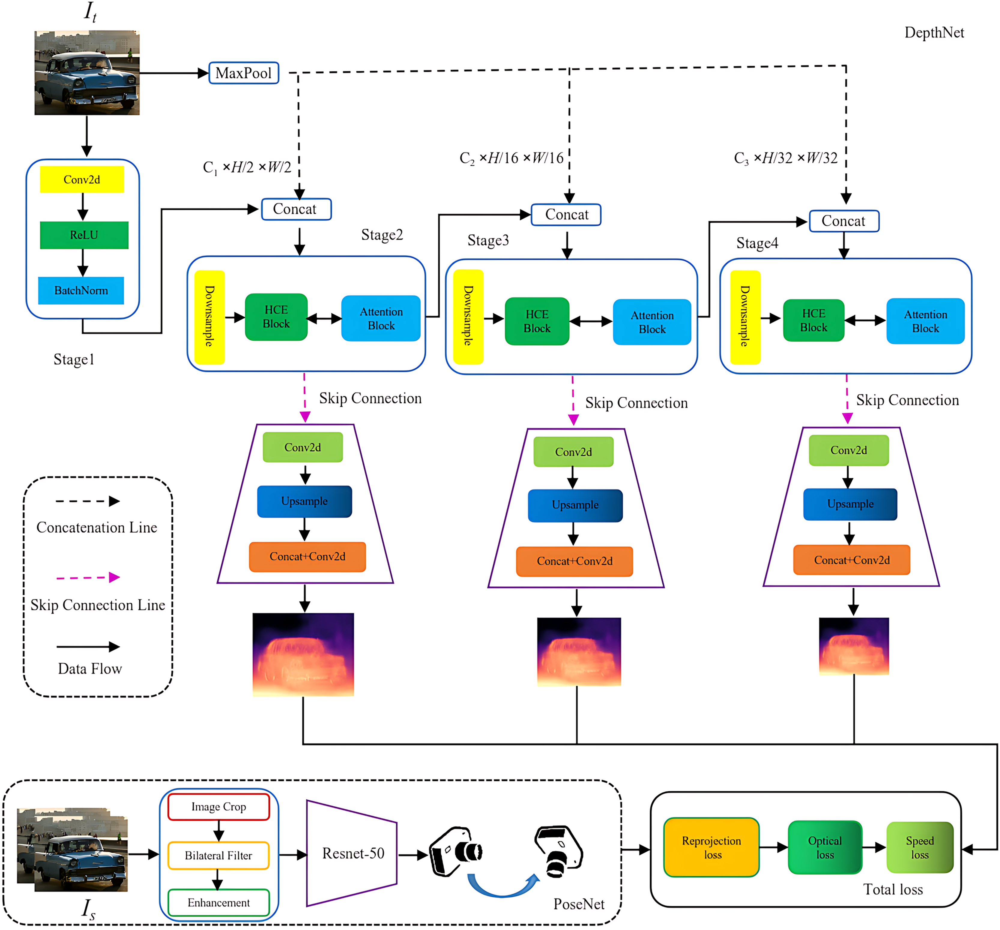
Previous research has primarily focused on improving the accuracy of depth estimation by emphasizing the volume and quality of supervised data, as well as the complexity of neural network architectures. This study aims to develop a network capable of effectively capturing both global context and fine-grained details within images while ensuring real-time inference. As illustrated in Fig. 3, the proposed framework consists of an encoder-decoder architecture referred to as DepthNet, along with a PoseNet module. The DepthNet is responsible for generating inverse depth maps at multiple scales from input images, whereas the PoseNet predicts the relative camera pose between consecutive frames. Subsequently, the model reconstructs the target image and computes a loss function to guide learning, ultimately facilitating the estimation of absolute-scale depth.
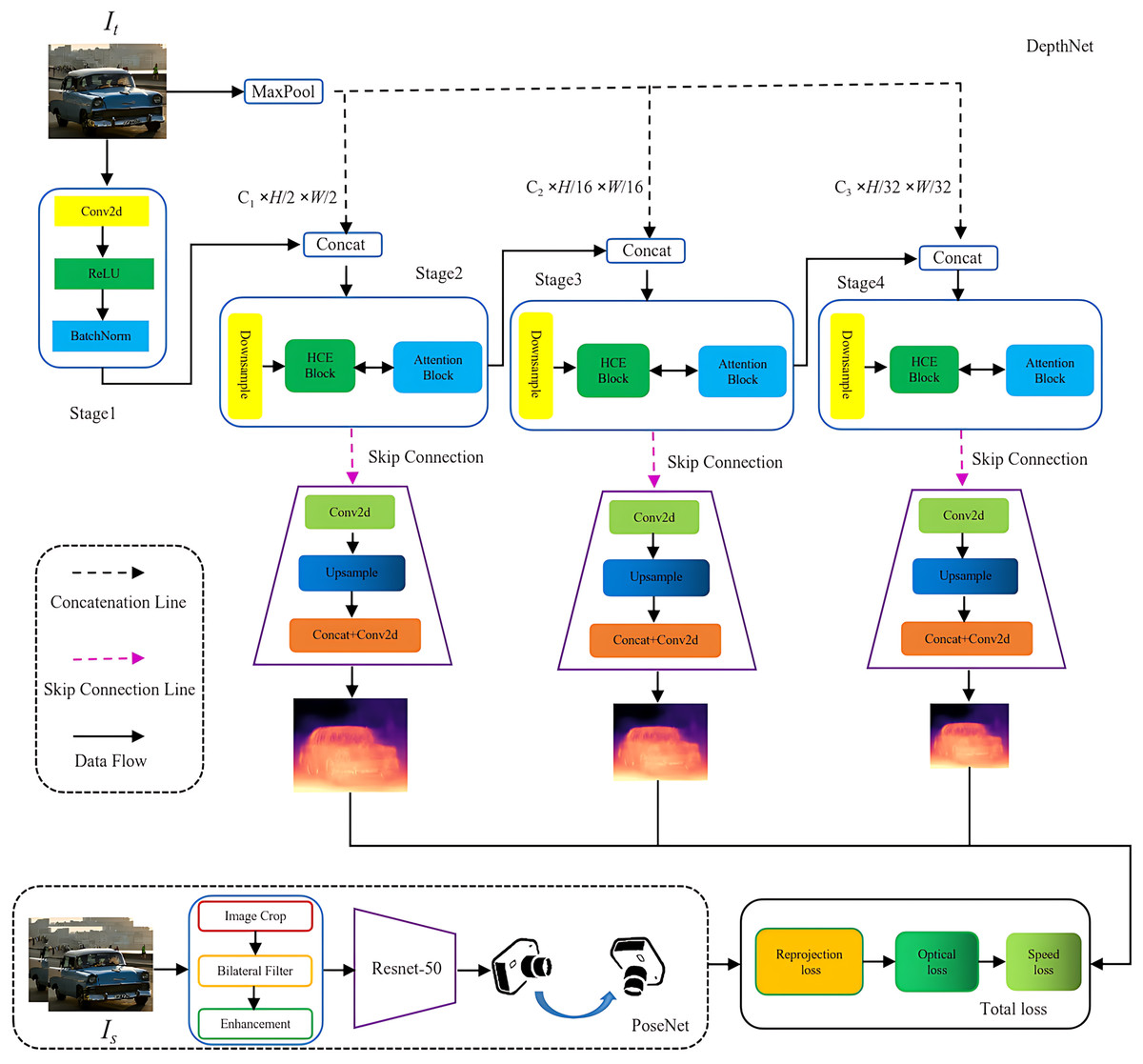
Figure 3: Overview of the proposed DeepFusion network.
The proposed DeepFusion Network primarily comprises DepthNet and PoseNet, along with a comprehensive loss function. DepthNet is organized into four stages that include both encoding and decoding processes. Before the concatenation of each layer, a max pooling operation is performed. Following downsampling, the HCE module and attention block operations are applied prior to employing skip connections. This sequence is succeeded by convolutional layers, upsampling, and additional convolutions to generate depth estimation features. PoseNet shares the Resnet50 architecture with DepthNet; although it may demonstrate slightly slower training speeds, it excels in capturing intricate image detail features. The loss function integrates reprojection loss, optical flow loss, and speed loss.
The proposed network architecture incorporates Hierarchical Context Encoding through initial layers consisting of Conv2D, BatchNorm, ReLU, and MaxPool. This is followed by residual blocks that facilitate the extraction of multiscale features. The encoded features undergo further processing via four context processing modules with varying dilation rates, specifically designed to enhance multiscale contextual representation. This integrated design ensures robust depth estimation while improving precision and enabling fine-grained detail recovery.
The operations ‘conv1’, ‘bn1’, ‘relu’ and ‘maxpool’ collectively form the initial convolution block of the network, responsible for extracting low-level features from the input images, such as edges and textures (Liu, Wan & Gao, 2024; Panda et al., 2022; Ming et al., 2021; Targ, Almeida & Lyman, 2016). Given an input image , the initial convolution block applies a transformation where:
(10)
Here, and denote the reduced spatial dimensions after downsampling and are the depth of the output feature. This transformation aids in preserving critical feature details by minimizing spatial redundancy, thereby facilitating efficient feature extraction for subsequent layers. These layers progressively increase the number of channels in the feature maps (width) while simultaneously reducing the spatial dimensions, ultimately forming high-level semantic features. In layer 4, a multigrid mechanism and dilated convolutions are employed to expand the receptive field, enabling the network to capture broader contextual information from a larger area.
Hierarchical context encoding module
Unlike traditional methods that utilize context encoding in image segmentation, we incorporate multiscale HCE modules into the depth estimation pipeline. This integration enables the network to more effectively address depth discontinuities and large-scale variations in depth (Zhang et al., 2018; Nguyen, Fookes & Sridharan, 2020; Chen et al., 2018). The HCE module extracts hierarchical features through multiscale convolutions. By expanding the receptive field, it captures contextual information across multiple scales, thereby facilitating accurate depth estimation for objects situated at varying distances. In conventional convolutional operations, the growth of the receptive field is gradual as the kernel size increases. However, with hierarchical context encoding, we can enhance the receptive field without augmenting the number of parameters. The convolution operation is defined as follows:
(11) Regarding Eq. (11), is the input feature map, is the convolution filter, is the multi-scale factor, is the output feature map, is the spatial index in the input feature map. When set the different multi-scale factor , the convolution kernel operates at multiple spatial scales, allowing it to aggregate information from a broader context while preserving both the number of parameters and feature map resolution. This is crucial for capturing context at different scales without pooling layers, which typically reduces resolution.
HCE employs multiscale feature extraction with a multi-scale factor D set to 1, 3, 6, and 12. A global feature aggregation layer integrates global scene context and subsequently feeds this information into the decoder for dynamic geometry-aware decoding. This process refines geometric details and enhances boundary precision, resulting in the generation of four inverse depth maps at multiple scales. Additionally, we utilize an optical flow decoder to estimate dense motion fields, incorporating dynamic constraints that significantly improve depth estimation accuracy. This architecture effectively combines multiscale context, global scene understanding, and motion-guided constraints to achieve precise and robust depth estimation.
The module applies several parallel convolutions with different multi-scale factor, and then concatenates the results. The formula for HCE’s output is as follows:
(12)
Regarding Eq. (12),
is the result of a convolution (captures local information).
, , are the results of convolutions with multi-scale factor of 6, 12, and 18, respectively.
is the output of the global average pooling, which captures the global context by aggregating the features throughout the image.
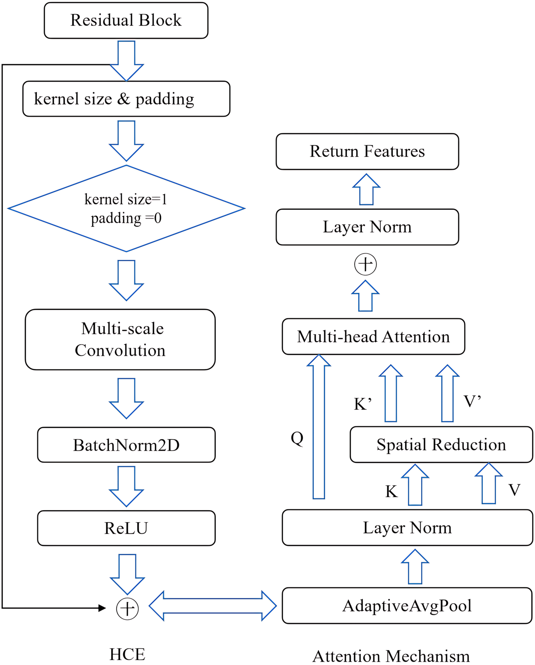
Figure 4 illustrates the hierarchical context encoding and attention mechanism. Each branch of the HCE module is designed to capture features at varying scales, thereby enhancing the network’s ability to effectively manage objects of different sizes in a single pass. This capability addresses a significant challenge in monocular depth estimation.
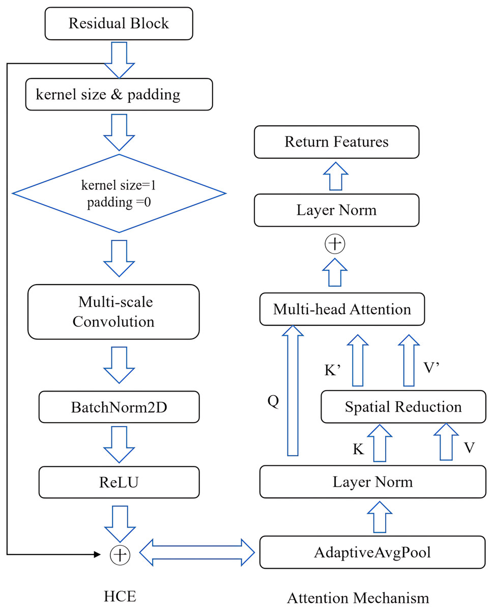
Figure 4: Hierarchical context encoding and attention mechanism.
Multi-scale feature fusion and enhancement
In the context of monocular depth estimation, extracting features at multiple scales is crucial to capture both fine details and global structures of the scene. However, simply extracting features at different scales may not be sufficient for complex scenarios. Thus, it is important to enhance and fuse these multiscale features to ensure that the model can effectively utilize the information at different levels. To enhance the features extracted by the encoder, hierarchical context encoding modules are employed in the feature extraction process (Jie, Yian & Bin, 2024). The modules are designed to capture context at multiple scales by employing convolutional operations with varying receptive field sizes, allowing the network to focus on both local details and broader contextual information. This ensures that the model can better handle varying depth ranges within a single scene.
Figure 5 presents a comparison of different processing stages through three images. The first image represents the original input, devoid of any processing; the second image overlays the feature map extracted using the standard ResNet feature extraction algorithm, which illustrates the fundamental structural features of the image. The third image incorporates a feature map enhanced by the hierarchical context encoding algorithm, emphasizing intricate details and complex patterns within the image. This demonstrates the advantages of this approach in enhancing feature representation.
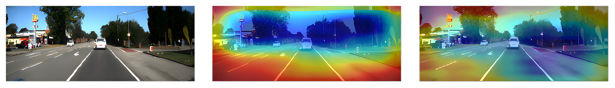
Figure 5: Multi-Scale Feature Enhancement.
(A) The original image data. (B) The image overlays the feature map extracted using the standard ResNet feature extraction algorithm, which illustrates the fundamental structural features of the image. (C) The image integrates a feature map that has been enhanced through our hierarchical context encoding algorithm, highlighting intricate details and complex patterns present within the image.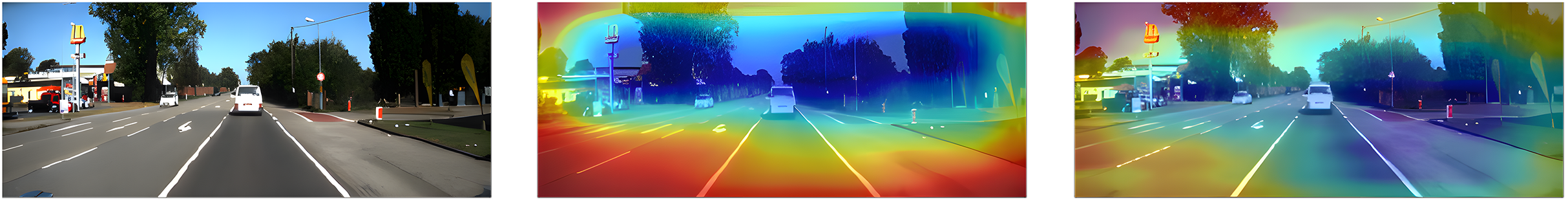
Feature attention module
The feature attention module is employed on the combined feature maps generated by the HCE module. This module integrates both spatial and channel-wise attention mechanisms, which selectively enhance the most pertinent regions of the feature map, such as edges and object boundaries, while attenuating less informative areas. By introducing a spatial attention mask and a channel-wise attention mask , this module improves the focus on critical regions.
The enhanced feature map is computed as:
(13) where denotes multiplication by element. The spatial mask is computed as:
(14)
The channel mask is derived by combining the global averages.
(15) With representing the sigmoid function. This formulation strengthens the ability of the model to emphasize essential features, ultimately improving the network’s performance in depth estimation.
Double frame coupled reprojection
The loss function facilitates the depth network and the pose network in predicting values that minimize re-projection error, thereby refining both depth estimation and camera pose prediction. In contrast to other methods (Godard et al., 2019; Guizilini et al., 2020), which utilize a minimum reprojection error approach based on four consecutive frames for projection, our method introduces an enhancement by employing only two frames. This not only improves efficiency but also maintains or even surpasses state-of-the-art performance. Furthermore, we propose a bidirectional re-projection loss function that computes re-projection errors in both temporal directions. This bidirectional perspective allows the network to effectively capture scene geometry from both views, mitigating the effects of occlusions and significantly enhancing generalization capabilities. In comparison, previous works have predominantly relied on unidirectional re-projection methods, which restrict the network’s ability to learn comprehensive representations of scenes.
From frame to frame (‘pred_0_from_1’), this corresponds to projecting the first frame into the reference frame and computing the reprojection loss.
From frame to frame (‘pred_1_from_0’), this corresponds to projecting the reference frame into the first frame and computing the reprojection loss.
For each pixel in frame 0, the corresponding position in frame 1 is determined by the predicted depth and camera pose. The reprojection loss is calculated by warping the image according to this geometric mapping and comparing the warped image with the original, thereby assessing the accuracy of the predictions. Specifically:
(16) is the intensity of the pixels in position in the target frame. is the intensity of the pixels in the position in the source frame, warped according to the flow field. is the location in the source frame obtained by applying the flow field.
The loss function is computed for both the forward flow (warping frame 1 to frame 0) and the backward flow (warping frame 0 to frame 1). The objective is to minimize the difference between the original and warped frames. For the forward flow:
(17)
For the backward flow:
(18)
Flow consistency ensures that the forward and backward flow fields are mutually consistent. This means that if a pixel in frame 0 is moved to frame 1 by the forward flow, the backward flow should return the pixel to its original location in frame 0. The flow consistency loss can be written as
(19) where is the location in frame 1 that corresponds to frame 0, according to the forward flow. This term penalizes inconsistencies between the forward and backward flow fields, encouraging the network to predict a more accurate and consistent flow.
The total flow loss combines the forward and backward re-projection losses with the flow consistency loss:
(20) In Eq. (20), is the forward reprojection loss, is the loss of reverse reprojection, is the loss of consistency, is a weighting factor (in the current code, it is set to 0.1) that balances the importance of flow consistency relative to the reprojection error.
Double frame coupled reprojection involves the transformation from timestamp t to t + 1, represented by frames 0 and 1 respectively, which corresponds to the pose transformations and . By computing the reprojection loss in both directions, this approach enhances the robustness of depth estimation against bidirectional transformations. Such a strategy improves the model’s generalization capabilities by considering both forward and backward reprojections, representing a significant advancement over methods that rely solely on single-direction reprojection.
Speed fusion for absolute depth estimation
In monocular depth estimation, a significant challenge is the scale ambiguity problem. This issue arises because the network can estimate relative depth but lacks the capability to predict metric depth (Wang et al., 2024; Zhang, Song & Lou, 2024; Bian et al., 2019; Liu et al., 2015; Johnston & Carneiro, 2020; Gordon et al., 2019). We addressed this challenge through speed supervision, leveraging speed measurements obtained from the inertial measurement unit (IMU) to inform the predicted depth. However, since speed derived from the IMU results from integrating acceleration data, it tends to drift over time, leading to inaccuracies in both speed and angle estimations. Our proposed speed supervision technique integrates IMU data with information regarding the vehicle’s own speed. This approach not only ensures that the predicted depth maps maintain metric consistency across different sequences but also enhances the accuracy of absolute depth estimation.
Given a vehicle’s ground truth speed , the network estimates the depth by predicting the relative motion between frames. The speed can be inferred from the predicted depth and pose as
(21) where:
is the distance traveled by the vehicle, calculated from the translation vector (the pose predicted by the network).
is the time interval between frames (typically known from the timestamps).
(22) Here, represents the translation vector between the two frames.
Speed loss function
This speed loss function is designed to supervise the depth estimation process by comparing the model’s predicted motion between frames with the actual motion derived from the fusion of IMU data and vehicle speed. The IMU captures both linear acceleration and angular velocity, while the vehicle controller provides information on vehicle speed and front wheel steering angle via the CAN bus. Our innovative approach facilitates a more accurate estimation of the vehicle’s displacement through effective data fusion. The primary objective is to enforce consistency between the model’s predicted translation (displacement) and the actual measured speed, thereby ensuring that the predicted depth is appropriately scaled in metric units.
We propose a novel loss function that leverages both linear acceleration and angular velocity obtained from the IMU, in conjunction with vehicle speed, to compute an absolute scale for depth estimation.
-
1.
IMU data integration
Given linear acceleration and angular velocity over a time interval : (23) (24) (25)
-
2.
Integration of vehicle speed and steering angle
Given the vehicle speed and steering angle : (26) (27)
-
3.
Data synchronization and fusion (28) (29) where is the fusion weight.
-
4.
Displacement and rotation fusion (30)
(31) We introduce a novel loss function that is grounded in the displacement and rotation of the fused components. Specifically, this loss function penalizes the discrepancy between the predicted translation and the fusion translation over a specified time interval: (32) (33) (34) (35) (36) The formula is the predicting displacement, which serves as a scale factor. The overall fusion spatial displacement is composed of the translational velocity spatial displacement and the rotational velocity spatial displacement, where represents the weight for rotation displacement.
-
6.
Final loss function
The final speed loss is computed as an average across all frames. The purpose of this loss function is to ensure that the model’s predictions regarding the relative pose between frames—specifically in terms of translation—are consistent with the speed measurements obtained from the IMU, which serves as a ground truth for real-world motion. The overall speed loss can be expressed as follows: The final loss function is averaged over all frames. (37) (38) (39) The multiplication by accounts for the specific time interval between frames, thereby ensuring consistency in speed units. This loss function encourages the depth estimation network to achieve a more accurate scale in its depth predictions by aligning the model’s predicted motion with real-world motion as measured through IMU and vehicle speed fusion. Consequently, this enables the model to perform inference accurately in both static and dynamic scenes.
UMAD dataset
In order to enhance the validation of our algorithm, we not only utilized the KITTI dataset but also constructed a UMAD dataset aimed at improving the accuracy and generalization capabilities of our model. The hardware components employed in this study include FMCW LiDAR, a monocular camera, and an IMU sensor.
The advantages of our LiDAR system compared to the KITTI LiDAR are threefold: (1) The 120-line LiDAR offers greater line density and higher accuracy than the KITTI’s 64-line configuration, achieving a horizontal resolution of 0.1 degrees and a vertical resolution of 0.08 degrees; (2) FMCW LiDAR is capable of obtaining velocity values for each point on dynamic objects, thereby providing valuable insights into how these dynamic entities may influence estimation results in monocular depth estimation—this feature distinguishes it from other datasets such as KITTI, CityScapes, and nuScenes; (3) It can measure both the relative velocity of dynamic objects with respect to the LiDAR itself as well as their absolute velocity relative to the ground.
Monocular camera parameters: The camera is a high-definition monocular camera with a frame rate of 25 Hz and an image length and width of 640 480. Intrinsic parameter of the camera, = 703.64, = 724.82, = 322.55, = 117.60. Extrinsic parameter from LiDAR to camera, = 0.0, = 0.0, = 0.080000. To reduce calibration errors, the camera is installed on top of the LiDAR and concentric with the LiDAR
IMU parameters: The system employs a high-precision 6-degree-of-freedom IMU sensor, which facilitates real-time and accurate acquisition of vehicle pose. This sensor is installed on the upper part of the LiDAR and is positioned 50 mm along the X-axis from the center point of the LiDAR. The IMU sensor plays a crucial role in LiDAR calibration and data synchronization. While it can also provide integral speed information, its accuracy is inferior to that obtained from the vehicle’s CAN port.
The UMAD dataset distinguishes itself from other datasets such as KITTI, CityScapes (Cordts et al., 2016), and nuScenes (Caesar et al., 2020) by utilizing FMCW LiDAR technology (Kim, Jung & Lee, 2020; Wu et al., 2024; Gu et al., 2022). This advanced technology not only captures point cloud data but also delivers velocity information for each individual point. The dataset is available in ROS bag file format and includes a dedicated topic for dynamic points, rendering it highly valuable for research in autonomous driving, robotics, and computer vision. As illustrated in Fig. 6, this integrated sensor system is mounted on the vehicle.
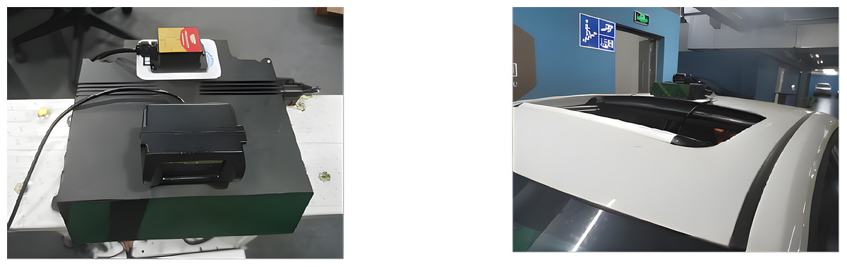
Figure 6: UMAD sensors.
(A) The integrated sensor system employed for the collection of the UMAD dataset consists of a monocular camera, FMCW LiDAR, and an IMU sensor. The point cloud data acquired by the LiDAR is utilized to validate the accuracy of monocular depth estimation through comparative analysis. (B) This integrated sensor system is mounted on the roof of the vehicle. This configuration enables stable, real-world data acquisition across diverse driving environments while maintaining sensor rigidity and calibration consistency.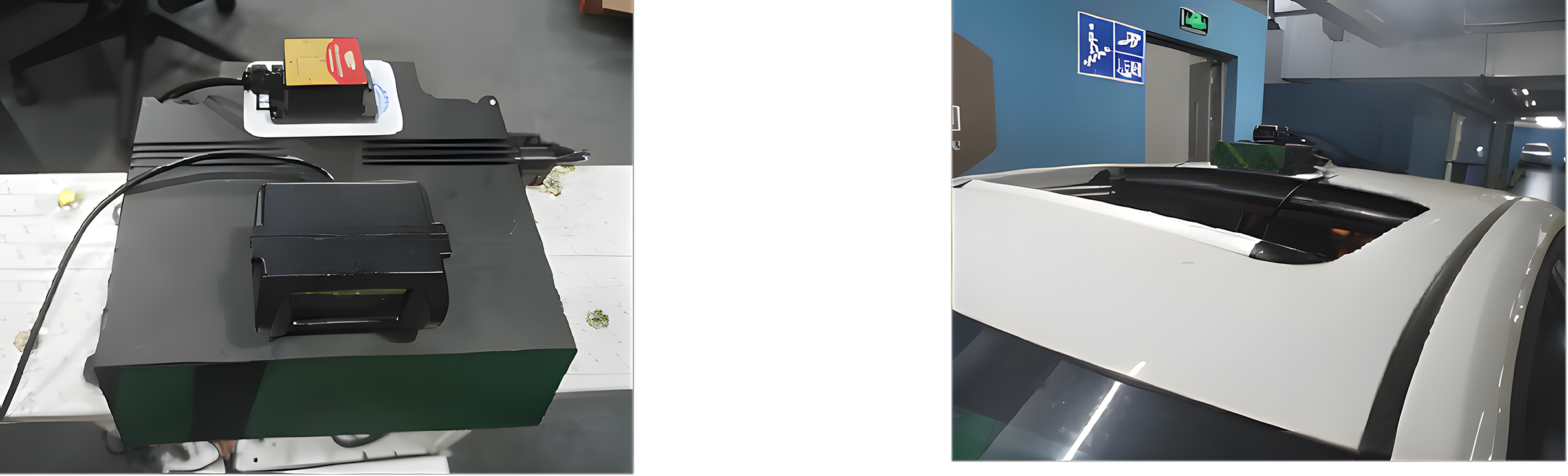
The UMAD dataset comprises approximately 200 GB of data, organized into five distinct scenarios: urban roads, enclosed parks, underground garages, commercial district roads, and night scenes, as illustrated in Fig. 7. Each scenario has a duration of about 10 min. In the figure, the rows from top to bottom correspond to urban roads, enclosed parks, and underground garages respectively. The columns from left to right display the image data alongside the corresponding 3D point cloud data.
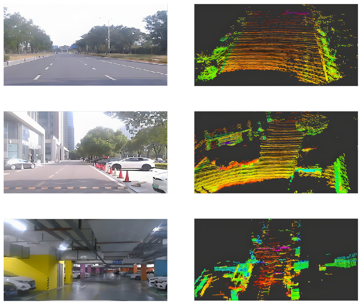
Figure 7: UMAD dataset.
(A) Representative RGB image from the urban roads scenario of the UMAD dataset. (B) Paired point cloud sample corresponding to the urban-road scene in (A). (C) Representative RGB image from the enclosed parks scenario of the UMAD dataset. (D) Paired point cloud sample corresponding to the enclosed-park scene in (C). (E) Representative RGB image from the underground garages scenario of the UMAD dataset. (F) Paired point cloud sample corresponding to the underground-garage scene in (E).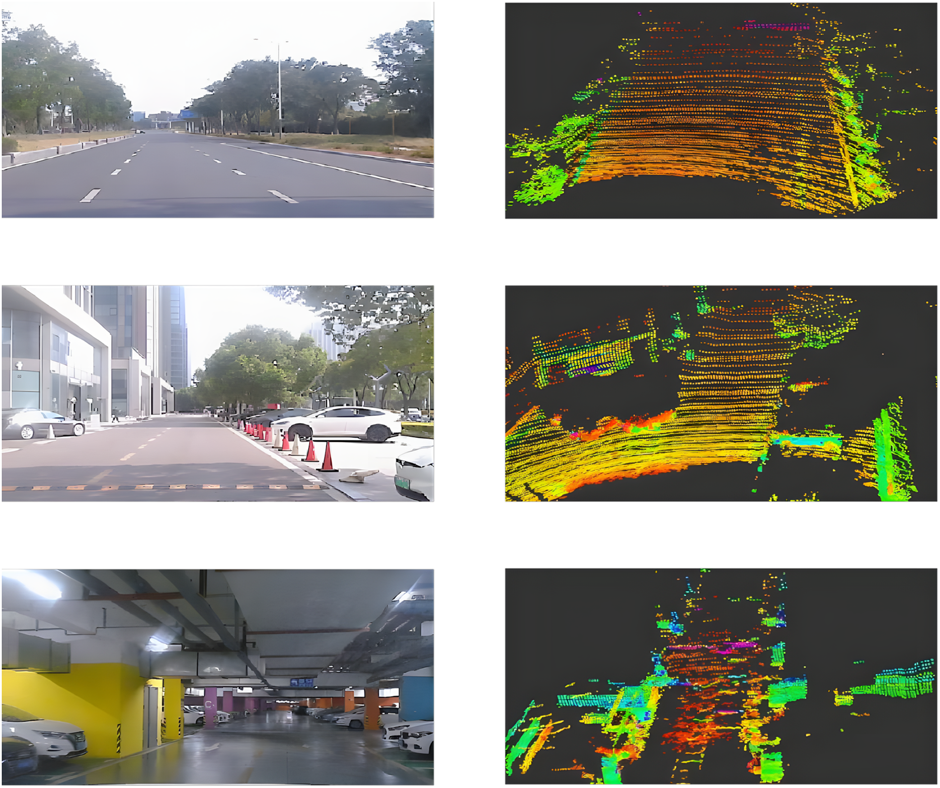
Experiments
The experimental section provides a detailed account of the hardware platform utilized, as well as the composition of both the training and testing datasets. The experimental procedure encompasses image preprocessing, model training, inference, and a comprehensive evaluation. Both qualitative and quantitative analyses are conducted, in addition to an assessment of speed (inference time) and practical applicability, to thoroughly assess the performance of the model.
Datasets
The models were developed and trained using a robust dataset comprising 79,620 images, which were subsequently evaluated on an additional set of 8,848 images. This extensive dataset was meticulously curated to encompass diverse scenes and lighting conditions, thereby ensuring that the model learns from a wide range of depth estimation scenarios. The training and evaluation images are high resolution, measuring 640 192 pixels, and were captured using a monocular camera system with intrinsic parameters normalized to the image size: specifically ( = 0.58), ( = 1.92), and principal point offsets ( = 0.5), ( = 0.5). The preparation of the dataset involved generating ground truth depth maps utilizing LiDAR data from the KITTI dataset, employing sensors to ensure accurate depth supervision. The models underwent fine-tuning on the KITTI raw dataset, where both left- and right-camera images were utilized to reflect the stereo setup. For ground truth depth map generation, LiDAR data were processed with a specific calibration matrix and resized to maintain consistency in training and evaluation. In addition to conducting training evaluations on the KITTI dataset, we also employed the UMAD dataset—which includes FMCW LiDAR data alongside inputs from a monocular camera and an IMU sensor—to enhance both model accuracy and ablation studies.
Implementation details
The hardware configuration utilized in our experiments comprises an Intel® Xeon(R) CPU E5-2680 v4 operating at 2.40 GHz across 28 cores, accompanied by 64 GB of RAM, a 2TB SSD, and an RTX 4060 Ti GPU with 16 GB of memory. The depth estimation component of our project is implemented using the PyTorch framework. Depth maps are computed on the GPU under the following experimental parameters: input images are resized to a height of 192 pixels and a width of 640 pixels. The network architecture is based on the DeepFusion Network and has been trained on the KITTI and UMAD dataset. The training process employs a batch size of 12 and a learning rate set to 1e−4, conducted over a total of 20 epochs. A disparity smoothness weight of 1e−3 was applied, with depth predictions normalized within a range from 0.1 to 90 m. The model initialization incorporates pre-trained weights, while pose estimation is executed through a separate decoder. Training encompasses various loss functions including re-projection loss, smoothness loss, optical flow loss, affine invariant loss, and velocity loss derived from IMU and vehicle fusion data. Our framework also facilitates multiscale training with scales configured as [0, 1, 2, 3]. These parameters were meticulously selected to optimize performance for the specified hardware setup; all computations are efficiently executed on the GPU. Notably, the entire training process requires approximately 10 12 h when conducted on a single NVIDIA RTX 4060 Ti GPU.
We evaluated the performance of our self-supervised monocular depth estimation approach through both quantitative and qualitative comparisons with state-of-the-art methods across various scenes (Liu, Salzmann & He, 2014; Eigen, Puhrsch & Fergus, 2014). For the quantitative assessment, we employed multiple metrics that are commonly utilized in prior research. Performance of the model using standard metrics Abs Rel, Sqr Rel, RMSE, RMSE (log) and , and , respectively, as follows:
Abs Rel: The mean absolute relative error, calculated as
Sqr Rel: The mean squared relative error, defined as
RMSE: The linear root mean square error,
RMSE(log): The logarithmic root mean square error,
Threshold: The percentage of pixels where indicates the fraction within the defined error threshold.
Here, represents the predicted depth for each pixel , and N denotes the total pixel count. We trained the monocular depth network using outdoor scenes, thereby aligning our methodology with recent state-of-the-art approaches. While indoor datasets were excluded from this study, it is important to note that similar training can also be conducted utilizing indoor data.
Depth estimation performance
To systematically evaluate the performance of deep estimation algorithms, we employ a combined approach that integrates qualitative visual comparisons with quantitative metric calculations to comprehensively validate the predictive accuracy of the models.
Figure 8 presents a qualitative comparison of monocular depth estimation performance, showcasing DeepFusion alongside previous methodologies using frames from the KITTI dataset (Eigen test split). Our approach exhibits an improved capacity to capture finer details and structures—such as those present in vehicles, pedestrians, and slender poles—attributable to its multi-scale learned preservation of spatial information. Our models were trained for 20 epochs at a resolution of 640 × 192 with a batch size of 12. In contrast, SfMLearner (Godard, Mac Aodha & Brostow, 2017) underwent training for 200 epochs at a resolution of 416 × 128 with a batch size of 4. For Lite-Mono (Zhang et al., 2023), training was performed over the course of 30 epochs at a resolution of 640 × 192 utilizing the same batch size of 12. Similarly, Monodepth2 (Godard et al., 2019) was trained for 20 epochs at a resolution of 640 × 192 while employing an identical batch size of 12.
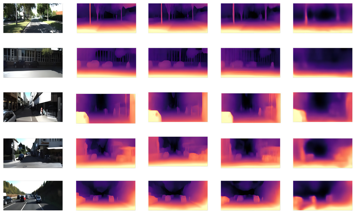
Figure 8: Qualitative comparison result.
(A) Original RGB input image. (B) Depth map predicted by our DeepFusion model. The result demonstrates superior depth accuracy, particularly for dynamic vehicles and small, stationary objects. (C) Depth map estimated by the Lite-Mono model. (D) Depth map estimated by the Monodepth2 model. (E) Depth map estimated by the SfMLearner model.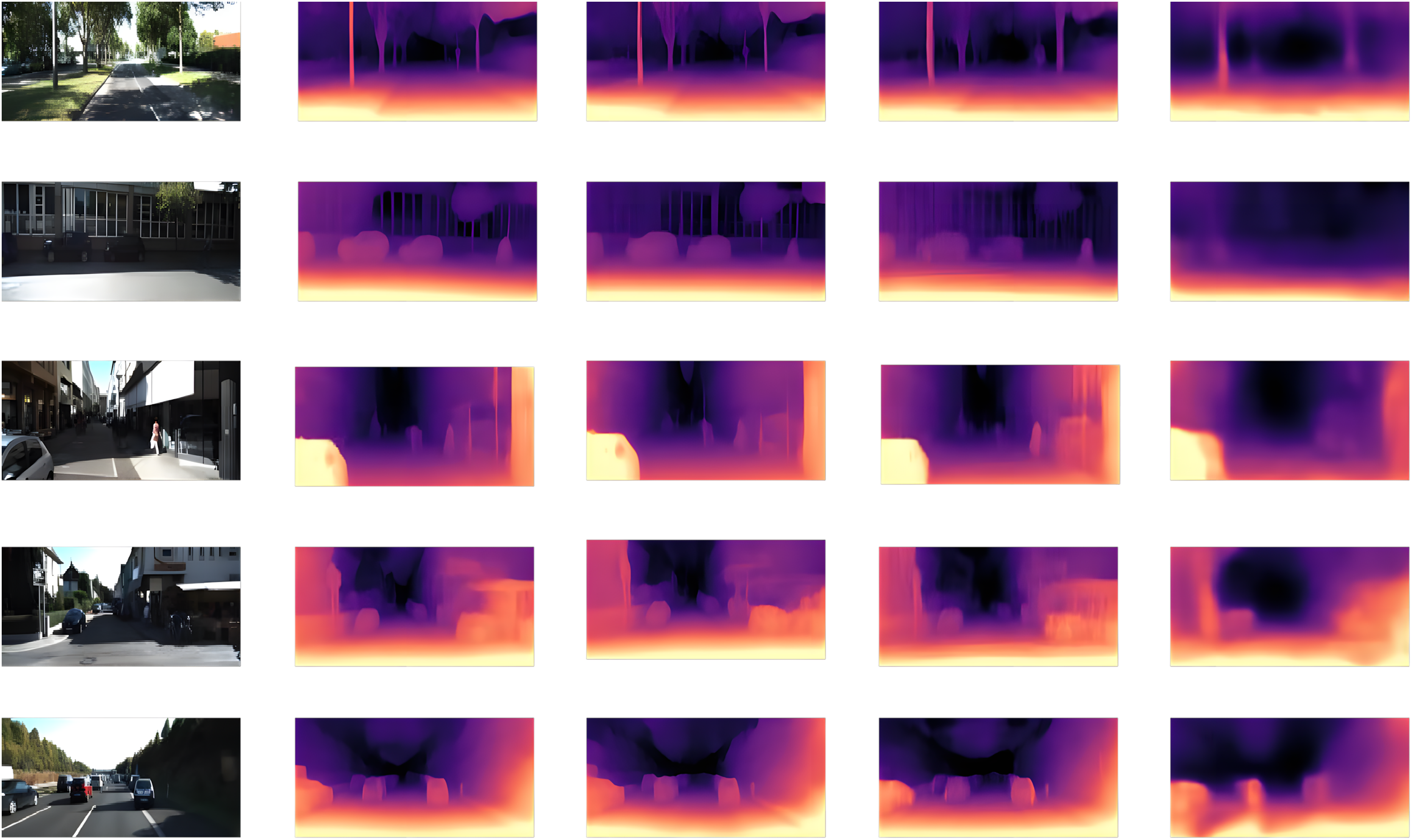
The depth estimation process employs a multiscale decoder along with a dynamic scale factor to produce accurate and scale-consistent depth maps from monocular images. As illustrated in Fig. 9, (a) represents the original image, (b) depicts the disparity map, and (c) shows the disparity map converted into a point cloud. In contrast to previous self-supervised monocular depth estimation methods (Godard et al., 2019; Chen et al., 2016; Zhou et al., 2017; Zhang, Zhang & Tao, 2022), our model broadens the scope of depth estimation to encompass both outdoor and indoor environments. The images were captured in a spontaneous manner across diverse environments, including libraries, offices, factory interiors, and airport terminals.
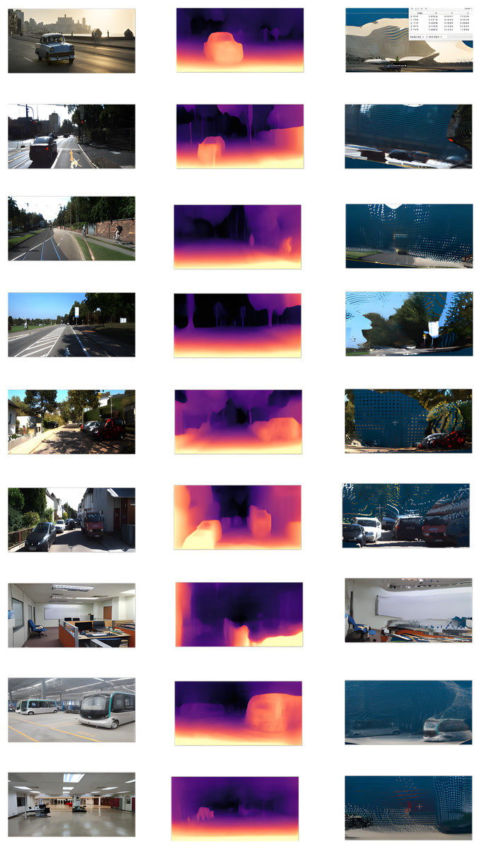
Figure 9: Qualitative assessment across various scenarios.
(A) Original RGB images collected in a variety of real-world environments, such as libraries, offices, factory interiors, and airport terminals. (B) Disparity maps predicted by our algorithm, illustrating its ability to recover fine-grained geometric structure from a single image. (C) Points cloud reconstructed from the predicted disparity. The results show that our model extends monocular depth estimation to a broad range of indoor and outdoor scenarios with strong geometric consistency.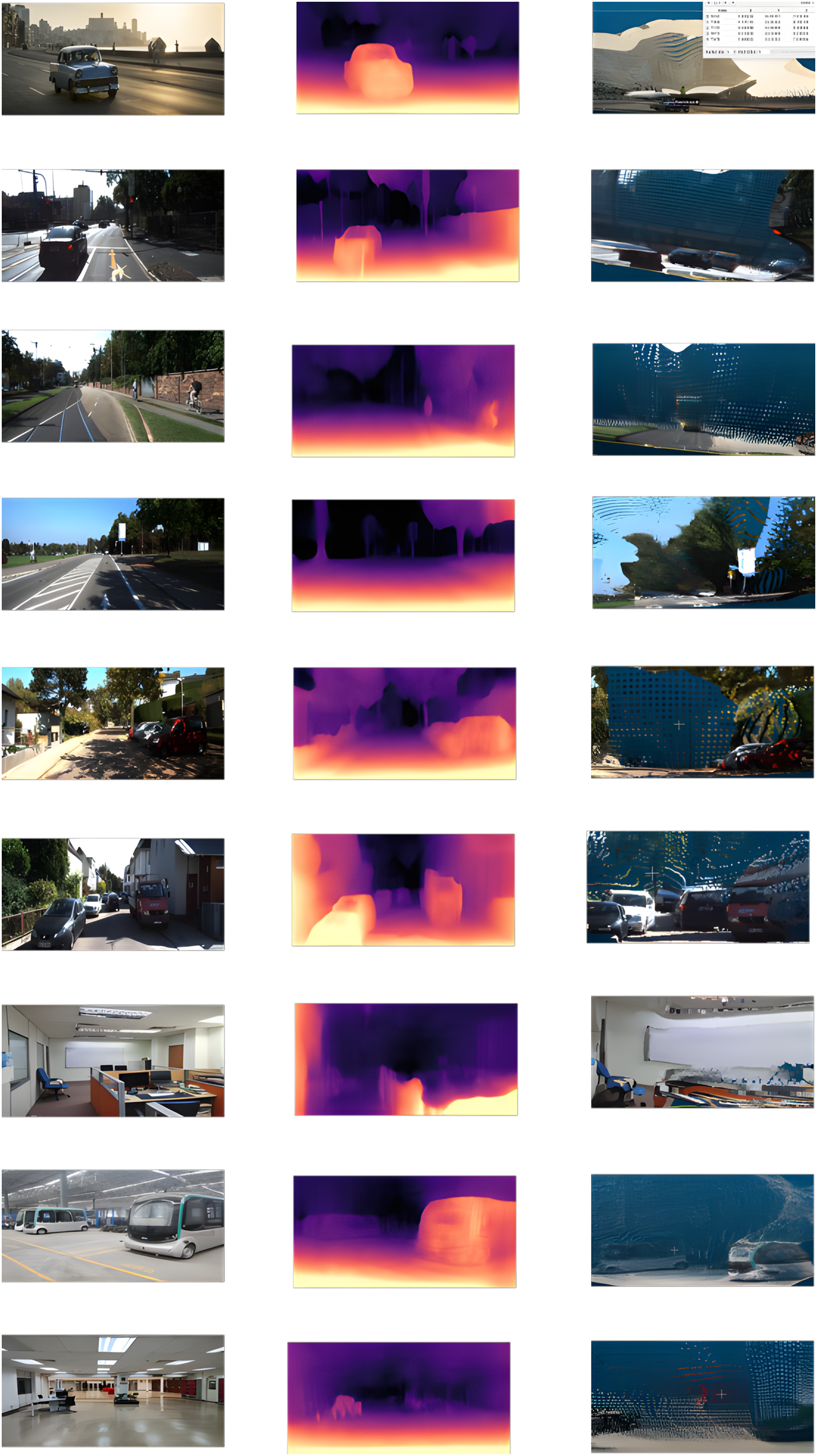
As illustrated in Table 1, DeepFusion demonstrates significantly superior performance. The comparative data are sourced from Monodepth2 (Godard et al., 2019), R-MSFM (Zhou et al., 2021), Lite-Mono (Zhang et al., 2023), and Eite-Mono (Ren, 2024). Depth Error ( ) indicates that a lower value is preferable, while Depth Accuracy ( ) signifies that a higher value is desirable (Shi et al., 2024; Peluso et al., 2020; Ai & Wang, 2024). “M” denotes KITTI monocular videos; “M∗” refers to an input resolution of 1,024 320; and “M ” indicates models trained without pre-training on ImageNet (Deng et al., 2009). The best results are highlighted in bold.
| Method | Data | Depth error ( ) | Depth accuracy ( ) | |||||
|---|---|---|---|---|---|---|---|---|
| Abs Rel | Sq Rel | RMSE | RMSElog | |||||
| Monodepth2-Res18 | M | 0.115 | 0.903 | 4.863 | 0.193 | 0.877 | 0.959 | 0.981 |
| Monodepth2-Res50 | M | 0.110 | 0.831 | 4.642 | 0.187 | 0.883 | 0.962 | 0.982 |
| R-MSFM3 | M | 0.114 | 0.815 | 4.712 | 0.193 | 0.876 | 0.959 | 0.981 |
| R-MSFM6 | M | 0.112 | 0.806 | 4.704 | 0.191 | 0.878 | 0.960 | 0.981 |
| Lite-Mono | M | 0.107 | 0.765 | 4.561 | 0.183 | 0.886 | 0.963 | 0.983 |
| Eite-Mono | M | 0.105 | 0.751 | 4.503 | 0.182 | 0.890 | 0.964 | 0.983 |
| DeepFusion | M | 0.103 | 0.694 | 3.892 | 0.155 | 0.937 | 0.968 | 0.985 |
| Monodepth2-Res18 | 0.132 | 1.044 | 5.142 | 0.210 | 0.845 | 0.948 | 0.977 | |
| Monodepth2-Res50 | 0.131 | 1.023 | 5.064 | 0.206 | 0.849 | 0.951 | 0.979 | |
| R-MSFM3 | 0.128 | 0.965 | 5.019 | 0.207 | 0.853 | 0.951 | 0.977 | |
| R-MSFM6 | 0.126 | 0.944 | 4.987 | 0.204 | 0.857 | 0.952 | 0.978 | |
| Lite-Mono | 0.121 | 0.876 | 4.926 | 0.199 | 0.859 | 0.953 | 0.980 | |
| Eite-Mono | 0.116 | 0.868 | 4.810 | 0.193 | 0.870 | 0.956 | 0.980 | |
| DeepFusion | 0.112 | 0.849 | 4.263 | 0.075 | 0.887 | 0.961 | 0.980 | |
| Monodepth2-Res18 | 0.115 | 0.882 | 4.701 | 0.190 | 0.879 | 0.961 | 0.982 | |
| R-MSFM3 | 0.112 | 0.773 | 4.581 | 0.189 | 0.879 | 0.960 | 0.982 | |
| R-MSFM6 | 0.108 | 0.748 | 4.470 | 0.185 | 0.889 | 0.963 | 0.982 | |
| Lite-Mono | 0.102 | 0.746 | 4.444 | 0.179 | 0.896 | 0.965 | 0.983 | |
| Eite-Mono | 0.101 | 0.731 | 4.365 | 0.177 | 0.899 | 0.965 | 0.983 | |
| DeepFusion | 0.057 | 0.716 | 3.692 | 0.175 | 0.977 | 0.968 | 0.985 | |
Metric depth estimation evaluation
In Fig. 10, the original image data and ground-truth data were sourced from the KITTI dataset, specifically identified as 2011_09_26_drive_0022_sync. The images are numbered sequentially from top to bottom as follows: 26_001_l, 34_215_l, 22_473_r, and 28_497_l. Each row is arranged from left to right, displaying the original image, the point-cloud data derived from the disparity map, and in the final column, the corresponding ground-truth point-cloud data. In this experiment, the speed_loss_weight was set to 0.2 with a total of 10 epochs and a learning rate of 1e−4. Three points were selected in each image; specific coordinate values can be found in Table 2. By comparing these coordinate values, we can assess whether there is consistency between the estimated depth values and their actual counterparts.
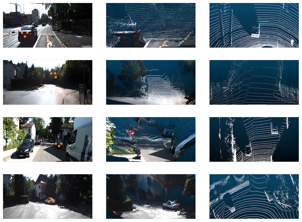
Figure 10: Metric depth accuracy assessment.
(A) Original RGB input images. (B) Points cloud generated by transforming the predicted disparity map. (C) Ground-truth points cloud from the KITTI dataset. In each scene, three spatially distributed points are sampled to compare our reconstructed geometry with the ground truth, providing a reliable evaluation of the accuracy of our depth estimation method.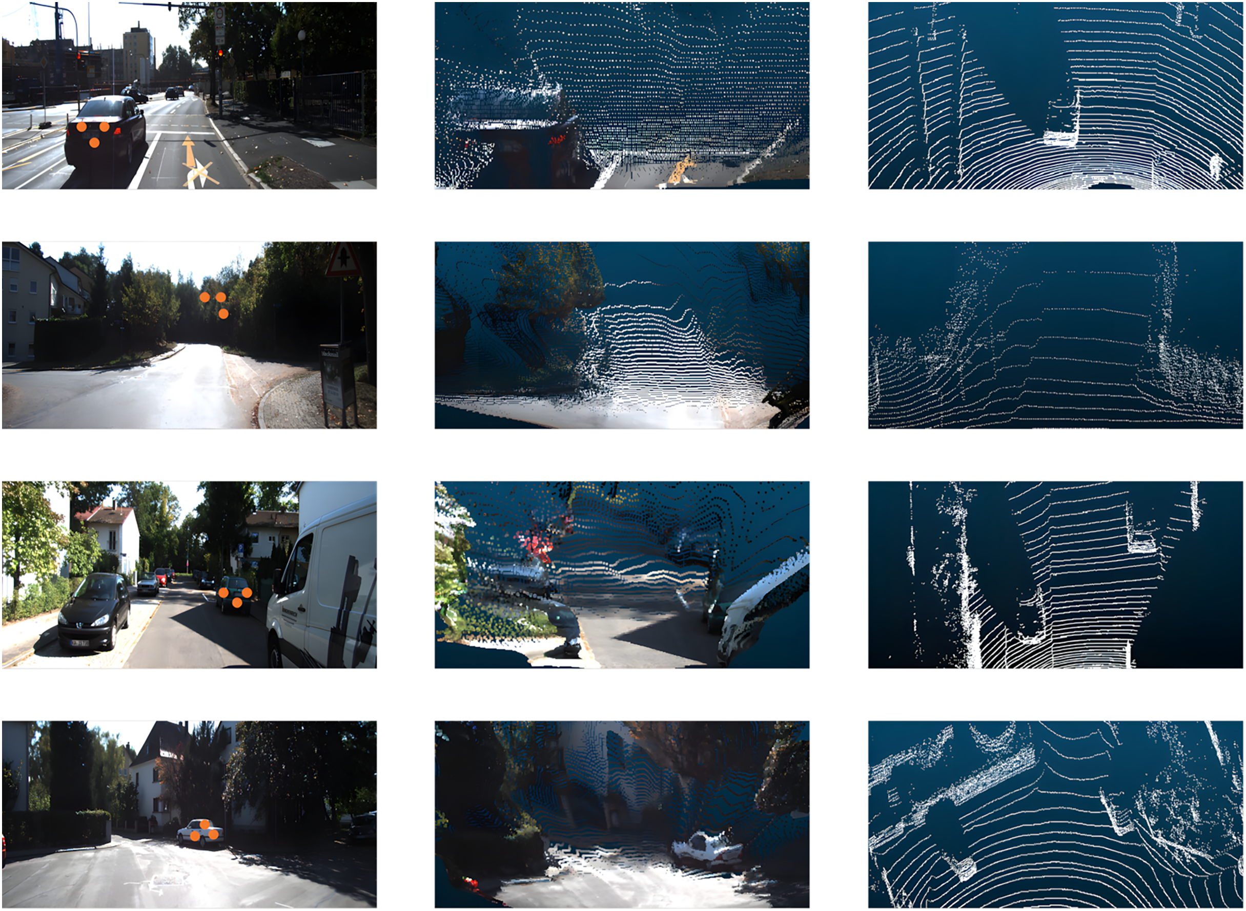
| Coord. | p0 | p0(GT) | p1 | p1(GT) | p2 | p2(GT) |
|---|---|---|---|---|---|---|
| x | −3.698461055 | −3.045000076 | −2.579394102 | −2.407000064 | −3.003914356 | −2.68099994 |
| y | 0.887732148 | 0.829999983 | 0.924798607 | 0.805999994 | 1.214325666 | 1.136000037 |
| z | 7.981794834 | 6.596000194 | 7.253569126 | 6.67299985 | 8.139073371 | 6.579999937 |
| x | 12.789839744 | 13.14254272 | 12.562968254 | 12.10798467 | 12.517499923 | 13.05323640 |
| y | −1.931798696 | −1.558320948 | −2.61036886 | −2.696485376 | −1.859669566 | −1.799743697 |
| z | 79.126472473 | 78.24500326 | 74.021804809 | 74.986057604 | 76.172065734 | 75.257004454 |
| x | −3.712627649 | −2.832999946 | −3.208750247 | 2.52300001 | −3.387167692 | 2.66599889 |
| y | 0.579190254 | 1.080999970 | 0.710117220 | 1.154999971 | 1.141713857 | 1.243999958 |
| z | 6.470081806 | 6.570000171 | 6.544440269 | 6.761000156 | 5.327612876 | 6.54899786 |
| x | 0.982136189 | 1.371000051 | 1.568079113 | 1.83500038 | 1.512231469 | 1.899999976 |
| y | 0.515977382 | 0.814000010 | 0.701763808 | 0.805999994 | 0.740789058 | 0.9969999790 |
| z | 15.850824356 | 17.927999496 | 16.168638229 | 17.756000518 | 15.171360015 | 17.319999694 |
The data presented in Table 2 correspond to Fig. 10, arranged from top to bottom. Three points, denoted as p0, p1, and p2, were selected from the generated depth estimation point cloud map, and their coordinates were recorded. Similarly, three corresponding points—p0(GT), p1(GT), and p2(GT)—were extracted from approximately the same locations within the ground truth point cloud data. Although selection of point positions may not achieve complete precision, the deviation in depth values remains within a margin of 2.0 m. This level of accuracy is deemed sufficient for practical perception applications in specific scenarios. The results indicate that our DeepFusion network effectively mitigates the inherent scale ambiguity associated with monocular systems, ensuring that the generated depth maps are consistent with real-world scales.
To enhance our understanding of the dispersion in depth estimation, we compute the average Euclidean distance, standard deviation, and standard error of the target points.
In Fig. 11, randomly sample depth estimation images from the evaluation dataset and convert them into pseudo-point clouds. Randomly extract point coordinates from the point cloud and compare them with the ground truth point cloud data. Calculate the average Euclidean distance , standard deviation and standard error The unit of the vertical axis is meters.
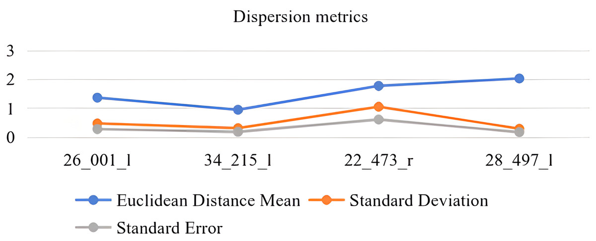
Figure 11: Metric depth estimation.
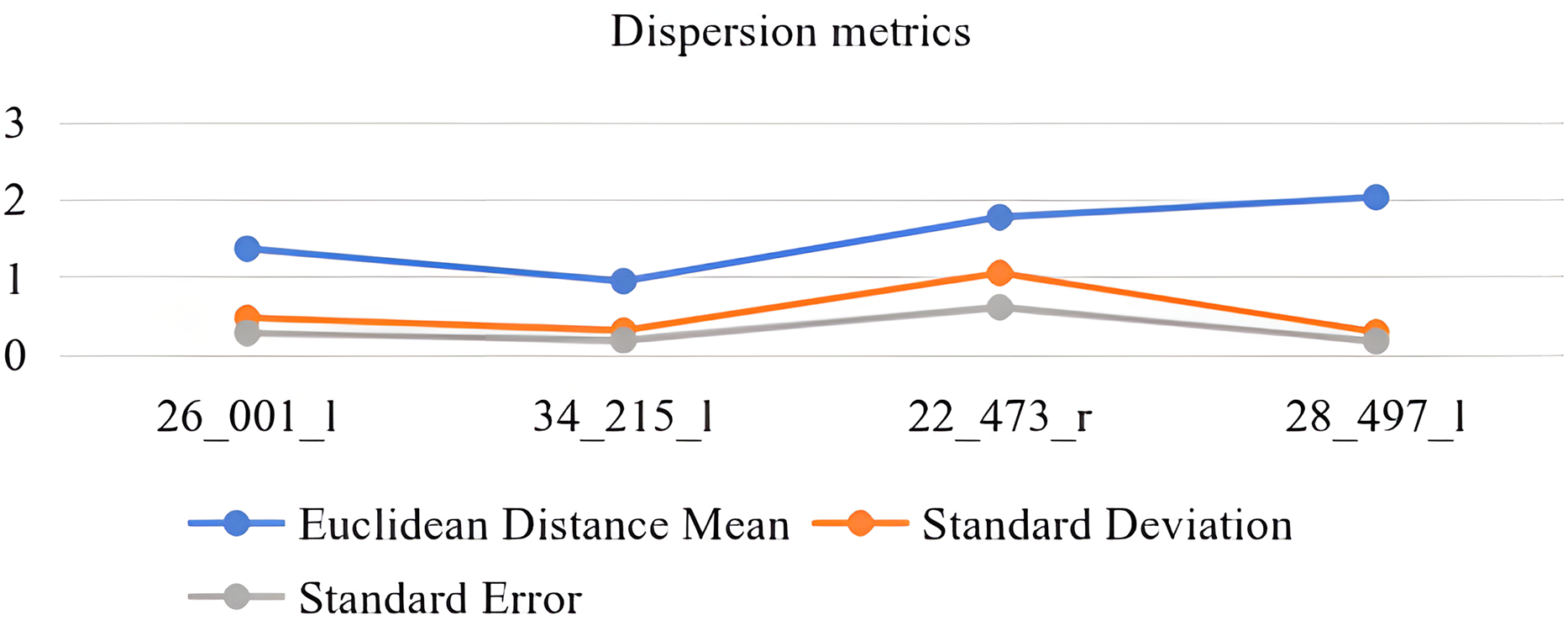
Ablation studies
Table 3 employs checkmarks to signify the adoption of a method, while crosses ✗ indicate that a method is not adopted. The term “training hours” refers to the total duration from the commencement to the conclusion of the training process. Our models were trained for 20 epochs at a resolution of 640 192 with a batch size of 12. The best results are emphasized in bold font.
| HCE | Speed_loss | Flow_loss | Training hours | Abs Rel | Sq Rel | RMSE | RMSElog | |||
|---|---|---|---|---|---|---|---|---|---|---|
| ✗ | ✗ | 12.0 h | 0.392 | 5.767 | 10.612 | 0.464 | 0.449 | 0.721 | 0.857 | |
| ✗ | ✗ | 11.0 h | 0.388 | 5.517 | 10.499 | 0.463 | 0.449 | 0.720 | 0.857 | |
| ✗ | ✗ | 12.5 h | 0.375 | 5.141 | 10.299 | 0.454 | 0.453 | 0.728 | 0.864 | |
| ✗ | 13.0 h | 0.392 | 5.767 | 10.612 | 0.464 | 0.449 | 0.721 | 0.857 | ||
| ✗ | 12 h | 0.348 | 5.463 | 10.408 | 0.459 | 0.453 | 0.726 | 0.860 | ||
| ✗ | 11 h | 0.368 | 4.910 | 10.165 | 0.452 | 0.453 | 0.730 | 0.866 | ||
| 12 h | 0.350 | 4.001 | 9.190 | 0.425 | 0.473 | 0.749 | 0.880 |
Speed evaluation and GPU memory occupation
We conducted experiments to evaluate the memory and inference speed parameters of the proposed model utilizing the KITTI dataset. The model achieves an impressive inference speed of 80 frames per second on videos with a resolution of 640 192, when deployed on an RTX 4060Ti GPU. Utilizing the disparity maps generated by the model, we performed conversions from 2D to 3D point clouds as well as object perception experiments. As demonstrated in Table 4, the results indicate that the model meets the real-time object perception requirements essential for autonomous driving applications. Furthermore, the maximum recorded GPU memory usage is 1,192 MB, which renders it suitable for deployment on standard vehicle-mounted controllers.
| Process | Per frame (ms) |
|---|---|
| Monocular depth estimation | 12.49 |
| Disparity to point cloud | 14.71 |
| Targets perception | 17.27 |
| GPU memory | 1,192 MB |
Practical application
Figure 12 illustrates the application of monocular depth estimation, employing a model trained on the DeepFusion network. Initially, the model generates a disparity map, which is subsequently converted into a point cloud through camera interpolation, thereby facilitating three-dimensional target perception. The findings indicate that DeepFusion is capable of achieving precise metric depth estimation for 3D perception of both static and dynamic objects. This capability effectively addresses the requirements of practical perception applications across a diverse array of scenarios.
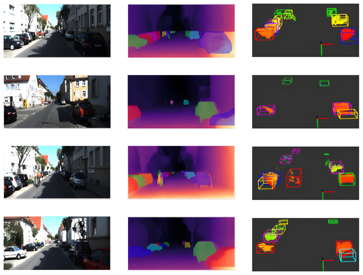
Figure 12: Monocular depth estimation application.
(A) Original RGB images. (B) Fusion target-segmentation disparity maps produced by our framework. (C) The model-predicted disparity maps transformed into a point cloud through camera interpolation, enabling robust 3D target perception. The results demonstrate that DeepFusion achieves precise metric depth estimation for both static and dynamic objects, fulfilling the requirements of real-world perception tasks across a wide range of environments.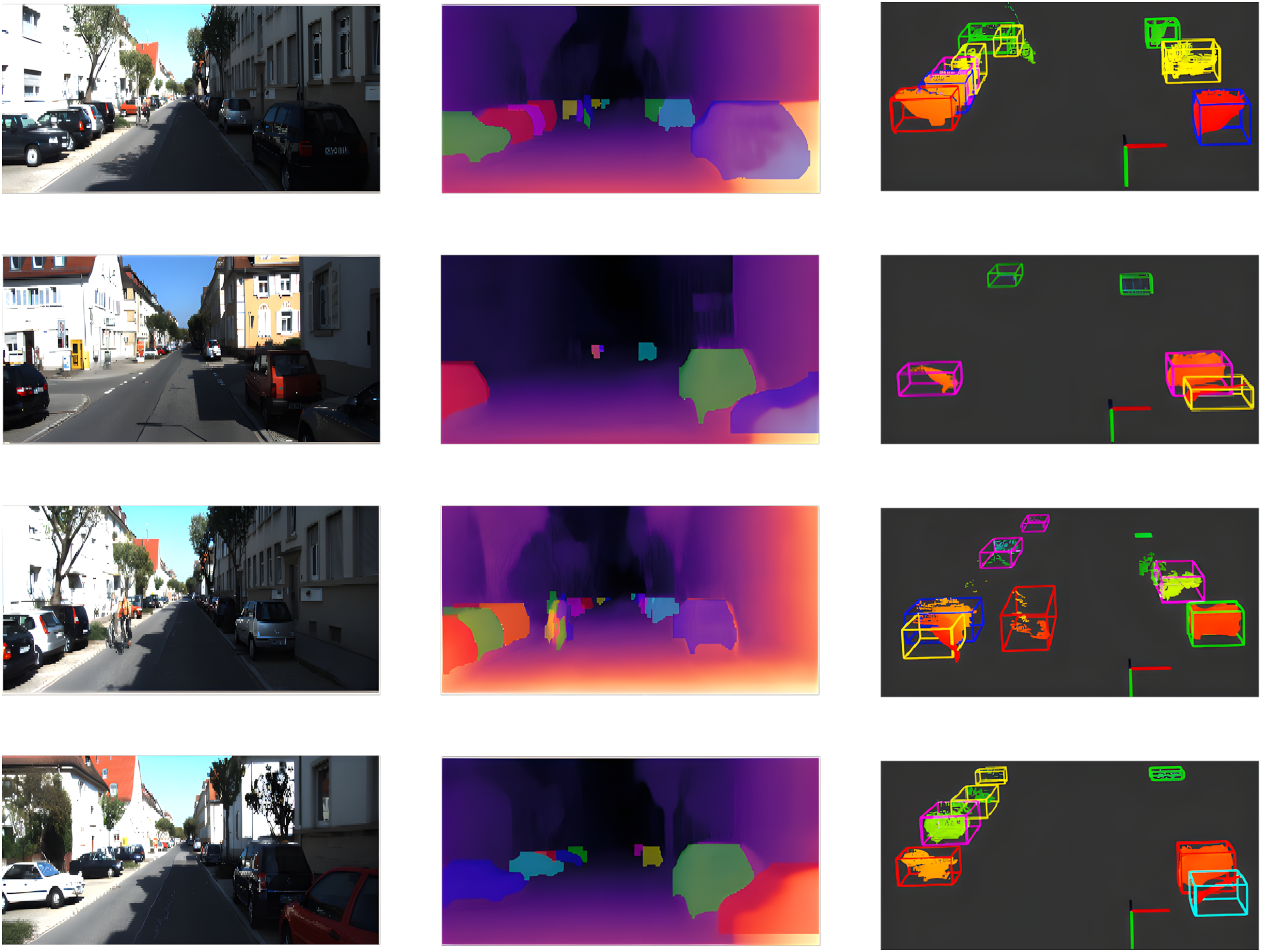
Limitations
Although the depth estimation model presented in this study has demonstrated promising results, several limitations must be acknowledged to further enhance the model’s performance in future work. Firstly, the model’s efficacy may diminish under challenging lighting conditions, such as strong backlighting or intense glare, where accurate depth estimation becomes difficult due to significant variations in illumination. Additionally, the model has not been extensively evaluated in high-speed scenarios, where motion blur could negatively impact its ability to generate reliable depth predictions. These limitations underscore the necessity for further refinement to ensure robust performance across a broader range of real-world conditions. In future research, we intend to address the limitation associated with high-speed scenarios by incorporating the velocity characteristics of FMCW LiDAR point clouds, which will facilitate more accurate training and testing under dynamic high-speed conditions.
Conclusion
In this study, we present a novel monocular depth estimation framework enhanced by several innovations aimed at improving accuracy and robustness.
Our contributions include the development of the DeepFusion network, which incorporates hierarchical context encoding to obtain multi-scale depth fusion features and employs two-frame bidirectional coupling reprojection. This approach refines depth predictions in challenging scenarios involving dynamic scenes or complex geometries while maintaining inference speed.
Additionally, based on a speed total loss function, we introduce kinematic scaling into continuous time frames for gradient backpropagation optimization, significantly addressing the scale ambiguity issue prevalent in monocular depth estimation.
Furthermore, we construct the UMAD dataset—an advanced autonomous driving dataset created using FMCW LiDAR—which serves as the foundational data resource for this research. Alongside this dataset, we develop comprehensive methods for training, testing, and evaluation. These advancements collectively enhance the performance of our framework. Experimental data and practical application results demonstrate the effectiveness of our method, marking it as a significant contribution to monocular autonomous driving perception, robotics, and augmented reality.