
SGCL-DPI: structure-guided curriculum learning for drug-protein interaction prediction
- Published
- Accepted
- Received
- Academic Editor
- Consolato Sergi
- Subject Areas
- Computational Biology, Algorithms and Analysis of Algorithms, Artificial Intelligence, Data Mining and Machine Learning, Neural Networks
- Keywords
- Drug–protein interaction prediction, Curriculum learning, Graph neural networks (GNNs), Random forest knowledge distillation, Similarity graphs, Structure-guided learning, Molecular feature integration, Generalization in bioinformatics, BindingDB and STITCH datasets, Single-modality deep learning
- Copyright
- © 2025 Soufan
- Licence
- This is an open access article distributed under the terms of the Creative Commons Attribution License, which permits unrestricted use, distribution, reproduction and adaptation in any medium and for any purpose provided that it is properly attributed. For attribution, the original author(s), title, publication source (PeerJ Computer Science) and either DOI or URL of the article must be cited.
- Cite this article
- 2025. SGCL-DPI: structure-guided curriculum learning for drug-protein interaction prediction. PeerJ Computer Science 11:e3247 https://doi.org/10.7717/peerj-cs.3247
Abstract
Predicting drug–protein interactions (DPIs) is a critical challenge in bioinformatics and drug discovery, as each computational approach provides only a partial view of these complex molecular relationships. Deep learning techniques such as graph neural networks (GNNs) capture local structural patterns from molecular graphs, whereas classical algorithms like Random Forest (RF) leverage global molecular descriptors. We introduce Structure-Guided Curriculum Learning forDrug-Protein Interaction Prediction (SGCL-DPI), a structure-guided curriculum learning framework that initially leverages the global molecular insights captured by a RF model to guide and progressively refine the structural pattern learning of a GNN, enhancing drug–protein interaction prediction accuracy. SGCL-DPI employs a curriculum learning strategy in which an RF teacher model provides initial high-level predictive guidance to a GNN student model, and the focus of training gradually shifts from the RF to the GNN. The training objective integrates three components: binary cross-entropy for correct interaction classification, knowledge distillation to align the GNN’s outputs with the RF’s predictions, and a structural consistency term to maintain similarity-based relational patterns in the learned representations. We evaluated SGCL-DPI on two benchmark datasets: BindingDB and a challenging STITCH-derived dataset. On the BindingDB dataset, a standalone RF baseline using classical molecular descriptors achieved an area under the receiver operating characteristic curve (AUC-ROC) of 99.18% and an area under the precision–recall curve (AUPR) of 99.14%, outperforming many deep learning models. This result highlights the strong predictive power of traditional descriptors on this dataset. On the more difficult STITCH-derived hard split, SGCL-DPI attained a balanced performance, with an F1-score of 67.06%, an AUC-ROC of 82.33%, and an AUPR of 71.69%. Notably, the model outperformed both a purely GNN-based deep model and the traditional RF baseline in terms of F1-score, demonstrating superior ability to predict interactions for entirely unseen drug–protein pairs. These findings demonstrate that SGCL-DPI effectively bridges classical machine learning and deep learning approaches for DPI prediction. By integrating global descriptor-based knowledge with graph-based structural learning, the proposed framework significantly improves predictive accuracy and generalization on challenging interaction prediction tasks, highlighting a promising direction for future DPI prediction research. The full implementation of the proposed framework is publicly available at https://github.com/soufanom/SGCL-DPI to ensure transparency and reproducibility.
Introduction
Accurately predicting drug-target interactions is a critical challenge in drug discovery and development. Understanding these interactions is pivotal, as they can impact the efficacy, safety, and therapeutic potential of drugs. However, traditional experimental approaches to identifying drug-target interactions are labor-intensive, time-consuming, and costly. This underscores the need for robust computational methods to accurately predict drug-target interactions, accelerating drug discovery and leading to more effective options.
Recent advancements in deep learning and graph neural networks (GNNs) have shown promising results in predicting drug-target interactions (Besharatifard & Vafaee, 2024; Guo et al., 2025; Pan et al., 2022). Deep learning approaches, such as graph convolutional neural networks, can automatically extract relevant features from chemical and genomic data, outperforming traditional isolated feature extraction methods (Wang et al., 2023a). Unlike conventional machine learning methods that typically operate on tabular or vector-based data, graph neural networks can effectively capture the complex structural and relational information inherent in graph-structured data (Corso et al., 2024). GNNs leverage the graph representation of data, where individual entities are represented as nodes and their relationships as edges, to learn rich, contextual embeddings that encode the complex interconnections within the data (Khemani et al., 2024).
In contrast to traditional graph mining approaches that also leverage structural information, graph neural networks offer a more advanced technique (Ba-Alawi et al., 2016). Graph neural networks enable the model to dynamically learn and reweight the structural relationships within the data, rather than solely relying on pre-computed similarity scores. The flexibility and representational power of GNNs enable them to better capture the complex, interdependent patterns inherent in drug-target interaction networks, potentially leading to improved performance in this critical domain of drug discovery (Khoshraftar & An, 2024).
By leveraging the expressive power of graph representations and the automatic feature learning capabilities of deep neural networks, researchers have developed advanced GNN architectures that can effectively model and predict drug-protein interactions (Ahmedt-Aristizabal et al., 2021). For instance, BridgeDPI utilizes a novel deep learning framework that combines network-based and learning-based methods to improve drug–protein interaction predictions. By introducing virtual bridge nodes, the model captures both molecule properties and network-level information, resulting in more accurate predictions. BridgeDPI outperforms existing methods on several datasets, demonstrating its robustness and potential for advancing drug discovery (Wu et al., 2022). In an approach called GraphDTA drugs are represented as graphs and the drug-target affinity is predicted using graph neural networks (Nguyen et al., 2021). In addition to outperforming non-deep learning models in drug-target affinity prediction, graph neural networks also beat competing deep learning techniques (Nguyen et al., 2021). Another approach, compound-protein interaction (CPI) prediction, combines GNNs for drug representation and convolutional neural networks (CNNs) for protein representation, separately (Lin et al., 2022). This is effective in capturing complex relationships.
Recently, an innovative end-to-end method for predicting compound-protein interactions was developed by integrating a homogeneous graph convolutional network with pre-trained language models (Zhang et al., 2024). This approach significantly improves the accuracy of identifying compound-protein interactions, demonstrating the effectiveness of combining advanced graph-based techniques with natural language processing models. The study underscores the potential of this integrated method in enhancing biochemical interaction predictions (Zhang et al., 2024). Alternatively, the GraphscoreDTA model introduced a novel bi-transport information mechanism to bridge the gap between protein and ligand feature extraction, while also incorporating skip connections, multi-head attention, and gated recurrent units to further enhance the predictive performance (Wang et al., 2023b). Li et al. (2024a) explored the use of sequence-based CNN and transformers to predict drug-target interactions. By integrating these models, the researchers achieved significant improvements in predictive performance. Their collaborative approach offers a comprehensive framework for drug-target interaction prediction, showcasing the strengths of combining CNNs and transformers to process sequential data of proteins and compounds (Li et al., 2024a).
Other recent approaches considered capturing more complex features, such as the protein pocket geometry and its interactions with drug compounds during binding, which are important for accurate drug-target binding affinity prediction (Singh, 2024). The PocketDTA model leverages the principles of translational and rotational invariance to capture the node and edge connectivity relationships within the 3D spatial arrangement of protein-binding pockets. This approach represents the protein-binding pockets, rather than the entire protein tertiary structures, as the input to the model. This enables a more targeted and reasonable approach to predicting the binding affinity between proteins and drug compounds (Li et al., 2024b).
Ongoing research continues to develop diverse GNN-based architectures that further advance drug–target interaction prediction. Notably, SaeGraphDTI couples sequence attributes with a graph encoder–decoder, achieving state-of-the-art drug-target interaction (DTI) prediction on four benchmarks and underscoring the value of topology-aware representations (Zhang et al., 2025). Another significant contribution is the multi view heterogeneous graph contrastive learning framework HGCML-DTI, which integrates topology, semantic, and public graph views through a weighted graph convolutional network (GCN) and multiple channel contrastive objectives to preserve representation diversity and strengthen drug–target interaction prediction (Li et al., 2025). Furthermore, research has explored evidential deep learning for DTI prediction, offering flexible prediction with interactive information extraction (Zhao et al., 2025). The application of artificial intelligence (AI) in drug-target interactions is also highlighted by studies focusing on hierarchical heterogeneous graph neural networks that integrate drug and protein structures (Jing, Zhang & Li, 2025). Lastly, the XGDP approach, an explainable graph-based drug response prediction, achieves precise drug response prediction and reveals comprehensive insights (Wang, Kumar & Rajapakse, 2025). These recent works underscore the ongoing innovation in leveraging advanced AI and GNN techniques for more accurate and efficient drug discovery.
Before the widespread adoption of graph neural networks (GNNs), many of the most effective models for predicting drug–protein interactions (DPIs) were based on Random Forests (RFs). These models typically relied on global cheminformatics descriptors and protein fingerprints to make predictions (Ahn, Lee & Kim, 2022; Olayan, Ashoor & Bajic, 2018; Shi et al., 2019). RFs aggregate the outputs of numerous decision trees to yield stable, low-variance predictions, performing particularly well on test sets with molecular scaffolds resembling those in the training data. However, this strength also reveals a key limitation where RFs struggle to generalize beyond what they have seen. They treat each molecule and protein as isolated feature vectors, making it difficult to transfer interaction knowledge from a known compound to a structurally related one, or across similar protein families. In contrast, GNNs are designed to capture relationships and structural patterns. By operating over similarity graphs, they can share information across molecular neighborhoods, allowing them to generalize more effectively to novel compound–protein pairs (Watanabe, Ohnuki & Sakakibara, 2021). The Structure-Guided Curriculum Learning for Drug-Protein Interaction Prediction (SGCL-DPI) framework brings these two approaches together as it begins by training a GNN using the predictions of an RF model as guidance, leveraging the RF’s stability during the early stages. Over time, the GNN takes the lead, using its graph-based understanding to overcome the RF’s limitations and achieve better generalization.
In this study, we present SGCL-DPI (Structure-Guided Curriculum Learning for Drug-Protein Interaction Prediction), a novel framework that enhances drug-target interaction prediction through graph neural networks and curriculum learning. SGCL-DPI utilizes GCNs with normalized adjacency matrices and residual connections, complemented by an attention mechanism for feature integration. The framework employs similarity-based edge weighting to model the relationships between drugs and proteins.
Curriculum learning proposes that neural models learn best when they start with simple tasks and gradually tackle more complex ones (Bengio et al., 2009). In drug–protein interaction prediction, broad cheminformatics descriptors (hydrophobicity, molecular weight, logP) provide rapid, high-level clues, while atom-level graphs capture the subtle three-dimensional complementarity that ultimately governs binding. This framework adopts the same gentle progression. First, a RF is trained on the global descriptors such that its soft probability outputs supply a GNN student with clean, low-noise targets that stabilize early training. As learning proceeds, the weight of the imitation loss is gradually reduced, allowing the GNN to concentrate on structural signals the RF cannot capture. Comparable coarse-to-fine strategies have already improved molecular property prediction, as demonstrated by CurrMG, and they are now frequently reported in curriculum graph-learning research (Gu et al., 2022; Sheshanarayana & You, 2025).
A key innovation of SGCL-DPI is its structure-guided curriculum learning strategy that combines traditional machine learning with deep learning approaches. The curriculum begins by leveraging supervision from a RF model to provide accessible and reliable learning signals. As training advances, the emphasis gradually shifts toward preserving structural information within the graph representations, allowing the deep model to internalize complex relational patterns. This staged progression enables the model to transition from guided learning to deeper structural understanding.
Our framework integrates several components: a feature integration module with attention mechanism, a custom loss function combining binary cross-entropy with area under the curve (AUC) optimization and knowledge distillation, and a graph architecture that leverages similarity-based edge weights. The integration of RF predictions is particularly significant, as random forests typically achieve strong baseline performance with minimal tuning requirements. While deep learning models often require extensive optimization and parameter tuning to reach their full potential, random forests can quickly establish a robust performance baseline. By incorporating RF predictions into our curriculum learning strategy, we provide the deep learning component with a strong initialization point, ensuring that the model’s performance at least matches the RF baseline while maintaining the potential for further improvements through structural learning. This strategic combination of RF efficiency with the representational power of graph neural networks represents a pragmatic and effective approach to drug-target interaction prediction, offering advantages in both initial performance and ultimate predictive capability.
Compared to baseline approaches, SGCL-DPI exhibits notable performance gains through its novel integration of RF guidance within a structure-guided curriculum learning framework. Evaluation on the hard dataset demonstrates that combining RF-derived supervision with graph-based learning consistently outperforms both RF-only models and state-of-the-art single-modality deep learning approaches. SGCL-DPI achieves a significantly higher F1-score (67.06% ± 3.50) than the RF baseline (46.20% ± 10.35), reflecting a more favorable precision-recall trade-off crucial for addressing the class imbalance in drug–protein interaction prediction. In terms of F1-score, SGCL-DPI surpasses competitive single-modality deep learners, with improvements ranging from 1.4% to 11.6%.
In the following sections, we detail the architecture of SGCL-DPI, present comprehensive experimental results, and analyze the impact of different model components through ablation studies. Our findings demonstrate that curriculum learning with RF guidance provides a strong foundation for drug-target interaction prediction, while maintaining the flexibility to learn complex structural patterns. This study presents an effective approach for enhancing prediction accuracy in drug discovery applications, particularly during the critical early stages of model optimization.
Materials and Methods
Dataset preprocessing
This study involved multiple preprocessing steps to prepare a high-quality dataset suitable for binary classification of drug–protein interactions. These steps included filtering affinity data based on IC50 thresholds, labeling interaction pairs, and splitting the dataset for model training and evaluation. Additional preprocessing was carried out to construct a hard evaluation set based on strict compound and protein separation criteria, following benchmark protocols.
Binding database (BindingDB)
Given its extensive coverage, BindingDB allows researchers to explore a diverse set of interactions across multiple therapeutic areas. The dataset includes both approved drugs and experimental compounds from various chemical classes, facilitating the study of diverse protein-drug interactions and the identification of potential therapeutic candidates (Liu et al., 2025). Moreover, BindingDB’s open-access nature promotes global collaboration and reproducibility, while its high-quality, carefully curated data ensures reliability for computational modeling, virtual screening, and structure-activity relationship analysis. The original BindingDB dataset is available at: https://www.bindingdb.org/rwd/bind/index.jsp.
The BindingDB dataset, as utilized in the study, contains affinity data for 2,286,319 drug-protein pairs, encompassing 8,536 proteins and 989,383 drugs. Gao et al. (2018) refined this dataset by selecting data with IC50 values and converting these into binary labels: interactions (IC50 < 100 nM) were labeled as 1, and no interactions (IC50 > 10,000 nM) were labeled as 0 (Gao et al., 2018; Wu et al., 2022). This resulted in a binary classification dataset comprising 33,777 positive samples and 27,493 negative samples.
The data preparation process also involved splitting the dataset into training and evaluation sets. A holdout setting was employed due to the complexity of the training process and the substantial volume of training data. We used 80% of the dataset for training the models to uncover patterns and relationships between drugs and proteins, while the remaining 20% was reserved for evaluating model performance and generalization capabilities.
Benchmark dataset and hard split construction
In the present work, a partitioning protocol presented by Watanabe, Ohnuki & Sakakibara (2021) was employed to evaluate model performance under challenging conditions. In their study, the authors downloaded protein–compound, protein–protein, and compound–compound interactions from the STITCH (Szklarczyk et al., 2016) and STRING (Szklarczyk et al., 2025) databases, compiling 22,881 protein–compound, 175,452 protein–protein, and 69,231 compound–compound interactions. From this comprehensive collection, they constructed three distinct cross-validation schemes: the baseline dataset, the unseen compound-test dataset, and the hard dataset.
The hard dataset, used here for rigorous evaluation, was constructed by partitioning the data so that neither proteins nor compounds appearing in any test fold were included in the corresponding training folds. This demanding split requires accurate prediction of interactions for completely unseen proteins and compounds, closely mimicking real-world scenarios where both entities are novel.
It is important to note that the aforementioned splitting methodology was directly adopted from Watanabe, Ohnuki & Sakakibara (2021). This ensures that evaluations are performed on a benchmark setting validated in previous studies. In particular, the hard dataset serves as a stringent test of generalization capability and provides a robust basis for comparing these results with other state-of-the-art methods.
Overview of SGCL-DPI architecture
SGCL-DPI is presented (see Fig. 1) as an innovative single-modality deep learning framework for predicting drug–protein interactions, distinguished by a unified architecture that integrates both drug and protein information. Although it incorporates both GNN and RF components, it produces a single, coherent prediction from a single model. Unlike ensemble methods that aggregate outputs from multiple models at inference time, SGCL-DPI uses the RF solely during training as a teacher guiding the learning process via curriculum strategies and indirectly shaping the final prediction. This auxiliary role for the RF is central to the curriculum learning strategy, where its guidance is progressively diminished as training advances. The method first encodes drugs and proteins into feature vectors and constructs similarity graphs to encapsulate their structural relationships. These graphs are subsequently processed by a graph neural network that enriches the embeddings, which are then fused in a final prediction network. This fusion integrates the distilled knowledge from the RF, ensuring that the overall prediction pipeline remains fundamentally structure-guided and curriculum-trained rather than dependent on an ensemble of disparate predictors.
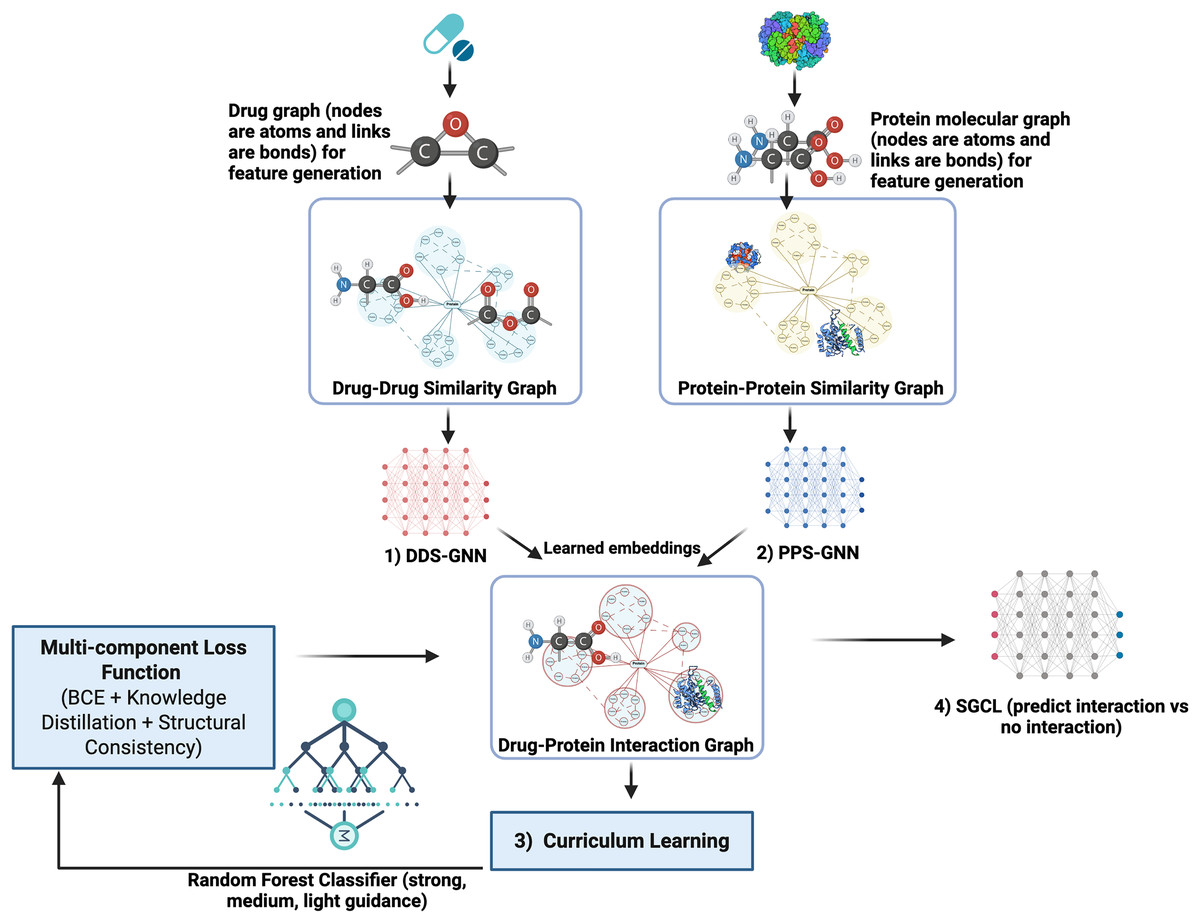
Figure 1: SGCL-DPI architecture: structure-guided curriculum learning framework.
An illustration of the SGCL-DPI, a graph-based framework for drug–protein interaction prediction. It combines similarity graphs processed by GCNs with guidance from a Random Forest model through feature fusion and knowledge distillation. Training follows a two-stage curriculum that transitions from RF-driven learning to GNN-based structural learning, optimized via a multi-component loss.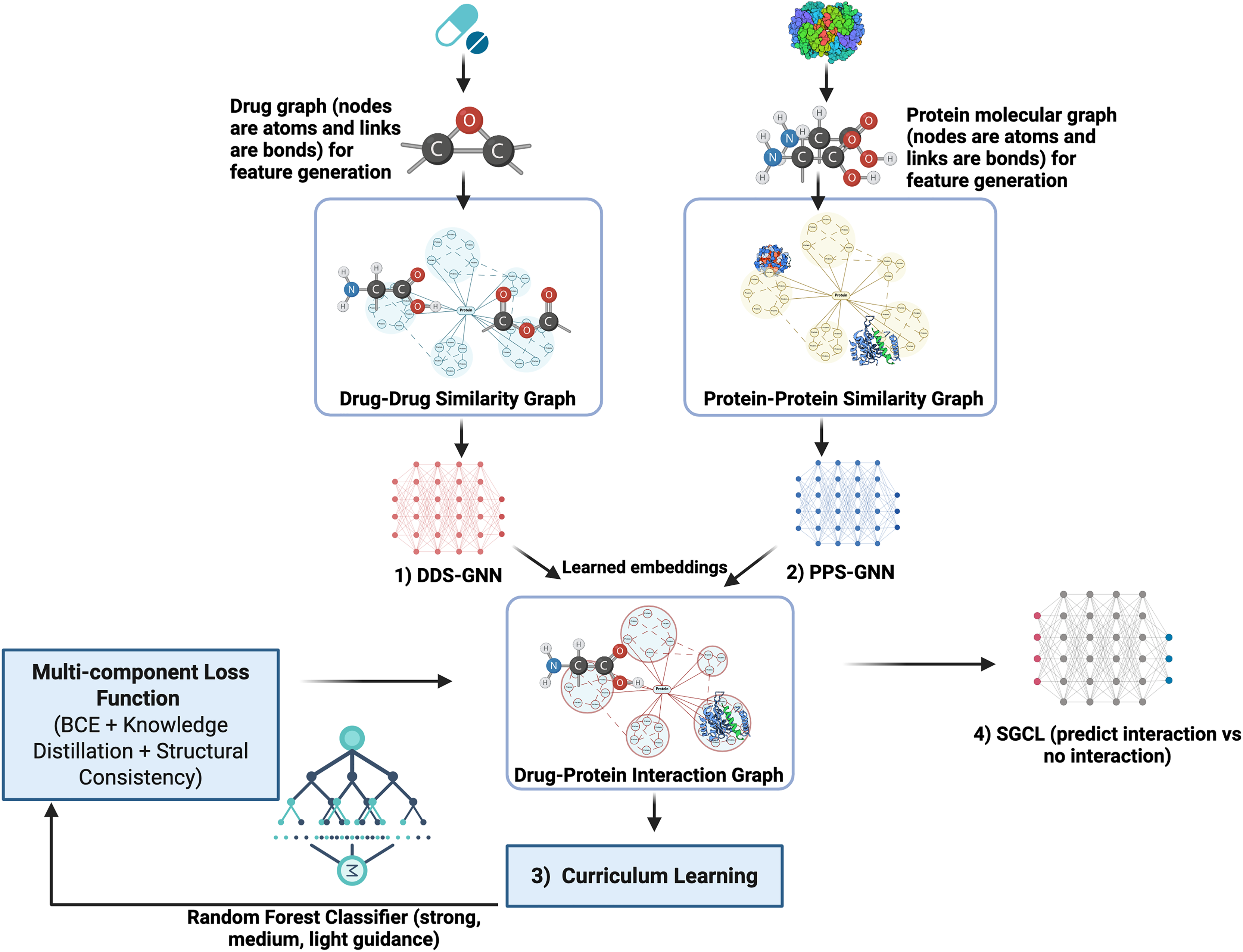
Feature generation and molecular representation
Drug features were generated using a two-component approach: extended-connectivity fingerprints (ECFPs) and chemical descriptors (Soufan et al., 2018). ECFPs were computed using RDKit’s Morgan fingerprint algorithm with radius 2 and 1,024 bits. Chemical descriptors included 15 physicochemical properties: molecular weight, LogP, hydrogen bond donors/acceptors, topological polar surface area, ring count, fraction of SP3 carbons, heavy atom count, rotatable bonds, and partial charge statistics. These descriptors were normalized and combined with ECFPs to create comprehensive molecular representations.
Protein features were generated using a novel combination of sequence-based descriptors. The approach included amino acid composition (AAC), physicochemical properties, and a hashed one-hot encoding scheme. AAC features captured the normalized frequency of each standard amino acid. Physicochemical properties incorporated hydrophobicity, molecular weight, and isoelectric point metrics for each residue, scaled using MinMaxScaler. A fixed-length representation was achieved through a hashing trick applied to one-hot encoded sequences, mapping to a 500-dimensional space while preserving sequence information.
Similarity network construction and integration
Drug-drug (DDS) and protein-protein (PPS) similarity networks were constructed using a weighted combination of feature-based similarities. For drugs, the similarity scores combined Tanimoto similarity of ECFPs (weight = 0.5) with normalized Euclidean distance of chemical descriptors (weight = 0.5). In particular, for two drugs i and j, we compute: (1) Fingerprint similarity as the Tanimoto coefficient between their 1,024-bit ECFPs, and (2) descriptor similarity by taking the Euclidean distance between their descriptor vectors and converting it to a similarity score via a normalized inverse-distance function . We then take a weighted average (we use equal weights 0.5 each by default) of these two measures to obtain a unified similarity score. Using this score, each drug is connected to its k nearest neighbors (highest similarity) in the dataset. The edge weight in the graph is the computed similarity value, reflecting the strength of the relationship. Protein similarities were computed analogously using their sequence-derived features. To manage computational complexity while preserving network information, similarities were computed using a k-nearest neighbor approach (k = 5), with edges established only for similarity scores exceeding 0.5. The analysis generated 14,971,621 drug-drug similarity links and 309,057 protein-protein similarity links.
The resulting similarity networks were integrated into the deep learning architecture through edge-weighted graph convolutional layers. Edge weights, derived from the computed similarity scores, were normalized using L1 normalization and constrained to [0, 1]. These weighted networks were processed through multiple GCN layers, each incorporating layer normalization and Gaussian error linear units (GELU) activation functions. To maintain numerical stability during message passing, safe normalization was implemented with a minimum norm threshold (ε = 1e−12).
This comprehensive feature generation and network construction approach enables effective capture of both local molecular properties and global similarity patterns, while the sparse graph representation achieved through similarity thresholding provides computational efficiency.
To test robustness, additional graphs were generated with (i) cosine similarity at and , (ii) Euclidean similarity ( ), and (iii) Pearson-correlation similarity ( ). All other settings were kept identical. Refer to Table S1 for details.
Graph representations and data encoding
The proposed framework models drugs and proteins as nodes within similarity networks (Meng et al., 2024; Xu et al., 2024), capturing global relationships derived from their chemical and biological descriptors. In the drug–drug similarity graph, each drug is represented as a node. Formally, the graph is defined as
where is the set of drugs, and is a node feature matrix that encodes chemical descriptors such as molecular weight, LogP, and other properties. The edges connect drugs based on similarity metrics, with Tanimoto coefficients computed from molecular fingerprints serving as the basis for quantifying structural similarity.
Proteins are similarly modeled in a protein–protein similarity graph:
Here, denotes the set of proteins, and is the node feature matrix that contains descriptors derived from sequence or structural data. Edges are defined based on similarities computed, for example, from normalized Euclidean distances between physicochemical descriptors.
In both graphs, edge weights are assigned to reflect similarity. For drugs, these weights are derived from Tanimoto coefficients computed on molecular fingerprints. For proteins, a dual approach is employed: sequence alignment scores capture evolutionary and structural relationships, and normalized Euclidean distances of relevant physicochemical descriptors quantify differences in protein properties. This combination produces a robust and comprehensive measure of protein similarity. For numerical stability, the weights are normalized and clipped according to
with .
Graph neural network architecture and message passing
A GNN is employed to learn enriched embeddings for drugs and proteins from the similarity graphs (Hao et al., 2025; Wu et al., 2020). The GNN processes the drug graph (i.e., DDS-GNN-see Fig. 1) and protein graph (i.e., PPS-GNN–see Fig. 1) separately (i.e., a separate GNN encoder for each similarity graph), producing a latent representation for each drug and each protein that accounts for its neighbors. Both graph encoders share a similar architecture: a multi-layer graph convolutional network with normalization and attention mechanisms to ensure stable and informative embeddings.
Each encoder is a stacked GCN with layers (graph convolution operations). For the drug encoder, the input feature size is 1,039 (fingerprint + descriptors); for the protein encoder, it is the length of the protein feature vector (i.e., 523 using a 500-dim hash + 23-dim descriptors). We first project the input features to a lower-dimensional hidden space using a linear layer of 128 dimensions followed by LayerNorm and a GELU nonlinear activation function. This initial projection ensures a manageable embedding size for graph convolution. At each GNN layer , the feature vector of node is updated by aggregating information from its neighbors according to
In this expression, is the feature vector at layer , is the learnable weight matrix, represents the node degree, and are scaling factors computed from edge features. The non-linear activation (implemented as GELU) introduces necessary non-linearity, while normalization by prevents nodes with high connectivity from overwhelming the aggregation process.
Additionally, GCN layers refine these node embeddings. The GCN formulation, incorporating self-loops, is expressed as
where is the augmented adjacency matrix and is its corresponding degree matrix. This formulation effectively aggregates both the local neighborhood and the node’s own features, resulting in robust and discriminative embeddings for subsequent analysis.
Multi-modal integration and feature fusion
The framework integrates features from GNNs with complementary predictions from a RF model that uses traditional molecular descriptors, thereby leveraging both deep and classical machine learning insights.
In our approach, drugs and proteins are processed through separate GNN pipelines to extract nuanced representations from their respective similarity graphs. A GCN layer takes as input a node feature matrix and an adjacency matrix that captures the pairwise similarities between nodes. Conceptually, the code implements an operation analogous to
where ensures numerical stability and bounds the feature values. By normalizing activations, we prevent the embeddings from growing unbounded or becoming too small to be informative.
To obtain fixed-size graph representations, node features are passed through a multi-layer perceptron:
after which attention weights are computed via
The final graph representation is computed as a weighted sum of the node features , where the weights are given by the attention vector . Therefore, nodes with higher attention weights contribute more to the overall graph representation.
To integrate the GNN-derived representation with the RF model’s output, two complementary mechanisms are used. First, direct feature fusion projects both and the RF predictions into a shared latent space via linear transformations and nonlinear activations as follows:
The resulting embeddings are then concatenated or combined through a learnable fusion function, creating a unified representation that benefits from both the GNN’s structural insights and the RF model’s robust, descriptor-based predictions:
which encapsulates both the detailed local structure from the GNN and the robust global patterns from the RF model. Additionally, RF outputs further guide training via a knowledge distillation loss, aligning the GNN’s predictions with those of the RF model.
Curriculum learning strategy
The model is trained using a two-phase curriculum learning (Hacohen & Weinshall, 2019; Soviany et al., 2022) strategy designed to gradually shift emphasis from global patterns captured by RF predictions to the detailed local structural features extracted by the GNN. In the initial phase, known as RF-guided learning, the loss function is configured to heavily weight the RF predictions typically assigning a weight of to this component while the structural component receives a lower weight, such as . This approach allows the model to quickly learn reliable global patterns before focusing on finer details.
As training proceeds, the weight distribution is smoothly adjusted using an exponential schedule:
where is a hyperparameter that determines the rate of transition. This gradual re-weighting minimizes abrupt changes in the learning dynamics, ensuring a smooth transition from RF-guided to structure-guided learning.
Multi-component loss function
The training objective is defined by a composite loss function that simultaneously addresses interaction prediction, RF-guided knowledge distillation, and structural consistency. The primary loss is a weighted binary cross-entropy loss formulated as:
where the adaptive weights are computed by
Here, quantifies the confidence of the RF predictions, and is a scaling hyperparameter that accentuates the focus on samples with higher prediction error.
To ensure the model’s predictions align with those from the RF model, a knowledge distillation loss is introduced:
with the dynamic weights defined as
This dual-threshold strategy ensures that high-confidence RF predictions have a stronger influence on the training process while still incorporating moderately confident signals. Additionally, a structural consistency loss is incorporated to maintain the fidelity of the learned representations with respect to established biochemical and biophysical similarity metrics. This term is calibrated based on empirical similarity distributions.
The overall loss function is then given by
This composite loss function is key to balancing the multiple objectives and ultimately achieving robust performance in drug–protein interaction prediction. is optimized using the AdamW optimizer (Adam with weight decay) for robust convergence. Throughout training, the contribution of each loss component is monitored to ensure that none of them dominates in an unhealthy way (for instance, if remains large when is supposed to be low, that indicates the model is still trying to chase the RF–we avoided this by tuning the decay schedule).
Theoretical rationale for the descriptor-to-structure curriculum
Drug–protein interaction (DPI) prediction involves two information sources for each compound–target pair :
Global descriptors : fixed-length physicochemical fingerprints that encode coarse, low-noise signals (e.g., logP, topological indices).
Structural graphs : high-dimensional, task-specific atom–bond graphs that capture fine-grained three-dimensional complementarity but are harder to model.
Let
be a teacher hypothesis learned by a Random Forest (RF) on .
be the student GNN we ultimately care about.
be the ground-truth interaction label.
At training epoch we minimise the following curriculum objective:
where
is the label-driven term
is the teacher-driven term
-
is a monotonically decreasing curriculum weight with
and .
KD is any differentiable divergence (e.g., KL, soft-MSE) that pushes the student logits toward the teacher’s.
No specific numerical schedule is assumed and any smooth decay that satisfies the boundary conditions can implement the curriculum.
This formulation is equivalent to the earlier formulation , with the identification , , . Thus λ₁ and λ₂ are not tuned independently; they are deterministically governed by the curriculum schedule α(t).
Early epochs are dominated by , whose estimation variance is low because RF ensembles average over descriptors with limited dimension. This regularises the GNN, preventing it from over-fitting the sparse, high-variance structural space. As , the student gradually reduces bias by exploiting structural nuances inaccessible to the teacher. Formally, under the classic bias–variance trade-off, a convex combination of low-variance and low-bias estimators yields an expected risk no worse than either extreme (Hacohen & Weinshall, 2019).
Curriculum learning suggests that presenting samples in order of increasing task difficulty accelerates convergence and improves generalization (Bengio et al., 2009). In DPI, mapping is an easier sub-task (lower VC-dimension) than mapping . The schedule therefore adheres to the self-paced-learning principle that easier hypotheses guide the learner toward regions of parameter space associated with flatter minima.
Model optimization and training protocol
Robust optimization techniques are critical to ensuring the stable convergence of deep graph networks. In this work, several strategies are employed to maintain training stability and efficient convergence.
A cosine annealing schedule with warm restarts is utilized to modulate the learning rate over the course of training. Specifically, the learning rate at time is defined as
and denote the lower and upper bounds of the learning rate, is the number of epochs since the last restart, and is the period of the current cycle. This schedule facilitates periodic exploration of the parameter space, which is beneficial for escaping local minima and promoting a thorough search of the weight landscape. The periodic warm restarts allow the learning rate to reset to a higher value, thereby reintroducing diversity into the optimization process.
To further stabilize the training process, a gradient clipping strategy is applied. This strategy constrains the norm of the gradients during backpropagation to prevent gradient explosion, which is particularly crucial in deep architectures such as those involving graph convolutions.
Formally, gradients are clipped such that , with . This constraint ensures that the parameter updates remain within a reasonable range, preserving both the stability and the efficiency of the optimization process.
In addition to these measures, a batch size of 512 is chosen to balance computational efficiency with the statistical reliability of gradient estimates. Consistent application of layer normalization and safe normalization techniques further ensures that feature distributions remain stable across mini-batches. These normalization techniques help mitigate internal covariate shifts, thereby improving the overall training dynamics.
This methodological framework presents a sophisticated multi-modal approach to drug–protein interaction prediction that goes beyond a simple ensemble of RF and GNN predictions. Rather than merely combining the outputs of two independent models, RF predictions serve as a critical guiding signal throughout the training process. Initially, the RF model—known for its robustness and interpretability based on traditional molecular descriptors—provides reliable global predictions that help the network quickly capture broad interaction patterns. This RF guidance is then gradually phased out in favor of the more detailed local structural features learned by the GNN, achieved via a carefully designed curriculum learning strategy.
By integrating RF predictions through both direct feature fusion and knowledge distillation losses, the approach not only leverages the complementary strengths of classical machine learning and deep learning but also orchestrates a seamless transition from coarse global insights to fine-grained local understanding. This dynamic integration is more than an ensemble strategy; it underpins the training process itself, ensuring that the model converges to a robust representation that is both interpretable and highly predictive.
Performance evaluation metrics
To rigorously evaluate the model’s performance, several standard classification metrics were employed, namely accuracy, precision, recall, F1-score, area under the receiver operating characteristic curve (AUC-ROC), and area under the precision-recall curve (AUC-PR). These metrics provide a comprehensive assessment of the model’s ability to correctly predict drug–protein interactions while accounting for the trade-offs between precision and recall, especially under class imbalance.
Accuracy represents the proportion of correct predictions (both positive and negative) among all predictions made:
Precision is defined as the proportion of correctly predicted positive interactions among all interactions predicted as positive:
Recall quantifies the proportion of true positive interactions that were correctly identified:
The F1-score, which balances precision and recall, is computed as the harmonic mean of the two:
To further characterize overall discriminative performance, the AUC-ROC metric was employed. The AUC-ROC measures the model’s ability to distinguish between positive and negative classes across varying thresholds. Additionally, the AUC-PR metric was computed, as it is more sensitive to performance on imbalanced datasets. The AUC-PR evaluates the trade-off between precision and recall across different threshold settings and provides a more informative summary in settings where true interactions are relatively rare.
Here, TP (true positives) refers to correctly predicted positive drug–protein interactions, FP (false positives) to incorrectly predicted positives, and FN (false negatives) to positive interactions missed by the model. Together, these metrics enable a robust and nuanced evaluation of model effectiveness, balancing both the ability to recover true interactions and to minimize false discoveries.
Model selection rationale
The selection of a graph-based deep learning framework was motivated by the inherent relational structure of drug–protein interaction data, which naturally lends itself to graph representation. By modeling drugs and proteins as nodes in similarity networks, the architecture can effectively capture both molecular structure and relational context. GNNs were therefore selected to enable localized message passing and representation learning across these networks.
The RF classifier was incorporated as a teacher model during training to guide the learning process through knowledge distillation. This choice was based on its strong baseline performance using traditional molecular descriptors, as well as its interpretability and robustness. The integration of RF guidance allowed the model to benefit from handcrafted feature knowledge without requiring a full multi-modal ensemble.
The decision to maintain a single-modality architecture was made, with the goal of evaluating the effectiveness of a focused, structure-guided model without the added complexity of multi-modal integration. This design simplifies implementation and enhances interpretability while still benefiting from molecular feature knowledge through the distillation process. By embedding guidance from the RF teacher during training, the model is able to leverage informative patterns without requiring direct access to raw molecular descriptors at inference time.
Interpretability analysis with integrated gradients
To examine which molecular substructures and protein regions drive SGCL-DPI predictions, we applied integrated gradients (IG), a gradient-based attribution method. IG was computed on the attention-weighted graph embeddings, highlighting the relative contribution of each atom and residue to the final output. The visualization pipeline converts SMILES strings into molecular diagrams and color-codes atomic contributions (red for strong positive attribution, blue for negative). This allows direct inspection of how the model propagates information across the drug and protein graphs, providing insight into its decision-making process. Details are provided in Article S1.
Evaluation methods
To ensure a thorough and transparent assessment, the following evaluation strategies were applied in this study: (1) Baseline comparison using a RF model trained on traditional molecular descriptors, (2) generalization testing through the “hard split” protocol introduced by Watanabe, Ohnuki & Sakakibara (2021), (3) comparative analysis against single- and multi-modality baselines reported in prior literature, (4) ablation studies to examine the contribution of individual loss components and architectural elements, and (5) curriculum learning sensitivity analysis to explore the effect of varying the knowledge distillation weight (Alpha).
The performance and generalization capability of the proposed SGCL-DPI framework were evaluated through a comprehensive set of experimental strategies. As an initial baseline, a RF model trained on traditional molecular descriptors was employed. This model, built using established cheminformatics features, served as a classical benchmark and was assessed across 10 random splits of the BindingDB dataset to provide robust statistical averages for comparison.
To test model robustness under realistic and challenging conditions, the evaluation incorporated the “hard split” protocol introduced by Watanabe, Ohnuki & Sakakibara (2021). In this setting, no drugs or proteins appearing in the training folds are allowed in the test folds, thereby simulating scenarios involving entirely novel molecular entities. This approach is widely recognized for its rigor and relevance to drug discovery tasks.
Comparative analysis was conducted using baseline models reported in the literature, particularly those from Watanabe, Ohnuki & Sakakibara (2021). These included single-modality models utilizing only molecular features or only network-based embeddings, as well as a more complex integrated model that combines both data types. This comparison established a contextual benchmark for assessing the SGCL-DPI model’s standing among contemporary deep learning approaches.
To isolate the contribution of each architectural and training component, several ablation studies were performed. These experiments examined model variants trained using only individual loss components including weighted binary cross-entropy (BCE), knowledge distillation (KD) from the RF teacher, or structure consistency loss, as well as a version that excluded the graph encoder. The resulting performance differentials provided insight into the importance of each component.
The effect of curriculum learning parameters was also investigated by varying the weighting factor (Alpha) associated with the KD loss during training. Different Alpha values were tested to determine the optimal balance between guidance from the RF teacher and autonomous learning within the graph-based architecture.
All model variants were evaluated on held-out validation sets using standard classification metrics, including accuracy, precision, recall, F1-score, AUC-ROC, and AUC-PR. These metrics offered a comprehensive view of each model’s predictive behavior across different evaluation scenarios.
Performance and scalability
Graph construction represents the primary computational bottleneck in SGCL-DPI, as it requires exhaustive pairwise similarity calculations across all drug–drug and protein–protein combinations. To mitigate this cost, precomputed similarities are cached and stored using efficient data structures; RDKit handles fingerprint generation, while NumPy is used for descriptor distance computations. Parallel execution on an NVIDIA A100 GPU reduces this preprocessing to a one-time operation, after which persisted graphs enable rapid training. On a dataset with tens of thousands of interactions, SGCL-DPI completes over 100 epochs using a cosine learning-rate schedule in approximately 16 min per run on the same GPU. Evaluation on a standard laptop (16 GB RAM, quad-core Intel Core i7) confirms that, with precomputed graphs, both training (with a reduced number of epochs) and inference are feasible without specialized hardware. The PyTorch/PyG implementation supports fully vectorized GNN operations and dynamic computation of the multi-component loss, maintaining scalability and efficiency in typical research settings. In a production setting, graph construction can be incremental, only the similarity rows and columns for newly added compounds or targets need to be computed, so the preprocessing cost is spread over time and typically falls to a few seconds per update.
Results
Random forest baseline performance: revealing the potential of traditional molecular descriptors
As shown in Table 1, the RF classifier using traditional molecular descriptors achieved exceptionally high performance on the BindingDB benchmark. In particular, the RF model attained an average AUC of 99.18% and AUPR of 99.14% across 10 random splits, along with a Precision of ~96.8% and Recall of ~95.7%, yielding an F1-score of ~96.2%. This outperforms several deep learning models reported in the literature on the same dataset. For example, GraphDTA (which employs graph neural networks on molecular graphs and CNNs on protein sequences) achieved an AUC of about 93.6% and AUPR of 93.4%. Similarly, the TransformerCPI model (a transformer-based sequence-only approach) reached roughly 95.7% AUC and 95.8% AUPR. Even BridgeDPI reported an AUC/AUPR of 97.5%/97.3%, which, while high, is still lower than the RF’s performance in our experiments.
| Model (BindingDB) | Precision (%) | Recall (%) | F1-score (%) | AUC-ROC (%) | AUPR (%) |
|---|---|---|---|---|---|
| Random forest (Descriptors) | 96.77 (±0.17) | 95.65 (±0.12) | 96.21 (±0.09) | 99.18 (±0.03) | 99.14 (±0.05) |
| GraphDTA (Nguyen et al., 2021) | – | – | – | 93.6 | 93.4 |
| TransformerCPI (Chen et al., 2020) | – | – | – | 95.7 | 95.8 |
| BridgeDPI (Wu et al., 2022) | – | – | – | 97.5 | 97.3 |
Notably, these results were achieved without using any graph neural networks, protein sequence models, or other complex multi-modal frameworks. The RF model relied solely on well-established molecular descriptors (traditional chemical features), yet it matched or exceeded state-of-the-art performance. This highlights the surprising strength of carefully engineered classical descriptors in this context. They appear to capture the key determinants of binding interactions effectively enough that a simple ensemble classifier can leverage them to rival deep learning models. In other words, for the BindingDB dataset, the added complexity of deep neural networks (GNNs, transformers, etc.) did not translate into better performance than the descriptor-based approach, underlining how informative the descriptors are for this task.
Comparison with Random Forest baseline–hard dataset
To better assess robustness under more realistic and demanding conditions, we evaluated SGCL-DPI and baseline methods on a harder test set. On the hard test set (see Materials and Methods), the proposed graph-based model achieves an accuracy of ~76.3%, slightly higher than the RF baseline’s ~75.3% (Table 2). More importantly, our model exhibits a much better balance between precision and recall. It attains recall = 73.00% (±6.68), meaning it correctly recovers a large fraction of true drug–protein interactions. This recall is over 2.2× higher than that of the RF baseline (32.64% ± 9.53), which struggled to identify positive interactions. The RF model’s precision is indeed higher (82.52% vs. 62.24%), indicating it makes fewer false-positive predictions, but this comes at the cost of missing most true interactions. The proposed model’s more moderate Precision (62.24% ± 3.25) coupled with its strong recall yields a substantially better F1-score (67.06% ±3.50) compared to the RF’s F1 (46.20% ± 10.35). In other words, our method achieves a more favorable precision–recall trade-off, improving F1 by ~21 points. This suggests that the graph-based approach is more effective at finding true interactions without being overly conservative. We note that the AUC-ROC values of the two models are practically equivalent (≈82.3% vs. 82.1%), indicating that overall ranking ability (in terms of true-positive rate vs. false-positive rate across thresholds) is comparable. However, as Watanabe, Ohnuki & Sakakibara (2021) emphasize, the AUC-PR is a more informative metric on class-imbalanced problems like this (where true interactions are relatively scarce) (Watanabe, Ohnuki & Sakakibara, 2021). By this measure, our model’s performance (AUC-PR ≈71.7%) is on par with the RF (72.6%), suggesting that both models achieve a similar area under the precision–recall curve despite their different operating points. The key distinction is that our model operates at a higher-recall point on that curve, capturing far more positives. This balanced performance is critical in practical settings where missing potential interactions (false negatives) is as problematic as having some false positives.
| Method | Accuracy | Precision | Recall | F1-score | AUROC | AUPR |
|---|---|---|---|---|---|---|
| SGCL-DPI | 76.26% ± 2.06 | 62.24% ± 3.25 | 73.00% ± 6.68 | 67.06% ± 3.50 | 82.33% ± 2.02 | 71.69% ± 4.77 |
| RF baseline (Molecular descriptors only) |
75.30% ± 3.23 | 82.52% ± 6.79 | 32.64% ± 9.53 | 46.20% ± 10.35 | 82.12% ± 2.21 | 72.58% ± 4.29 |
|
Watanabe, Ohnuki & Sakakibara (2021)–Molecular (Sequence + Structure only) |
80.6% ± 2.0 | – | – | 66.2% ± 3.8 | 85.1% ± 2.3 | 77.0% ± 2.3 |
|
Watanabe, Ohnuki & Sakakibara (2021)–Network (Interactome only) |
78.4% ± 2.3 | – | – | 60.1% ± 5.7 | 78.0% ± 5.1 | 70.6% ± 4.0 |
Critically, we acknowledge that the improved recall of the proposed model comes with somewhat lower precision than the RF. This indicates a higher false-positive rate, which is a trade-off to gain more true hits. Depending on the application, one might adjust the decision threshold to tune this balance; however, the substantially higher F1 of our method demonstrates that overall it achieves a better compromise between precision and recall than the RF baseline. A threshold sweep (see Fig. S1) shows that while both models reach a similar peak F1 of ≈ 0.70 at a narrow threshold (~0.25), the Random Forest baseline’s F1 drops sharply thereafter, whereas SGCL-DPI maintains F1 ≥ 0.50 across a broad threshold range (0.25–0.70), demonstrating that the balanced precision–recall performance is not tied to a single threshold. In summary, compared to a traditional machine learning baseline using the same input features, the proposed graph-based model delivers more robust and comprehensive predictions, identifying many more true interactions while maintaining reasonable precision.
Comparative analysis with baseline models and Watanabe, Ohnuki & Sakakibara’s (2021) approaches
The work of Watanabe, Ohnuki & Sakakibara (2021) was selected as a benchmark due to its rigorously defined hard dataset and comprehensive evaluation of deep learning models. While our RF-based approach outperformed several recent GNN methods on BindingDB, Watanabe’s framework presented a more challenging and widely recognized generalization test. Although reproducing their experiments was not feasible due to difficulties running their published code, their dataset and methodology remain influential and were instrumental in guiding the comparative evaluation in this study.
The performance of the proposed graph-based model was compared against the benchmarks reported by Watanabe, Ohnuki & Sakakibara (2021) on the hard split derived from the STITCH database (see Fig. 2). Watanabe, Ohnuki & Sakakibara (2021) presented three variants in their work: an integrated model (combining molecular sequence/structure features with network context), a single-modality model based on molecular features alone, and a network-only model. Notably, the present work focuses on a single-modality approach, wherein the drug–protein interaction graph serves as the sole data source; however, it benefits indirectly from molecular features via a RF module integrated through curriculum learning. Unlike traditional ensemble methods, the RF component in this approach is not used for independent prediction; instead, its output is used for knowledge distillation and feature fusion during training, thereby informing the graph-based predictor without requiring the simultaneous optimization of heterogeneous data sources.
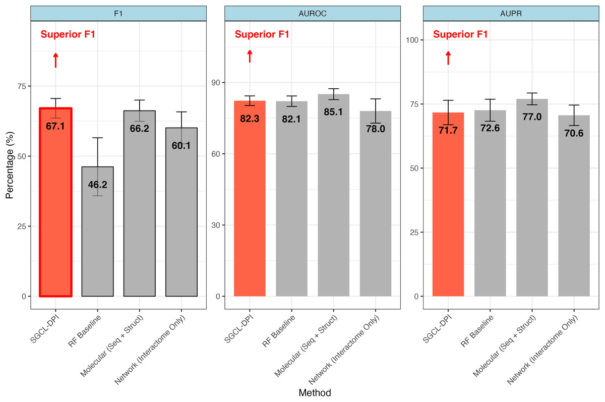
Figure 2: Comparative performance of SGCL-DPI vs. single-modality baselines on the STITCH hard dataset.
The SGCL-DPI framework with three single-modality baselines: a Random Forest (RF) trained on molecular descriptors, a molecular-only deep model (sequence + structure), and a network-only model based on interactome data. SGCL-DPI achieves the highest F1-score (67.1%), indicating a superior balance between precision and recall. While AUROC and AUPR are comparable across methods, SGCL-DPI consistently matches or closely approaches state-of-the-art performance, demonstrating its effectiveness under strict generalization conditions without full multi-modal integration. Error bars reflect performance variation across cross-validation folds.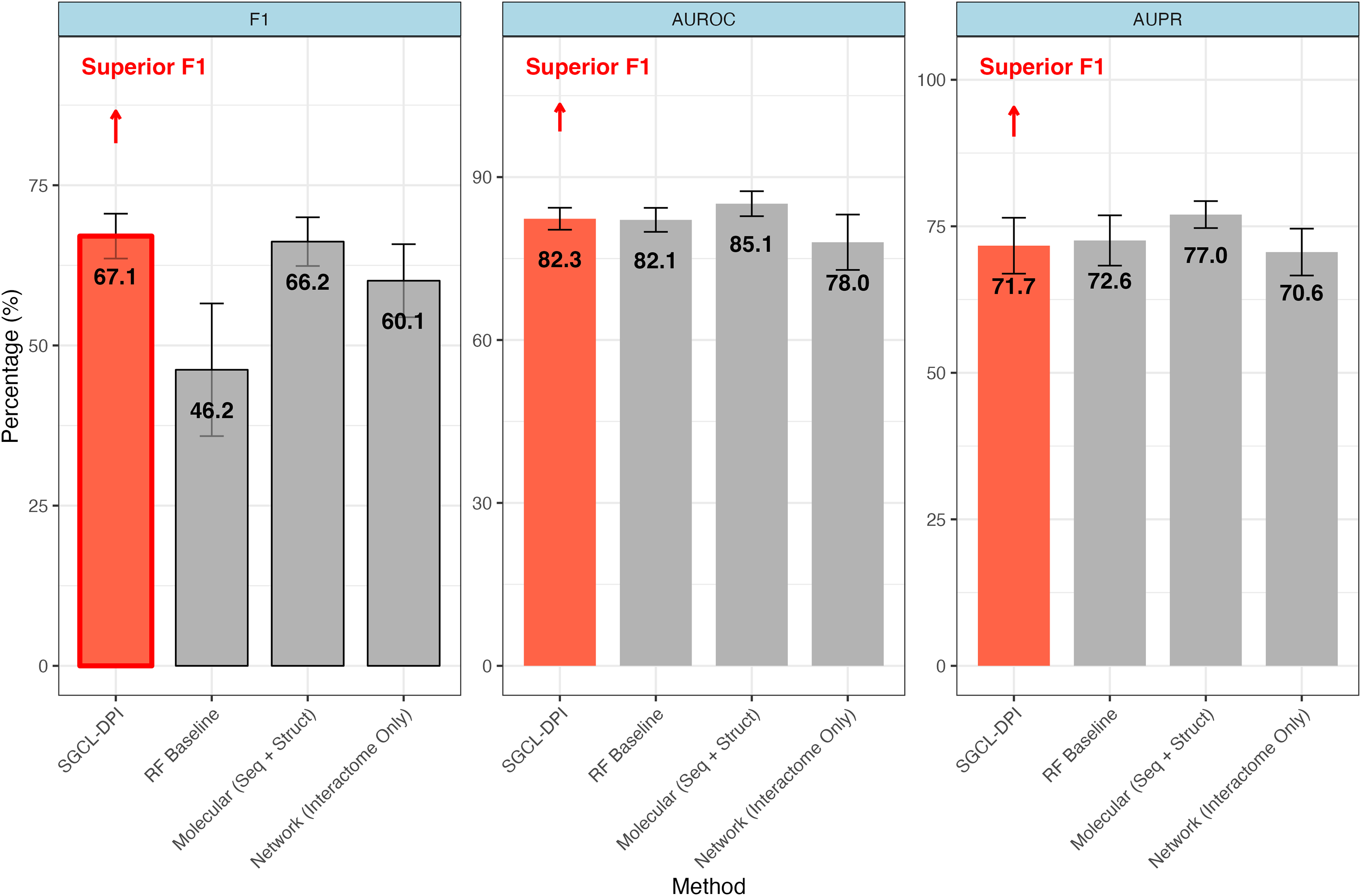
Performance against single-modality network baseline
The proposed graph-based model markedly outperforms Watanabe, Ohnuki & Sakakibara’s (2021) single-modality network approach in most metrics. In particular, it achieves a higher F1-score (67.06% vs. 60.1%; an improvement of about 11.6%) and AUPR (71.69% vs. 70.6%) than the purely network-driven model of Watanabe, Ohnuki & Sakakibara (2021) despite a slightly lower overall accuracy (76.26% vs. 78.4%) (see Table 2). This improvement indicates that our method’s incorporation of molecular information provides an advantage over an interactome-only strategy. By integrating knowledge from molecular descriptors, the proposed method detects more true drug–protein interactions (recall 73.00% vs. an implied lower recall for the network baseline) while maintaining a reasonable precision, thus yielding a better balance between precision and recall. In contrast, Watanabe’s network-only model, which relies solely on similarity networks of proteins and compounds, appears to miss many interactions (lower recall), resulting in a diminished F1-score. These gains indicate that the graph-based formulation, even when operating as a single-modality approach, is able to capture more nuanced patterns of interactions—most likely by exploiting local graph topology and higher-order connectivity—than a pure network embedding method.
Performance against single-modality molecular baseline
The SGCL-DPI framework demonstrated competitive performance when compared with the single-modality molecular baseline reported by Watanabe, Ohnuki & Sakakibara (2021) which leveraged protein sequence and compound structure features without incorporating interaction networks. On the STITCH hard split, SGCL-DPI achieved an F1-score of 67.1%, slightly surpassing the molecular baseline’s 66.2%, representing an improvement of approximately 1.4%. Although the molecular baseline reported higher AUROC (85.1% vs. 82.3%) and AUPR (77.0% vs. 71.7%), the higher F1-score of SGCL-DPI highlights a more favorable balance between precision and recall. This advantage is particularly noteworthy considering that SGCL-DPI operates without direct access to raw molecular sequences or structures, relying instead on similarity networks and knowledge distillation from a RF teacher model. These findings underscore the effectiveness of SGCL-DPI’s graph-based design and training strategy in capturing predictive interaction patterns with minimal feature complexity.
SGCL-DPI vs. integrated multi-modal models
Watanabe, Ohnuki & Sakakibara’s (2021) integrated model, which fuses molecular sequence/structure features with network context, achieved an AUROC of 88.2% (±3.5), an AUPR of 83.4% (±4.1), and an F1-score of 71.4% (±6.4). Although the integrated model outperforms the proposed approach in absolute terms, it should be noted that the present study deliberately adheres to a single-modality design. The goal is to demonstrate that even without the complexity of integrating multiple data modalities (i.e., protein sequences, chemical structure features, and extensive interactome data) a focused graph-based method, when augmented via curriculum learning with an RF-based molecular guidance, can yield competitive performance. In fact, the proposed model’s F1-score (67.06%) attains approximately 94% of the value achieved by the integrated model, and its AUROC is within 6 percentage points. These findings highlight that a streamlined, single-modality approach can capture a significant portion of the predictive signal, while preserving simplicity and reducing computational and architectural complexity.
While the obvious extension of integrating complementary data types (e.g., through fully ensemble methods) remains a promising avenue for future research, the current work demonstrates that a graph-based method using only the drug–protein interaction network enhanced indirectly with molecular feature guidance via a curriculum learning process achieves a robust balance between precision and recall. The strength of the method lies in its ability to substantially outperform conventional network-only methods and to deliver results competitive with more complex multi-modal systems, despite not utilizing a full ensemble strategy. This single-modality approach offers practical advantages including reduced model complexity, easier interpretability, and greater ease of deployment in resource-constrained settings.
Loss function ablation and model variants
To evaluate the contribution of each loss component and the graph encoder, we conducted ablation experiments on the hard split of the STITCH dataset. Table 3 summarizes key performance metrics (accuracy, precision, recall, F1-score, AUC-ROC, AUC-PR) for the full multi-component model (using weighted binary cross-entropy (BCE), knowledge distillation (KD) from the Random Forest, and structure consistency loss) compared to several ablated variants using only weighted BCE loss, only KD loss, only structure consistency loss, and a no-graph variant combining BCE + KD losses without the graph encoder (no GNN-based structure learning).
| Model (Loss configuration) | Accuracy | Precision | Recall | F1 | AUC-ROC | AUC-PR |
|---|---|---|---|---|---|---|
| Full (BCE + KD + Struct) | 76.26 ± 2.06 | 62.24 ± 3.25 | 73 ± 6.68 | 67.06 ± 3.5 | 82.33 ± 2.02 | 71.69 ± 4.77 |
| BCE only (Graph only) | 69.31 ± 20.17 | 68.86 ± 20.55 | 58.91 ± 23.28 | 57.82 ± 5.78 | 81.05 ± 2.25 | 71.63 ± 4.58 |
| KD only (RF distillation only) | 33.22 ± 0.6 | 33.22 ± 0.6 | 100 ± 0 | 49.87 ± 0.67 | 82.32 ± 2.01 | 73.37 ± 6.05 |
| No GNN (BCE + KD, no graph) | 50.22 ± 22.8 | 36.45 ± 29.14 | 71.6 ± 43.88 | 43.74 ± 25.65 | 46.28 ± 30.17 | 37.59 ± 22.22 |
| Structure only (Struct loss) | 77.87 ± 1.84 | 76.62 ± 6.03 | 48.73 ± 3.7 | 59.39 ± 2.75 | 81.93 ± 1.83 | 71.93 ± 3.86 |
Note:
The highest values for F1 and AUC-PR are bolded.
From these results, the full model clearly achieves the strongest overall performance, with the highest F1-score (67.06%) and AUC-ROC (82.33%). This indicates that all loss components together produce a synergistic effect, improving both precision and recall compared to any single-loss model. In contrast, using only one loss type led to significant drops in performance. For example, a model trained only with weighted BCE (i.e. using graph-based learning on labels alone, without KD or structure loss) reached an F1 of 57.82%, notably lower than the full model.
The KD-only model (trained solely by distilling the Random Forest’s predictions, without direct supervision on the interaction labels) achieved perfect recall (100%) at the expense of lower precision (33.22%). By predicting a large number of positives, it successfully captured nearly all true interactions, but at the cost of introducing many false positives. This behavior suggests that while knowledge distillation can effectively transfer general decision patterns, relying solely on the teacher’s outputs without ground-truth labels can cause the student model to overgeneralize. These findings highlight the importance of complementing distillation with task-specific supervision to achieve more balanced and reliable predictions. Notably, the KD-only model’s AUC-ROC (82.32%) and AUC-PR (73.37%) were very close to those of the full model, indicating that the teacher’s knowledge remains valuable, particularly for ranking predictions even when not directly trained on the interaction labels.
Including the structure consistency loss on its own (without BCE or KD) resulted in moderate predictive performance (Table 3). This variant achieved a relatively high accuracy (77.87% ± 1.84) and precision (76.62% ± 6.03), but much lower recall (48.73% ± 3.7), indicating a tendency to make confident but conservative predictions. The F1-score (59.39% ± 2.75) reflects this imbalance. While the model performed reasonably well in ranking (AUC-ROC: 81.93% ± 1.83, AUC-PR: 71.93% ± 3.86), its lack of direct supervision likely limited its ability to generalize across diverse interaction types. This suggests that while the structure loss offers useful regularization, it is insufficient on its own to drive robust interaction prediction. These findings reinforce the role of the structure loss as a complementary signal, best used in conjunction with a primary supervised objective such as BCE or knowledge distillation.
Crucially, removing the graph encoder degraded performance significantly. The No GNN variant (which uses both BCE and KD losses but no graph-based similarity learning) achieved an F1 of 43.74% and AUC-PR of 37.59%, considerably lower than the full model. Both precision and recall dropped relative to the full model, indicating that structural learning via the GNN is important for generalization. Without the graph, the model cannot leverage similarities between drugs or between proteins; effectively it must treat each entity in isolation (aside from what the RF teacher provides). This leads to a notable loss in recall on the hard split, because the model struggles with novel drug–protein combinations that were not seen during training. In contrast, the full graph-based model can propagate interaction signals across similar drugs and proteins, enabling it to catch interactions involving new compounds by analogy to known ones. For example, if a new drug has a close structural analog in the training set that interacts with a given protein, the GNN can transfer that relational signal through the drug similarity graph, something the no-graph model cannot do. The higher AUC-PR for the full model compared to the no-GNN model (71.69 vs. 37.59) reflects this advantage, especially in identifying the minority positive class instances. We also ablated the knowledge-distillation term while keeping the GNN intact (see row ‘BCE only’ in Table 3). Eliminating RF guidance lowered F1 on STITCH-hard from 67.06 ± 3.5% to 57.82 ± 5.8% and reduced Recall by 14%, confirming that a descriptor-first curriculum is critical for capturing difficult, cross-domain interactions.
Overall, these ablations demonstrate that each component of the proposed approach contributes meaningfully to performance. The weighted BCE loss serves as the core learning signal for interaction prediction, the KD loss transfers useful guidance from the RF teacher to enhance both precision and recall, and the structure consistency loss adds a regularization effect that supports more stable learning. Together, these components enable the model to strike a better balance between false positives and false negatives than any individual part alone. By combining teacher knowledge with graph-based structural learning, the full model achieves improved generalization and a more effective precision–recall trade-off on this challenging prediction task.
Importantly, the proposed model attains this performance with a single-modality architecture. It does not incorporate the chemical descriptors or protein features directly into a multi-branch neural network, nor does it ensemble the RF with the GNN at inference. Instead, molecular feature knowledge is infused through distillation during training, allowing the final model to remain focused on graph-based representations. This design means that at test time the model uses only the similarity graphs (and no external features or ensemble voting), yet it performs on par with or better than approaches that explicitly fuse multiple data types. The strong F1 and AUC-PR achieved without late-stage feature fusion highlight the efficiency of this strategy. We gain the informative signal of descriptors in an interpretable way (via the teacher’s guidance) while avoiding the complexity of full multi-modal integration.
Impact of curriculum learning parameters on model performance
We observed differential performance across three curriculum learning setups (Alpha = 20, 35, 50) on drug–protein interaction prediction F1-scores, highlighting the influence of curriculum parameter tuning (see Fig. 3). In this context, Alpha denotes the weighting factor applied to the knowledge distillation loss from the RF model during the initial training phase. Larger Alpha values place stronger emphasis on aligning the graph neural network’s predictions with those of the RF teacher, thus providing more global guidance at early stages of learning. These values were chosen based on initial experimentation, where smaller Alpha values failed to provide adequate RF supervision to guide early learning.
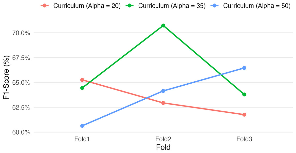
Figure 3: Effect of curriculum learning weight (Alpha) on F1-score across folds.
Varying the RF loss weight (α = 20, 35, 50) under different curriculum learning setups affects the F1-score over three cross-validation folds. The results highlight that alpha = 35 yielded the highest F1 performance on Fold 2, while alpha = 50 showed improved consistency across folds. These folds were chosen as they reflect varying behaviours. These findings underscore the sensitivity of the SGCL-DPI framework to curriculum scheduling and suggest that moderate RF guidance may strike the best balance for generalization. Further tuning could improve stability and predictive performance.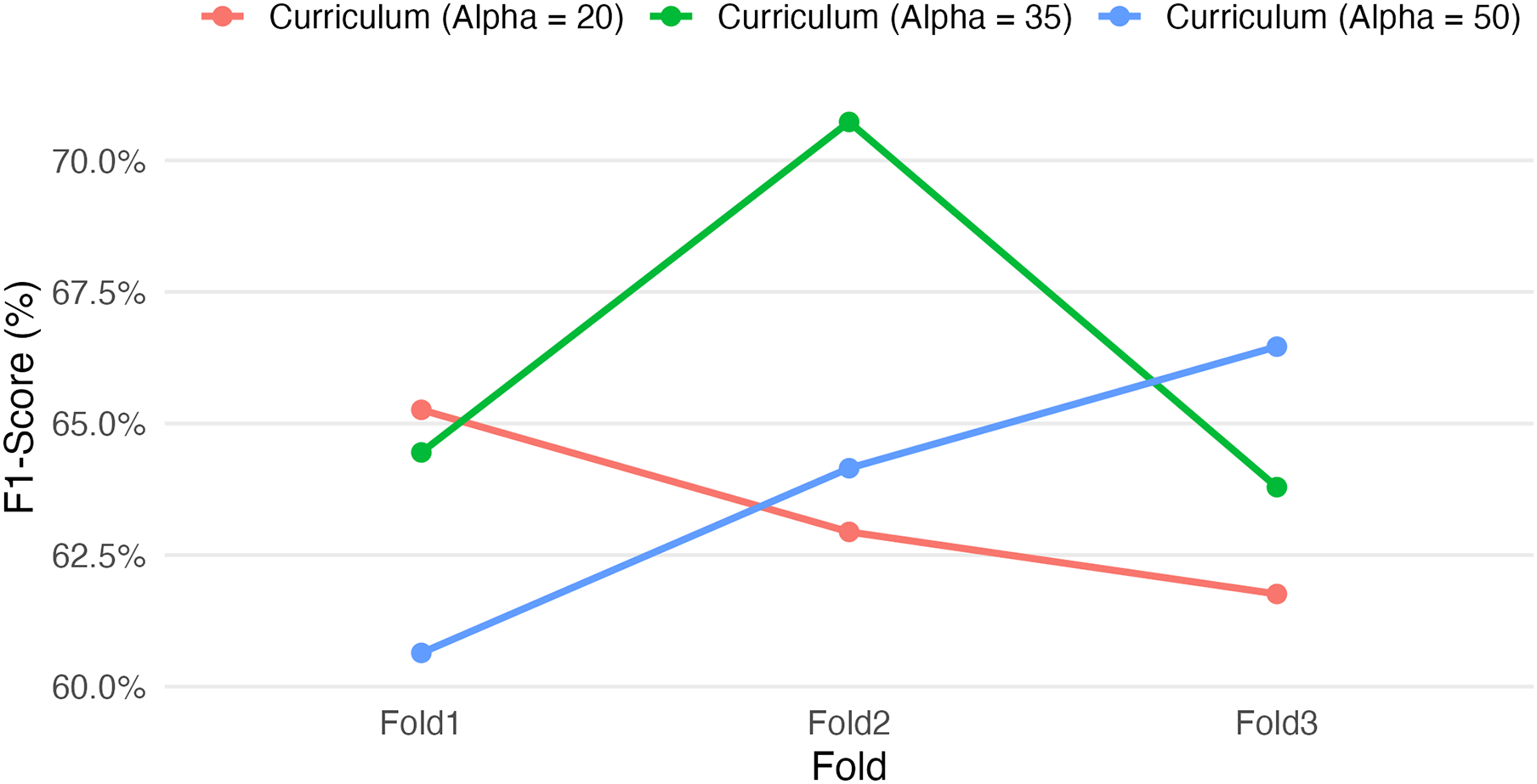
Among these, the intermediate setting (Alpha = 35) yielded the highest single-fold F1-score (70.73% on Fold 2) as well as the highest overall mean performance (~66.3%, vs. ~63–64% for the other setups). These results suggest that a moderately paced curriculum may be optimal for this task. However, the Alpha = 35 configuration also showed greater variability between folds (e.g., 64.45% on Fold 1 vs. 70.73% on Fold 2) relative to the other configurations (with ~6–7 percentage-point F1 swings across folds, compared to ~3–5 for the others), indicating a sensitivity to training data splits or initial conditions. In comparison, the more conservative curriculum (Alpha = 20) produced more consistent F1-scores across folds (65.26%, 62.94%, 61.76%) but did not achieve the same peak performance, while the more aggressive curriculum (Alpha = 50) had intermediate outcomes (60.64–66.46% across folds). Notably, each fold’s highest score was achieved with a different Alpha value (Alpha=20 in Fold 1, 35 in Fold 2, 50 in Fold 3), underscoring the non-monotonic influence of the curriculum parameter on performance. This sensitivity and the fact that only the appropriately tuned value (Alpha = 35 in this experiment) delivered a pronounced performance gain underscore the importance of careful hyperparameter optimization. Although these results are preliminary, they demonstrate that tuning curriculum learning parameters can yield meaningful gains in predictive performance. Given the observed sensitivity, a more exhaustive hyperparameter search could be pursued in the future to further refine these gains and validate the robustness of the approach.
Qualitative model interpretation
Atom-level attributions were next examined using IG (see Article S1). In a true-positive example, the attributions appeared sharply localized with high intensity over biologically meaningful functional groups, including a phosphate moiety, substituted aromatic rings, and polyhydroxy regions. This pattern suggests that the model bases correct predictions on chemically relevant substructures. In contrast, a false-positive case revealed diffuse, low-contrast attributions scattered across non-specific hydroxyl chains, lacking any dominant substructure to support the model’s high predicted probability which is indicative of over-generalization from widely occurring motifs. Collectively, these examples demonstrate how interpretability analyses can differentiate between well-grounded and unreliable predictions in SGCL-DPI.
Discussion
The proposed framework achieves exceptional predictive performance using a surprisingly simple feature set. On the BindingDB benchmark, it attains near-perfect results using traditional molecular descriptors with a Random Forest classifier, outperforming state-of-the-art deep learning methods that employ more complex, multi-modal feature extraction. Its competitive performance on the challenging STITCH-hard dataset further supports that a well-designed descriptor-based approach can effectively drive drug–protein interaction prediction.
A notable strength of the method is its focused simplicity. Unlike multi-modal models that rely on diverse data sources and complex ensembles, this approach leverages a single modality using compound descriptors and then, transfers knowledge from an RF to a graph neural network via a carefully designed curriculum learning strategy. This streamlined process minimizes data requirements and computational overhead while still capturing higher-order interaction patterns and achieving robust generalization.
Ablation studies provide clear insights into the contributions of individual components. The experiments demonstrate that removal of the graph encoder or the knowledge distillation signal substantially impairs model performance on novel compounds and proteins, highlighting the complementary roles of the weighted binary cross-entropy loss, KD loss, and graph-based regularization. In isolation, while the KD component boosts recall by recovering most true interactions, it also tends to over-predict, thus reducing precision, emphasizing the need for a balanced combination of all learning signals.
Future directions for this work include extending the current framework toward deeper integration of multi-modal learning without compromising its efficient architecture. For example, although the present model already encodes meaningful protein features including amino acid composition and physicochemical properties into the similarity graphs, future enhancements could involve richer representations, such as pretrained protein language model embeddings or structural domain profiles. A more comprehensive distillation scheme could also be explored, where separate teacher models are trained independently for the drug and protein modalities and their signals are jointly distilled into the graph-based learner. This would move the framework closer to multi-modal architectures while retaining the benefits of staged curriculum learning and interpretable molecular guidance. Such improvements could further enhance predictive performance, especially in challenging generalization settings like unseen compound–protein pairs.
Another promising direction involves the joint optimization of feature representations and graph topology. Rather than relying on a fixed similarity graph constructed from static descriptors, future work could explore trainable, adaptive graph-building techniques that dynamically update inter-node connectivity based on intermediate training signals. For example, future work could employ graph-transformer layers or three-dimensional GNNs that are explicitly designed to respect any rigid rotation or translation of a molecule in 3-D space. This would enable the model to learn an implicit kernel that reflects functional or structural proximity beyond hand-crafted similarities. Complementary strategies such as self-supervised pretraining on the similarity graphs via graph autoencoders or contrastive learning may further enhance representation quality and improve downstream predictive performance. Additionally, lightweight ensemble-based distillation, in which multiple specialized teacher models contribute complementary knowledge to a unified student model, offers another pathway for boosting accuracy and robustness without significantly increasing inference cost. This direction could bridge the gap between classical interpretable models and more comprehensive deep architectures, contributing to more generalizable and efficient solutions for drug–target interaction prediction.
Conclusions
This work introduced SGCL-DPI, a structure-guided curriculum learning framework that validates the hypothesis that a single-modality graph-based model can reach competitive performance in drug–protein interaction prediction when guided by classical machine learning knowledge. Our results showed that even a simple RF trained on traditional molecular descriptors can be remarkably effective on a benchmark like BindingDB, outperforming several deep learning baselines in isolation. By integrating the RF’s knowledge in a two-phase curriculum, the SGCL-DPI model surpassed the performance of a graph-only GNN baseline and ultimately achieved higher F1-scores and recall than either the RF or the standalone GNN. Notably, on a challenging evaluation with completely unseen compounds and proteins (a hard split derived from STITCH), SGCL-DPI outperformed Watanabe, Ohnuki & Sakakibara’s (2021) network-only DTI model and approached the accuracy of their molecular feature-based model, all while using a simpler architecture.
These findings underscore that a carefully guided single-modality approach can capture much of the benefit of multi-modal frameworks. The curriculum learning strategy first distilling predictions from the RF and then fine-tuning with structural regularization enabled SGCL-DPI to combine the strengths of classical and deep learning methods. Ablation studies confirmed that each component of our design is important where removing the knowledge distillation or the structure-based loss led to notable drops in performance, and eliminating the GNN’s structural learning caused a dramatic decline, emphasizing the critical role of network topology. Overall, SGCL-DPI provides a favorable balance between precision and recall, generalizes well to novel protein–compound pairs, and remains relatively interpretable and efficient due to its reliance on a transparent RF guidance and a streamlined model design.
Nevertheless, there is room for further improvement. The AUC-PR achieved by SGCL-DPI, while competitive, was slightly lower than that of some fully integrated multi-modal models, indicating that certain synergies between molecular descriptors and interactome data are not yet fully exploited. Future work will explore a tighter integration of the RF-derived features with the graph-based model. For example, through joint optimization or feature fusion to harness these synergies and further boost predictive power. Another promising direction is to incorporate richer structural information (e.g., 3D protein pocket features) into the curriculum, which could enhance the model’s ability to capture binding mechanisms. Finally, evaluating SGCL-DPI on additional challenging benchmarks (such as those with novel chemical scaffolds or distinct protein families) will be important to verify and extend its generalizability to new domains, guiding subsequent refinements of this approach.
Supplemental Information
F1 Score Sweep on STITCH-Hard.
The Random Forest baseline (blue) and SGCL-DPI (orange) are evaluated by varying the classification threshold from 0.05 to 0.95. Both models achieve peak F1 performance at a threshold around 0.25, with SGCL-DPI maintaining superior stability and higher scores at moderate thresholds, while Random Forest performance degrades more rapidly as the threshold increases.
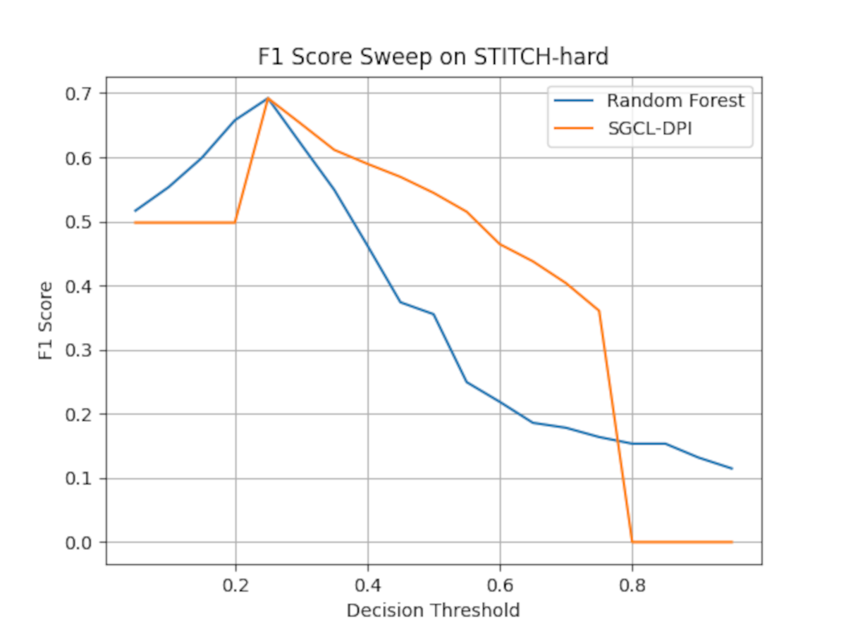
Robustness of SGCL-DPI to alternative graph-construction strategies (one validation fold, STITCH-hard split).
Performance is reported after retraining the model with different similarity metrics or