
A lightweight PCB defect detection method based on group convolution and adaptive pruning
- Published
- Accepted
- Received
- Academic Editor
- Paulo Jorge Coelho
- Subject Areas
- Artificial Intelligence, Computer Vision, Neural Networks
- Keywords
- YOLOv8n, PCB defect detection, Lightweight model, Model pruning, Grouped convolution
- Copyright
- © 2025 Chu et al.
- Licence
- This is an open access article distributed under the terms of the Creative Commons Attribution License, which permits unrestricted use, distribution, reproduction and adaptation in any medium and for any purpose provided that it is properly attributed. For attribution, the original author(s), title, publication source (PeerJ Computer Science) and either DOI or URL of the article must be cited.
- Cite this article
- 2025. A lightweight PCB defect detection method based on group convolution and adaptive pruning. PeerJ Computer Science 11:e3243 https://doi.org/10.7717/peerj-cs.3243
Abstract
To address the inherent trade-off between detection accuracy and model complexity when performing printed circuit board (PCB) defect detection on resource-constrained industrial platforms, this article proposes a lightweight optimized model based on You Only Look Once version 8 nano (YOLOv8n). Specifically, we introduce a novel lightweight module, Cross Stage Partial Networks with Fusion and Star_Block (C2f_Star), which integrates the Cross Stage Partial Networks with Fusion (C2f) structure with the Star_Block structure, thereby significantly reducing model complexity. Concurrently, we design a lightweight detection head, Group Convolution and cross-task weight Sharing Detection head (GS_Detect), which further reduces computational overhead by incorporating Group Convolution (GroupConv) and a cross-task weight sharing mechanism. Given that most PCB defects typically manifest as small targets, we propose replacing the original complete intersection over union (CIoU) loss function with the Inner Minimum Point Distance intersection over union (Inner-MPDIoU) loss function. This novel function integrates auxiliary bounding box techniques with the Minimum Point Distance intersection over union (MPDIoU) to enhance localization accuracy. Furthermore, we adopt a structured pruning strategy based on layer adaptive multi-granularity pruning (LAMP) to eliminate redundant connections, further reducing model parameters and computational costs. Experimental validation on an enhanced PKU-Market-PCB dataset demonstrates that the proposed model outperforms the baseline YOLOv8n model across multiple key metrics: the number of parameters is reduced by 60%, computational cost is decreased by 51%, model size is reduced by 60%, and detection accuracy is improved from 95.0% to 96.7%, representing an increase of 1.7 percentage points. The experimental results fully validate the superior performance of this model in terms of accuracy, efficiency, and complexity, highlighting its significant potential for real-time industrial defect detection applications.
Introduction
The Industry 4.0 era has accelerated the widespread adoption of electronic products and the application of artificial intelligence. As critical components, printed circuit boards (PCBs) are prone to manufacturing defects caused by oxidation, corrosion, and other factors, potentially leading to equipment failure. Existing inspection methods, such as manual visual checks and electrical characteristic testing, are costly and inefficient, prompting the need for more effective alternatives. As a result, computer vision—especially object detection powered by deep neural networks—has emerged as a promising direction, thanks to its robust feature extraction and recognition capabilities. Among these, lightweight deep learning models are gaining increased attention due to their suitability for resource-constrained environments. Despite this progress, a key challenge remains: how to effectively reduce model complexity while maintaining high accuracy, which is crucial for efficient deployment in industrial applications.
Currently, object detection algorithms fall into two main categories: two-stage methods such as Faster region-based convolutional neural network (Faster R-CNN) (Ren et al., 2016), and one-stage methods such as You Only Look Once (YOLO) (Terven, Córdova-Esparza & Romero-González, 2023) and single shot detector (SSD) (Liu et al., 2016). To advance the use of computer vision in PCB defect detection, various improvements have been proposed. For instance, LeCun, Bengio & Hinton (2015) reviewed the theoretical foundation of convolutional neural networks (CNNs) in image detection, offering foundational support for PCB defect inspection. Hu & Wang (2020) incorporated ShuffleNetV2 (Ma et al., 2018) and the GARPN module (Wang et al., 2019) into the Faster R-CNN framework to reduce computational complexity and enhance performance on small defects. While lightweight, this method remains hindered by the inherently large size of two-stage models.
Jiang et al. (2023) designed the RAR-SSD network, combining a lightweight receptive field block (RFB-s) (Liu & Huang, 2018) with an attention mechanism to improve feature representation without adding significant computational burden. Their multi-scale fusion strategy enhanced detection performance, with both recall and F1-score exceeding those of the original SSD. Zhou et al. (2024) proposed MSD-YOLOv5, replacing parts of the CSPDarknet53 (Wang et al., 2020) backbone with MobileNetV3 (Howard et al., 2019), achieving parameter compression. They further introduced an attention mechanism and a decoupled detection head to enhance both feature extraction and detection, reducing parameters by 46% and increasing accuracy by 3.34%.
Zhang et al. (2024) introduced LDD-Net, which utilizes a lightweight feature extraction network (LFEN), a lightweight decoupled detection head (LD-Head), and a multi-scale aggregation network (MAN) (Akhmedov, Moschella & Popov, 2019) to compensate for accuracy loss due to model simplification. Yi et al. (2024) proposed the YOLOv8-DEE model, integrating depthwise separable convolution (DSC) (Howard et al., 2017) into YOLOv8-L to lower computational cost. Additionally, they employed an efficient multi-scale attention (EMA) mechanism (Ouyang et al., 2023) to improve feature interaction and small-object detection in complex backgrounds. Addressing structural and efficiency issues of YOLOv8, Yuan et al. (2024) proposed LW-YOLO, which incorporated a bidirectional feature pyramid network (BiFPN) (Tan, Pang & Le, 2020) for better feature fusion and used partial convolution (Liu et al., 2018) to reduce redundancy, thereby boosting detection efficiency.
Zhou, Lu & Lv (2024) proposed the lightweight SRG-DETR model based on RT-DETR (Zhao et al., 2024), integrating the Star operation (Ma et al., 2024) and an explicit decay mechanism guided by spatial priors to enhance feature learning. They also introduced the GSConv module (Li et al., 2022), which significantly reduced model size and computation, achieving 95.1 FPS with a 59.5% reduction in computation and a model size of only 14.4 MB. Ruan et al. (2025) proposed IL-YOLOv10, replacing standard convolutions in YOLOv10 (Wang et al., 2024) with GhostConv (Han et al., 2020) and C3Ghost modules to reduce parameter count and computation. By simplifying the detection head and feature fusion structure and incorporating EMA attention to enhance key region responses, they achieved a strong balance between accuracy and efficiency. Zhao & Jiang (2025) introduced YOLO-WWBi, a YOLOv11-based model, featuring a lightweight weighted global multi-scale feature aggregation (WRGMSFA) module and BiFPN for enhanced cross-layer interaction. Their model outperformed YOLOv11 by 5.4 percentage points in detection accuracy.
In summary, recent research in PCB defect detection has achieved notable progress in balancing lightweight design with detection performance. Key strategies include backbone compression, lightweight convolution modules (e.g., DSC, GhostConv), attention mechanisms, decoupled heads, and multi-scale feature fusion. However, current approaches still face significant limitations: lightweight designs often weaken feature representation, particularly for small defects, while compensatory modules such as attention or multi-scale fusion tend to increase computational costs. This trade-off hinders the deployment of high-accuracy lightweight models on edge devices.
To address this, this article proposes a lightweight and optimized model based on YOLOv8n. It integrates a lightweight feature extraction module (C2f_Star) and a lightweight detection head (GS_Detect). An innovative Inner Minimum Point Distance intersection over union (Inner-MPDIoU) loss function is introduced to enhance localization precision and mitigate accuracy loss due to lightweighting—without adding parameters or computation overhead from additional modules. Moreover, an adaptive layer adaptive multi-granularity pruning (LAMP) (Lee et al., 2010) pruning strategy is applied, enabling aggressive model compression without compromising accuracy through dynamic threshold adjustment. Experimental results on the enhanced PKU-Market-PCB dataset demonstrate that the proposed model achieves an [email protected] of 96.7%, improving 1.7% over the original YOLOv8n, while reducing the parameter count to 1.2M, computational cost to 4.0 GFLOPs, and model size to 2.5 MB. Consistent results on the DeepPCB (Tang et al., 2019) dataset further validate its generalization capability. The model offers a compact yet highly accurate solution for real-time PCB defect detection, enabling efficient deployment on edge computing platforms with strong engineering value.
YOLOv8 model
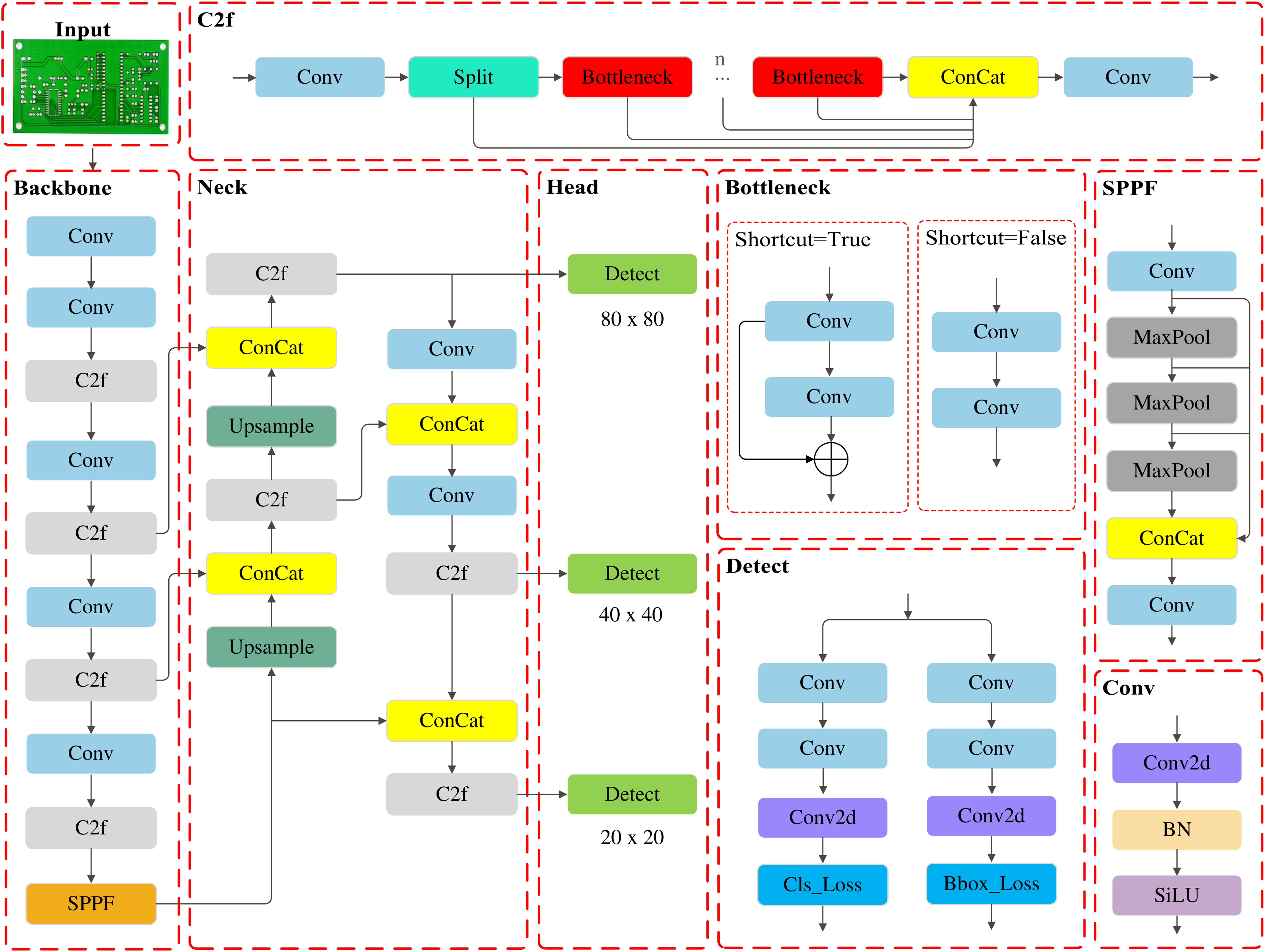
YOLOv8 is a widely utilized algorithm in the YOLO (Terven, Córdova-Esparza & Romero-González, 2023) series for tasks such as object detection, image classification, and instance segmentation, following the success of YOLOv5. Based on the model scaling factor, YOLOv8 offers five versions: n, s, m, l, and x. This article focuses on the lightweight YOLOv8n to meet the demands of resource-constrained environments. The architecture of the YOLOv8n algorithm is illustrated in Fig. 1.
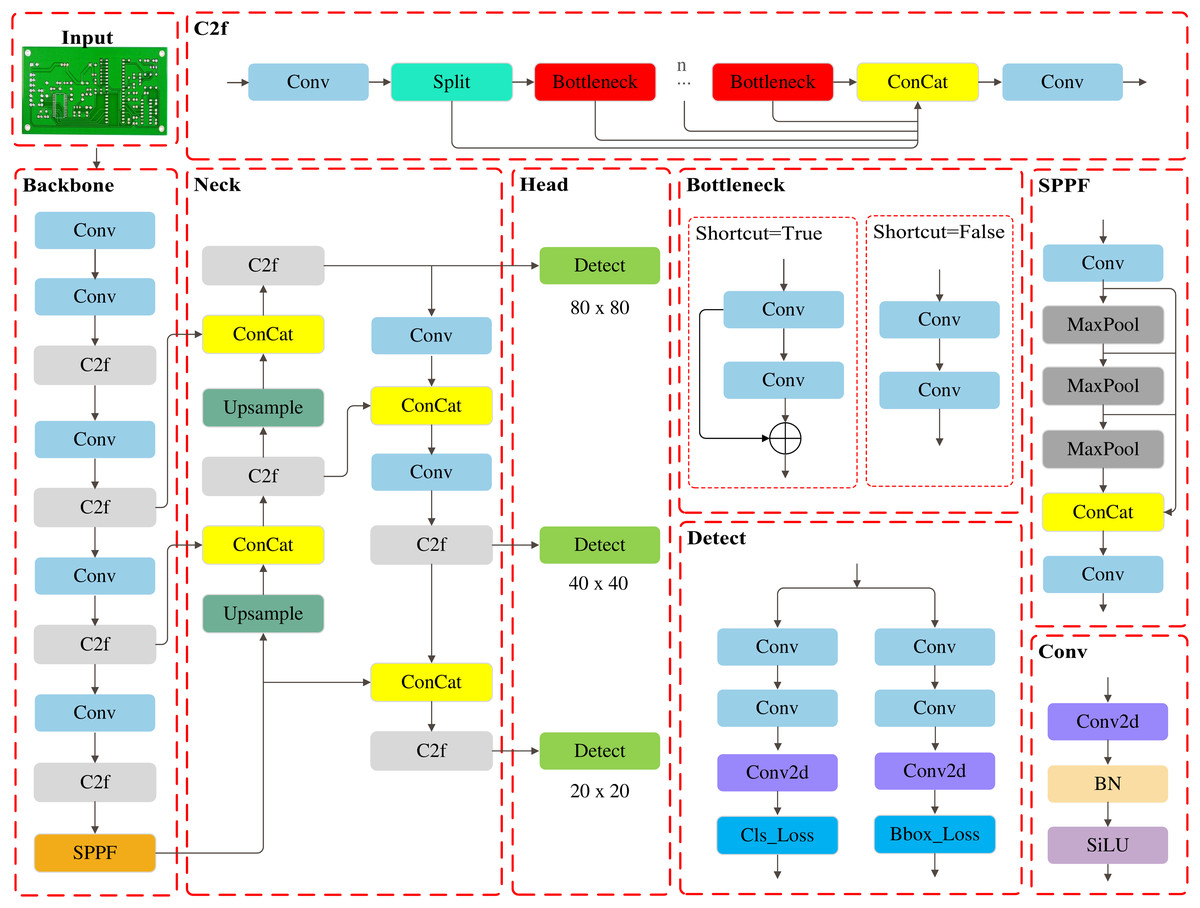
Figure 1: The architecture of the YOLOv8n algorithm.
The YOLOv8n consists of a backbone, neck, and head network. The backbone network is responsible for extracting deep features from images, employing the C2f module in place of the C3 module used in YOLOv5, while retaining the SPPF structure to expand the receptive field, thereby enhancing the detection capability for small objects. The neck network employs PAN-FPN for multiscale feature fusion, which significantly enhances detection robustness and stability while improving adaptability to complex scenes and diverse targets. The head network adopts a decoupled structure, handling anchor box regression and object classification tasks separately to ensure independent optimization of classification and localization.
Although YOLOv8n offers high accuracy with low computational cost, its real-time performance remains limited in resource-constrained scenarios, making further reduction in complexity and resource consumption a key optimization challenge.
Materials and Methods
Improvements to the YOLOv8 algorithm
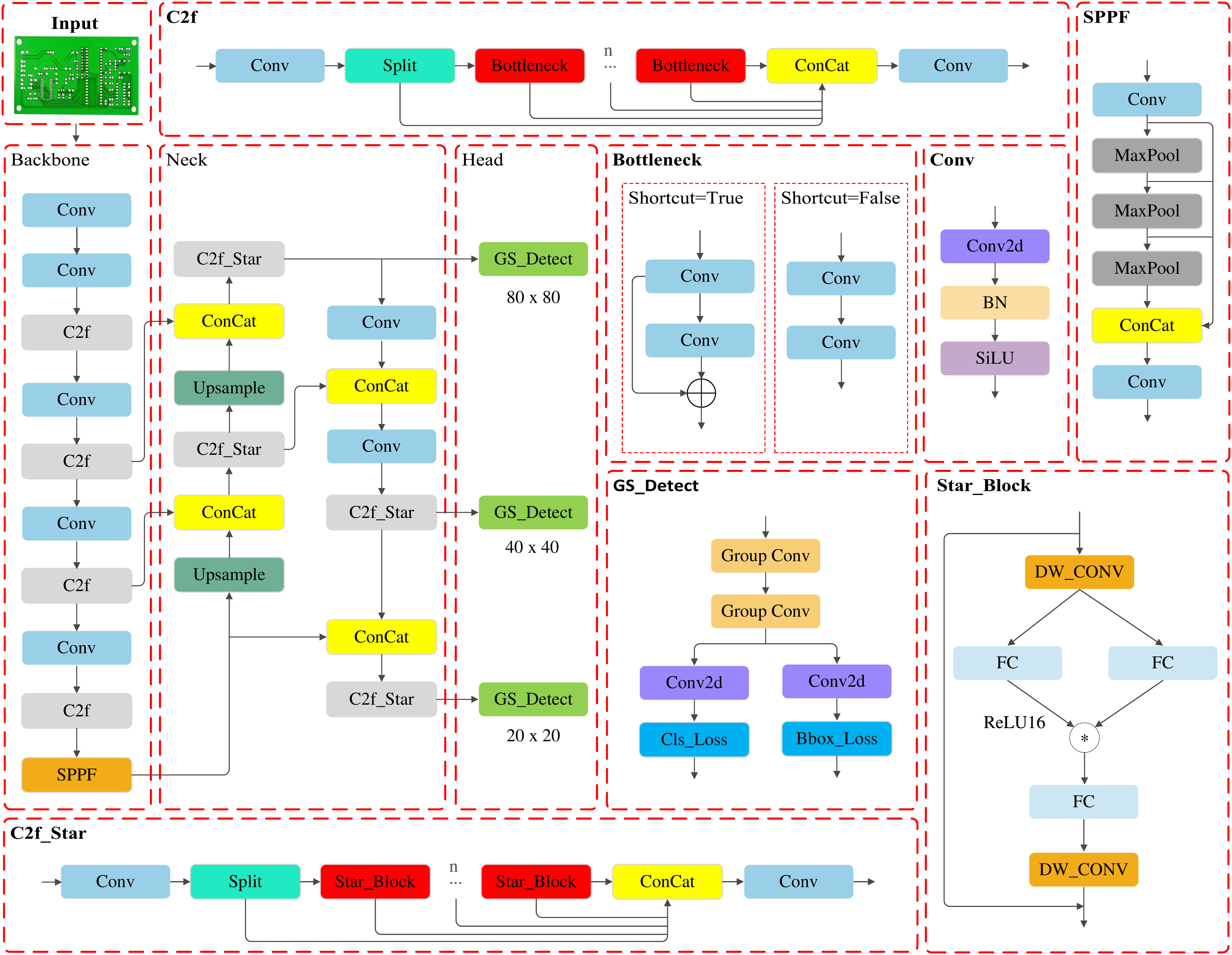
To address real-time and lightweight requirements for PCB industrial inspection, this article proposes an improved YOLOv8n model. As illustrated in Fig. 2, the modified architecture integrates:
-
(a)
Synergistic optimization of C2f_Star and GS_Detect: These components work together to reduce model complexity while enhancing detection efficiency.
-
(b)
Inner-MPDIoU loss replacing CIoU (Zheng et al., 2021): Significantly improves small-object localization accuracy, compensates for precision loss due to lightweighting, and accelerates convergence.
-
(c)
LAMP pruning strategy: Achieves maximum compression of parameters (Params) and computations (FLOPs) without accuracy degradation through threshold-controlled pruning.
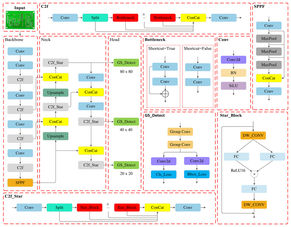
Figure 2: The improved structure of YOLOv8n.
This solution achieves an optimal accuracy-complexity-real-time balance for industrial-grade deployment.
C2f_Star module
In the Neck network of YOLOv8n, the feature extraction unit of the C2f module (Bottleneck) relies on element-wise summation to achieve feature fusion. While computationally efficient, this approach is limited in its ability to perform high-dimensional feature mapping and cross-channel interaction, resulting in insufficient representational capacity of the fused features. The original C2f module primarily performs linear addition of features at the same spatial location during fusion, lacking deep cross-channel interactions and nonlinear combinations. Consequently, enhancing feature representation often requires increasing network depth, which significantly raises both the number of parameters and computational cost.
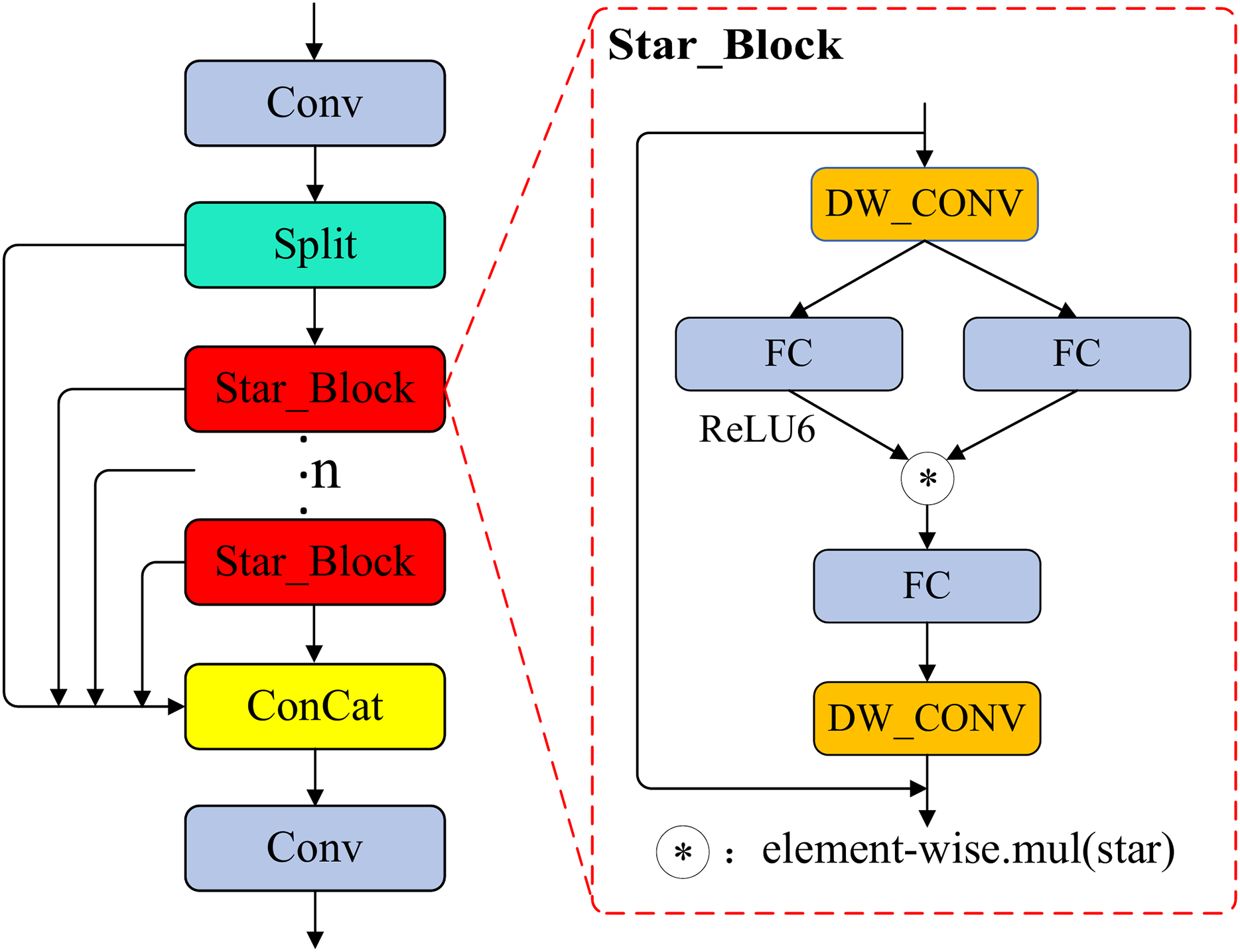
To address this limitation, we propose the improved C2f_Star module, illustrated in Fig. 3, which replaces the original Bottleneck unit with a lightweight Star_Block (Ma et al., 2024) unit. This module integrates the element-wise “Star” operation with depthwise separable convolutions, thereby enhancing feature interaction at the fusion stage. The “Star” operation performs element-wise multiplication between two branch features, preserving the original information while introducing pairwise nonlinear interactions that implicitly achieve high-dimensional feature mapping. The ‘Star’ operation can be represented by Eqs. (1)–(3): For an input of dimension d, the output feature dimension of this operation reaches , approximately , significantly expanding the feature representation space. This fusion approach introduces rich cross-channel correlations and feature diversity within a single fusion stage, allowing shallow local details and deep global semantic information to interact fully. As a result, it substantially enhances the depth and breadth of feature fusion without the need to increase network depth.
(1)
(2)
(3)
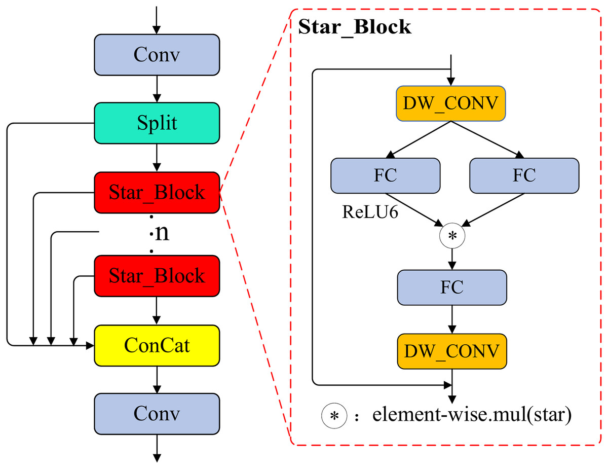
Figure 3: The structure of the C2f_Star module.
Depthwise separable convolution (Howard et al., 2017) decomposes standard convolution into two sequential stages: first, a depthwise convolution is applied independently to each channel of the input feature map; second, a pointwise convolution (1 × 1) fuses cross-channel information. The overall structure is illustrated in Fig. 4. In Star_Block, this structure is applied both before and after the “Star” fusion: the input first passes through a 7 × 7 depthwise separable convolution for spatial feature extraction, reducing computational load and strengthening spatial structure information; after fusion, a second 7 × 7 depthwise separable convolution further enhances the spatial representation of the fused features.
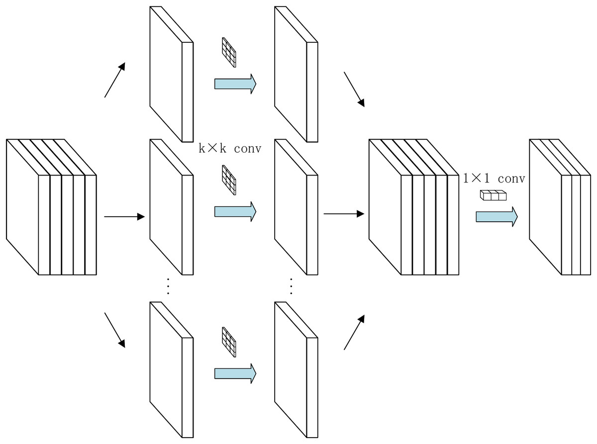
Figure 4: The structure of the DWConv module.
Specifically, as shown in Fig. 3, the input features of Star_Block are first processed by the initial 7 × 7 depthwise separable convolution, then fed in parallel into a dual-branch weight generator. Two 1 × 1 convolutional layers expand the channel dimension by a factor of three, producing feature tensors and . is activated by ReLU6 and subsequently undergoes element-wise multiplication with , achieving implicit high-dimensional mapping and generating fused features. The fused features are then compressed back to the original channel dimension via a 1 × 1 convolution and further refined by a second 7 × 7 depthwise separable convolution. Finally, a residual connection sums the processed features with the original input, ensuring information flow integrity and stable gradient propagation.
During training, the rectified linear unit 6 (ReLU6) activation function enhances nonlinear representational capacity, and DropPath (Huang et al., 2016) regularization effectively mitigates overfitting. Benefiting from the high-dimensional nonlinear fusion introduced by the “Star” operation and the efficient spatial feature extraction of depthwise separable convolutions, C2f_Star significantly improves cross-scale and cross-channel feature fusion while maintaining a lightweight design. This achieves an efficient balance between parameter count, computational cost, and detection accuracy, providing a practical solution for object detection on resource-constrained platforms.
GS_Detect module
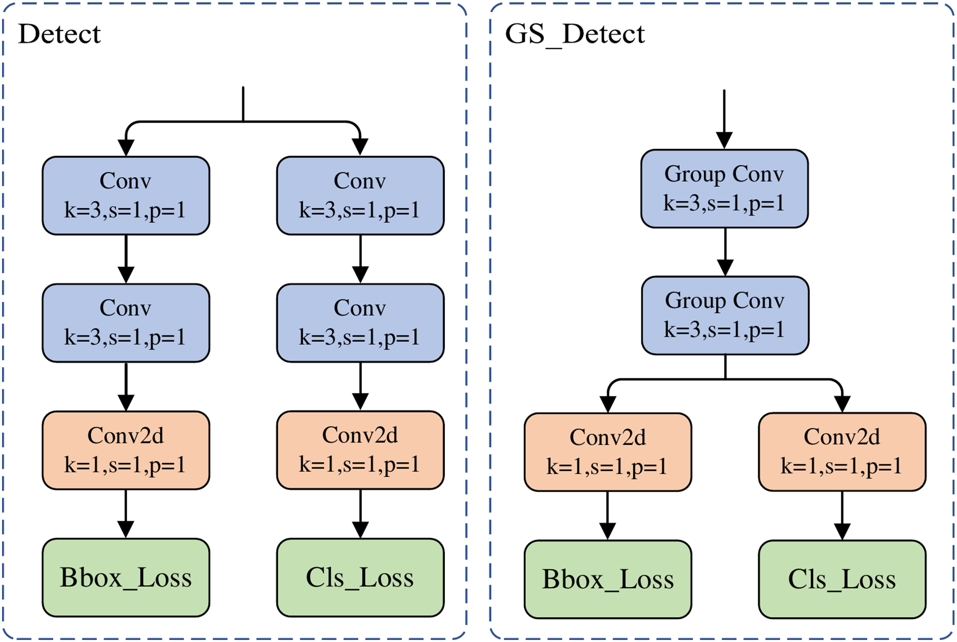
The decoupled detection head of YOLOv8n employs four separate 3 × 3 convolutional layers (two each for the classification and localization branches), resulting in excessively high network complexity, computational cost, and parameter count. To reduce complexity, this article proposes a lightweight detection head named GS_Detect. Its structure is shown in Fig. 5. Its core innovation lies in the integration of group convolution and a cross-task convolutional kernel sharing mechanism: it replaces the original four independent convolutional layers with two stages of weight-shared group convolutional layers. During the feature extraction stage, the classification and regression branches share the same set of convolutional kernels.
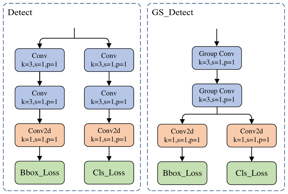
Figure 5: The structure of the GS_Detect module.
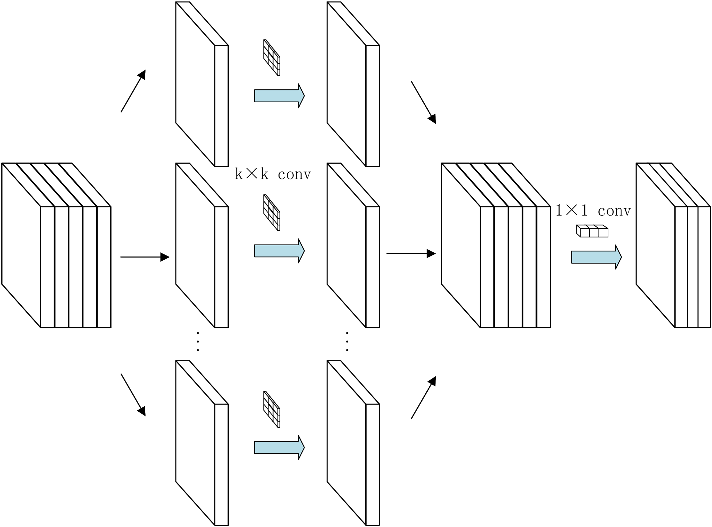
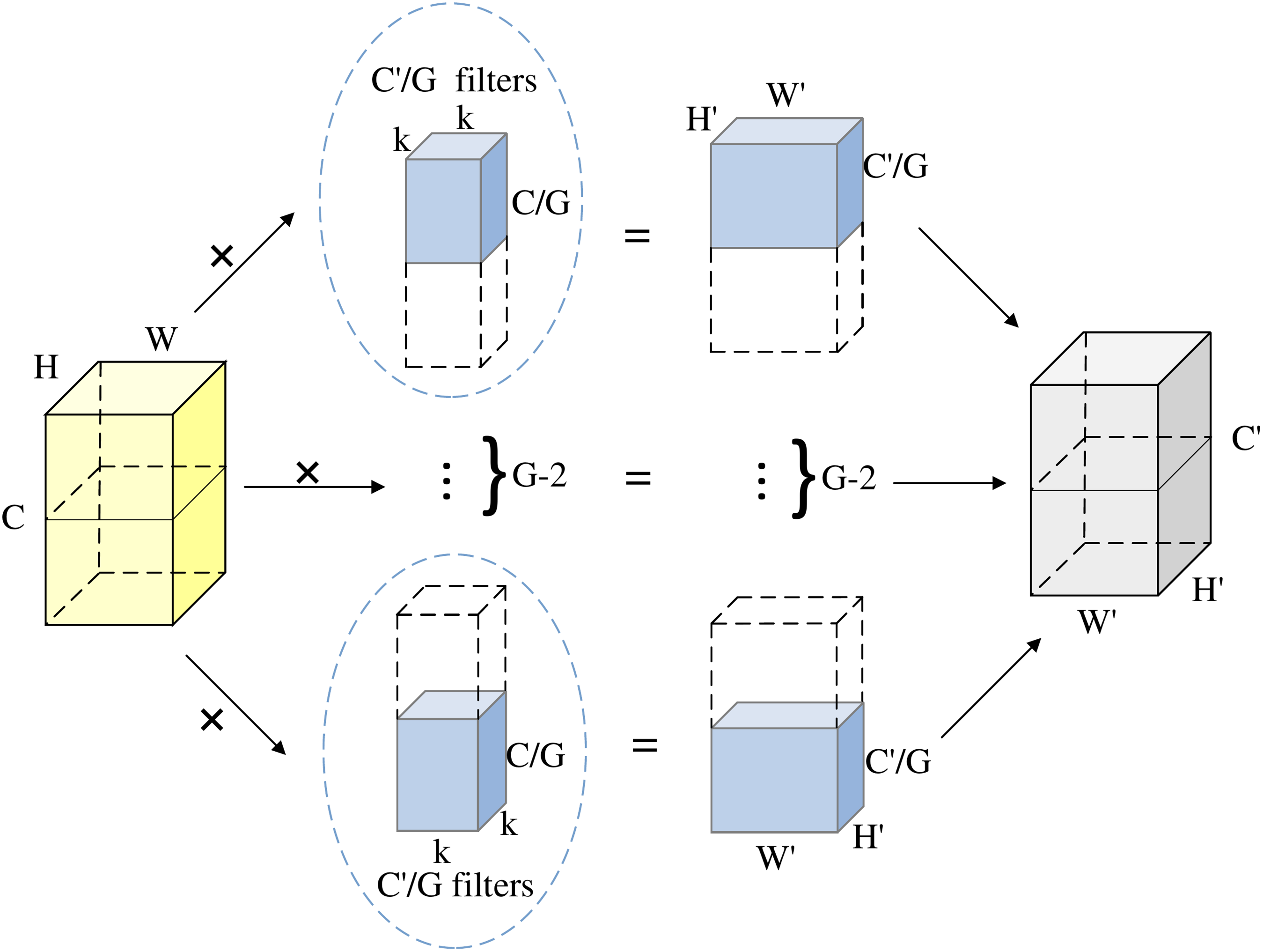
Group convolution divides the input feature map into groups, with each group undergoing convolution independently. This breaks the full connectivity redundancy inherent in standard convolution. As shown in Fig. 6, the input feature map with C channels is divided into G groups. Each group processes C/G input channels and produces C′/G output channels.:
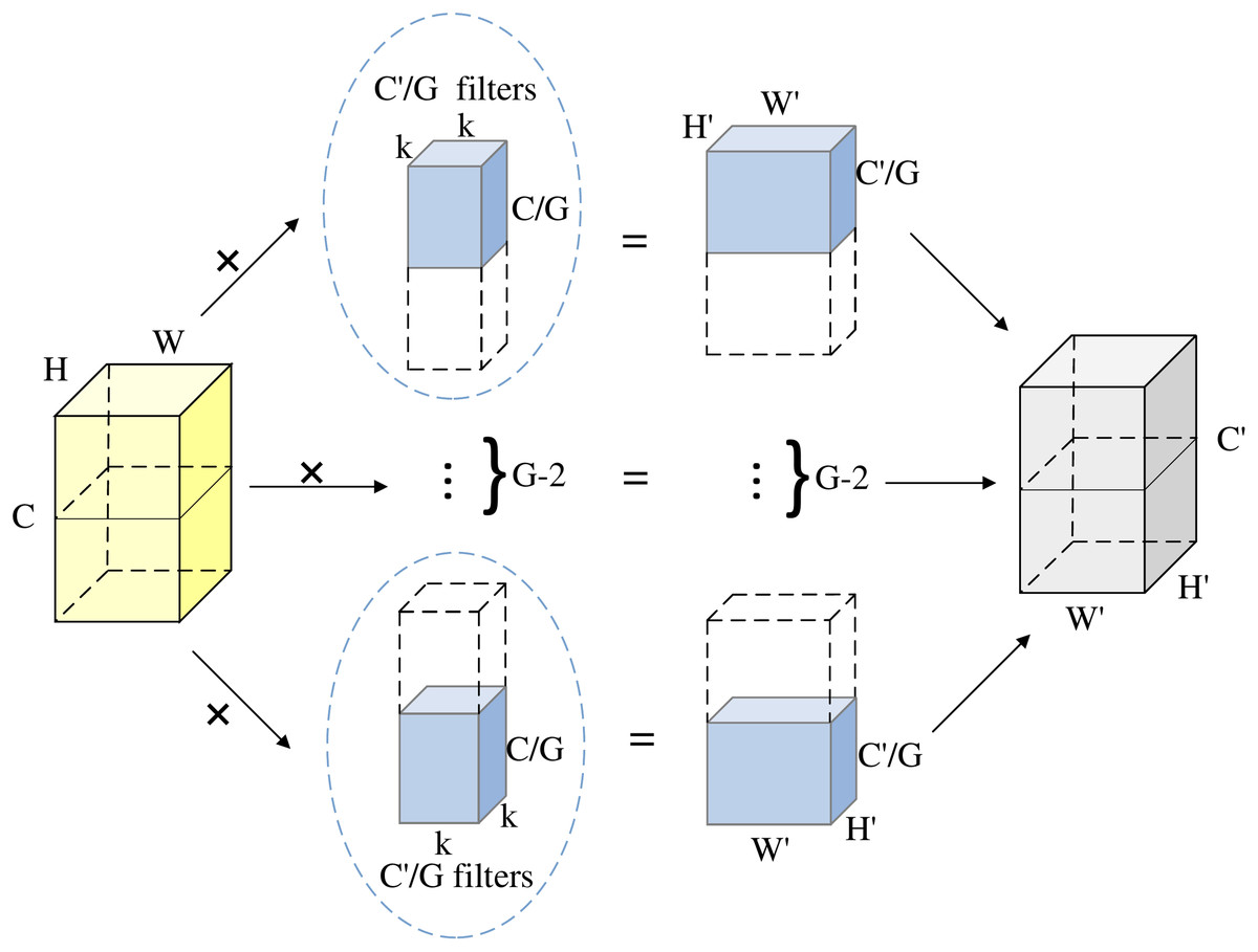
Figure 6: The structure of grouped convolution.
Parameter compression: Given input/output channel counts C and G, and a kernel size of , the theoretical compression ratio is G times.
Standard convolution parameter count:
(4)
Grouped convolution parameter count:
(5)
Computational efficiency: The decoupled structure between groups in grouped convolution reduces the parameter count to 1/G of standard convolution, with computational cost similarly reduced by a factor of G. By constraining the channel scope of convolution kernels, this design significantly enhances computational efficiency while maintaining feature representation capability.
The GS_Detect module adopts a hierarchical architecture to achieve decoupling and lightweighting of the detection task. Its structure, illustrated in Fig. 5, operates as follows: The input features are first processed by two stages of group convolution (G = 16). The key innovation lies in the full weight sharing of these two stages of group convolution kernels between the classification and regression branches, thereby eliminating the computational redundancy inherent in traditional dual-branch structures. Subsequently, the data flow is decoupled into two parallel branches: the classification branch (Cls_Loss) performs object category identification, while the regression branch (Bbox_Loss) handles bounding box localization. A standard 1 × 1 convolutional layer is deployed at the end of each branch for cross-channel feature aggregation and dimensionality adjustment. Through the integration of group convolution and the cross-task weight sharing mechanism, the GS_Detect module effectively compresses the model parameter count and computational cost while preserving the original detection performance, significantly enhancing deployment efficiency. Experiments validate that this module achieves substantial lightweighting while maintaining detection accuracy.
Inner-MPDIoU loss function
Bounding box regression accuracy is crucial for the localization performance of object detection. While the current YOLOv8n model employs the complete intersection over union (CIoU) loss (Zheng et al., 2021), it encounters limitations in PCB defect detection scenarios characterized by dense small objects. CIoU relies on constraints related to center point distance and aspect ratio, which tend to cause the model to overemphasize geometric alignment while neglecting the intrinsic characteristics of the defects. To address this limitation, this article proposes a hybrid loss function—Inner-MPDIoU. This loss integrates the design advantages of Inner-IoU (Zhang, Xu & Zhang, 2023) and Minimum Point Distance intersection over union (MPDIoU) (Ma & Xu, 2023), aiming to enhance the accuracy, robustness, convergence speed, and gradient stability of bounding box regression.
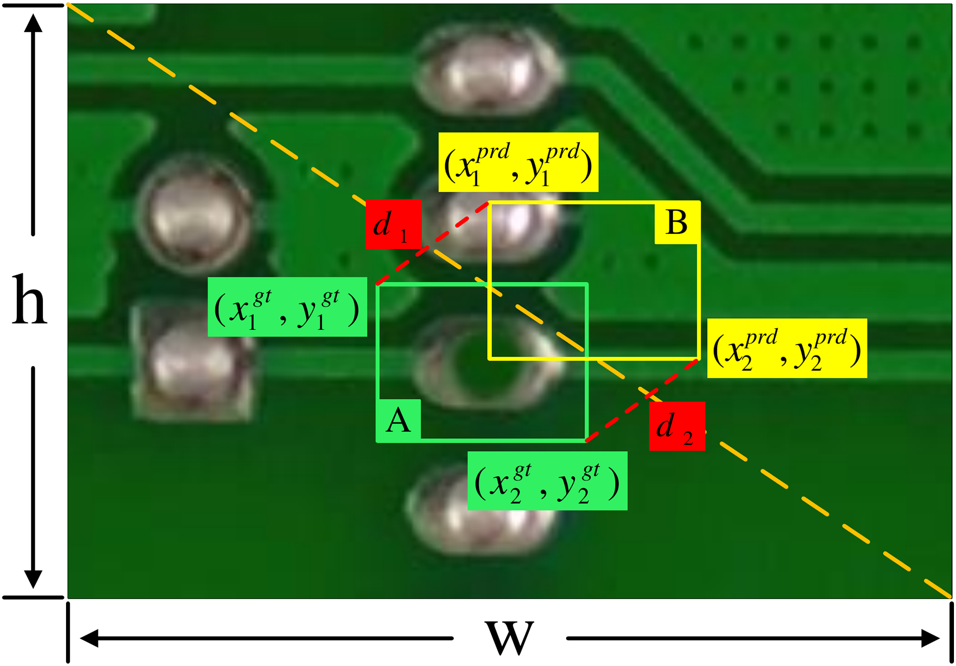
The core methodology of MPDIoU involves incorporating the minimum Euclidean distance between the four corner point coordinates of the predicted bounding box and the ground truth bounding box as a penalty term; its structure is depicted in Fig. 7. This mechanism effectively mitigates the sensitivity to errors exhibited by traditional CIoU for small and irregularly shaped objects. By focusing on boundary point alignment, it enhances regression precision, demonstrating significant effectiveness particularly when processing small and non-rectangular objects. Combined with Fig. 7, The MPDIoU optimization can be expressed by Eqs. (6)–(10):
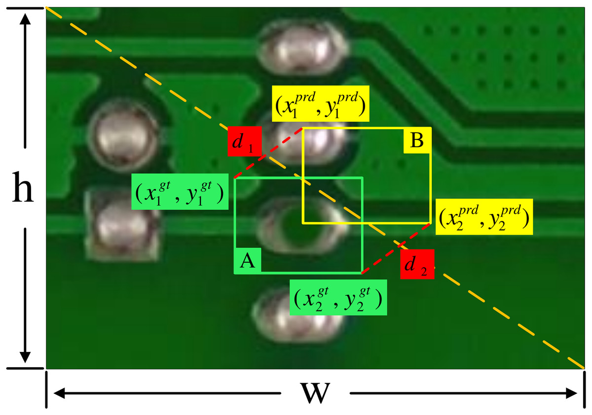
Figure 7: The structure diagram of the MPDIoU loss.
It first computes the fundamental intersection over union (IoU) between the predicted box B and ground truth box A as:
(6)
To incorporate geometric constraints, MPDIoU measures the squared Euclidean distances between the top-left corners :
(7) and bottom-right corners :
(8)
These distances are normalized by the ground truth box’s diagonal scale to ensure scale invariance. The final MPDIoU metric combines IoU with the corner alignment penalties:
(9)
The MPDIoU loss function is then derived as:
(10)
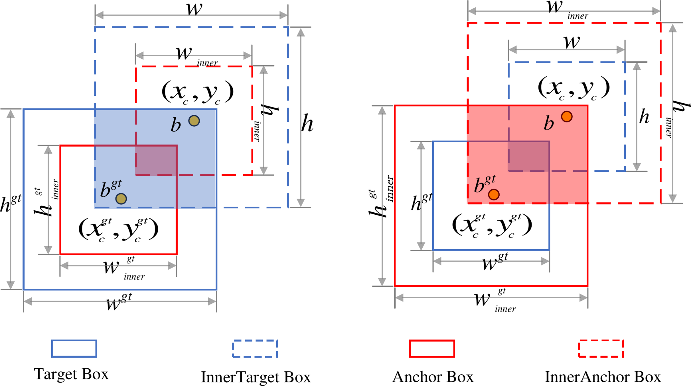
Inner-IoU constructs multi-scale auxiliary bounding boxes using scaling ratios (ratio) to impose nested constraints on ground truth and Anchor boxes. This enhances gradient strength for low-IoU samples, improving early-stage convergence speed and generalization capability. By incorporating multi-scale geometric priors, it strengthens the model’s understanding of object structures. The framework is shown in Fig. 8: Denoting the ground truth box as B and Anchor box as B, their center coordinates are and respectively. Widths and heights are , for GT and , for Anchor. The scaling factor ratio typically ranges from 0.5 to 1.5. The Inner-IoU calculation can be expressed by Eqs. (11)–(18).
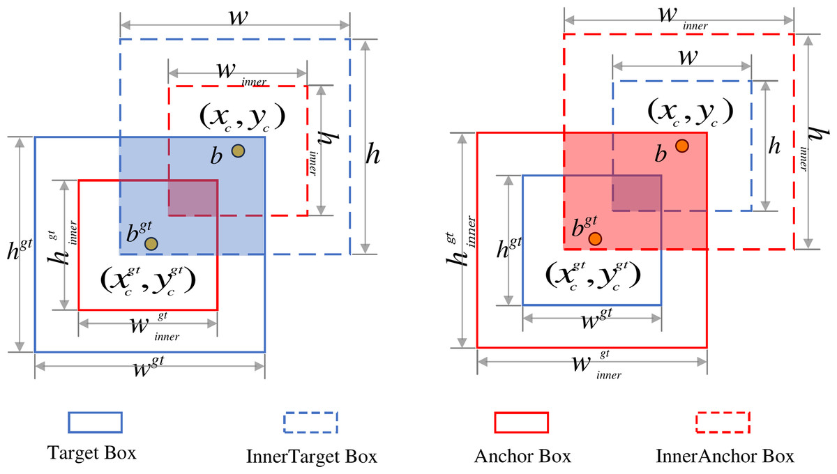
Figure 8: The structure of Inner-IoU loss.
Inner GT box boundaries:
(11)
(12) Inner anchor box boundaries:
(13)
(14) Intersection area:
(15) Union area:
(16) Inner-IoU loss:
(17)
(18)
The Inner-MPDIoU loss function organically combines the refined boundary-point alignment capability of MPDIoU with the multi-scale nested constraint advantages of Inner-IoU, thereby significantly improving bounding-box regression accuracy and training stability in dense small-object scenarios. Specifically, MPDIoU introduces the minimum Euclidean distance between the vertices of the predicted and ground-truth boxes as a penalty term, enabling more precise boundary alignment for tiny and irregularly shaped defects and effectively reducing regression errors caused by extremely small target sizes. Meanwhile, Inner-IoU leverages multi-scale auxiliary boxes to enhance the gradient signal for low-IoU samples, allowing the model to converge more rapidly in the early training stages while continuously improving localization accuracy for small objects. Compared with the CIoU loss used in the original model and several recently proposed losses (such as EIoU; Zhang et al., 2022, which focuses on optimizing width–height and center distance, and SIoU (Gevorgyan, 2022), which emphasizes angle and orientation matching), Inner-MPDIoU offers stronger characterization of boundary details and more stringent constraints on gradient stability, thereby achieving higher localization accuracy and convergence efficiency in small PCB defect detection. These advantages are corroborated by the loss experiments reported in this article. The computation process of Inner-MPDIoU is as follows:
(19)
LAMP model pruning
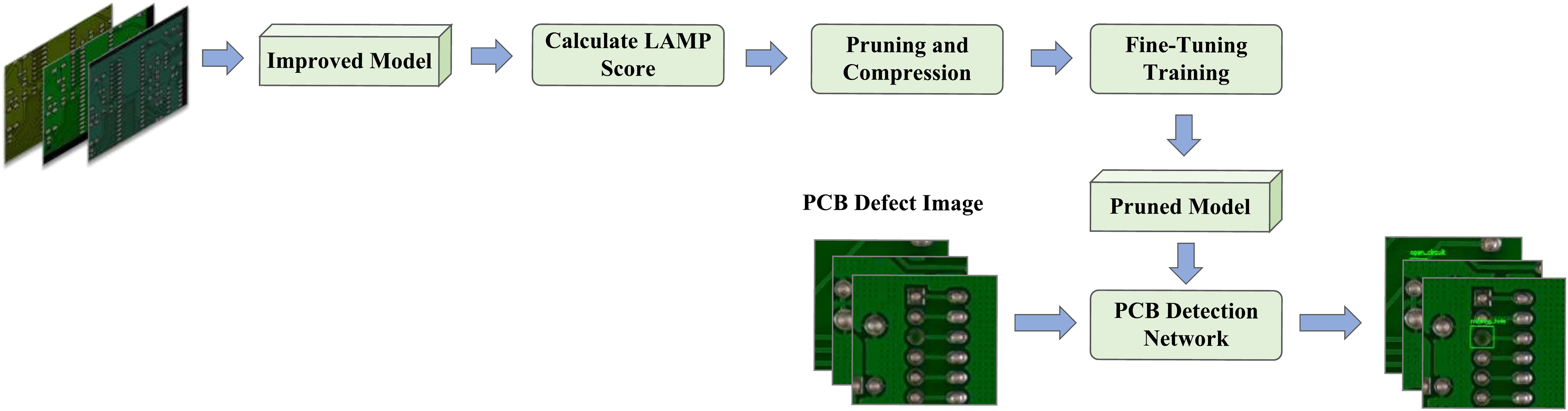
Despite reductions in parameter count and computational demands through lightweight optimizations, real-time industrial detection on resource-constrained devices remains challenging. This article applies LAMP-based channel pruning to refine the lightweight model, removing redundant connections while maintaining generalization and preventing overfitting. The pruning process is shown in Fig. 9.
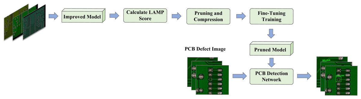
Figure 9: Model pruning flowchart.
LAMP adaptively prunes weights based on their absolute magnitudes without hyperparameter tuning or dependence on model architecture. It ranks weights in each layer and removes those below a set threshold, preserving network structure and effectiveness. This prevents excessive pruning in critical layers, as defined in Eq. (20).
(20)
In Eq. (20), signifies the LAMP score for the weight indexed by u, where W denotes the weights of the convolutional kernel represented as a one-dimensional vector. Here, u and v indicate indices, and the weights are organized in ascending order such that when u < v.
During the LAMP pruning experiments conducted on the lightweight YOLOv8n model, it was observed that pruning the already lightweight head network significantly reduced detection accuracy. Consequently, this portion was excluded from the pruning process. Post-pruning, both the model’s parameter count and computational load were reduced to half of that of the unpruned model, while detection accuracy improved by 0.7%. The experimental results indicate that LAMP pruning holds substantial application value in lightweight PCB defect detection and provides robust support for the widespread implementation of PCB defect detection technologies in industrial production.
Data preprocessing
To mitigate the risk of overfitting arising from the limited sample size in the PKU-Market-PCB dataset and to enhance the model’s generalization capability, this study conducted comprehensive data augmentation on the original dataset. All data processing methods described below were applied probabilistically to prevent excessive distortion or information redundancy caused by concurrent operations.
Mild affine transformations were applied. These included horizontal and vertical translation up to a maximum of 10% of the image dimensions, random scaling within the range [0.9, 1.1], and random shearing within the range [−5°, 5°]. These geometric transformations enhance the model’s robustness against variations in target location, scale, and orientation.
To further simulate illumination variations and color distribution differences encountered in practical applications, a color perturbation strategy was employed. This involved random adjustments to brightness, contrast, and saturation within ±20% of their original values, and random adjustments to hue within ±0.1. Additionally, each image had a 20% probability of being converted to grayscale to improve the model’s adaptability to variations in color space.
Finally, all images were converted into tensor format and normalized along the channel dimension: each pixel value was subtracted by 0.5 and then divided by 0.5, mapping the values to the range [−1, 1]. To prevent data leakage and ensure the objectivity of model evaluation, all augmentation operations were applied exclusively to the pre-defined training subset. Through the aforementioned strategies, the original dataset comprising 693 images was expanded to 3,660 images, substantially enriching the training data and leading to a significant improvement in model performance.
Evaluation method
To comprehensively evaluate the effectiveness of the proposed method, both ablation and comparison experiments were conducted. The ablation study analyzes the contribution of each component and optimization strategy by gradually modifying the baseline model, while the comparison experiment evaluates the proposed method against state-of-the-art approaches on the same dataset. Multiple evaluation metrics are employed, including precision (P), recall (R), mean average precision ([email protected]), giga floating point operations (GFLOPs), number of parameters (Params), model size, and inference speed measured in frames per second (FPS).
Precision and recall assess prediction accuracy, defined as:
(21)
(22)
The mAP is the average precision (AP) across all classes:
(23)
Here, Tp, Fp, and Fn represent the number of true positives, false positives, and false negatives, respectively, and N denotes the total number of object classes. [email protected] primarily measures detection accuracy. GFLOPs and the number of parameters indicate computational complexity and model compactness, while model size reflects storage requirements. FPS evaluates inference efficiency, which is crucial for real-time applications. These metrics jointly provide a comprehensive assessment of the model in terms of accuracy, efficiency, and deployment feasibility.
Experiments and results
Experimental environment configuration
The configuration of the experimental environment is detailed in Table 1, featuring an input image dimension of 640 × 640 pixels. The initial learning rate is established at 0.01, utilizing stochastic gradient descent (SGD) as the chosen optimization algorithm. The training regimen encompasses 300 epochs, with the Mosaic augmentation technique deactivated during the last 30 iterations. The batch size for training is set to 16.
| Name | Parameters |
|---|---|
| Operating system | Windows10 |
| CPU | Intel(R) 12th Gen Intel(R) Core(TM) i5-12400F 2.50 GHz |
| GPU | NVIDIA GeForce RTX 3060, 12 GB |
| Language | Python3.8.19 |
| Framework | Pytorch1.13.1+CUDA11.7 |
Dataset
This experiment employs two benchmark datasets with distinct data characteristics PKU-Market-PCB (https://doi.org/10.6084/m9.figshare.29558492.v2) and DeepPCB (https://github.com/tangsanli5201/DeepPCB.git) to validate the generalization capability and robustness of models in diverse PCB defect detection tasks through a cross-domain evaluation strategy.
The PKU-Market-PCB dataset, developed by Peking University’s Intelligent Robotics Laboratory, comprises 693 high-precision industrial PCB images. It encompasses six typical manufacturing defects: missing_hole, mouse_bite, open, short, spur, and spurious_copper, with their distribution illustrated in Fig. 10. To ensure evaluation rigor, the dataset was partitioned using a stratified random sampling strategy into training, validation, and test sets at an 8:1:1 ratio, maintaining balanced defect category distributions across all subsets.
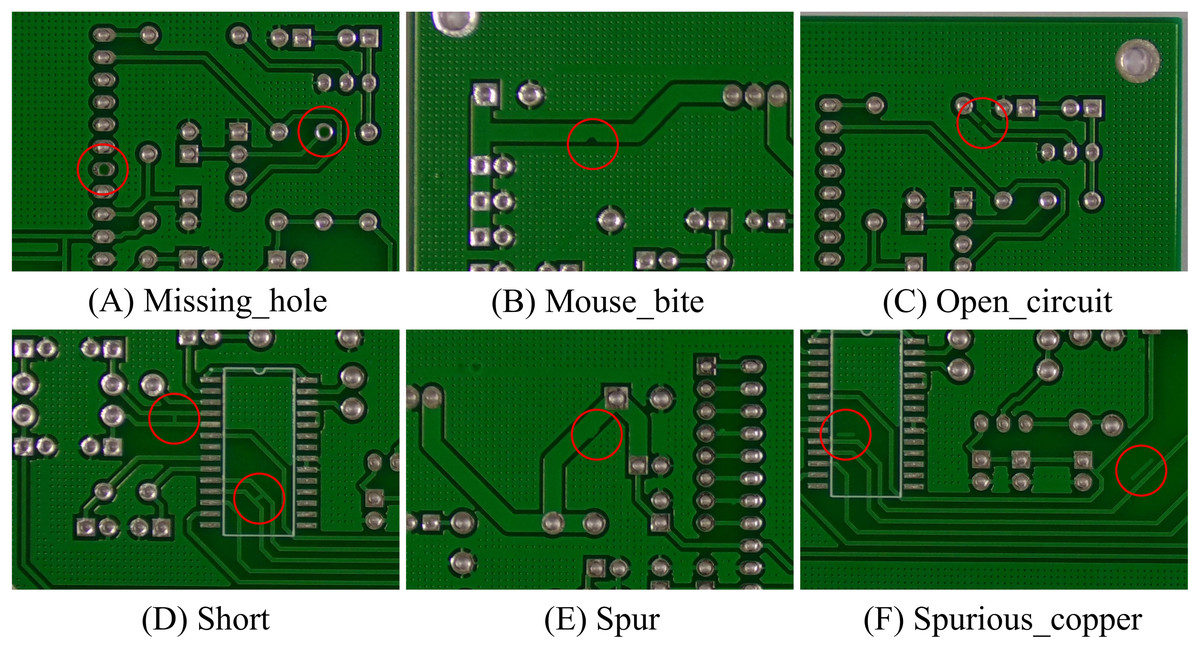
Figure 10: PCB category diagram.
The six types of defects in the PKU-Market-PCB dataset, including (A) Missing_hole, (B) Mouse_bite, (C) Open_circuit, (D) Short, (E) Spur, and (F) Spurious_copper.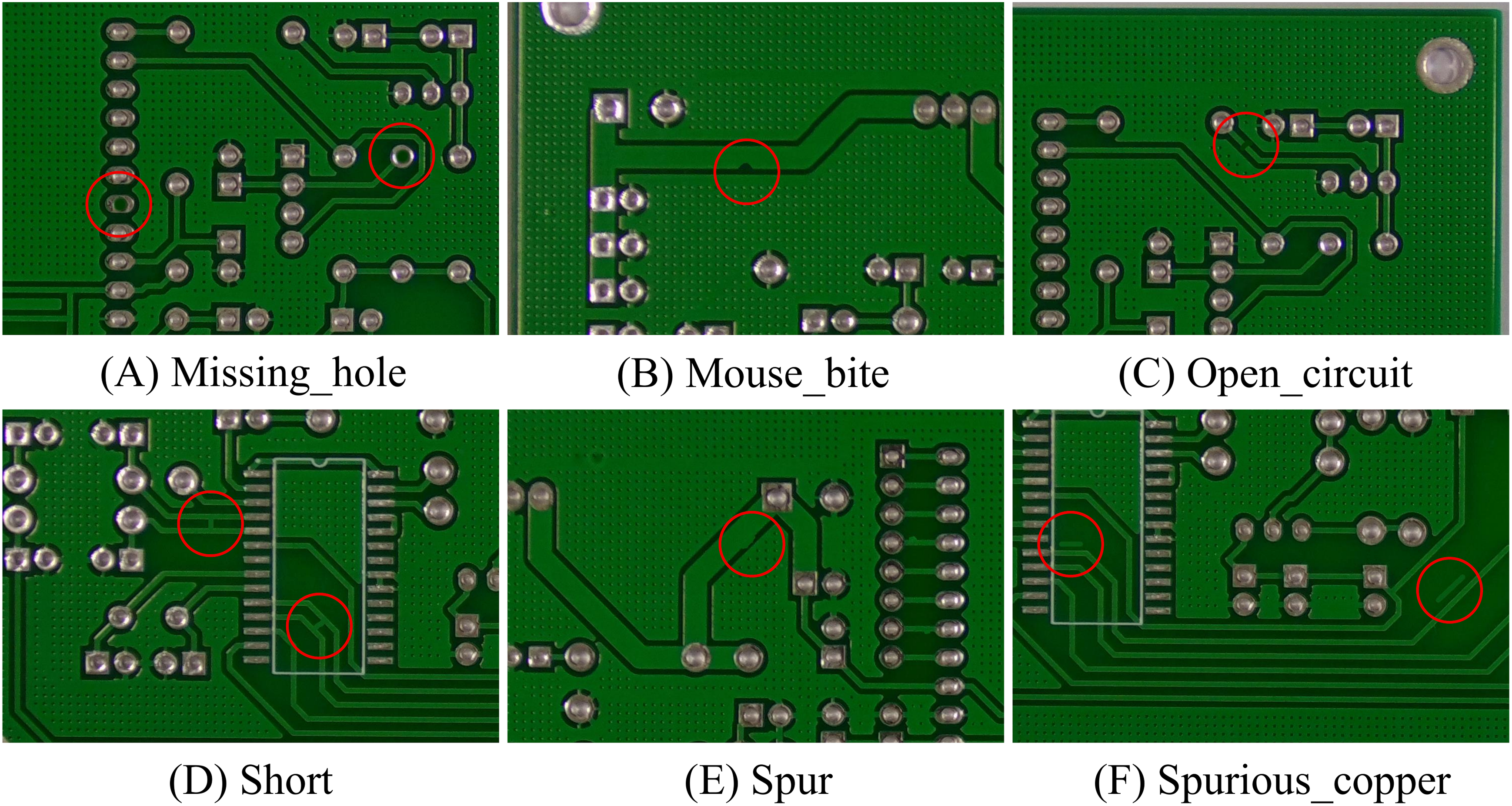
The DeepPCB dataset, constructed by Tang et al. (2019) using industrial-grade linear scanning CCD systems, contains 1,500 high-resolution PCB images (640 × 640 pixels). This dataset covers six defect categories: open, short, mousebite, spur, copper, and pin-hole. Each image contains 3–12 defect instances, with a spatial resolution of 48 pixels per millimeter (px/mm) to precisely capture microscopic defect morphological features. For data partitioning, this study strictly adheres to the same 8:1:1 ratio as PKU-Market-PCB, dividing the dataset into training, validation, and test sets.
Loss function experiment
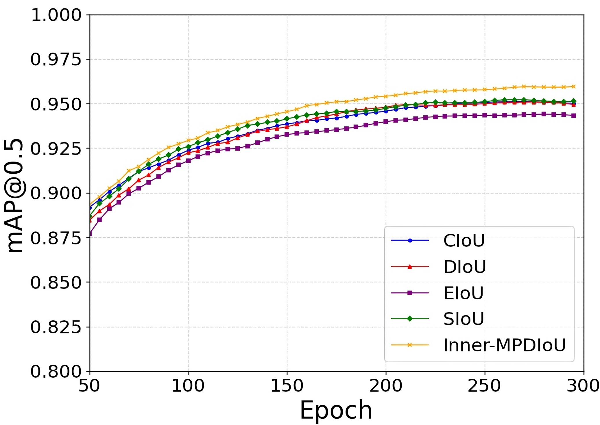
To evaluate the performance advantages of the proposed Inner-MPDIoU loss function in PCB defect detection tasks, this study conducts comparative experiments on the YOLOv8n architecture against mainstream loss functions including CIoU (Zheng et al., 2021), DIoU (Zheng et al., 2020), EIoU (Zhang et al., 2022), and SIoU (Gevorgyan, 2022). Experimental results demonstrate that Inner-MPDIoU significantly enhances detection accuracy, achieving a 1.3% improvement in [email protected] over CIoU. As illustrated in Fig. 11, the proposed loss function exhibits faster convergence speed and superior stability during training, with its performance curve consistently outperforming all baselines. These findings validate the effectiveness and superiority of Inner-MPDIoU in PCB defect detection scenarios.
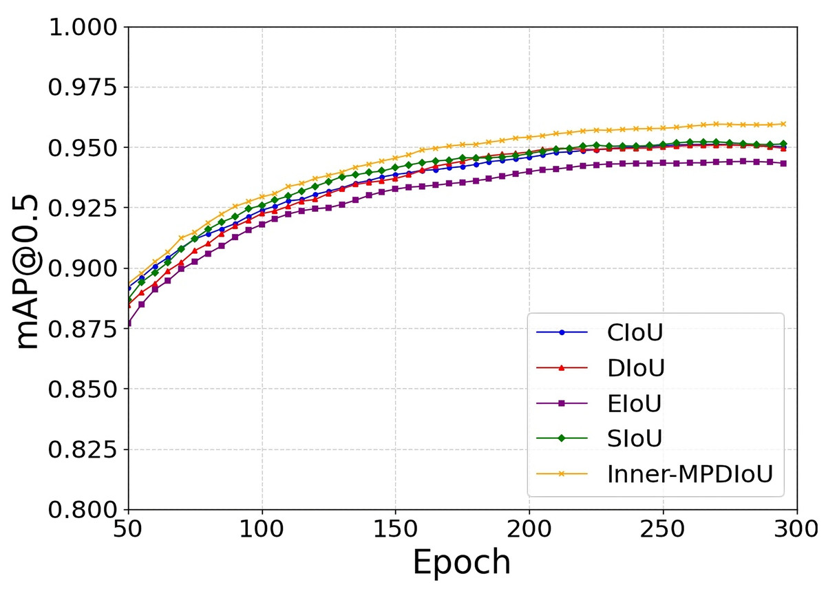
Figure 11: Loss curves during training.
Ablation experiments
Considering the prevalence of small-sized defect targets in the PCB dataset, the experimental Ratio parameter range was set to [1.1, 1.5]. Ablation experiments were conducted on the augmented PKU-Market-PCB dataset to evaluate the impact of different Ratio values on the Inner-MPDIoU loss function. As shown in Table 2, the model achieved optimal performance at Ratio = 1.3.
| Ratio [1.1, 1.5] | Precision/% | Recall/% | [email protected]/% |
|---|---|---|---|
| 1.1 | 97.4 | 92.1 | 96.0 |
| 1.2 | 97.9 | 92.2 | 96.0 |
| 1.3 | 97.1 | 92.3 | 96.3 |
| 1.4 | 97.6 | 91.6 | 95.9 |
| 1.5 | 97.7 | 91.5 | 95.7 |
To further verify the specific impact of different enhancement modules on model performance, a series of systematic ablation experiments were performed on the augmented PKU-Market-PCB dataset. Modules were incrementally integrated, with evaluation metrics including parameter count, computational cost, model size, and [email protected]. Results are summarized in Table 3.
| Dataset | Model | Inner-MPDIoU | C2f_Star | GS_Detect | LAMP | [email protected]/% | Params/M | GFLOPs/G | Model size/MB |
|---|---|---|---|---|---|---|---|---|---|
| PKU-Market-PCB | YOLOv8n | 95.0 | 3.01 | 8.1 | 6.3 | ||||
| I | √ | 96.3 | 3.01 | 8.1 | 6.3 | ||||
| II | √ | 95.1 | 2.71 | 7.2 | 5.7 | ||||
| III | √ | 94.5 | 2.42 | 5.6 | 5.1 | ||||
| IV | √ | √ | 95.8 | 2.71 | 7.2 | 5.7 | |||
| V | √ | √ | 95.4 | 2.42 | 5.6 | 5.1 | |||
| VI | √ | √ | 94.4 | 2.22 | 5.3 | 4.7 | |||
| VII | √ | √ | √ | 96.0 | 2.22 | 5.3 | 4.7 | ||
| VIII | √ | √ | √ | √ | 96.7 | 1.20 | 4.0 | 2.5 | |
| Deep-PCB | YOLOv8n | 98.6 | 3.01 | 8.1 | 6.3 | ||||
| I | √ | 98.8 | 3.01 | 8.1 | 6.3 | ||||
| II | √ | 97.9 | 2.71 | 7.2 | 5.7 | ||||
| III | √ | 98.0 | 2.42 | 5.6 | 5.1 | ||||
| IV | √ | √ | 98.8 | 2.71 | 7.2 | 5.7 | |||
| V | √ | √ | 98.1 | 2.42 | 5.6 | 5.1 | |||
| VI | √ | √ | 98.2 | 2.22 | 5.3 | 4.7 | |||
| VII | √ | √ | √ | 98.6 | 2.22 | 5.3 | 4.7 | ||
| VIII | √ | √ | √ | √ | 98.9 | 1.20 | 4.0 | 2.5 |
Model I, II, and III introduced the Inner-MPDIoU loss function, C2f_Star module, and GS_Detect detection head into the original YOLOv8n architecture, respectively. Results indicate that Model I increased [email protected] by 1.1% while maintaining model complexity; Model II significantly reduced model complexity with stable detection accuracy after incorporating C2f_Star; Model III slightly decreased detection accuracy but substantially reduced model complexity using GS_Detect, demonstrating high lightweight efficiency.
Models IV and V combined Inner-MPDIoU with either lightweight module, achieving both accuracy improvement and complexity reduction. Model VI integrated both lightweight modules, significantly compressing parameters, computation, and model size with a minor accuracy decline.
Model VII incorporated all three enhancement modules, improving detection performance while markedly reducing model complexity, demonstrating the feasibility of compensating for accuracy loss from lightweight modules via loss function optimization. Model VIII further introduced the LAMP pruning strategy, effectively eliminating redundant connections, mitigating overfitting, and significantly enhancing model compression efficiency.
As shown in Table 3, cross-dataset ablation experiments confirm that progressively adding enhancement modules yields consistent performance gains over YOLOv8n, validating module effectiveness while highlighting model generalizability and robustness.
Comparison experiments
To assess the improvements introduced by the YOLOv8n-based algorithm, we conducted comprehensive comparative experiments using the augmented PKU-Market-PCB dataset. The experimental framework incorporated traditional algorithms, lightweight models, and state-of-the-art object detection algorithms, including Faster-RCNN (Ren et al., 2016) SSD (Liu et al., 2016), RetinaNet (Lin et al., 2017), YOLOv3-tiny (Redmon & Farhadi, 2018),EfficientDet (Tan, Pang & Le, 2020), YOLOv5n, YOLOv5s, YOLOX-tiny (Ge et al., 2021), YOLOv6 (Li et al., 2022), YOLOv7-tiny (Wang, Bochkovskiy & Liao, 2023), YOLOv8n with MobileNetV4 (Qin et al., 2024) backbone, the YOLOv8 series, RT-DETR (Zhao et al., 2024), YOLOv9-t (Wang, Yeh & Mark Liao, 2024), and YOLOv10-n (Wang et al., 2024). Detailed results from these experiments are presented in Table 4.
| Dataset | Model | Params/M | GFLOPs/G | Size/MB | [email protected]/% | FPS/S |
|---|---|---|---|---|---|---|
| PKU-Market-PCB | Faster-RCNN | 41.4 | 134 | 318 | 92.0 | 17 |
| SSD | 26.3 | 62.7 | 96.1 | 85.5 | 36 | |
| RetinaNet | 19.9 | 98 | 159 | 84.3 | 24 | |
| YOLOv3-tiny | 12.1 | 18.9 | 24.4 | 86.0 | 147 | |
| DifficientDet | 3.9 | 22.6 | 17.1 | 89.4 | 34 | |
| YOLOv5n | 2.5 | 7.1 | 5.3 | 95.0 | 76 | |
| YOLOv5s | 7.02 | 15.8 | 14.5 | 97.3 | 66 | |
| YOLOX-tiny | 5.0 | 6.5 | 70 | 85.2 | 53 | |
| YOLOv6 | 4.2 | 11.8 | 8.7 | 93.5 | 78 | |
| YOLOv7-tiny | 6.0 | 13.2 | 12.3 | 83.0 | 72 | |
| YOLOv8n (Base) | 3.0 | 8.1 | 6.3 | 95.0 | 83 | |
| YOLOv8s | 11.1 | 28.4 | 22.5 | 97.4 | 75 | |
| YOLOv8m | 25.8 | 78.7 | 52 | 97.6 | 58 | |
| YOLOv8n (MobileNetV4) | 5.70 | 22.5 | 11.7 | 91.5 | 72 | |
| RT-DETR | 19.9 | 57 | 40 | 98.6 | 41 | |
| YOLOv9-t | 2.0 | 7.6 | 4.6 | 94.3 | 42 | |
| YOLOv10-n | 2.3 | 6.5 | 5.8 | 96.1 | 78 | |
| Our | 1.2 | 4.0 | 2.5 | 96.7 | 86 | |
| Deep-PCB | Faster-RCNN | 41.4 | 134 | 318 | 97.2 | 17 |
| SSD | 26.3 | 62.7 | 96.1 | 94.5 | 40 | |
| RetinaNet | 19.9 | 98 | 159 | 93.2 | 32 | |
| YOLOv3-tiny | 12.1 | 18.9 | 24.4 | 94.6 | 120 | |
| DifficientDet | 3.9 | 22.6 | 17.1 | 95.8 | 37 | |
| YOLOv5n | 2.5 | 7.1 | 5.3 | 98.0 | 85 | |
| YOLOv5s | 7.02 | 15.8 | 14.5 | 98.2 | 67 | |
| YOLOX-tiny | 5.0 | 6.5 | 70 | 93.4 | 63 | |
| YOLOv6 | 4.2 | 11.8 | 8.7 | 98.1 | 91 | |
| YOLOv7-tiny | 6.0 | 13.2 | 12.3 | 90.5 | 75 | |
| YOLOv8n (Base) | 3.0 | 8.1 | 6.3 | 98.6 | 86 | |
| YOLOv8s | 11.1 | 28.4 | 22.5 | 99.0 | 86 | |
| YOLOv8m | 25.8 | 78.7 | 52 | 99.0 | 49 | |
| YOLOv8n (MobileNetV4) | 5.70 | 22.5 | 11.7 | 95.4 | 71 | |
| RT-DETR | 19.9 | 57 | 40 | 98.5 | 52 | |
| YOLOv9-t | 2.0 | 7.6 | 4.6 | 98.7 | 46 | |
| YOLOv10-n | 2.3 | 6.5 | 5.8 | 98.5 | 80 | |
| Our | 1.2 | 4.0 | 2.5 | 98.9 | 86 |
The experiments showed that traditional detectors like Faster-RCNN, SSD, and RetinaNet had lower accuracy, high parameters, and large computational costs, leading to slow inference. For example, Faster-RCNN achieved 92.0% [email protected] but with 41.4M parameters and 134G FLOPs. In comparison, the proposed algorithm used only 1.2M parameters and 4.0G FLOPs, reached 86 FPS, and achieved 96.7% [email protected], significantly outperforming these models.
Although lightweight models improved efficiency, their accuracy remained limited. YOLOv3-tiny, YOLOX-tiny, and YOLOv7-tiny achieved [email protected] of 86.2%, 85.2%, and 83.0%, respectively. EfficientDet reached 89.4% [email protected] but only 34 FPS, unsuitable for real-time use. YOLOv8n with MobileNetV4 achieved 72 FPS but only 91.5% [email protected]. YOLOv5n and YOLOv6 attained higher accuracy (95.0% and 93.5%), yet still trailed the proposed method. YOLOv5s achieved 97.3% [email protected], but with substantially larger size and computation.
As the baseline, YOLOv8n balanced accuracy and complexity but was still outperformed by our model. Larger models like YOLOv8s and YOLOv8m reached 97.4% and 97.6% [email protected], but required 22.5M/28.4G and 52.0M/78.7G, respectively, making them impractical under resource constraints.
Among newer models, RT-DETR achieved 98.6% [email protected] but had 19.9M parameters and 40G FLOPs, with slow inference. YOLOv9-t and YOLOv10-n balanced accuracy and efficiency, achieving 94.3% and 96.1% [email protected] with 2.0M/42 FPS and 2.3M/78 FPS. Although YOLOv10-n was competitive, the proposed method offered a better balance.
In summary, our approach significantly reduces model complexity while maintaining high accuracy, outperforming most models. Additional experiments on the DeepPCB dataset (Table 4) confirmed that the algorithm preserves high accuracy, low complexity, and strong generalization across datasets, demonstrating robustness to noise and data distribution variations.
Discussion
To evaluate the detection performance of the proposed algorithm for six types of PCB defects, Gradient-weighted Class Activation Map (Grad-CAM) heatmaps of the original YOLOv8n and the improved model are first compared. Figure 12 displays their attention region distributions, with visual analysis revealing differences in detection mechanisms and feature extraction capabilities.
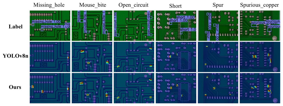
Figure 12: YOLOv8n vs. our method heatmap comparison.
Comparison of PCB defect detection results between the baseline model YOLOv8n and the improved model. The Grad-CAM heatmaps highlight the detected defect regions. Each column represents a different defect type, including missing holes, mouse bites, open circuits, shorts, spurs, and spurious copper.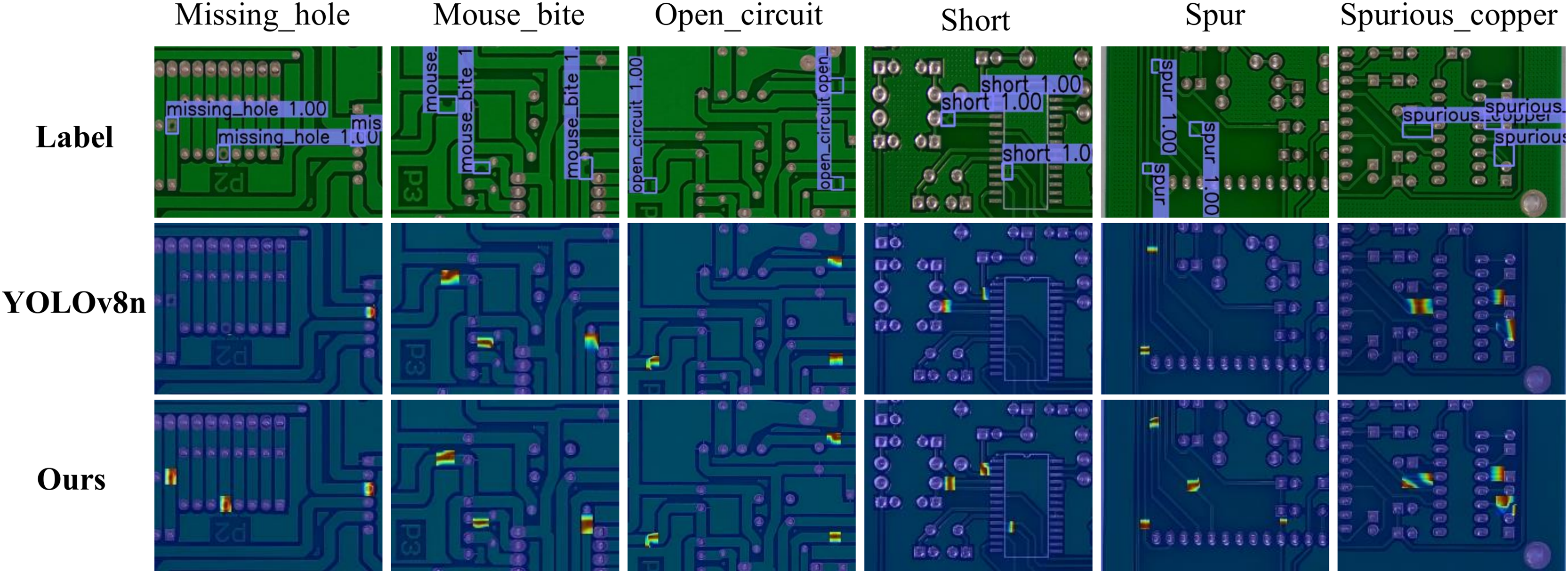
Comparative experiments further assess the performance and perception capabilities of YOLOv5n, YOLOv8n, RT-DETR, YOLOv10-n, and the proposed algorithm in PCB defect detection. Randomly sampled detection results in Figure 13 indicate: RT-DETR exhibits no missed or false detections; the proposed model shows only one missed detection in the “Spur” category; other algorithms exhibit missed detections for both “Open” and “Spur” defects. Although RT-DETR demonstrates superior detection accuracy, its complex structure incurs high computational costs and deployment difficulties, limiting industrial applications. In contrast, the proposed model achieves a better balance between accuracy and complexity, better aligning with industrial requirements emphasizing both efficiency and reliability.
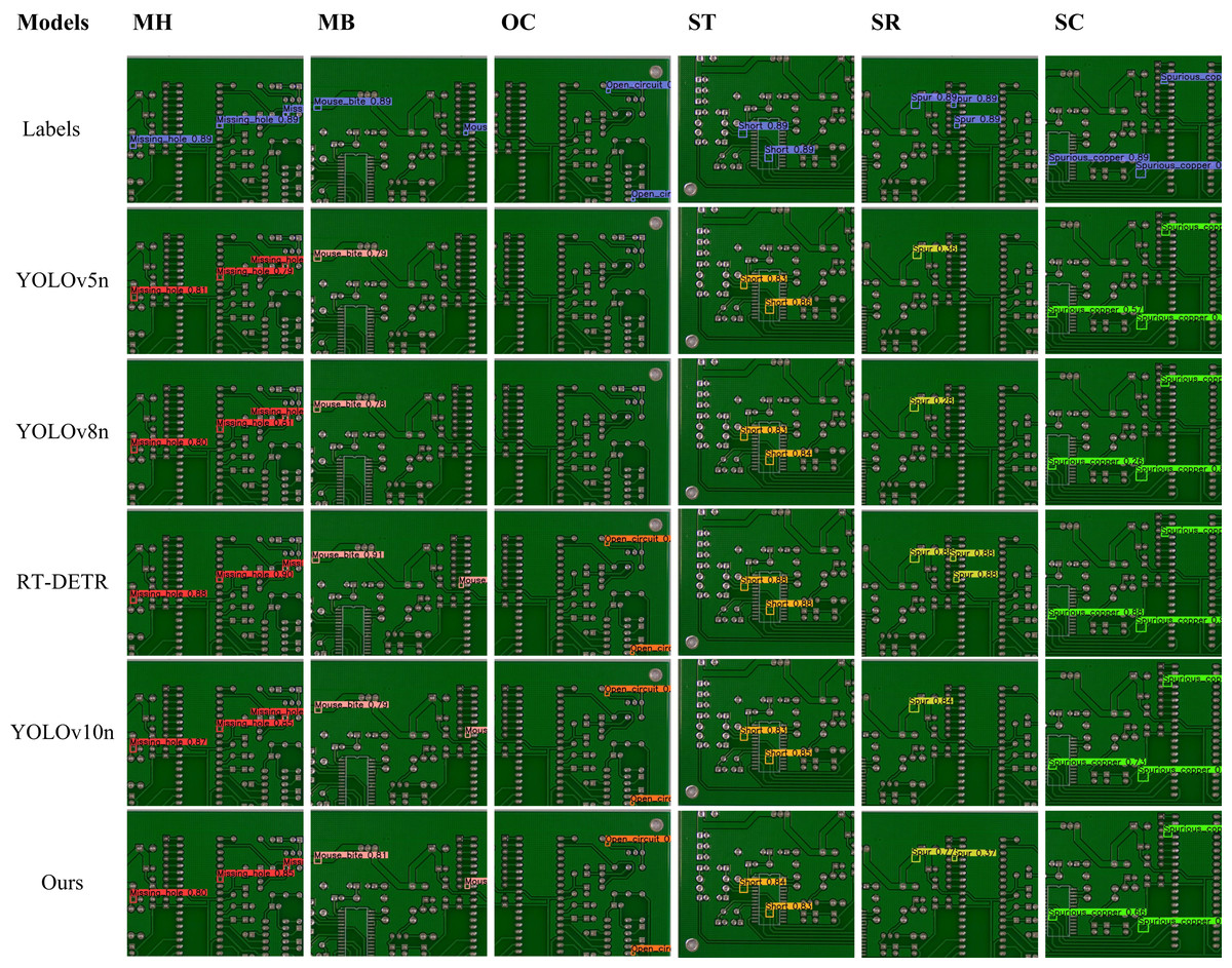
Figure 13: Visualization of experimental results.
This figure presents a comparative visualization of PCB defect detection results across different models. The first row denotes six defect types: missing holes (MH), mouse bites (MB), open circuits (OC), shorts (ST), spurs (SR), and spurious copper (SC). The first column lists the models evaluated, including YOLOv5n, YOLOv8n, RT-DETR, YOLOv10-n, and our proposed model. The “Labels” row provides the ground truth annotations for each defect type. Colored bounding boxes highlight the detected defect regions, allowing for a direct comparison of detection performance among the models.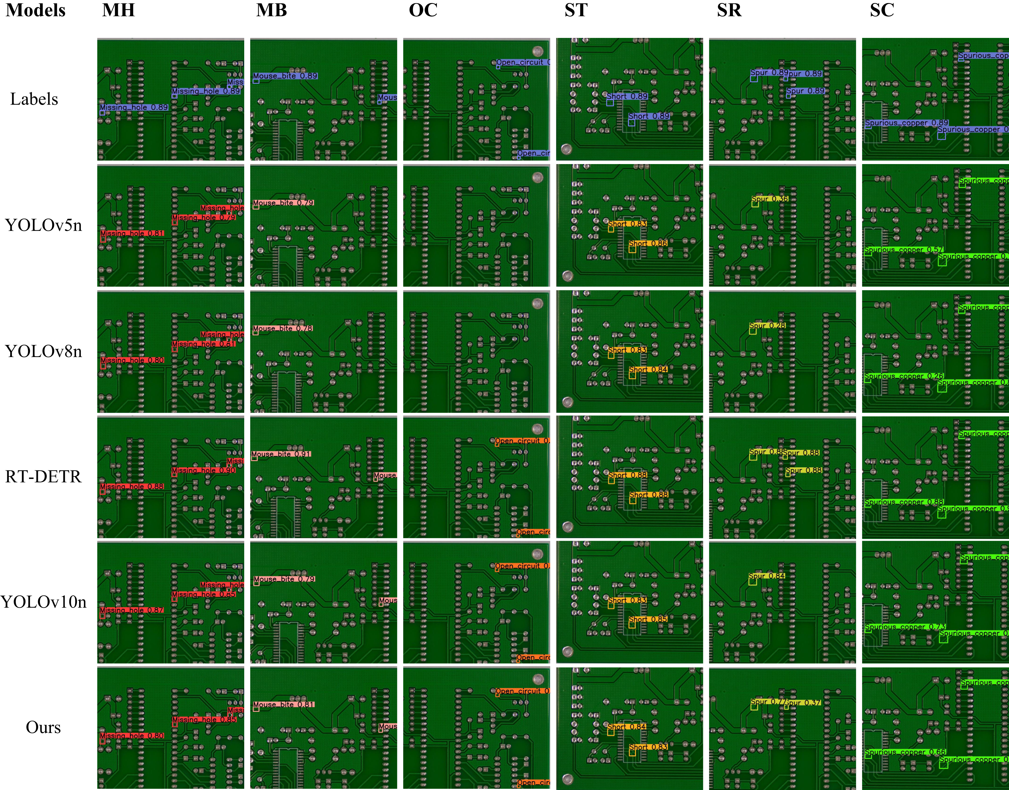
Although the proposed lightweight detection framework performs well in PCB defect detection, limitations remain requiring further refinement. First, detection performance remains suboptimal for extremely small or edge-blurred defects, particularly those with indistinct features or partial occlusion. Second, the model exhibits sensitivity to variations in image acquisition conditions (e.g., strong light interference, high noise, or motion blur), which are common in real industrial environments. Additionally, while the adopted pruning strategy significantly reduces parameter count and computational costs, it may compromise model robustness in complex or highly variable scenarios. Future work could explore more adaptive model compression methods or integrate multi-scale feature fusion strategies with lightweight convolutional modules to enhance stability and generalization in broader application environments.
Conclusions
To address the accuracy–complexity trade-off in PCB defect detection, this article proposes a lightweight improved YOLOv8n model. It enhances efficiency via a compact C2f_Star neck module, merging C2f and Star_Block structures. The GS_Detect head employs grouped convolution for further optimization, while the Inner-MPDIoU loss replaces CIoU, boosting localization accuracy—especially for PCB micro-defects. LAMP-structured pruning removes redundant connections, significantly reducing parameters and computational costs. On the augmented PKU-Market-PCB dataset, the improved model reduces parameters by 60%, computation by 51%, and size by 60%, while increasing accuracy from 95.0% to 96.7%. DeepPCB experiments validate its robustness and generalization. Although balancing accuracy and complexity well, challenges remain for extremely small/blurred-edge defects under complex imaging. Future work will enhance robustness via adaptive compression and stronger feature representation.