
TuFoC: regional classification of Turkish folk music recordings using deep learning on Mel spectrograms
- Published
- Accepted
- Received
- Academic Editor
- Rowayda Sadek
- Subject Areas
- Artificial Intelligence, Data Mining and Machine Learning, Neural Networks
- Keywords
- Deep learning, Music information retrieval, Regional classification, Mel spectrograms, Turkish folk music, Convolutional neural networks
- Copyright
- © 2025 Abidin
- Licence
- This is an open access article distributed under the terms of the Creative Commons Attribution License, which permits unrestricted use, distribution, reproduction and adaptation in any medium and for any purpose provided that it is properly attributed. For attribution, the original author(s), title, publication source (PeerJ Computer Science) and either DOI or URL of the article must be cited.
- Cite this article
- 2025. TuFoC: regional classification of Turkish folk music recordings using deep learning on Mel spectrograms. PeerJ Computer Science 11:e3233 https://doi.org/10.7717/peerj-cs.3233
Abstract
The regional classification of Turkish folk music remains a relatively unexplored domain in music information retrieval, particularly when leveraging raw audio signals for deep learning. This study addresses this gap by investigating how modern deep learning architectures can effectively classify regional folk recordings from limited original data using carefully designed spectrogram inputs. To address this challenge, we present Turkish Folk Music Classification (TuFoC), a deep learning-based approach that classifies Turkish folk music recordings according to their region of origin using Mel spectrogram representations. We investigate two complementary architectures: a MobileNetV2-based convolutional neural network (CNN) for extracting spatial representations, and a long short-term memory (LSTM) network for modeling temporal dynamics. To engage critically with the state of the art, we replicate a classical machine learning pipeline that combines histogram of oriented gradients (HOG) features with a Light Gradient-Boosting Machine (LightGBM) classifier and Synthetic Minority Oversampling Technique (SMOTE)-based oversampling. This baseline achieves competitive results, particularly on GAD, with 92.53% accuracy and macro F1-score. However, our CNN architecture not only marginally outperforms the baseline on the gently augmented dataset (GAD) (92.68% accuracy) but also demonstrates superior consistency across all dataset variants. While the LSTM model underperforms on original dataset (OD) and strongly augmented dataset (AD), it improves markedly on GAD, validating the importance of balanced data preparation. Experimental results, obtained through stratified 10-fold cross-validation repeated over 30 independent runs, demonstrate that the proposed CNN architecture delivers the highest and most stable classification performance. Beyond performance gains, our approach offers key advantages in generalization, scalability, and automation, as it bypasses the need for domain-specific feature design. The findings confirm that deep neural models trained on Mel spectrograms constitute a flexible and robust alternative to classical pipelines, holding promise for future applications in computational ethnomusicology and music information retrieval.
Introduction
Turkish folk music, a deeply rooted cultural expression, is an invaluable repository of regional and national identity. With its diverse forms and styles, it reflects the rich heritage of the Anatolian region, offering a unique lens through which to explore the intersections of culture, geography, and musical practice. These works originate not only from various regions across Turkey but also from Turkish communities residing in neighboring areas, each reflecting distinct linguistic, stylistic, and performative traits. From a computational standpoint, classifying Turkish folk music by region is a technical challenge and a meaningful contribution to the preservation and analysis of culturally embedded musical patterns.
Regional classification enables comparisons between musical practices of different areas, facilitating the identification of stylistic similarities and differences. Traditionally, this task has relied on symbolic representations such as sheet music, complemented by expert annotation. While effective for structured genres like Turkish Art Music, such approaches often fall short in the context of folk music due to its inherently improvisational and performative nature. The expressive features of Turkish folk music—such as maqam (modal structure), usul (rhythm), and ornamentation—are frequently lost in transcription, making it necessary to analyze the audio recordings directly.
Given the rich diversity of regional musical styles across Turkey’s seven geographical regions—and many subregions named after cities like Ankara, Mersin, or Trakya—computational analysis offers new opportunities. In Turkish folk music, regional labels are assigned to songs primarily based on where a piece was first collected or documented during fieldwork. Musical characteristics, including melodic structure, rhythmic patterns, and performance style, also play a crucial role in labeling. The region associated with a folk song often reflects the cultural and stylistic traits embedded in its rendition, including local instruments, ornamentation techniques, and thematic content. Notably, these regional designations do not always align with Turkey’s formal geographical regions; instead, they may refer to culturally cohesive areas like the Zeybek region or Bozlak region, which span multiple provinces. Therefore, regional labeling in Turkish folk music is a multidimensional indicator of geographical origin and stylistic identity. Variations in phrasing, timbre, and performance “manner” (especially when playing traditional instruments like the bağlama) are key indicators of regional identity. These nuanced acoustic signatures are particularly suited for deep learning techniques capable of capturing subtle patterns in raw data.
Recent advances in machine learning, especially in the field of music information retrieval (MIR), have enabled the use of deep learning architectures to automatically extract and model such complex musical features. Mel spectrograms, which approximate human auditory perception, provide a compact and perceptually relevant input representation. Convolutional neural networks (CNNs) are widely used for image-based analysis of spectrograms, while recurrent neural networks (RNNs), particularly long short-term memory (LSTM) networks, are suitable for capturing temporal dependencies in audio signals.
In this study, we adopt a CNN-based model to extract spectro-temporal patterns from the Mel spectrograms. While prior work, such as Börekci & Sevli (2024), relied on handcrafted features for Turkish folk music classification, we explore whether deep learning can learn meaningful representations directly from raw audio-derived spectrograms. The dataset was also expanded through audio augmentation to a total of 1,479 samples (strongly augmented dataset (AD) and gently augmented dataset (GAD), the dataset names in short), representing five geographically and stylistically distinct regions. Our approach not only supports the preservation of intangible cultural heritage but also contributes to interdisciplinary research at the intersection of deep learning, ethnomusicology, and regional audio classification. We aim to evaluate whether deep learning models—trained directly on image-based representations—can match or surpass these approaches in both accuracy and flexibility. To ensure a fair comparison, we implement a Light Gradient-Boosting Machine (LightGBM) and Synthetic Minority Oversampling Technique (SMOTE) (LightGBM + SMOTE) baseline that replicates the classical paradigm and directly compare it with our proposed CNN and LSTM models.
This study does not aim to represent the full spectrum of Turkish folk music, which is culturally and stylistically vast. Instead, we intentionally focused on a subset of five geographically distinct regions in order to (1) minimize inter-regional ambiguity, (2) construct a clean proof-of-concept for deep learning-based regional classification, and (3) evaluate whether spectrogram-based methods can detect recognizable regional stylistic features even in a limited setting. Future work will extend this framework to cover a broader and more nuanced representation.
This study introduces a deep learning-based framework for classifying regional characteristics in Turkish folk music using Mel spectrograms. In doing so, it bridges a methodological gap between handcrafted-feature approaches and modern spectro-temporal representation learning. Our approach leverages convolutional neural networks (CNNs) to automatically learn region-specific musical patterns and compares their performance against a handcrafted baseline (LightGBM+SMOTE), offering insights into how different modeling strategies generalize under various data regimes.
The primary contribution of our study lies in its ability to provide detailed and extensive data on works of national folk music categorized by region, offering a comprehensive classification of the results. This study presents a systematic classification process supported by deep learning techniques, contributing to the computational analysis of Turkish folk music and facilitating greater insight into its regional structure. While there are some difficulties or indecisions in classifying folk music pieces from regions that are geographically close to each other, the classification of folk music pieces from regions that are geographically more distant from each other can be carried out more quickly in the first place. With the development of the models proposed in this study, artifacts that are difficult to classify due to their geographical proximity can be handled in future studies.
These contributions mark a step forward in computational ethnomusicology, showcasing how regional stylistic variations can be modeled, analyzed, and better understood through carefully designed deep learning pipelines.
Literature Review
The classification of musical works, particularly by genre or region, has been a key area of interest within MIR applications. Numerous studies have explored deep learning techniques for music classification, yet the classification of Turkish folk music by region remains notably underexplored. This section reviews relevant studies, organized into four major themes: symbolic and metadata-based classification, audio-based genre and style classification, regional and cultural classification, and deep learning architectures in MIR.
Symbolic and metadata-based classification
In early research, symbolic music data such as MIDI, MusicXML, and notated sheet music were widely used to extract structural features of compositions. Şentürk, Holzapfel & Serra (2012) demonstrated that the makam structure of Turkish Art Music could be effectively classified using symbolic data, as these notations encode the modal properties of the pieces. Similarly, a study matching Turkish music notations with recorded performances achieved an 89% success rate in detecting final notes across 44 audio files. Gedik & Bozkurt (2008) pioneered makam classification using pitch histograms, extending their method with audio-based automatic pitch detection (Gedik & Bozkurt, 2010). However, they also emphasized that pitch histograms, although effective in Western music, face challenges when applied to Turkish and Middle Eastern modal systems due to characteristic note sequences and regional ornamentations. Ünal, Bozkurt & Karaosmanoğlu (2012) introduced an N-gram-based statistical analysis for makam recognition, achieving 86–88% accuracy across 847 compositions in 13 makams. In another study, the authors applied wavelet scattering and SVMs for makam classification and highlighted machine learning’s potential in Turkish music education (Kayis et al., 2021).
Despite these contributions, symbolic data presents limitations in classifying Turkish folk music by region. Unlike Turkish Art Music, folk pieces often diverge from their notated versions during performance due to region-specific interpretive styles. Consequently, symbolic data may fail to reflect the sonic nuances essential for regional classification, necessitating an audio-based approach.
Audio-based genre and style classification
Recent research has increasingly focused on using audio signals to classify music by genre, mood, or instrumentation. Many of these studies employ spectrogram-based features such as Mel-frequency cepstral coefficients (MFCCs) and Mel spectrograms, which approximate human auditory perception (Logan, 2000). CNN-based models are dominant in this space. For instance, Wang, Fu & Abza (2024) introduced a ridgelet neural network for sound spectrum analysis and achieved 92% accuracy on the GTZAN dataset. Ashraf et al. (2023) explored hybrid CNN-RNN models using both MFCCs and Mel spectrograms, reaching an accuracy of 89.30%. Bittner et al. (2017) highlighted the role of automated data augmentation in improving CNN-based classification, while ElAlami et al. (2024) focused on combining texture features with spectrograms. Hongdan et al. (2022) proposed an integrated approach leveraging deep learning and spectral features to classify genres. Rafi et al. (2021) and Logan (2000) also contributed comparative analyses of feature types and architectures.
Transformer-based models have also entered this domain. Qiu, Li & Sung (2021) proposed a Deep Bidirectional Transformer-Based Masked Predictive Encoder (DBTMPE) and used a MIDI preprocessing technique called Pitch2vec, achieving over 94% accuracy. Zaman et al. (2023) surveyed five deep learning paradigms in music classification, including CNNs, RNNs, Transformers, and hybrid models. Prabhakar & Lee (2023) proposed combining Bi-LSTM, attention mechanisms, and graph convolutional networks for improved classification.
Zhang (2023) presents a hybrid deep learning architecture that combines residual network 18 (ResNet18) and bidirectional gated recurrent units (Bi-GRU) for automatic music genre classification using visual spectrograms as input. The model is designed to simultaneously capture spatial patterns via residual network (ResNet) and temporal dependencies via Bi-GRU. Trained and tested on the GTZAN dataset (augmented to 5,000 samples), the architecture achieved 81% accuracy using Mel spectrograms, outperforming standalone CNNs, Bi-GRUs, and even plain ResNet models. The study emphasizes the value of image-based audio representations, transfer learning from computer vision models, and hybrid architectures for capturing the complex structure of musical data. Li (2024) introduced a dual CNN system using Mel-frequency cepstral coefficient (MFCC) and short-time Fourier transform (STFT) features with Black Hole Optimization, achieving top-tier accuracy on benchmark datasets.
Regional and cultural classification of music
Only a few studies have addressed regional classification in traditional or folk music. Kiss, Sulyok & Bodó (2019) used CNNs to classify Hungarian folk music, achieving 92% accuracy by analyzing regional acoustic traits. Almazaydeh et al. (2022) developed a CNN model for Arabic music that accounted for maqam and rhythmic diversity, achieving 90% accuracy and contributing a domain-specific labeled dataset. Farajzadeh, Sadeghzadeh & Hashemzadeh (2022) introduced PMG-Net for Persian music classification and curated a culturally focused dataset (PMG-Data), attaining 86% accuracy across five genres.
In Turkish, the classification of regional styles in folk music is scarce. Most research has prioritized makam recognition, symbolic modeling, or general genre classification. Yet regional style in Turkish folk music—often referred to as manner—is deeply tied to performance practices and timbral differences that arise from regional traditions. These stylistic features are embedded in the audio signal rather than the notation, underscoring the need for data-driven audio analysis to capture regional characteristics.
To date, the only publicly accessible dataset that includes Turkish folk music is the Turkish Music Genres dataset on Kaggle (Cangökçe, 2022), which was compiled for genre classification and comprises 1,050 audio tracks spanning genres such as pop, rock, arabesque, and Turkish folk. Of these, only 272 are labeled as Turkish folk music. The dataset lacks regional metadata, ethnographic context, performer identifiers, or consistent curation standards. Consequently, it is unsuitable for regional style classification or computational ethnomusicology tasks. In contrast, the dataset introduced in this study (Turkish Folk Music Classification, TuFoC) was curated explicitly for regional classification and includes verified regional labels, consistent metadata, and quality control across five distinct cultural zones of Turkey. To the best of our knowledge, TuFoC represents the first dataset designed for region-based classification of Turkish folk music.
Deep learning architectures in MIR
Many successful genre and mood classification studies have utilized deep learning architectures such as CNNs, LSTMs, and their hybrids. Convolutional recurrent neural networks (CRNNs), which combine the local feature extraction ability of CNNs with the temporal modeling strength of residual neural networks (RNNs), have proven effective in music analysis. One CRNN-based study achieved 89% classification accuracy by integrating convolutional layers with recurrent summarization (Choi, Fazekas & Sandler, 2016). Liu, Wang & Zha (2021) proposed combining CRNNs with A-LSTMs in a multi-feature framework and reported 88% accuracy on complex datasets. These hybrid models demonstrate the potential of combining spatial and temporal analysis in music classification tasks.
Wick & Puppe (2021) proposed a CNN/LSTM-hybrid architecture with CTC-loss to automatically transcribe medieval music manuscripts written in square notation. Their segmentation-free approach enabled symbol-level transcription using only sequence labels and achieved up to 92.2% accuracy on clean manuscripts and 86.0% on more degraded ones. They further improved performance by incorporating a neume dictionary as a domain-specific language model. In addition to quantitative evaluation across multiple datasets, the study includes detailed error analysis and explores the integration of the system into semi-automatic optical music recognition (OMR) frameworks for historical notations
A complementary study by Papaioannou, Benetos & Potamianos (2023) examined the applicability of pretrained deep learning models—initially developed on Western music datasets—to non-Western music traditions, including Turkish folk music. Their findings suggest that while transfer learning approaches can achieve competitive results across cultures, the effectiveness of such models is closely tied to the diversity and cultural representativeness of the training data. This insight underscores the importance of culturally relevant datasets and motivates further evaluation of pretrained architectures in region-specific contexts.
Hızlısoy, Yıldırım & Tüfekçi (2021) proposed a music emotion recognition (MER) system using a convolutional long short-term memory deep neural network (CLDNN) architecture tailored for Turkish traditional music. They developed a novel Turkish Emotional Music (TEM) database of 124 audio excerpts, annotated on the valence-arousal plane by expert listeners. The model extracts features using 1D CNN layers from log-mel filterbank energies and MFCCs, then applies LSTM and fully connected layers for classification. Combining these learned features with standard audio features (e.g., pitch, timbre) yielded a classification accuracy of up to 99.19% after applying correlation-based feature selection. The study demonstrates the effectiveness of deep hybrid models and feature engineering for emotion classification in culturally specific musical contexts.
In Turkish folk music, two separate but related studies by Börekci (2022) and Börekci & Sevli (2024) explored makam recognition using various machine learning algorithms enhanced by data augmentation. They achieved notable accuracy (99.17%) using LightGBM combined with SMOTE augmentation, showcasing the benefits of both ensemble learning and synthetic data. However, even in these studies, the focus remained on makam classification rather than regional variation.
Vigliensoni & Fiebrink (2024) argue for data- and interaction-driven approaches to musical machine learning, highlighting the limitations of large-scale generative models and the creative potential of systems trained on small, curated datasets. Their emphasis on meaningful human intention, cultural relevance, and interactive design resonates with the goals of this study. While their focus lies primarily in generative and performance-driven systems, the proposed work TuFoC extends similar principles to the task of regional classification, using interpretable spectrogram-based inputs and domain-specific data to support culturally informed musical analysis.
Contribution of this study
Despite the growing body of research in genre and symbolic classification, few studies have addressed the regional classification of Turkish folk music using raw audio recordings. This study fills that gap by proposing a framework that compares CNN and LSTM-based deep learning models on Mel spectrogram representations of audio data. It responds directly to the limitations of symbolic modeling in folk music and explores how deep learning can help capture region-specific acoustic features. In doing so, it contributes to both computational ethnomusicology and the broader field of music information retrieval. While our primary contribution lies in developing and evaluating a deep learning pipeline for regional classification, the framework also sets the stage for future interdisciplinary research. Collaboration with musicologists could help validate whether the model’s decisions align with stylistic traits understood in ethnomusicological terms, enriching the results’ interpretability and cultural relevance.
Although Börekci & Sevli (2024) present a compelling deep learning approach for folk music classification using MFCCs and CNNs, their model does not explicitly account for regional characteristics or interpretability. In contrast, our approach leverages Mel spectrograms combined with MobileNetV2 and LSTM with attention, trained on a regionally labeled dataset. We also provide detailed visualizations and a comparative analysis framework, offering a new perspective on regional music modeling.
Methods
Converting MP3 files into Mel spectrograms is a crucial preprocessing step in music region classification with neural networks. Mel spectrograms effectively capture key spectral features of audio signals that closely mirror human auditory perception (Choi, Fazekas & Sandler, 2017). The Mel scale, being logarithmic, approximates the human ear’s sensitivity to different frequencies, making it a more perceptually meaningful representation than linear scales. By transforming raw audio into Mel spectrograms, we obtain a reduced-dimensionality yet highly informative feature set that preserves essential auditory cues such as timbre, rhythm, and harmonic content (Choi et al., 2017). This transformation facilitates efficient feature extraction, enabling neural networks to concentrate on musically relevant information while maintaining computational efficiency, particularly beneficial in tasks like music genre or regional style classification.
Neural networks, particularly CNNs, can effectively exploit Mel spectrograms as input representations because they encapsulate temporal and spectral information, allowing the network to learn hierarchical feature representations. These representations capture patterns and relationships in the frequency domain vital for distinguishing between different musical regions (e.g., chorus, verse, bridge). By training on Mel spectrograms, neural networks can learn to generalize across various musical structures, enhancing their performance in music region detection and classification tasks (Dieleman & Schrauwen, 2014; Zhang et al., 2016). This feature extraction approach, combining perceptual relevance and computational efficiency, significantly improves the ability of neural networks to perform robustly on music-related tasks.
Data collection
The concept of “region” in Turkish folk music differs from Turkey’s formal geographical divisions and may refer to smaller cultural zones or districts. While dozens of such regions exist across the country, this study deliberately focuses on a limited subset of five geographically distant and stylistically distinct regions. To visually contextualize the regional diversity, Fig. 1 presents a map of Turkey highlighting the five selected regions. The objective of this study is not to represent the entire spectrum of Turkish folk music, but rather to establish a proof-of-concept for regional classification using deep learning on Mel spectrograms. By selecting regions that are relatively less ambiguous and more distinguishable in their acoustic traits, the classification task becomes more tractable and allows for clearer evaluation of model effectiveness. This constrained design also helps minimize overlap between regional characteristics, enabling a more focused analysis of how well the models can learn region-specific audio signatures. Future work will aim to scale this approach to include a broader and more representative range of regional styles.
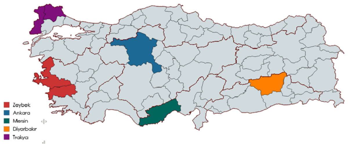
Figure 1: Geographical distribution of the five regions used in the TuFoC dataset.
The map highlights Ankara (Central Anatolia), Diyarbakır (Southeastern Anatolia), Mersin (Mediterranean region), Trakya or Thrace (European Turkey), and the Zeybek region (Western Anatolia, including İzmir and Aydın). These regions were selected for their distinct cultural, musical, and geographical characteristics to ensure diversity in the classification task.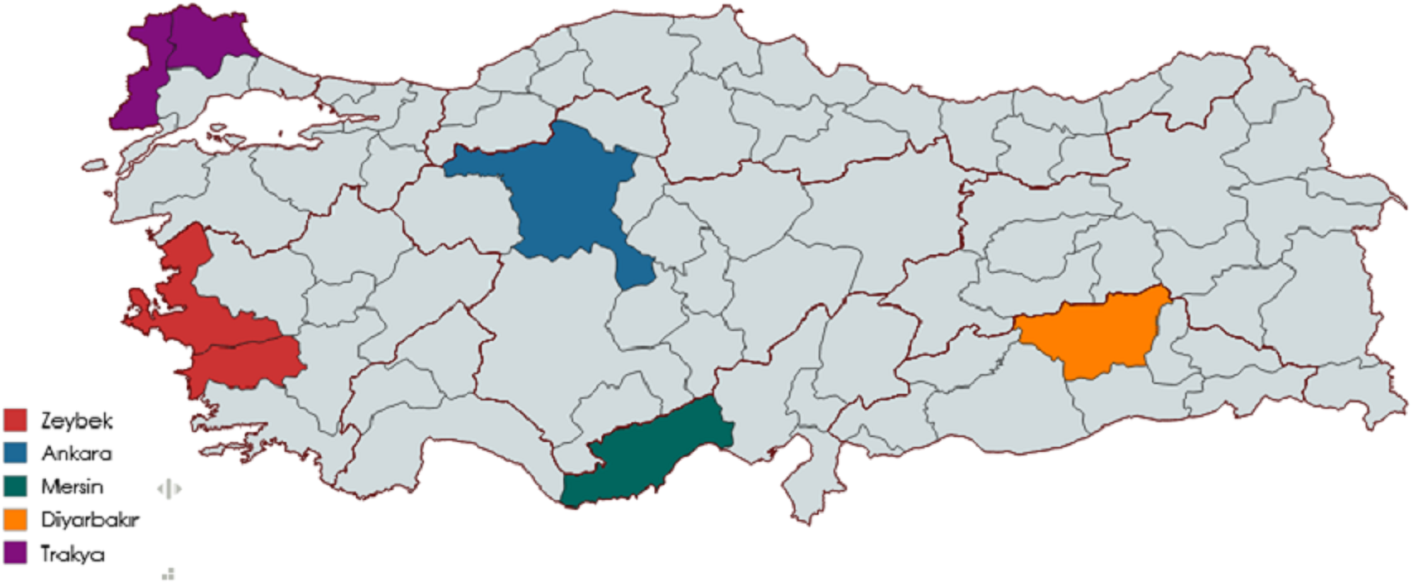
In many studies on music genre classification, neural network models are trained using features extracted from MIDI files. However, these symbolic representations often fail to capture the nuanced performance characteristics inherent to traditional music. In this study, we deliberately avoided using MIDI and extracted features directly from MP3 recordings. This approach preserves the unique performance details of each region, including ornamentation, tempo rubato, and vocal articulation, which are critical to a reliable regional classification. Mel spectrograms, representing the time-frequency energy distribution of the audio, were chosen as the primary input representation for both CNN- and LSTM-based models.
To construct region labels, we relied on a combination of accompanying metadata, archival documentation, and ethnomusicological references linked to the original field recordings. We adopted a conservative curation strategy since regional boundaries in Turkish folk music are often fluid and culturally defined rather than strictly geographic. Only those recordings with clearly documented and widely accepted regional origins were included in the dataset. Ambiguous cases—particularly those plausibly belonging to multiple neighboring regions—were deliberately excluded to reduce labeling noise and ensure dataset integrity. This approach prioritizes minimizing intra-regional overlap over enforcing rigid regional taxonomies. Nevertheless, we recognize that regional attribution remains inherently interpretive, and future studies may benefit from formal expert annotation or multi-rater consensus to validate the labels further.
Against this background, the regional classification of Turkish folk music recordings enables the identification of points of similarity, divergence, and cultural connection among works from different areas. Developed with this purpose, TuFoC aims to systematically organize Turkish folk music based on regional origin, thereby facilitating analysis of how historical and geographical factors shape musical styles. Two deep learning models—CNN and LSTM—were employed to address this classification task. The original dataset (OD) comprises 369 recordings from five delineated regions. Audio augmentation techniques such as pitch shifting and time stretching were applied to enhance model performance and mitigate overfitting, resulting in the gently augmented dataset (GAD) with 1,479 total samples. These datasets were used to train and evaluate the models under various conditions. As regional representation varied, both balanced and slightly unbalanced splits were constructed to ensure fair training and evaluation across regions.
To ensure consistency, each file was downsampled to 22.05 kHz with Librosa (McFee et al., 2015) and converted to mono. Regional labels were assigned based on metadata and ethnomusicological sources. The dataset includes well-represented and underrepresented regional categories, which were subsequently used in classification experiments.
Feature extraction
In this study, Mel spectrograms were extracted directly from MP3 recordings of Turkish folk songs to preserve the performance characteristics unique to each regional style. Unlike symbolic formats such as MIDI, MP3 recordings retain nuanced articulation, dynamics, and ornamentation, which are critical for capturing regional musical identity.
The Mel spectrograms were computed using librosa with 128 Mel bands. The Mel scale approximates human auditory perception and is defined by the formula: (1)
where f is the frequency in Hz. This transformation provides a perceptually meaningful representation of pitch and is commonly used in speech and audio classification tasks.
Each MP3 file was loaded using the librosa library with its native sampling rate preserved (i.e., sr=sr), which typically corresponds to 22.05 kHz for most MP3 recordings, thereby avoiding unnecessary resampling and maintaining the fidelity of the original audio signals. The average duration of the samples was approximately 11 s. The STFT was applied to generate Mel spectrograms, which represent the signal’s power in the Mel scale of frequency bands over time, using a window size (n_fft) of 2,048 samples and a hop length of 512 samples. A total of 128 Mel frequency bins (n_mels=128) were computed for each frame, capturing the perceptually meaningful frequency content of the audio. This visual format facilitates the use of computer vision models for audio classification.
The resulting spectrograms were standardized across samples and prepared in two formats depending on the model architecture. For the CNN model, the Mel spectrograms were normalized and saved as 2D PNG images of size 128 × 128 × 3, representing RGB-encoded spectrograms. For the LSTM model, the spectrograms were retained in their original matrix form with shape 128 × 128 (time steps × frequency bins), and fed directly as sequential input to the network.
This approach ensured no region-specific performance detail was lost during preprocessing, allowing both CNN and LSTM architectures to learn from rich acoustic representations of Turkish folk music.
Data augmentation
In addition to the original dataset, this study applied data augmentation to improve model generalization and mitigate the effects of limited and imbalanced data. Turkish folk music exhibits regional variation through nuanced performance elements such as timing, articulation, and ornamentation. However, the available dataset contains a limited number of recordings for some regions, and performances often reflect a narrow stylistic range.
To address this, controlled audio-level augmentation techniques were applied, including pitch shifting, time stretching, and the addition of low-amplitude Gaussian noise. These transformations simulate natural vocal or instrumental performance variations, mimicking real-world scenarios such as slight tempo changes, tuning differences, or environmental noise. Importantly, they preserve the class label of the original recording while enriching the diversity of the training set.
To further illustrate the effect of augmentation on spectral content, Fig. 2 presents a comparison of the Mel spectrograms from original (OD), strongly augmented (AD), and gently augmented (GAD) versions for one representative sample from each region. While AD transformations clearly shift or compress spectral bands and modulate temporal dynamics aggressively, GAD transformations exhibit milder alterations. This visual comparison supports our observation that GAD maintains the spectral integrity required for effective feature extraction and classification, unlike AD, which may introduce artifacts that hinder model generalization.
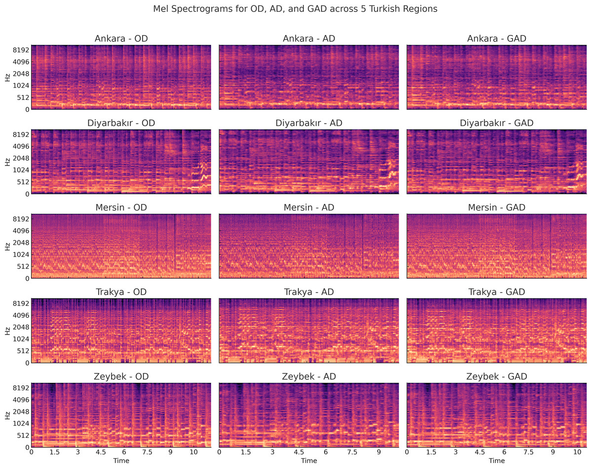
Figure 2: Comparison of Mel spectrograms across original (OD), strongly augmented (AD), and gently augmented (GAD) versions for representative recordings from five regions.
Each row shows one regional example with its three augmentation states. Visual inspection reveals that aggressive augmentations (AD) introduce more spectral distortion than GAD, which preserves core temporal and spectral features more faithfully.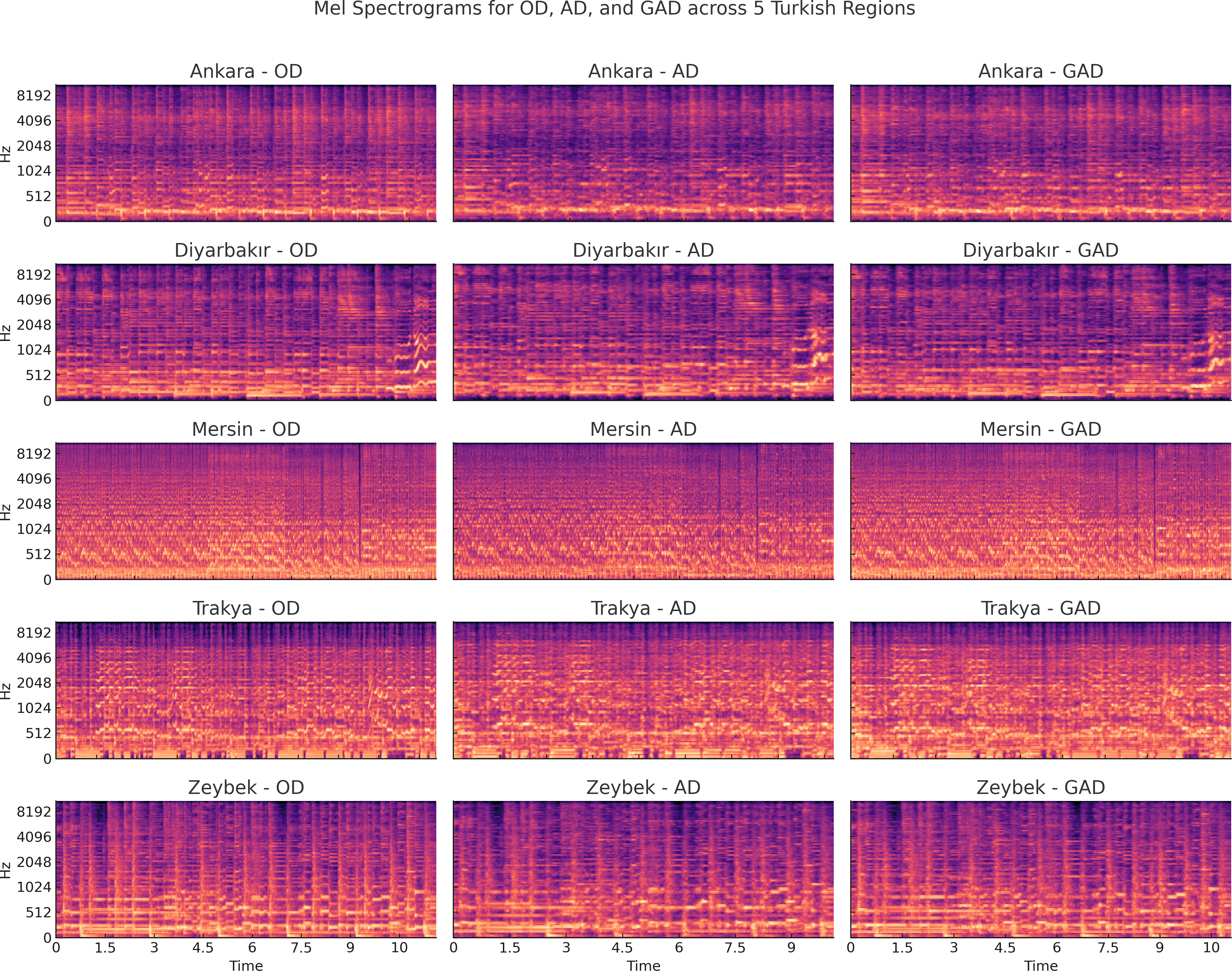
By exposing the model to varied but valid forms of regional performance, data augmentation aims to reduce overfitting, improve robustness, and enhance the model’s ability to generalize to unseen recordings, especially for underrepresented classes. This study tested two augmentation strategies: an original method involving relatively strong transformations, and a second, gentler approach designed to preserve musical features better. A comparison of these two approaches is provided in Table 1.
-
Original augmentation: Applied relatively strong transformations including pitch shifting (±2 semitones), time stretching (0.8–1.25x), and additive Gaussian noise (amplitude range: 0.001–0.015).
-
Gentle augmentation: Applied musically realistic transformations with reduced intensity: pitch shift (±1 semitone), time stretch (0.95–1.05x), and Gaussian noise (amplitude: 0.001–0.005).
Each original audio sample was augmented three times, and the resulting Mel spectrograms were included in the dataset under the same class label. The gentle augmentation strategy ultimately yielded higher classification performance and was selected as the preferred method. As these techniques are applied, the number of samples provided for the classification models is listed in the Table 2 to obtain 1,479 audio samples.
| Augmentation parameter | Original augmentation | Gentle augmentation |
|---|---|---|
| Pitch shift range | ±2 semitones | ±1 semitone |
| Time stretch range | 0.8 to 1.25 | 0.95 to 1.05 |
| Gaussian noise amplitude | 0.001 to 0.015 | 0.001 to 0.005 |
| Number of augmentations per file | 3 | 3 |
| Applied to all classes | Yes | Yes |
| Transformations per sample | Multiple combined | Multiple combined (with reduced impact) |
| Region | Original (OD) | Augmented (AD) | Gently augmented (GAD) | Total |
|---|---|---|---|---|
| Ankara | 77 | 231 | 231 | 308 |
| Diyarbakır | 72 | 219 | 219 | 291 |
| Mersin | 63 | 189 | 189 | 252 |
| Trakya | 68 | 204 | 204 | 272 |
| Zeybek | 89 | 267 | 267 | 356 |
| Total | 369 | 1,110 | 1,110 | 1,479 |
Classical baseline: LightGBM with SMOTE
To provide a fair and critical comparison with earlier work, we implemented a classical machine learning baseline inspired by Börekci & Sevli (2024). Their original study employed handcrafted audio features followed by ensemble classifiers. In our replication, we extracted histogram of oriented gradients (HOG) features from the Mel spectrogram images and trained a LightGBM classifier using SMOTE oversampling to address class imbalance. The baseline model was evaluated under the same stratified 10-fold cross-validation protocol as our deep learning models, using the OD, AD, and GAD datasets for a comprehensive performance comparison.
It is important to emphasize that SMOTE was applied only in the traditional machine learning baseline to generate synthetic feature vectors for minority classes in the HOG feature space. SMOTE creates new samples by interpolating between existing instances in the feature space, thereby improving classifier robustness without simple duplication (Zaman et al., 2024). In contrast, the CNN and LSTM models addressed class imbalance through audio-level data augmentation (i.e., AD and GAD) and were trained directly on spectrogram inputs without any synthetic oversampling techniques. While both approaches aim to improve model robustness under imbalanced data conditions, they operate on distinct data representations—handcrafted features versus raw spectrograms—and should not be conflated.
Model architecture
The architecture of TuFoC includes two deep learning models trained on Mel spectrograms: (1) a CNN model utilizing transfer learning with a pre-trained MobileNetV2, and (2) a RNN model based on LSTM units. The CNN architecture (LeCun et al., 1998) was chosen for its spatial pattern recognition capabilities, while the LSTM model (Hochreiter & Schmidhuber, 1997) was designed to capture temporal dependencies in sequential data. Both models were trained on Mel spectrogram representations of audio recordings, with additional experiments conducted using data augmentation strategies to enhance model generalization. Although both approaches were tested, the CNN architecture consistently outperformed the LSTM model in terms of accuracy, stability, and generalizability.
MobileNetV2-Based CNN Model
The first model is based on the MobileNetV2 architecture, a lightweight convolutional neural network originally designed for image classification tasks and pretrained on the ImageNet dataset. Despite the domain mismatch between natural images and audio spectrograms, prior research has shown that transfer learning from large-scale visual datasets can still be effective in audio-related tasks. This is because spectrograms, while representing audio data, exhibit visual characteristics such as local textures, frequency edges, and time-dependent patterns analogous to those in natural images. Therefore, convolutional filters pretrained on ImageNet can still provide valuable feature extraction capabilities for spectrogram inputs, particularly in the lower layers of the network.
Each MP3 audio file was converted into a 128 × 128 Mel spectrogram, normalized, and saved as a three-channel RGB image. These images served as input to the CNN model. The base layers of MobileNetV2 were frozen to retain general-purpose features, while a custom classification head was appended. This included a global average pooling layer, a dense layer with 128 ReLU-activated units, a dropout layer with a rate of 0.3, and a final softmax layer for classification. The model was trained using the Adam optimizer and categorical cross-entropy loss. To improve generalization, standard image augmentation techniques—such as horizontal flipping, rotation, zooming, and shifting—were applied during training. A summary of the CNN model’s hyperparameters is presented in Table 3.
| Hyperparameter | CNN (MobileNetV2) | LSTM model |
|---|---|---|
| Input shape | 128 × 128 × 3 | 128 × 128 (time × Mel bins) |
| Pretrained weights | ImageNet | None |
| Frozen base layers | Yes | N/A |
| Trainable parameters | Final classifier head | All |
| Optimizer | Adam | Adam |
| Loss function | Categorical cross-entropy | Categorical cross-entropy |
| Dropout rate | 0.3 | 0.3 (standard) + 0.2 (recurrent) |
| Hidden units (dense/LSTM) | Dense: 128 (ReLU) | LSTM: 128 + Dense: 64 (ReLU) |
| Batch size | 32 | 32 |
| Epochs | 100 | 100 |
| Early stopping | Patience = 15 | Patience = 15 |
| Data augmentation | Yes (image) | No |
| Masking for variable input | N/A | Yes |
| Evaluation method | 10-fold cross-validation | 10-fold cross-validation |
The input shape and processing differ between the CNN and LSTM models. While the CNN receives 3-channel images of shape 128 × 128 × 3, the LSTM operates directly on the raw spectrogram matrices as 2D sequences of shape 128 × 128, treating each row as a time step and each column as a frequency bin. The model is also given in Fig. 3.
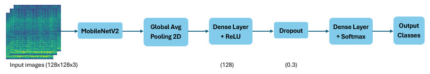
Figure 3: Architecture of the CNN model used for regional classification of Turkish folk music samples, based on MobileNetV2 with transfer learning.
The input is a 128×128 Mel spectrogram image representing the full duration of a musical excerpt. The model begins with a MobileNetV2 backbone pretrained on ImageNet, which is adapted through fine-tuning for the task. The convolutional base extracts low- to high-level spectral features from the input. A global average pooling layer reduces spatial dimensions while preserving feature richness, followed by fully connected layers that map to five output neurons, each representing a musical region. This architecture emphasizes computational efficiency and strong generalization on moderately sized cultural datasets.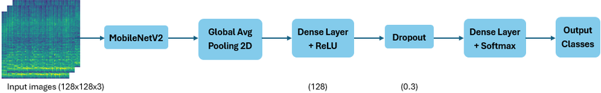
Although MobileNetV2 was initially developed for natural images, its strong performance on spectrogram classification tasks has been documented in studies involving music genre classification, environmental sound tagging, and speech recognition, reinforcing its suitability for this study’s spectrogram-based input.
LSTM-based sequence model
The second model treats Mel spectrograms as 2D time-frequency matrices, interpreting them as sequences along the temporal axis. Each spectrogram was extracted as a NumPy array of shape (128, 128), where the 128 rows represent time frames and the 128 columns correspond to Mel frequency bins. For use in a sequential model, the data were reshaped to treat each time frame as a single time step with 128 input features.
The architecture comprises a single unidirectional LSTM layer with 128 hidden units, designed to capture temporal dependencies within the spectrogram sequence. To improve regularization, dropout with a rate of 0.3 was applied after the LSTM layer, while recurrent dropout with a rate of 0.2 was employed within the LSTM cell during training. Following the LSTM, a dense layer with 64 ReLU-activated units processes the temporal representation before passing it to a final softmax layer that performs classification across the five regional classes. To support variable-length inputs, masking ignored zero-padded segments during training. Given the relatively small dataset, the number of hidden units was chosen empirically through preliminary tuning to balance learning capacity with the risk of overfitting. A complete summary of the LSTM model’s hyperparameters is provided in Table 3. The model architecture is also illustrated in Fig. 4.
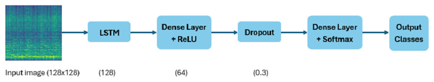
Figure 4: Architecture of the LSTM model designed for regional classification of Turkish folk music samples.
The input is a time-sequence representation reshaped from a 128×128 Mel spectrogram image, where each row is treated as a temporal frame. The model consists of a single unidirectional LSTM layer that processes the sequential data to capture temporal dependencies within the audio. This is followed by a fully connected (dense) output layer with five units, each representing one of the target regional music classes. This architecture serves as a baseline for evaluating the effectiveness of recurrent neural networks on spectrogram-based audio features.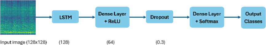
This architecture is designed to capture the temporal evolution of spectral features that may characterize regional stylistic elements, such as rhythmic patterns or evolving timbral textures. The model was trained using the Adam optimizer and categorical cross-entropy loss, with early stopping applied based on validation loss.
While a single-layer LSTM was used in this study for simplicity and to reduce overfitting risk on a small dataset, alternative architectures such as gated recurrent units (GRUs), bidirectional LSTMs, or attention-based models may provide improved temporal modeling and are worth exploring in future work.
Evaluation strategy
To evaluate the performance of the models in the TuFoC framework, stratified 10-fold cross-validation was applied and repeated over 30 independent runs. This approach preserved the class distribution within each fold and enabled consistent training and testing across multiple partitions. All Mel spectrogram data were loaded into memory and split using the StratifiedKFold method from the scikit-learn library. The model’s performance was assessed for each fold using four key metrics: accuracy, precision, recall, and macro F1-score. These metrics were computed per fold, and final results were reported as the mean ± standard deviation across all folds. To mitigate variability due to random weight initialization and data shuffling, each experiment was repeated independently 30 times, and all reported metrics were averaged across these runs.
The evaluation results for the CNN and LSTM models across all datasets are presented in Table 4. Statistical significance between model performances was assessed using paired t-tests across the 30-run distributions. The details of the training setup, dataset splits, and implementation parameters are provided in Section ‘Experimental Setup’.
Experimental Setup
All experiments were conducted on a system equipped with an NVIDIA GPU and 16 GB of RAM, running Python 3.7 with TensorFlow and Keras libraries. The training procedures, preprocessing pipeline, and data augmentation strategies were standardized across all models and experimental conditions to ensure a fair comparison.
Each model was trained for a maximum of 100 epochs using the Adam optimizer and categorical cross-entropy loss function, with a batch size of 32. To prevent overfitting and select the best-performing model, early stopping was applied based on validation loss, with a patience value of 15 epochs. When triggered, the model automatically restored the weights from the epoch that achieved the lowest validation loss. This strategy helped enhance generalization and reduce unnecessary training.
The same input shapes, normalization steps, and class label encodings were applied across both CNN and LSTM pipelines. Model-specific hyperparameters, such as using pretrained MobileNetV2 layers in the CNN and recurrent dropout in the LSTM, are detailed in Table 3.
To prevent overfitting and improve generalization, early stopping was employed during training. Validation loss was monitored as the stopping criterion, with a patience value of 15 epochs. If no improvement was observed for 15 consecutive epochs, training was halted, and the model weights were automatically restored to those from the epoch with the lowest validation loss. This approach ensured that training was efficient and adaptive, avoiding unnecessary over-training while preserving the best-performing model on validation data.
| Model | Dataset | Accuracy (%) | Precision (%) | Recall (%) | Macro F1-score (%) |
|---|---|---|---|---|---|
| CNN | OD | 90.00 ± 4.00 | 90.00 ± 4.00 | 90.00 ± 4.00 | 89.00 ± 4.00 |
| CNN | AD | 88.00 ± 1.00 | 88.00 ± 1.00 | 88.00 ± 2.00 | 88.00 ± 2.00 |
| CNN | GAD | 92.68 ± 1.60 | 92.63 ± 1.53 | 92.41 ± 1.62 | 92.38 ± 1.64 |
| LSTM | OD | 51.00 ± 8.00 | 54.00 ± 12.00 | 50.00 ± 8.00 | 49.00 ± 10.00 |
| LSTM | AD | 59.00 ± 5.00 | 60.00 ± 5.00 | 59.00 ± 5.00 | 59.00 ± 5.00 |
| LSTM | GAD | 74.67 ± 4.75 | 75.02 ± 4.35 | 74.19 ± 4.66 | 73.89 ± 4.87 |
Evaluation metrics
Four widely used evaluation metrics—accuracy, precision, recall, and F1-score—were adopted to evaluate the CNN and LSTM models’ classification performance. These metrics provide a comprehensive view of the models’ effectiveness in multi-class classification tasks, especially in scenarios with limited or imbalanced data.
Results
The classification performance of both the CNN and LSTM models was evaluated across 30 independent runs using 10-fold cross-validation. Each model was tested on both the original dataset (OD), the augmented dataset (AD) and the dataset augmented using gentle audio-level transformations (GAD). The performance metrics, including accuracy, precision, recall, and macro F1-score, are summarized in Table 4.
The CNN model consistently demonstrated superior performance across all dataset configurations. On the OD, it achieved an average accuracy of 90.00% and a macro F1-score of 89.00%. Performance improved further with augmentation: on the GAD, the CNN reached 92.68% accuracy and 92.38% macro F1-score.
The LSTM model, while conceptually aligned with the sequential nature of audio data, delivered substantially lower performance. On the OD, it achieved 51.00% accuracy and 49.00% macro F1-score, with significant variability across folds. With gentle augmentation (GAD), its performance improved to 74.67% accuracy and 73.89% macro F1-score, indicating that data augmentation positively affected its ability to generalize. Nevertheless, it remained less effective than the CNN, particularly in handling complex spectral variations. Even in its best-case setting (GAD), the LSTM fell short of CNN’s performance on the original dataset, confirming CNN’s superior capacity for spectro-temporal pattern extraction.
This performance gap can be attributed to the CNN’s ability to extract spatial features from Mel spectrograms, which visually encode time–frequency structures effectively. In contrast, the LSTM model was more sensitive to data scarcity and less suited to capturing local spectral details in relatively small and imbalanced datasets. Furthermore, while image-based augmentations benefited the CNN, the LSTM pipeline did not employ sequence-level augmentation, possibly limiting its generalization capacity.
To further validate these findings, we calculated 95% confidence intervals and Cohen’s d effect sizes based on the 30-run results. The CNN achieved an accuracy of 92.68% (95% CI [92.08%–93.28%]) and a macro F1-score of 92.38% ([91.77%, 92.99%]), while the LSTM yielded 74.67% accuracy ([72.90%, 76.45%]) and 73.89% macro F1-score ([72.07%, 75.71%]). Cohen’s d exceeded 5.0 in both comparisons, confirming a very large effect size.
To assess whether the observed differences in model performance across the OD, AD, and GAD datasets were statistically significant, we performed one-way analysis of variance (ANOVA) tests followed by Tukey’s HSD post hoc comparisons. Table 5 summarizes the ANOVA results for both CNN and LSTM models, using accuracy and macro F1-score as evaluation metrics over 30 independent runs. All tests returned highly significant p-values (<10−9), confirming that dataset configuration significantly affects model performance. Notably, the LSTM model exhibited a larger F-value, indicating a stronger effect of dataset variation. This aligns with our earlier findings that LSTM performance is particularly sensitive to the quality of augmentation. The subsequent Tukey HSD tests revealed that GAD significantly outperformed both OD and AD in most settings. These results statistically validate the performance improvements attributed to gentle augmentation.
| Model | Metric | F-value | p-value | Significance |
|---|---|---|---|---|
| CNN | Accuracy | 27.23 | 6.56 × 10⁻¹⁰ | Significant |
| CNN | Macro F1-score | 26.78 | 8.63 × 10⁻¹⁰ | Significant |
| LSTM | Accuracy | 116.11 | 2.76 × 10⁻²⁵ | Highly significant |
| LSTM | Macro F1-score | 90.13 | 6.27 × 10⁻²² | Highly significant |
An inspection of the confusion matrices revealed consistent trends in regional classification performance. The CNN model showed strong diagonal dominance across all regions, with particularly high precision for geographically distant or stylistically distinct regions. Misclassifications tended to occur between neighboring or culturally overlapping regions, such as those sharing similar melodic phrasing or instrumentation. The LSTM model, in contrast, exhibited greater dispersion across off-diagonal elements, often confusing these adjacent regions more frequently, suggesting limited capacity to resolve subtle acoustic cues in the spectrogram sequences.
The CNN model achieved an average accuracy of 92.7% on the GAD. This performance is comparable to accuracies reported in genre classification tasks using CNNs and Mel spectrograms on benchmark datasets such as GTZAN and FMA, where transfer learning-based models (e.g., MobileNetV2) typically achieve between 85% and 92% accuracy (Choi, Fazekas & Sandler, 2017; Pons & Serra, 2019; Zhang et al., 2016). This contextualizes TuFoC’s effectiveness despite the challenges of cultural specificity and limited data.
In terms of performance variability, the CNN model demonstrated high consistency across 30 runs, with narrow confidence intervals and relatively stable fold-to-fold performance. This stability is likely attributable to its use of spatial feature extraction and pretrained weights, which enhanced its generalization even under modest data conditions. The LSTM model, however, showed higher variance, both across runs and within folds, particularly on the Original Dataset. This suggests that without sequence-level augmentation or architectural enhancements, the LSTM struggled to converge reliably on consistent patterns from the input data.
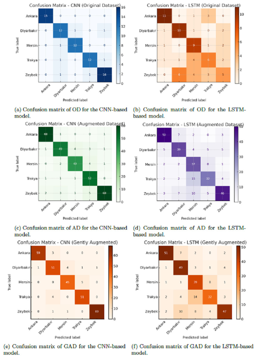
Figure 5: Confusion matrices of CNN and LSTM models across three datasets: original dataset (OD), augmented dataset (AD), and gently augmented dataset (GAD).
In each matrix, rows represent true region labels and columns represent predicted labels. Darker diagonal cells indicate more correct predictions, while off-diagonal cells signify misclassifications. CNN matrices exhibit clear diagonal dominance, particularly on GAD, demonstrating strong classification performance. LSTM matrices reveal more frequent confusion between classes, especially for regions that are geographically and stylistically similar. This visual comparison illustrates the differential impact of augmentation and architecture on classification accuracy.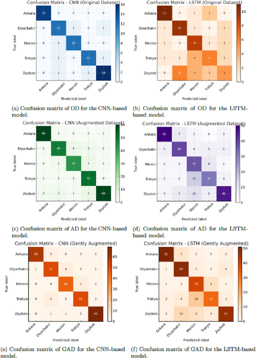
Confusion matrices visualizing the class-specific predictions across datasets and models are shown in Fig. 5. These highlight consistent misclassifications in the LSTM model, particularly for regions with more subtle stylistic distinctions. To engage directly with the approach of Börekci & Sevli (2024), we replicated a similar traditional machine learning pipeline by training a LightGBM classifier on HOG features extracted from Mel spectrograms, combined with SMOTE oversampling to handle class imbalance. As presented in Table 6, this baseline achieved competitive results, particularly on the GAD, reaching an accuracy of 92.53% and a macro F1-score of 92.53%. However, our proposed CNN model not only marginally outperformed the LGBM baseline on GAD (92.68% accuracy vs. 92.53%), but also demonstrated consistently superior results across all dataset configurations when compared to the LSTM model. While data augmentation significantly improved LSTM performance—particularly on GAD—it remained substantially less effective than CNN, highlighting the latter’s stronger generalization and robustness.
To promote transparency and enable reproducibility, Tables 7, 8 and 9 provide the complete performance values for all 30 runs across different datasets and models, which form the basis of the statistical analyses reported in this section.
More importantly, the CNN architecture offers substantial advantages in modeling high-level spatial and temporal relationships embedded in Mel spectrograms—something handcrafted feature pipelines inherently struggle to capture. Furthermore, unlike the static modeling approach of Börekci & Sevli (2024), our method integrates a learnable feature hierarchy, enabling end-to-end training without manual feature design. This marks a clear contribution in terms of methodological novelty. Additionally, the comparative underperformance of the LSTM model on OD and AD, and its significant improvement on GAD, further underscores the importance of our preprocessing and augmentation strategy in enhancing model generalizability. Overall, the results not only validate the effectiveness of deep learning over traditional pipelines, but also demonstrate that our model contributes a more flexible, scalable, and data-driven approach to regional classification in Turkish folk music.
Discussion
The comparative analysis of CNN and LSTM architectures reveals key insights into the suitability of deep learning models for regional music classification based on spectrogram data. CNNs, due to their convolutional structure, are inherently well-suited for analyzing 2D representations such as Mel spectrograms. Their ability to capture local spatial patterns across frequency and time axes provides a significant advantage in recognizing region-specific spectral textures.
| Model | Dataset | Accuracy (%) | Precision (%) | Recall (%) | F1-score (%) |
|---|---|---|---|---|---|
| LightGBM + SMOTE | OD | 83.15 ± 4.00 | 84.83 ± 4.17 | 83.08 ± 4.03 | 83.08 ± 4.08 |
| LightGBM + SMOTE | AD | 81.97 ± 1.87 | 82.20 ± 1.90 | 81.96 ± 1.87 | 81.92 ± 1.88 |
| LightGBM + SMOTE | GAD | 92.53 ± 2.04 | 92.73 ± 2.03 | 92.54 ± 2.03 | 92.53 ± 2.03 |
Notes:
Best results are shown in bold.
| Run | Acc_CNN | Acc_LSTM | Macro F1_CNN | Macro F1_LSTM |
|---|---|---|---|---|
| 1 | 0.8649 | 0.6081 | 0.8618 | 0.5988 |
| 2 | 0.8108 | 0.5000 | 0.8038 | 0.4920 |
| 3 | 0.8649 | 0.4595 | 0.8604 | 0.4782 |
| 4 | 0.9324 | 0.6486 | 0.9306 | 0.6213 |
| 5 | 0.9324 | 0.5541 | 0.9300 | 0.5601 |
| 6 | 0.8784 | 0.5676 | 0.8775 | 0.5613 |
| 7 | 0.8784 | 0.4054 | 0.8737 | 0.3189 |
| 8 | 0.9189 | 0.6351 | 0.9132 | 0.6214 |
| 9 | 0.9054 | 0.6081 | 0.9016 | 0.6141 |
| 10 | 0.8378 | 0.4730 | 0.8369 | 0.4074 |
| 11 | 0.9189 | 0.5135 | 0.9152 | 0.5345 |
| 12 | 0.9459 | 0.4054 | 0.9454 | 0.4194 |
| 13 | 0.9054 | 0.5676 | 0.9066 | 0.5725 |
| 14 | 0.8243 | 0.5270 | 0.8247 | 0.5340 |
| 15 | 0.9459 | 0.4595 | 0.9413 | 0.3947 |
| 16 | 0.9054 | 0.5946 | 0.9017 | 0.6027 |
| 17 | 0.9189 | 0.5811 | 0.9182 | 0.5751 |
| 18 | 0.9189 | 0.4324 | 0.9185 | 0.4394 |
| 19 | 0.8514 | 0.3919 | 0.8506 | 0.4002 |
| 20 | 0.9324 | 0.3378 | 0.9292 | 0.2163 |
| 21 | 0.8243 | 0.4459 | 0.8242 | 0.4386 |
| 22 | 0.9189 | 0.5405 | 0.9139 | 0.5312 |
| 23 | 0.9189 | 0.5135 | 0.9108 | 0.5101 |
| 24 | 0.9324 | 0.3514 | 0.9312 | 0.2731 |
| 25 | 0.9324 | 0.5000 | 0.9339 | 0.4862 |
| 26 | 0.9459 | 0.5405 | 0.9444 | 0.5129 |
| 27 | 0.8784 | 0.5405 | 0.8734 | 0.5543 |
| 28 | 0.9054 | 0.5270 | 0.8983 | 0.5255 |
| 29 | 0.8919 | 0.4865 | 0.8856 | 0.4953 |
| 30 | 0.8784 | 0.5135 | 0.8648 | 0.5145 |
| Run | Acc_CNN | Acc_LSTM | Macro F1_CNN | Macro F1_LSTM |
|---|---|---|---|---|
| 1 | 0.9189 | 0.6622 | 0.9164 | 0.6611 |
| 2 | 0.8581 | 0.5642 | 0.8531 | 0.5371 |
| 3 | 0.8919 | 0.5980 | 0.8874 | 0.5989 |
| 4 | 0.8818 | 0.5676 | 0.8777 | 0.5620 |
| 5 | 0.8581 | 0.5270 | 0.8545 | 0.5175 |
| 6 | 0.8750 | 0.6892 | 0.8712 | 0.6833 |
| 7 | 0.8784 | 0.6149 | 0.8793 | 0.6082 |
| 8 | 0.8851 | 0.6149 | 0.8820 | 0.6083 |
| 9 | 0.8716 | 0.5608 | 0.8691 | 0.5586 |
| 10 | 0.8615 | 0.5608 | 0.8574 | 0.5556 |
| 11 | 0.8547 | 0.6385 | 0.8535 | 0.6268 |
| 12 | 0.8784 | 0.5709 | 0.8771 | 0.5633 |
| 13 | 0.8885 | 0.5541 | 0.8851 | 0.5530 |
| 14 | 0.8682 | 0.6284 | 0.8631 | 0.6193 |
| 15 | 0.8818 | 0.6824 | 0.8743 | 0.6712 |
| 16 | 0.8953 | 0.4797 | 0.8926 | 0.4655 |
| 17 | 0.8986 | 0.6689 | 0.8962 | 0.6566 |
| 18 | 0.8953 | 0.5270 | 0.8939 | 0.5252 |
| 19 | 0.8818 | 0.5608 | 0.8799 | 0.5547 |
| 20 | 0.8919 | 0.6959 | 0.8884 | 0.6935 |
| 21 | 0.8750 | 0.5878 | 0.8706 | 0.5803 |
| 22 | 0.8885 | 0.6385 | 0.8870 | 0.6265 |
| 23 | 0.8818 | 0.5676 | 0.8758 | 0.5637 |
| 24 | 0.8649 | 0.5912 | 0.8649 | 0.5794 |
| 25 | 0.8581 | 0.5811 | 0.8551 | 0.5717 |
| 26 | 0.8649 | 0.5507 | 0.8612 | 0.5477 |
| 27 | 0.8851 | 0.5980 | 0.8820 | 0.5985 |
| 28 | 0.8615 | 0.5811 | 0.8548 | 0.5642 |
| 29 | 0.8784 | 0.5676 | 0.8750 | 0.5601 |
| 30 | 0.8750 | 0.5439 | 0.8734 | 0.5386 |
| Run | Acc_CNN | Acc_LSTM | Macro F1_CNN | Macro F1_LSTM |
|---|---|---|---|---|
| 1 | 0.9189 | 0.8108 | 0.9141 | 0.8054 |
| 2 | 0.9358 | 0.8108 | 0.9333 | 0.8059 |
| 3 | 0.9088 | 0.7568 | 0.9066 | 0.7498 |
| 4 | 0.9291 | 0.7703 | 0.9259 | 0.7571 |
| 5 | 0.9426 | 0.6993 | 0.9423 | 0.6968 |
| 6 | 0.9628 | 0.6993 | 0.9605 | 0.6918 |
| 7 | 0.9324 | 0.7534 | 0.9263 | 0.7462 |
| 8 | 0.9358 | 0.7027 | 0.9332 | 0.6941 |
| 9 | 0.8818 | 0.7297 | 0.8789 | 0.7214 |
| 10 | 0.9324 | 0.7196 | 0.9293 | 0.7061 |
| 11 | 0.9459 | 0.6993 | 0.9428 | 0.6910 |
| 12 | 0.9122 | 0.7534 | 0.9095 | 0.7458 |
| 13 | 0.9358 | 0.6791 | 0.9321 | 0.6801 |
| 14 | 0.9189 | 0.6824 | 0.9166 | 0.6522 |
| 15 | 0.9189 | 0.7534 | 0.9149 | 0.7471 |
| 16 | 0.9392 | 0.7432 | 0.9358 | 0.7346 |
| 17 | 0.9189 | 0.7736 | 0.9151 | 0.7744 |
| 18 | 0.9257 | 0.7432 | 0.9243 | 0.7402 |
| 19 | 0.9155 | 0.7770 | 0.9128 | 0.7708 |
| 20 | 0.9088 | 0.6926 | 0.9053 | 0.6946 |
| 21 | 0.9358 | 0.8108 | 0.9311 | 0.8067 |
| 22 | 0.9358 | 0.7466 | 0.9326 | 0.7362 |
| 23 | 0.9459 | 0.7635 | 0.9447 | 0.7562 |
| 24 | 0.9122 | 0.8209 | 0.9069 | 0.8093 |
| 25 | 0.9020 | 0.8412 | 0.8983 | 0.8314 |
| 26 | 0.9257 | 0.7264 | 0.9219 | 0.7113 |
| 27 | 0.9257 | 0.7230 | 0.9215 | 0.7155 |
| 28 | 0.9324 | 0.7635 | 0.9328 | 0.7550 |
| 29 | 0.9223 | 0.8074 | 0.9200 | 0.8027 |
| 30 | 0.9459 | 0.6486 | 0.9434 | 0.6372 |
To highlight the performance differences among the three dataset configurations—OD, AD, GAD—we refer to the classification results summarized in Table 4. These results, based on 30 runs of stratified 10-fold cross-validation, demonstrate that GAD consistently yields superior accuracy, precision, and F1-scores across both CNN and LSTM models. This improvement underscores the importance of domain-sensitive augmentation strategies that enhance model generalization while preserving the authenticity of musical content. The observed performance gap between aggressive and gentle augmentation approaches stems from the nature of the transformations applied. Techniques such as wide-range pitch shifting and substantial time stretching, while common in speech or environmental sound processing, can distort the musically salient features in traditional music.
In Turkish folk music, regional distinctions often depend on culturally embedded pitch contours, timbral textures, and microtonal nuances. Excessive modification of these elements may introduce artificial patterns that misrepresent regional identity, thereby weakening the association between input features and class labels. In contrast, the gentle augmentation strategy applied in this study was carefully crafted to preserve these stylistic traits by limiting the intensity of transformations. As evidenced in Table 4, models trained on GAD consistently outperform those trained on AD, confirming that musically coherent variability supports better generalization in region-based classification.
The use of MobileNetV2 in this study was motivated by its efficiency, strong generalization in low-data regimes, and its proven transferability across domains. Rather than proposing a novel architecture, the contribution lies in adapting a lightweight pretrained CNN to the underexplored task of regional music classification based on culturally specific, non-Western audio content. Given the scarcity of large-scale, labeled folk music datasets, transfer learning from ImageNet was a practical and effective strategy to mitigate overfitting while leveraging robust feature extraction.
The confusion matrix of the CNN model on the GAD (Fig. 5) further illustrates the model’s classification behavior. High values along the diagonal indicate strong per-region accuracy, while the few misclassifications observed typically occur between geographically or stylistically adjacent regions. This suggests that the model captures musically plausible patterns of regional overlap rather than making random errors. Although a detailed interpretability analysis is beyond the scope of this study, the confusion patterns provide preliminary evidence that the CNN has learned features aligned with cultural and musical proximity.
All evaluation procedures, including cross-validation and final performance reporting, were conducted on the respective held-out test folds of each dataset variant (OD, AD, or GAD), ensuring that predictions were always made on unaltered samples within the context of each augmentation strategy.
Rather than introducing architectural novelty, this study focuses on adapting a lightweight pretrained CNN to a culturally specific and data-constrained classification task. The contribution lies in demonstrating the effectiveness of transfer learning using Mel spectrograms in the context of regional style detection within Turkish folk music.
On the other hand, the LSTM model, while theoretically appropriate for modeling temporal dependencies, showed limited effectiveness in this setting. The sequential input format used for spectrogram slices may have diluted spatial coherence, and the model’s sensitivity to small datasets likely contributed to underperformance. Furthermore, the absence of sequence-aware data augmentation may have hindered the model’s robustness. The LSTM configuration used in this study was intentionally kept simple to serve as a baseline for evaluating temporal modeling on spectrogram-derived input. More advanced designs, such as bidirectional LSTMs, attention-equipped RNNs, or CRNNs, may yield stronger performance, but were excluded here to isolate the comparative behavior of basic recurrent and convolutional models under identical conditions.
The success of the CNN model in this study reinforces the practicality of using 2D convolutional networks for audio classification tasks where temporal structure is implicitly embedded in the input representation. While LSTMs remain valuable in contexts where raw waveform or symbolic sequences are available, their utility for spectrogram-based regional style classification appears limited without architectural or data-level enhancements.
These findings suggest that future architectures for regional music classification should either prioritize convolutional feature extraction or explore hybrid models (e.g., CRNNs) that combine spatial and temporal representations more effectively.
While augmentation techniques were applied to improve model training, it is important to clarify that all evaluations—including stratified 10-fold cross-validation and final testing—were conducted using the original, unaltered recordings. Augmentation was used only during training to improve generalization and reduce overfitting. Therefore, the proposed system is suitable for real-world applications, where classification operates on genuine, non-augmented folk song recordings.
Limitations
Despite its promising results, this study has several limitations. First, the dataset is relatively small, and while augmentation techniques help, they cannot fully replace authentic data diversity. Second, the classification was limited to five regions. Incorporating more fine-grained regional or stylistic subcategories could provide deeper insights. Third, while we replicated a traditional machine learning baseline, the work does not explore other modern deep learning architectures such as attention mechanisms or transformer-based models, which could further enhance classification robustness.
Conclusions
This study proposed a deep learning-based regional classification framework for Turkish folk music recordings using Mel spectrograms. By introducing the TuFoC dataset—consisting of 369 recordings labeled across five cultural regions—and combining it with modern neural architectures, we demonstrated that regional music classification is feasible even in low-resource settings. Our findings also suggest that spectrogram-based models can learn to capture culturally salient audio features without requiring explicit feature engineering.
Beyond its technical contributions, the study also advances the computational analysis of traditional music cultures by offering an interpretable classification of Turkish folk music across geographic regions. The proposed models enable nuanced insights into regional stylistic variation and can serve as a foundation for future studies focused on harder-to-classify overlaps in geographically adjacent musical traditions.
We implemented two distinct architectures: a CNN model leveraging transfer learning via MobileNetV2, and an LSTM model to capture temporal evolution in spectral data. We evaluated performance under three training settings: OD, AD, GAD. Among these, GAD consistently yielded the highest classification performance. The CNN model trained on GAD achieved 92.68% accuracy, 92.63.1% precision, and 92.38% macro-averaged F1-score. These results highlight the importance of perceptually informed augmentation and demonstrate the advantages of deep learning models when learning from raw audio inputs.
Future work will focus on expanding the dataset with more regionally balanced examples and incorporating metadata such as instrument types, performer identities, or lyric content. Additionally, we plan to investigate self-supervised pretraining and transformer-based architectures to improve generalization, particularly for underrepresented categories. Another possible direction involves adapting the model for multi-label classification to reflect hybrid regional characteristics that are often found in Turkish folk music traditions.