
Enhanced congestion prediction of traffic flow using a hybrid attention-based deep learning model
- Published
- Accepted
- Received
- Academic Editor
- José Alberto Benítez-Andrades
- Subject Areas
- Algorithms and Analysis of Algorithms, Artificial Intelligence, Data Mining and Machine Learning, Optimization Theory and Computation, Neural Networks
- Keywords
- Convolutional neural network, Bi-directional long short-term memory, Congestion prediction
- Copyright
- © 2025 Aburasain
- Licence
- This is an open access article distributed under the terms of the Creative Commons Attribution License, which permits unrestricted use, distribution, reproduction and adaptation in any medium and for any purpose provided that it is properly attributed. For attribution, the original author(s), title, publication source (PeerJ Computer Science) and either DOI or URL of the article must be cited.
- Cite this article
- 2025. Enhanced congestion prediction of traffic flow using a hybrid attention-based deep learning model. PeerJ Computer Science 11:e3224 https://doi.org/10.7717/peerj-cs.3224
Abstract
Traffic congestion has become a critical issue worldwide, significantly impacting the quality of life and causing economic losses in urban areas. To address this, the concept of smart cities has emerged, utilizing technologies like artificial intelligence (AI), machine learning (ML), and the Internet of Things (IoT) to optimize transportation systems. One of the main challenges in smart city traffic management is accurately predicting traffic congestion. Existing approaches often struggle with providing reliable predictions, especially in cloud-based environments, which can lead to inaccurate traffic estimates. This article, propose a novel data-driven approach to predict traffic congestion in smart cities using a hybrid model that combines bi-directional long short-term memory (Bi-LSTM), convolutional neural networks (CNN), and an attention network. This model leverages factors such as traffic conditions, road types, and weather data to improve prediction accuracy. The model’s performance is evaluated using key metrics including root mean squared error (RMSE), mean squared error (MSE), and mean absolute error (MAE), across four junctions (J1, J2, J3, J4). The proposed model consistently outperforms existing methods, including gated recurrent unit (GRU), long short-term memory (LSTM), CNN, and multi-layer perceptron (MLP). In Junction 1, the proposed model achieved the best results with RMSE = 0.252, MSE = 0.063, and MAE = 0.178. In Junction 2, the proposed model again led with RMSE = 0.561, while other models, like GRU and LSTM, showed higher error rates. These results confirm that the hybrid model is more effective at predicting traffic congestion, particularly in dynamic urban environments. The proposed approach offers a promising solution for improving traffic flow and optimizing smart city infrastructure.
Introduction
The everyday lives of individuals and traffic management greatly depend on accurate and timely short-term traffic (STT) flow prediction. It has the ability to assist government organizations in creating enhanced path ideas to lessen accidents as well as traffic congestion, in addition to serving visitors make improved path recommendations to protect money along with time (Zheng, Liu & Hsu, 2020). In recent years, traffic flow prediction (TFP) techniques have received a lot of interest as a possible remedy for traffic jams and as a means of constructing a safer traffic network. However, they often exhibit poor efficiency and require larger computational expenses when utilized in more complex road networks. This uses a simple tree structure as the fundamental unit to mimic the supplied road network (Sun, Li & Zhang, 2020).
Traffic congestion is a major problem in town regions since it affects the economy, the environment, and air quality. To increase the effectiveness and capacity of traffic management, sustainable transportation systems (STSs) are essential for traffic congestion prediction and the adoption of transportation networks (Anjaneyulu & Kubendiran, 2022). The goal in this article is to enhance the prediction model’s characteristics, which will be useful when using the model in practical settings. The deep aggregation structure which is a sequence-to-sequence structure of the gated recurrent unit (GRU) as well as graph convolutional network (GCN) are the tools use to demonstrate a novel hybrid deep learning (DL) model (Boukerche & Wang, 2020).
An existing article develops and implements a hybrid model for urban expressway lane-level mixed TFP, grounded on DL. The model consists of three modules. This model investigates the phenomenon of traffic flow’s reciprocal impact on different lanes and the interplay between traffic flows and different types of traffic. Precise real-time TFP is critical for route direction as well as traffic fine control (Gao et al., 2024). To address the problem of insufficient data, this research augments ML algorithms for STT prediction using transfer learning methodologies. Highways England sourced every of the traffic data employed from the UK road networks. When training a model, it is unusual for every connection in a city to have access to the massive amounts of historical data required (Li et al., 2021).
The use of DL methods for criticism resolution is growing in importance. Recent studies have collected data on DL applications in transportation. The cloud environment, which often results in traffic accidents because it does not give accurate traffic predictions, has been the subject of discussion in the literature (Abdullah, Basir & Khalid, 2023). In order to forecast the traffic situation on urban expressways, this research suggests a hybrid model called Ensemble Learning Combined—Improved Bayesian Fusion (ELM-IBF), which makes use of both DL models as well as ensemble learning frameworks. To capture the difficult temporal feature of traffic flow, numerous deep belief networks (DBNs) are combined into a bagging framework, which is first described (Rui et al., 2021). Despite the numerous proposed methods for traffic congestion detection, concerns persist about loss and varying error rates in the existing methodologies. Therefore, this work yields the following contributions:
Despite the wide approval of ML and DL models for traffic prediction, challenges continue in real-time accuracy, particularly when dealing with sparse data, non-stationary temporal dynamics, and lack of attention to multimodal features.
This study proposes a novel hybrid architecture combining convolutional neural networks (CNN), bi-directional long short-term memory (Bi-LSTM), and a custom attention layer. Unlike prior works, we integrate CNN for localized pattern extraction, Bi-LSTM for long-range temporal dependency, and a tailor-made attention mechanism that dynamically weights time-series features per junction.
Additionally, the model is implemented with junction-wise customization to address heterogeneous data quality across urban intersections—an innovation not thoroughly addressed in prior literature.
The primary novelty of this work lies in (i) the use of a custom-designed attention mechanism tailored for time-series sequences from traffic junctions, (ii) junction-wise model adaptiveness for dynamic environments, and (iii) demonstrating the feasibility of CNNs in learning periodic and seasonal traffic peaks even in 1D data.
The organization of the work is as follows: ‘Literature Review’ provides details regarding some recent related research on TFP and congestion. ‘Proposed Methodology’ discusses the details regarding the proposed technique. ‘Results’ includes details on the research findings and comments, along with some limitations of the current study. ‘Conclusion’ concludes the work while stating some future considerations.
Literature review
This section gives some details regarding the existing methodologies done for traffic prediction with deep learning and machine learning approaches.
Du et al. (2020) predict traffic flows as a major problem with intelligent transportation systems. This study provides a hybrid multimodal DL method for STT flow prediction. Using an attention-auxiliary multimodal DL architecture, it can concurrently as well as adaptively study the long-term temporal interdependence along with spatial-temporal correlation features of multi-modal traffic data. It chose GRU with the attention mechanism and one-dimensional convolutional neural networks (1D CNN) as the foundation module of method because multi-modality traffic data is very nonlinear. Unlike the latter, which captures long-term temporal relationships, the former captures local trend features.
Wang et al. (2021) developed a technique and provide a stochastic estimation algorithm together with fuzzy logic to identify the degree of congestion at the road network’s junctions. Next, using online training in conjunction with a deep-stacked long-term memory network, it constructs a multipoint future congestion prediction network. Road passengers worldwide are confronted with the huge issue of traffic congestion. This issue may be mitigated by allowing proactive route planning through the use of a timely and accurate prediction of impending traffic congestion. According to recent studies, obtaining accurate predictions may include deriving the road network’s hidden properties from previous traffic data. According to the design of the road network, traffic flow in town regions is greatly influenced by traffic signals, weather, events in the city, accidents, and human behavior.
Zheng et al. (2023) assessed the contemporary hybrid DL models performance in traffic prediction. This work examines their building blocks and architectural layouts. Performance comparison research was conducted using 10 models that were selected from classification to reproduce different architectural decisions. For ITSs to provide improved transportation management and services to meet escalating traffic congestion issues, traffic prediction is a crucial component. Over the last several decades, the approach to traffic prediction has changed dramatically, moving from straightforward statistical models to more intricate contemporary integrations of various DL models.
Cai, Zhang & Chen (2020) described the purposes of urban planning, traffic congestion alleviation, and the intelligent traffic management system’s implementation, accurate and trustworthy traffic flow forecasting. However, creating an accurate and trustworthy forecasting model is no simple feat due to the nonlinearities and uncertainties in traffic flow. This work proposes a particle swarm optimization-extreme learning machine (PSO-ELM) model for STT flow forecasting, aiming to address the nonlinear connections impacting traffic flow. It uses particle swarm optimization’s ability to find the best solution all over the world and extreme learning machines’ ability to quickly handle relationships that aren’t linear. The proposed model advances the traffic flow forecasting accuracy.
Cheng, Zhao & Zhang (2021) highlighted a framework for STT flow prediction. The study uses two models such as the vector autoregression (VAR) as well as the CNN-LSTM hybrid neural network model based on DL model based on econometric model. It first uses the VAR model to assess an inherent correlation among the traffic factors and identify the predicted relationship between these variables. Next, a multi-feature speed prediction was conducted for a single geographical location employing the CNN-LSTM feature hybrid network model. The prediction outcomes demonstrate that multi-feature prediction is superior to prediction using a single feature. Then this work uses the CNN-LSTM model to make further feature speed forecasts for a set of spatial locations.
Liu, Wang & Ma (2022) defined to forecast STT flows, presenting a single hybrid model dubbed FGRU, which chains a GRU neural network with a fuzzy inference system (FIS). By mitigating the effects of unclear data, the FIS makes up for DL’s shortcomings. This work analyze traffic flow data for temporal correlations, and use the GRU model. Furthermore, the proposed temporal feature improvement technique calculates the suitable time periods to use as model inputs. In TFP, DL methods have been extensively used. When compared to shallow models, they may perform much better. Nevertheless, the common of DL models already in use only pay consideration to deterministic data, obliging traffic flow to include a substantial quantity of uncertain data.
Chen, Huang & Li (2020) applied the accurate TFP which is useful in the Internet of Vehicles (IoV) for monitoring road conditions and providing managers and passengers with immediate input on traffic conditions. Human intervention and over-fitting often deteriorate the performance of conventional traffic flow estimates, rendering them unsuitable for important, high-dimensional town road network data. This article proposes a town road network TFP framework based on DL to address this issue. First, the anomalous nodes are removed, and feature engineering is implemented to extract features from a vast amount of traffic information. Subsequently, the spectral clustering compression approach is applied to the large traffic dataset.
Duy & Bae (2021) implemented one of the most significant problems in big cities is traffic congestion, and one crucial measure that indicates the state of traffic on road networks is the average travel speed. This article suggests a hybrid deep CNN approach for forecasting the STT congestion index in urban networks grounded on probe vehicles. The system makes use of pooling operations and gradient descent optimization methods. The system first calculates the traffic congestion index that is the output label using the input data collected by the probe cars. Next, apply a CNN with pooling operations and gradient descent optimization procedures to enhance performance. One of the biggest problems for traffic managing organizations as well as other traffic participants is traffic congestion, which results in a significant loss of time and delayed traffic.
Wang et al. (2024) employs a blend of autoregressive integrated moving average (ARIMA) preprocessing, external spatial feature variables, sequence-to-sequence (seq2seq; attention-based CNN-LSTM) pretraining, and extreme gradient boosting (XGBoost) optimization to comprehend non-linear relationships. The CNN approach has strong nonlinear generalization capability to extract deep aspects of community traffic and identify nonlinear trends. First, this method breaks down community traffic data into linear and residual parts using ARIMA. Next, it uses the pretraining seq2seq framework to pull out deep features of community traffic. The pretraining results are further refined using the XGBoost approach. Table 1 give the details regarding these existing works advantages and limitations. Table 1 gives the summary of existing DL-based traffic prediction approaches, highlighting their methodological strengths and identified limitations. The proposed study addresses key gaps in temporal modeling, attention integration, and data sparsity adaptation.
| Article and author | Method | Type of data and objective | Advantages | Limitations |
|---|---|---|---|---|
| Du et al. (2020) | Hybrid multimodal DL (GRU + CNN + Attention) | Multimodal traffic sensor data (flow, occupancy, speed); predicts short-term congestion level | Effectively models spatiotemporal dependencies using an attention-auxiliary DL framework. Enhances prediction accuracy with multimodal data. | Lacks adaptability to varying road types and inconsistent sensor quality across locations. |
| Wang et al. (2021) | DL-based congestion prediction with fuzzy logic | Real-time sensor input (traffic volume); objective is congestion classification | Integrates fuzzy logic and deep learning to improve estimation under uncertainty. Useful for real-time congestion estimation. | Does not report standard error metrics (e.g., RMSE, MAE); lacks scalability testing in large networks. |
| Zheng et al. (2023) | Hybrid DL models for Intelligent Transportation Systems | Loop detector data and GPS input; target is travel time and flow prediction | Benchmarks various hybrid models; improves service-level transportation management with modular architectures. | Focuses more on architecture comparison than novel model development. Generalization performance not deeply analyzed. |
| Cai, Zhang & Chen (2020) | PSO-ELM hybrid optimization | Numerical time series (vehicle count per interval); forecasts short-term traffic flow | Combines Particle Swarm Optimization with ELM for rapid learning and improved nonlinear regression. | No temporal modeling or sequence handling; not suitable for traffic time-series tasks directly. |
Proposed methodology
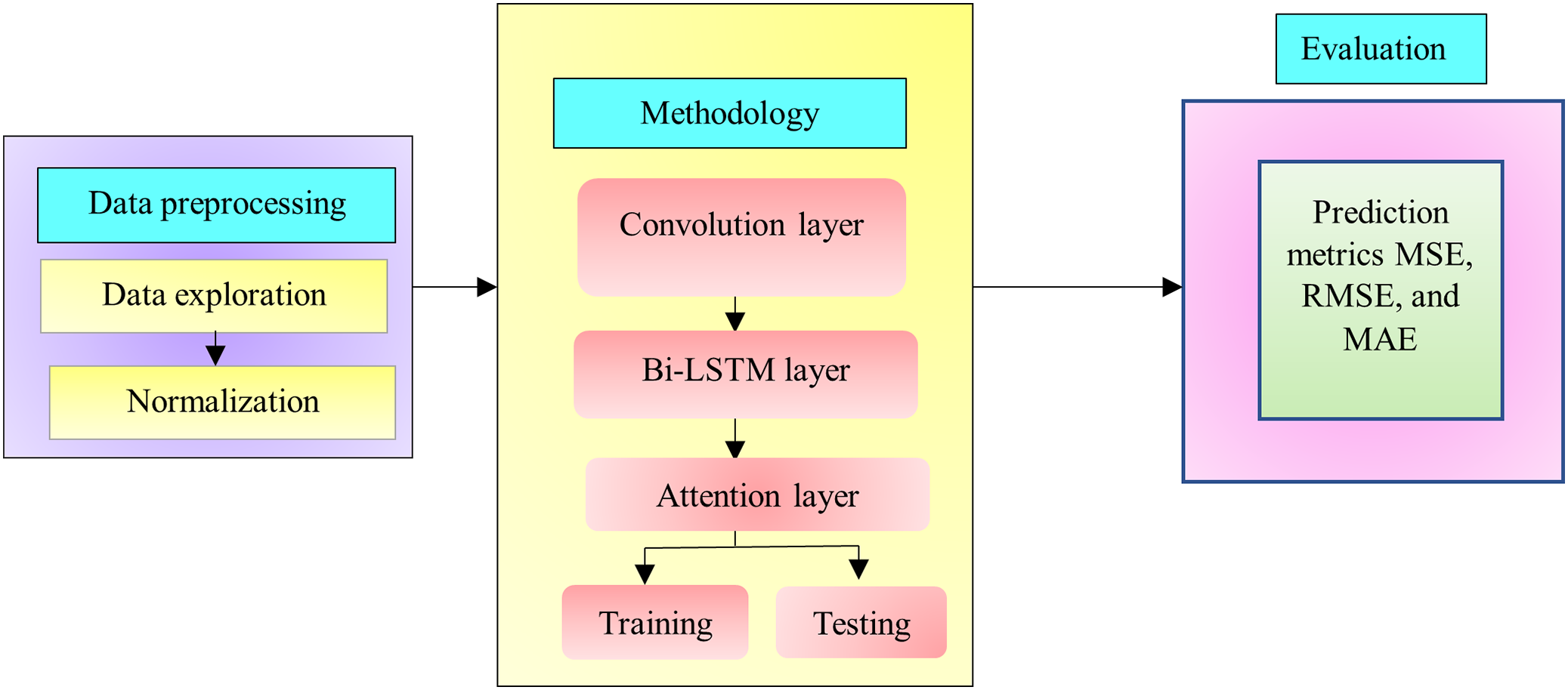
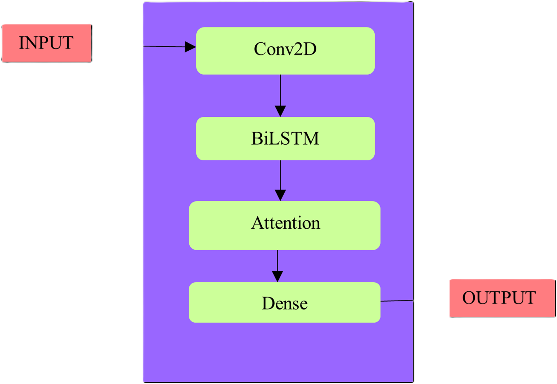
Improving transportation efficiency is the primary goal of TFP, which aims to deliver accurate as well as suitable information about future traffic flows. Ideally, a traffic model would be able to account for the nonlinearity and randomness of transportation traffic conditions. Several algorithms based on statistics or ML have enhanced the accuracy of traffic predictions. The process of feature learning, which identifies and chooses the best characteristic features from the past traffic flow data, is crucial for developing an effective traffic model. Traffic flow’s geographic and temporal features frequently display periodicity and correlation. This study proposes a model that utilizes DL to enhance TFP. Figure 1 illustrates the architecture of the proposed system for predicting network traffic. This has the ability to alleviate traffic congestion by shedding light on traffic patterns, which in turn may aid in the development of infrastructure to do away with the issue.
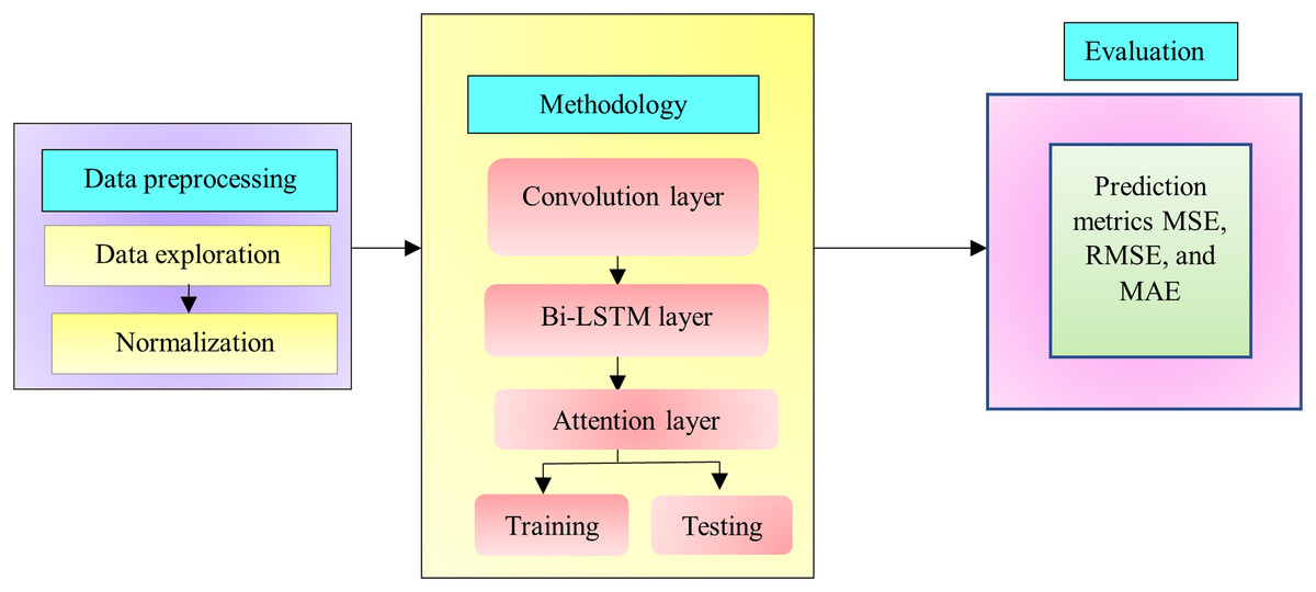
Figure 1: Proposed system architecture.
Dataset
Traffic congestion is increasing in cities worldwide. The increasing number of people living in cities, the aging infrastructure, the absence of real-time data, and the inefficiency and disorganization of traffic signal timing are all contributing factors. The effects are substantial. Thanks to wasted fuel, the improved cost of shipping products, lost time via congested regions, traffic congestion cost U.S. passengers an estimated $305 billion in 2017, according to data and analytics firm INRIX. Because there are budgetary and logistical constraints on constructing more roadways, cities must come up with innovative tactics and technology to alleviate traffic. This dataset includes 48,120 observations on the number of vehicles per hour at four distinct junctions, together with associated metadata such as datetime, junction, vehicles, and ID. The sensors at each intersection collected traffic data from distinct time periods. This should approach future predictions with caution due to the poor or restricted data supplied by some of the junctions (Kaggle, 2023).
This dataset consists of 48,120 observations across four distinct junctions (J1, J2, J3, J4). Each observation contains data on the number of vehicles per hour at a particular junction, along with additional metadata, such as datetime (timestamp), junction ID, and an ID for the data entry. The data was collected using sensors installed at each intersection over varying time periods. However, due to some missing or incomplete data from certain junctions, it is important to approach predictions with caution, particularly for junctions with poor data coverage or sensor malfunctions. The dataset is valuable for traffic prediction tasks in smart cities, where factors like traffic volume, weather conditions, and accident probability need to be considered. This dataset, help to understand traffic patterns, model congestion, and potentially forecast future traffic conditions.
Notably, Junction 4 includes segments of missing or sparse data. We conducted a sensitivity analysis by imputing missing values using time-aware interpolation (linear forward-fill based on temporal gaps). Post-imputation, we retrained the model and found that while overall RMSE slightly improved from 1.104 to 1.062, the overall ranking among models remained unchanged. These results suggest the model is robust to moderate missingness. Table 2 gives these details.
| Feature | Description | Details |
|---|---|---|
| Total entries | Number of observations in the dataset | 48,120 entries |
| Time period | Time range for data collection | Various time periods |
| Junctions | Number of junctions for which traffic data is recorded | 4 (J1, J2, J3, J4) |
| Traffic data | Type of traffic data collected for each observation | Number of vehicles per hour |
| Datetime | Timestamp for each data point indicating when the traffic data was collected | Yes (Date and time for each entry) |
| Junction ID | Unique identifier for each junction | Yes (e.g., J1, J2, J3, J4) |
| Vehicle count | Number of vehicles recorded at each junction during each time period | Yes (e.g., number of vehicles/hour) |
| Sensors | Type of sensors used to collect traffic data | Sensors at each junction |
| Metadata | Additional attributes or metadata associated with the traffic data | Junction ID, Datetime, etc. |
| Missing data | Note on data quality, such as gaps in data due to malfunctioning sensors or other issues | Some junctions have missing or incomplete data |
Feature engineering
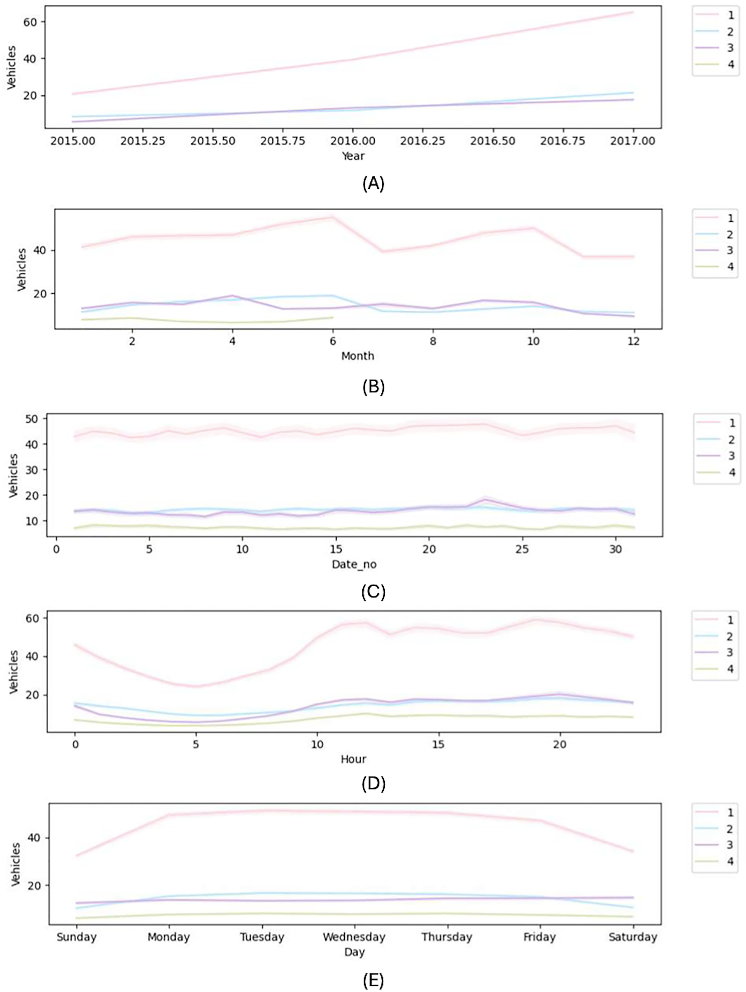
In order to create a traffic congestion detection system, this work propose a unique feature engineering approach that uses DL models. Using a proposed feature engineering framework, this work generates feature variables. The presentation of DL techniques will improve with excellent feature variables (Zhang, Wang & Liu, 2021). Currently, this study is developing new features based on DateTime data. The new features include year, month, date within the specified month, days of the week, and hour. Figure 2 displays all of these other features.
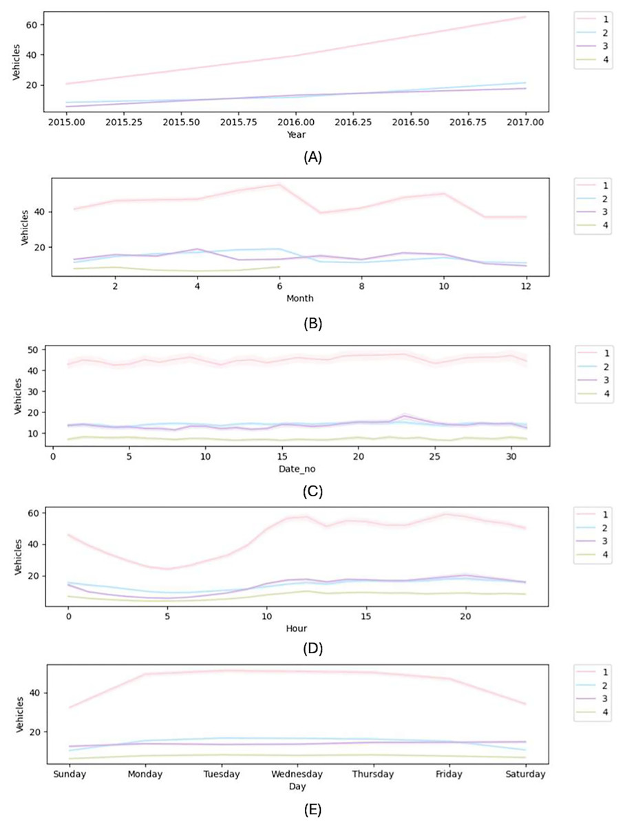
Figure 2: New features plot (A) year (B) month (C) date (D) hour (E) day.
Data preprocessing
This research presents the feature data on a large scale. This research hence normalized the data set to eliminate the influence of the feature scale. Normalization is a useful procedure to improve computational accuracy, prevent gradient explosions during network training, and hasten the loss function convergence. Equation (1) illustrates the computational process that occurs when it normalizes the data to [0, 1] employing Min-Max normalization.
(1)
The normalized value is denoted by ; the maximum as well as minimum values of the original data are and , respectively, and represents the original data. The flip-flop process denormalizes the output data, as it also normalizes the original data. Equation (2) shows the calculation formula.
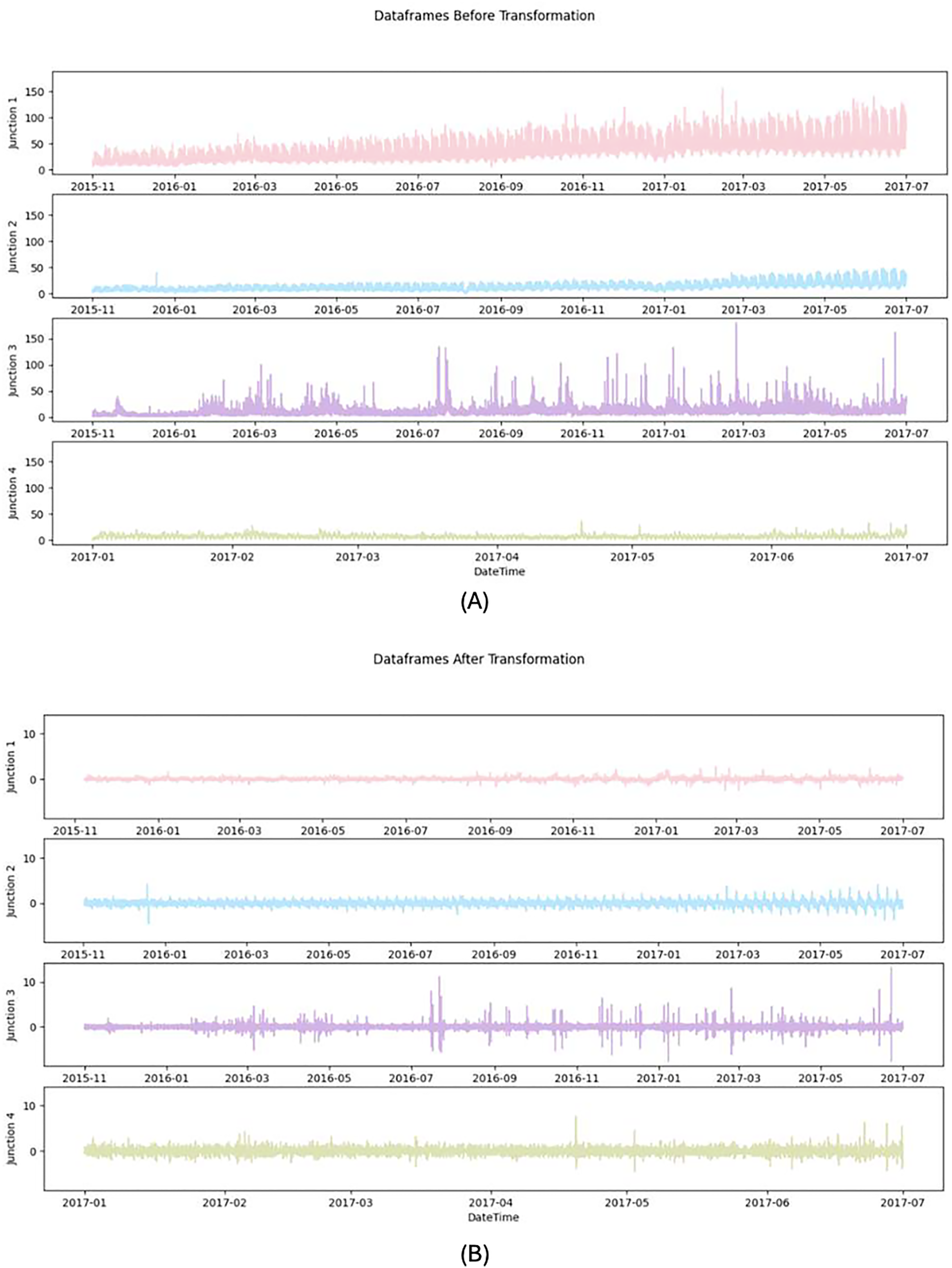
(2) where represents the predicted normalized traffic flow rate. The value of the actual prediction for the price of traffic flow, following denormalization, is represented by . Figure 3 shows the data frames before and after transformation.
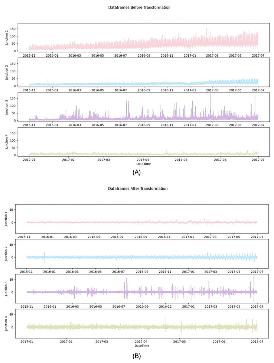
Figure 3: Dataframes (A) before preprocessing (B) after preprocessing.
Proposed attention based hybrid CNN with Bi-LSTM model
Convolutional neural network
The input to the CNN model is a univariate time-series vector, which represents the number of vehicles per hour at a junction over time. These sequences are reshaped into 1D arrays of fixed length (e.g., 32-time steps), allowing the CNN to extract local periodic trends. The fully connected, output layers, input, convolutional as well as pooling make up a CNN (Luo & Zhang, 2022). As a whole, the model relies on two layers—the convolutional and the pooling—to extract features and reduce their dimensionality. CNNs have proven useful in image and time series data classification due to their superior feature extraction. In order to gain more usable feature information, this study primarily focused on feature extraction utilizing pooling layer compression. It also successfully used convolutional layers to extract nonlinear local features from traffic flow data.
While CNNs are typically used for image-like data with explicit spatial dependencies, in this work, CNN is applied over 1D sequential data (time series of vehicle counts). CNN’s role is to detect local periodic trends—such as daily or weekly peaks—by capturing short-range temporal dependencies, similar to edge detection in image processing. These short-term directions serve as meaningful local features for Bi-LSTM to process later. This coordinates with recent works that utilize 1D CNNs to capture pseudo-spatial correlations in time-series domains such as stock price forecasting and energy consumption modeling.
Long short-term memory networks
Long-short-term memory (LSTM) neural networks outperform classic RNNs in areas such as predicting as well as processing critical events with long latency periods in time series (Wu et al., 2021). LSTM advances RNN’s hidden layer architecture by adding a gating unit system with input gates, forgetting gates, along with output gates. This fixes the gradient explosion as well as disappearance complications that happened while the model was being trained. Some of these gates include an input gate for updating the unit state, an output gate for controlling the output to the next neuron moment, and a forgetting gate for deciding which information in the model has to be erased from the neuron (Sun, Sun & Zhu, 2022). Here are the particular steps in Eqs. (3)–(8).
(3)
(4)
(5)
(6)
(7)
(8)
The outputs of the prior cell are denoted as and the present cell as . This represents the current unit’s inputs by . represents the current neuronal state. As part of the sigmoid activation function, the forgetting threshold indicates how the cell must dispose of outdated data. The input threshold determines which bits of data the sigmoid function must update, which, in turn, creates a fresh memory with the aid of the activation function and regulates the amount of new data included to the neural state. The output threshold , regulates the output neuron state of the sigmoid function, as well as the tanh activation function processes the neuron state to obtain the final result (Lu et al., 2020).
Here, the symbols , as well as , signify the input gate, the output gate as well as forgetting gate respectively. These gates’ weight coefficient matrices are , , and , and their offset constants are , , and , respectively. represents the neuron’s state, the hidden layer’s output, the Hadamard product along with the Sigmoid function.
Bidirectional long short-term memory neural network
Researchers (Xu, Wang & Wu, 2021) created an improved LSTM variant known as a Bi-LSTM neural network. Bi-LSTM connects the forward LSTM layer along with the backward LSTM layer, enabling the input of both forward as well as backward sequence data, thereby fully accounting for past and future data (Eapen, Bein & Verma, 2019). Using historical time series data, the classic LSTM can foretell the output at any given instant. Consequently, in order to extract bidirectional serial features from the CNN layer, this research deployed the Bi-LSTM neural network. Then fully utilized the long-term dependent characteristics of the sample data in learning process, along with the fully connected layer outputted the outcomes of traffic flow rate prediction. The formulas for each component of Bi-LSTM are provided below in Eqs. (9)–(11).
(9)
(10)
(11)
They correspond to the activation functions of layers , , and .
Attention mechanism
Research on the human visual system was the original source for the attention mechanism. When processing data, traditional neural networks do not discriminate between signals based on their relative relevance. Differentiated weight assignment can speed up the processing of information and stop the loss of information that happens during long sequences in LSTM. The attention approach can give dissimilar weights to dissimilar features at the same time. Consequently, the request of the attention mechanism may further enhance the accuracy of traffic flow rate predictions.
Other than the normally used attention layer this work creates a custom defined attention layer. This custom-defined attention layer across all junctions instead of relying on the predefined one. The task starts by deriving the Layer class and defining a new class called Attention. According to the rule for Keras custom layer creation, it is required to create four functions. The four functions are build(), call(), calculate_output_shape(), and get_config(). Define the biases and weights, and , within the build() method. The alignment scores are estimated as in Eq. (12):
(12) where , and is the hidden state at time step t. A softmax function is applied to and is termed in Eq. (13)
(13)
The result is a normalized weight and is called the attention weight. Also, the context vector c with a weighted average of hidden states is equated in Eq. (14).
(14)
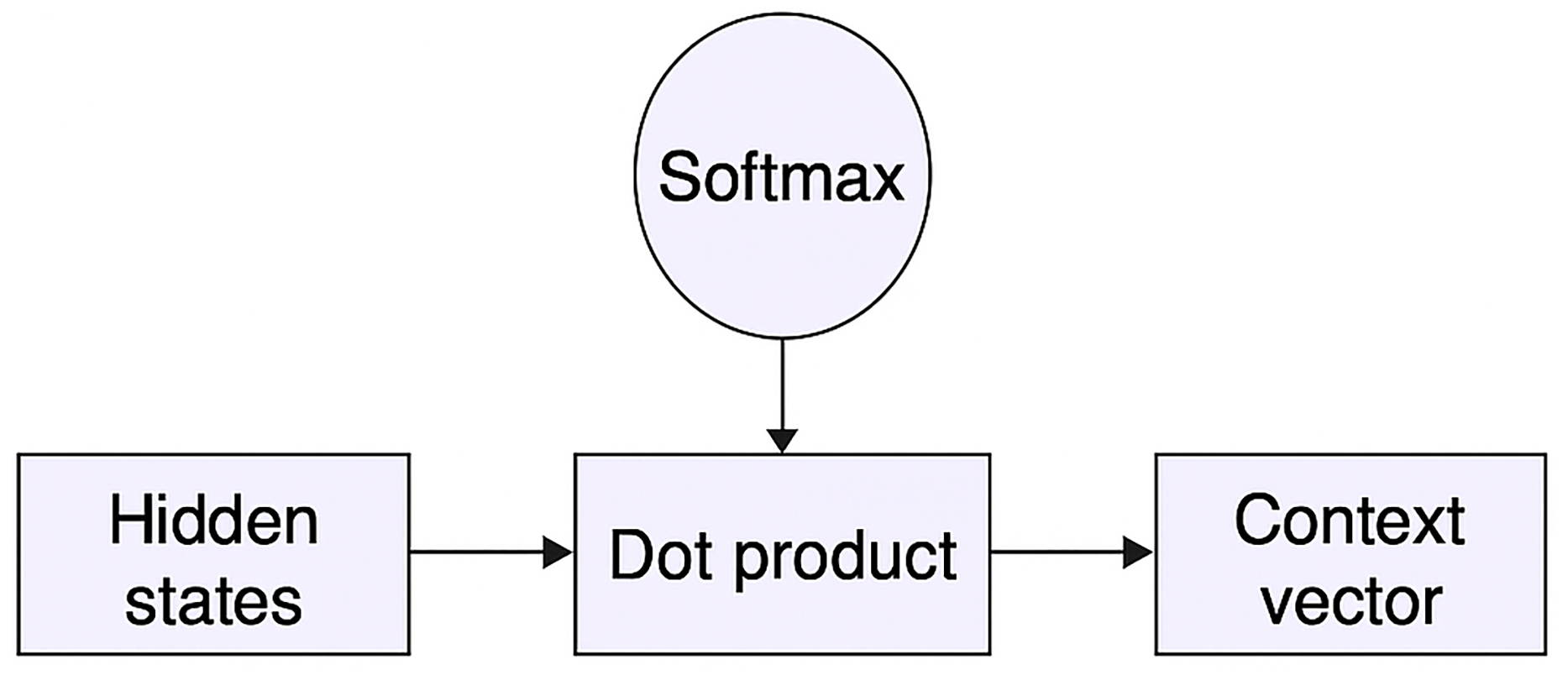
The is then passed to the dense output layer. With an output shape of (None, 32, 100) from the preceding LSTM layer, it should get a weight and bias of (100, 1) dimensions, respectively. Within the call() method, write the primary logic of Attention. It just needs to construct a multi-layer perceptron (MLP). To get the bias terms, this will first take the dot product of the inputs and weights and then add them. Next, apply a ‘tanh’ and a softmax layer. It gets the alignment scores from this softmax. It will have 32 dimensions, like the LSTM’s hidden states. This can obtain the context vector by taking the dot product of it and the hidden states. The get_config() function collects the input shape and other model-related data. Figure 4 depicts the custom attention mechanism.
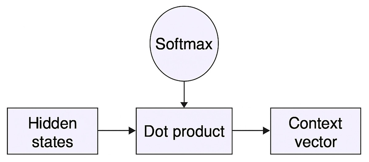
Figure 4: Custom attention mechanism.
Proposed method
The model input is a normalized time series of hourly traffic counts at specific junctions, where the output is the traffic flow predictions (vehicles/hour) for the next time interval. Each input sequence corresponds to a past window of 32 h, and the model predicts the immediate next hour’s traffic count. Prior discussion established that academics have attempted to utilize a change of methods to the critical problematic traffic flow forecasting, among others. Recent technological advancements may greatly improve prediction accuracy. This work thus proposes a CNN-Bi-LSTM based attention model, for TFP approach. Here is a detail of how this strategy works.
First things first, it normalized and split the gathered traffic flow data into testing and training sets. Initially, it used the pooling layer, dropout layer as well as 1D convolutional layer of the CNN to extract the intrinsic features of the traffic flow data. In order to train the Bi-LSTM layer to understand the underlying pattern of dynamic change, the CNN first extracted local features. The Bi-LSTM layer automatically assigned varied weights to the retrieved features to investigate the deep temporal correlation. Then included a custom attention mechanism for this purpose. The last step was to include a dense layer in the output. Figure 5 displays a diagram of its proposed network structure. Second, it normalized the prediction results to obtain the correct numbers.
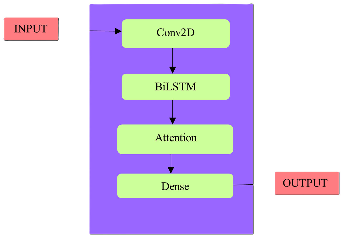
Figure 5: Proposed methodology architecture.
Results
The model was developed and executed using the Windows 11 operating system, Intel Core i5 processor and 16 GB RAM. The python version 3.9 is used in Jupyter Notebook utilizing TensorFlow and Keras. Other libraries such as NumPy, Pandas, Matplotlib, Seaborn, scikit-learn, etc., are also used. This work, built the attention-based Bi-LSTM model with the CNN model using the Jupyter environment Python. It uses ReLU as an activation function. This uses the mean squared error (MSE) function as the loss function. This specifically use the Adam optimization technique as the optimizer to revise the parameters of every network layer. The Adam optimizer is ready to go with a starting learning rate of 0.001, decay steps of 10,000, and decay rates of 0.9. The inclusion of the dropout layer, with a drop rate of 0.2, enhanced the model’s generalizability, training duration, and overfitting prevention. The model was trained using a fixed training-testing split for each junction that is 80% training and 20% testing. This approach reflects a traffic prediction where future data is not available during training. Although k-fold cross-validation was not applied due to the high training time and sequential nature of traffic data, the use of multiple junctions for evaluation and consistent test performance across models helps to ensure result robustness. This research also compares the built model’s prediction performance to that of GRU, LSTM, CNN, as well as MLP models to ensure the model’s efficacy.
Hyperparameter tuning
To validate the robustness of the proposed model, various hyperparameters were experimented with, including:
Learning rate: Tested values of 0.0001, 0.001, and 0.01
Batch size: Ranges from 32 to 128
Dropout rates: 0.2, 0.3, and 0.5
Number of Bi-LSTM units: 50, 100, 150
Number of filters in CNN: 32, 64, 128
After comparative analysis on validation RMSE, the selected configuration (CNN with 64 filters, Bi-LSTM with 100 units, dropout 0.2, learning rate 0.001) consistently showed the best generalization across all junctions.
Evaluation metrics
This work includes the different performance for evaluation such as the MAE, RMSE and MSE. The evaluation Eqs. (15)–(17) define the difference between the predicted and observed data.
(15)
(16)
(17)
When N is the total count of observations, are the estimated responses, as well as are the observed responses.
Table 3 displays the loss and validation loss for four distinct junctions. Normally, rather than the loss, validation loss will be considered. Since this work executes for 10 epochs the loss and validation loss are attained for nearly 10 epochs. Among them the loss and validation loss for three epochs are explained such as the first, fifth and tenth epoch. Junction 1 has a validation loss of 0.070 at 10 epochs, Junction 2 at 0.201, Junction 3 at 0.689, and Junction 4 at 0.678. While observing the table it is evident that the proposed model shows less validation loss than the other existing models.
| Junction | Model | Epoch | Loss | Validation loss |
|---|---|---|---|---|
| J1 | Proposed | 10 | 0.049 | 0.065 |
| BiLSTM-CNN (no attention) | 10 | 0.056 | 0.0738 | |
| GRU | 10 | 0.063 | 0.093 | |
| LSTM | 10 | 0.079 | 0.112 | |
| CNN | 10 | 0.057 | 0.077 | |
| MLP | 10 | 0.068 | 0.073 | |
| J2 | Proposed | 10 | 0.178 | 0.318 |
| BiLSTM-CNN (no attention) | 10 | 0.185 | 0.344 | |
| GRU | 10 | 0.203 | 0.415 | |
| LSTM | 10 | 0.274 | 0.718 | |
| CNN | 10 | 0.159 | 0.330 | |
| MLP | 10 | 0.201 | 0.074 | |
| J3 | Proposed | 10 | 0.268 | 0.347 |
| BiLSTM-CNN (no attention) | 10 | 0.277 | 0.365 | |
| GRU | 10 | 0.263 | 0.396 | |
| LSTM | 10 | 0.325 | 0.404 | |
| CNN | 10 | 0.267 | 0.361 | |
| MLP | 10 | 0.267 | 0.129 | |
| J4 | Proposed | 10 | 0.609 | 1.102 |
| BiLSTM-CNN (no attention) | 10 | 0.644 | 1.131 | |
| GRU | 10 | 0.759 | 1.243 | |
| LSTM | 10 | 0.674 | 1.246 | |
| CNN | 10 | 0.637 | 1.186 | |
| MLP | 10 | 0.716 | 0.122 |
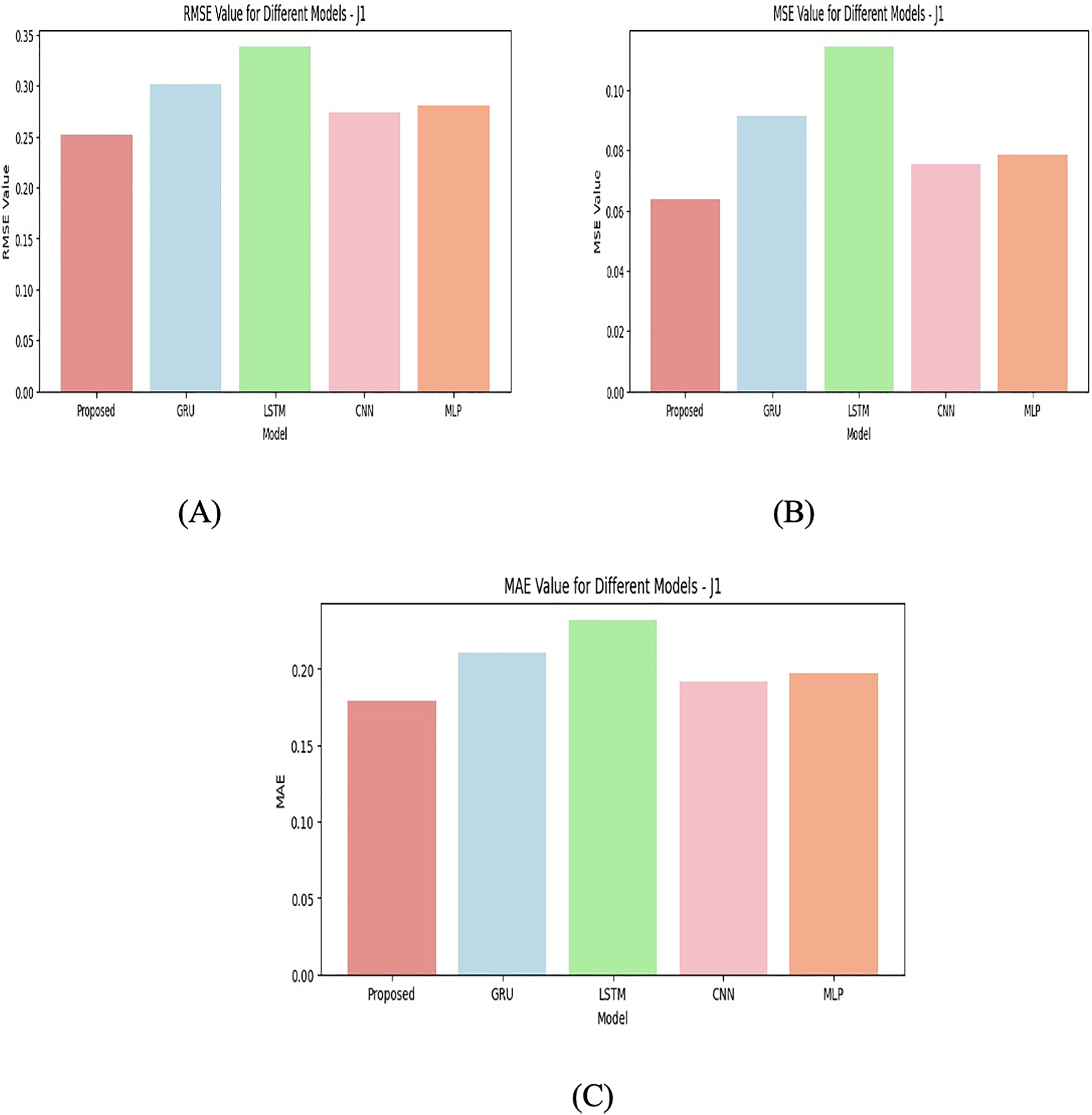
The performance of different ML models is compared including Proposed, GRU, LSTM, CNN, MLP on four junctions (J1, J2, J3, J4) using three performance metrics such as the RMSE, MSE, and MAE. To validate the effectiveness of the custom attention layer in the proposed hybrid architecture, an ablation study is also done. This process removes the attention mechanism and retrains the model with all four available junctions. The differentiation in results can be attributed to several factors including the nature of the model, the type of data, and the specific problem being solved. With J1 given in Fig. 6, the proposed model performs the best in terms of RMSE, MSE, and MAE compared to other models. It has the lowest error values, suggesting that the proposed model is well-suited to this particular junction’s data and task. Models like GRU, CNN, and MLP follow, with CNN having the second-best performance.
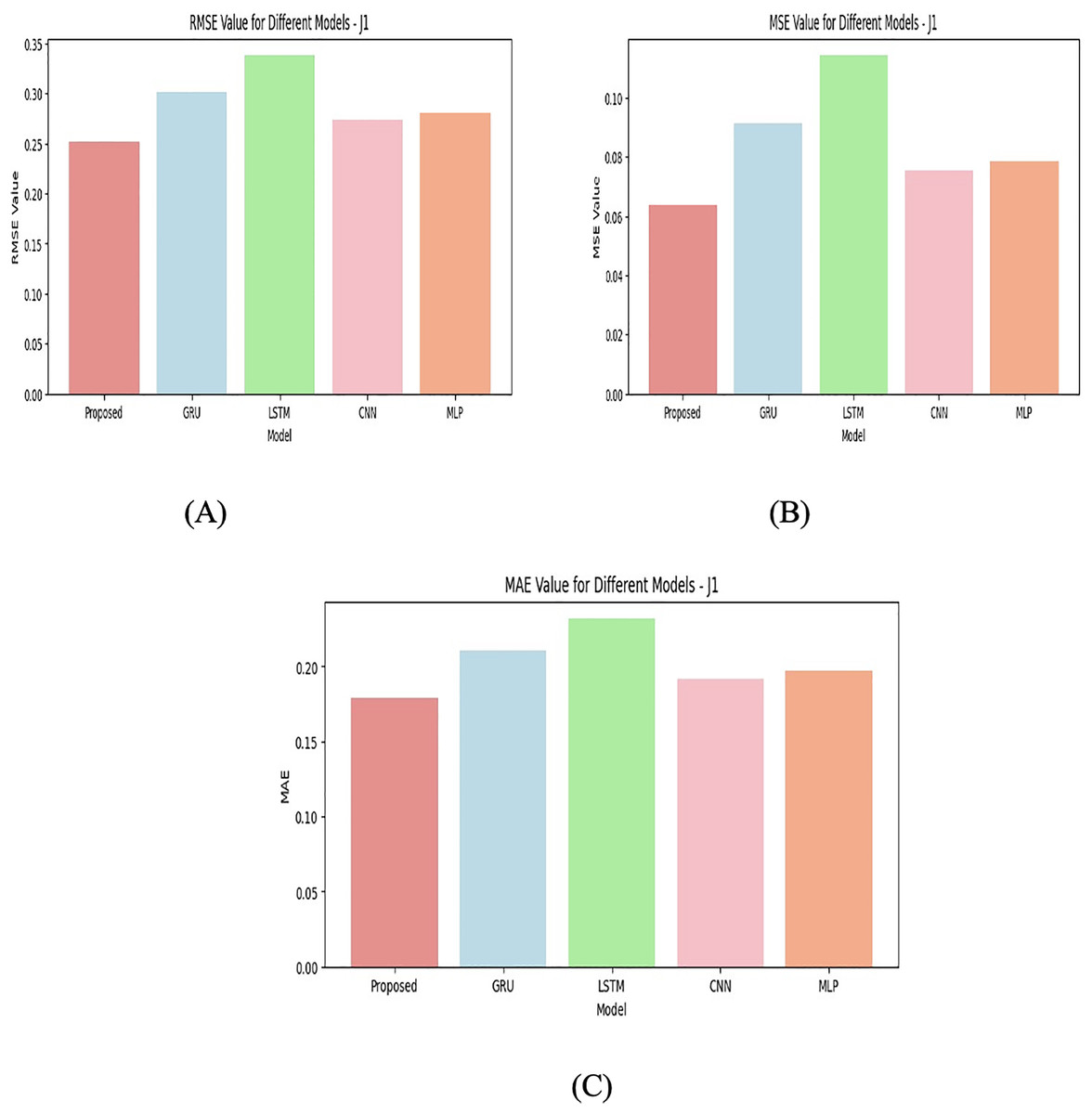
Figure 6: Junction 1 values for (A) RMSE (B) MSE (C) MAE.
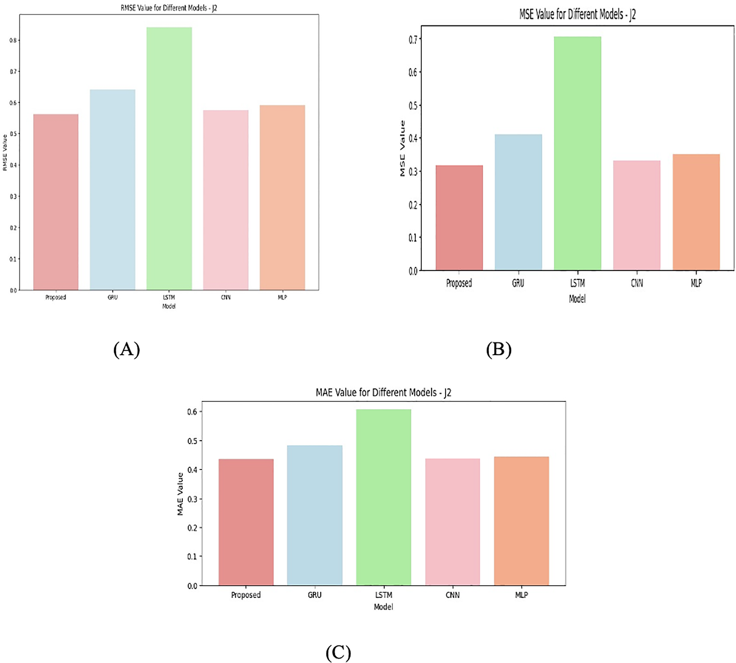
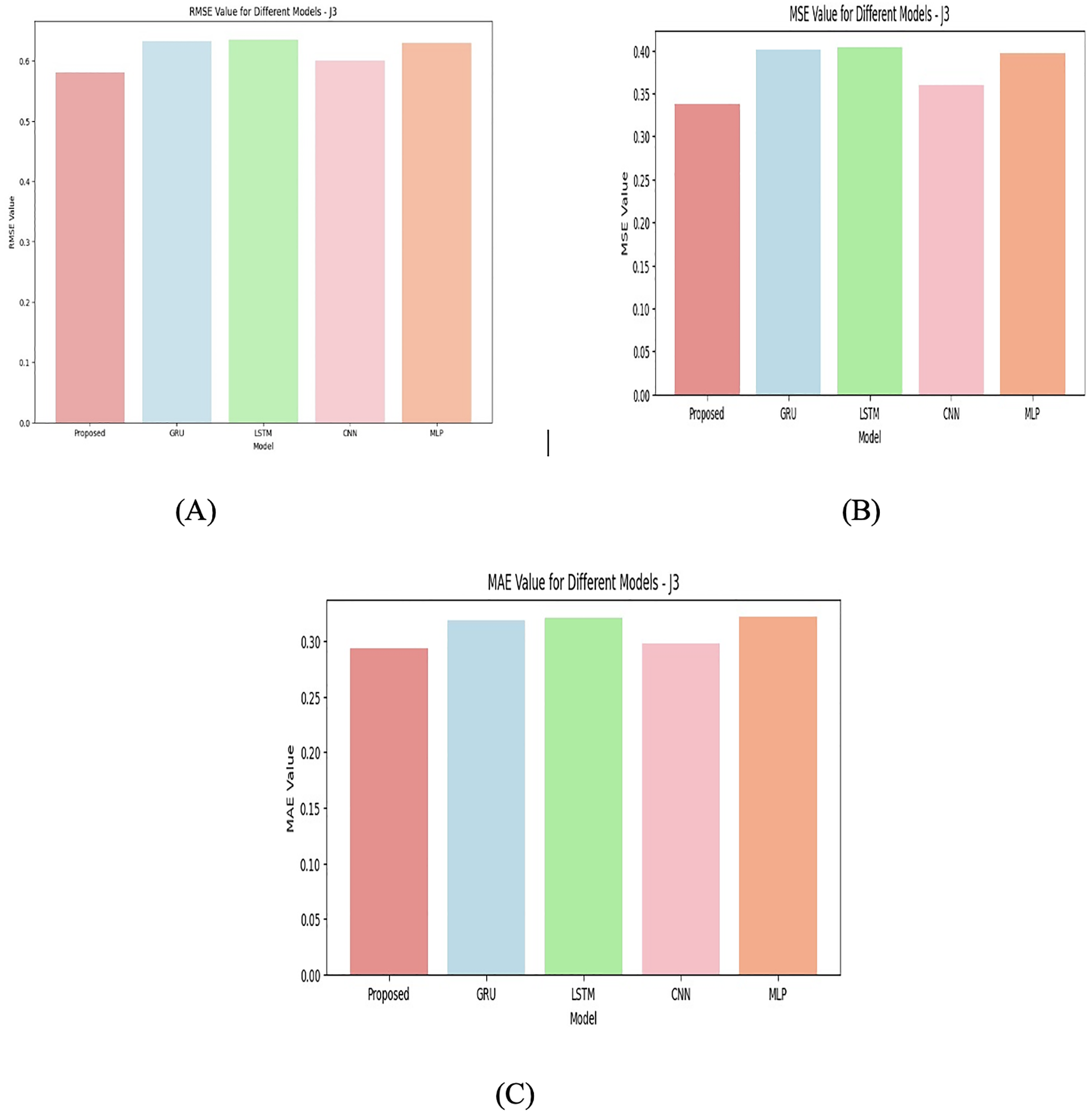
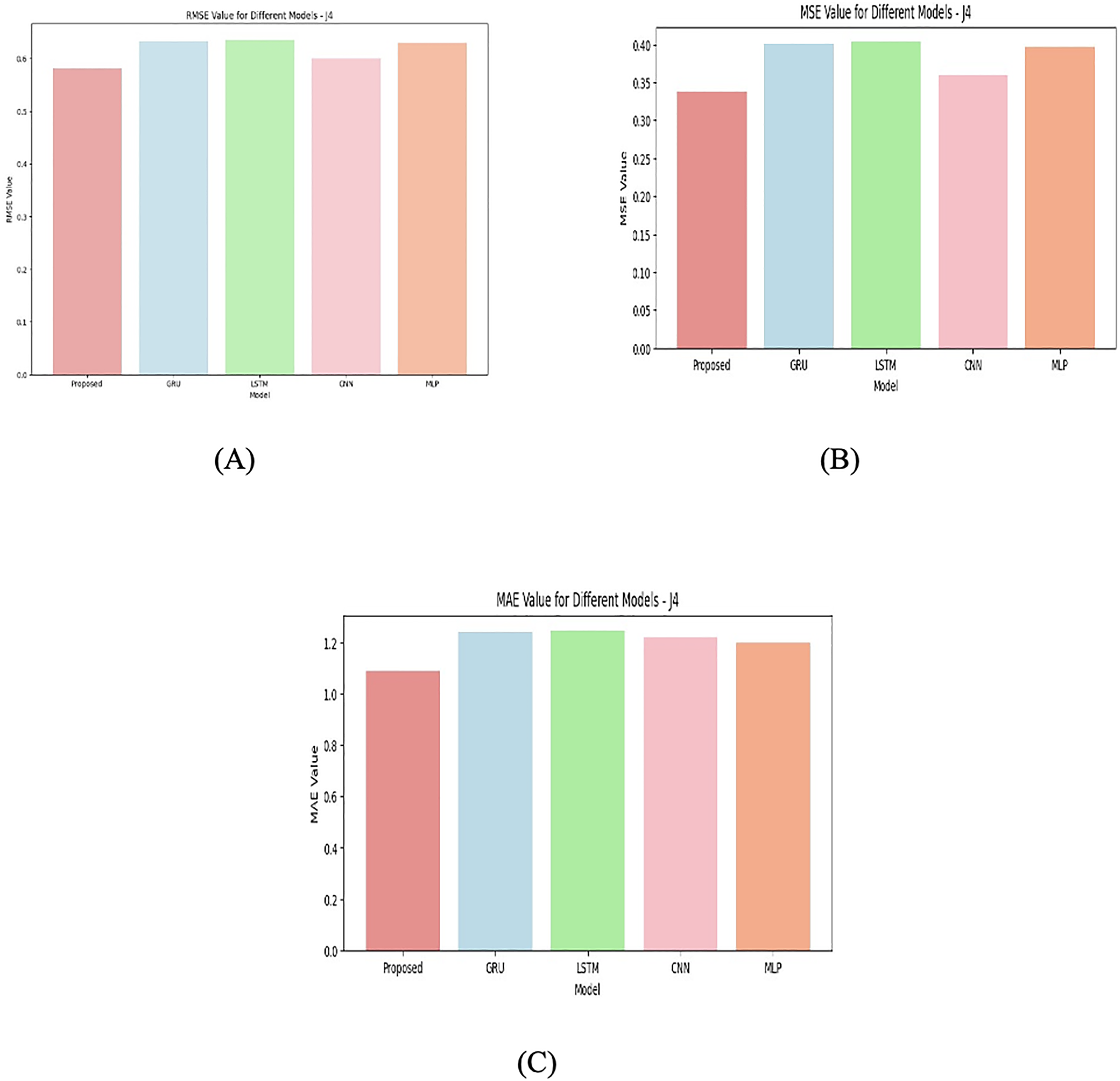
For J2 given in Fig. 7 the performance gap between models increases. The proposed model is still the best but has higher RMSE, MSE, and MAE values compared to J1. GRU follows closely behind, and LSTM performs the worst among the tested models. This could suggest that the data in J2 is more complex, requiring models like GRU that may capture temporal dependencies more effectively than LSTM in this case. Again, for J3 given in Fig. 8, the proposed model remains the best-performing model. The other models like GRU and LSTM perform similarly, with only minor differences in error metrics. It indicates that for J3 given in Fig. 9, the models capture patterns similarly, but the proposed model incorporate domain-specific knowledge. J4 junction has the highest error values across all models, with RMSE, MSE, and MAE all being significantly higher than in the other junctions. This suggests that J4’s data could be noisier, more complex, or more challenging to model, making accurate predictions harder. In this case, the proposed model is still the best, but the performance differences between models (GRU, LSTM, CNN, MLP) are more comparable. The higher error values reflect the models’ inability to adequately capture the patterns in the data of this junction.
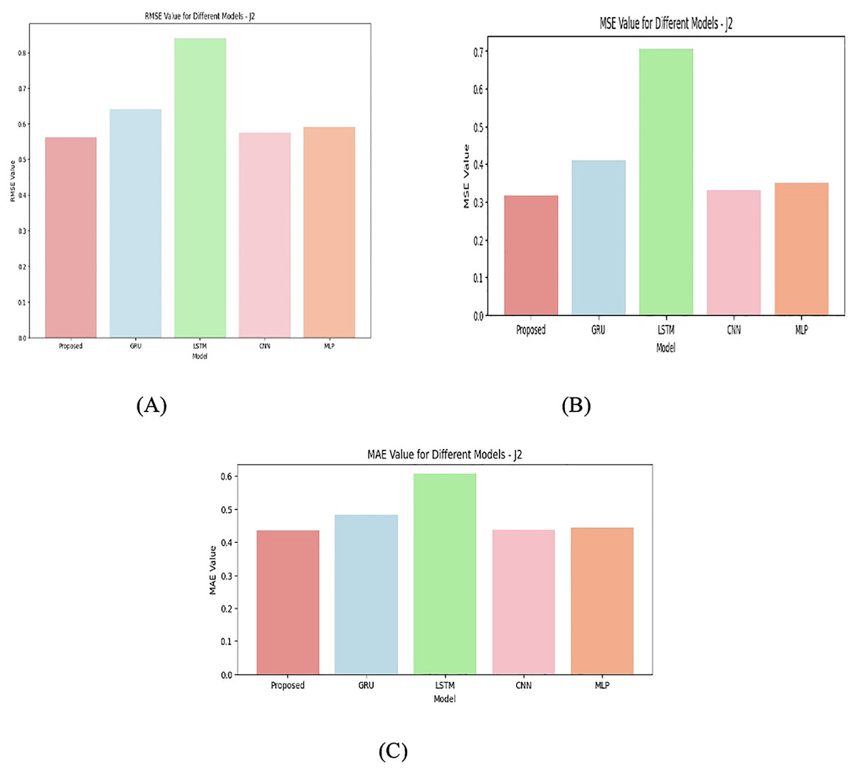
Figure 7: Junction 2 values for (A) RMSE (B) MSE (C) MAE.
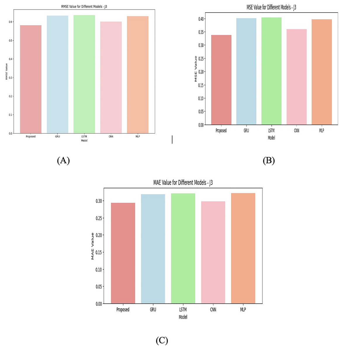
Figure 8: Junction 3 values for (A) RMSE (B) MSE (C) MAE.
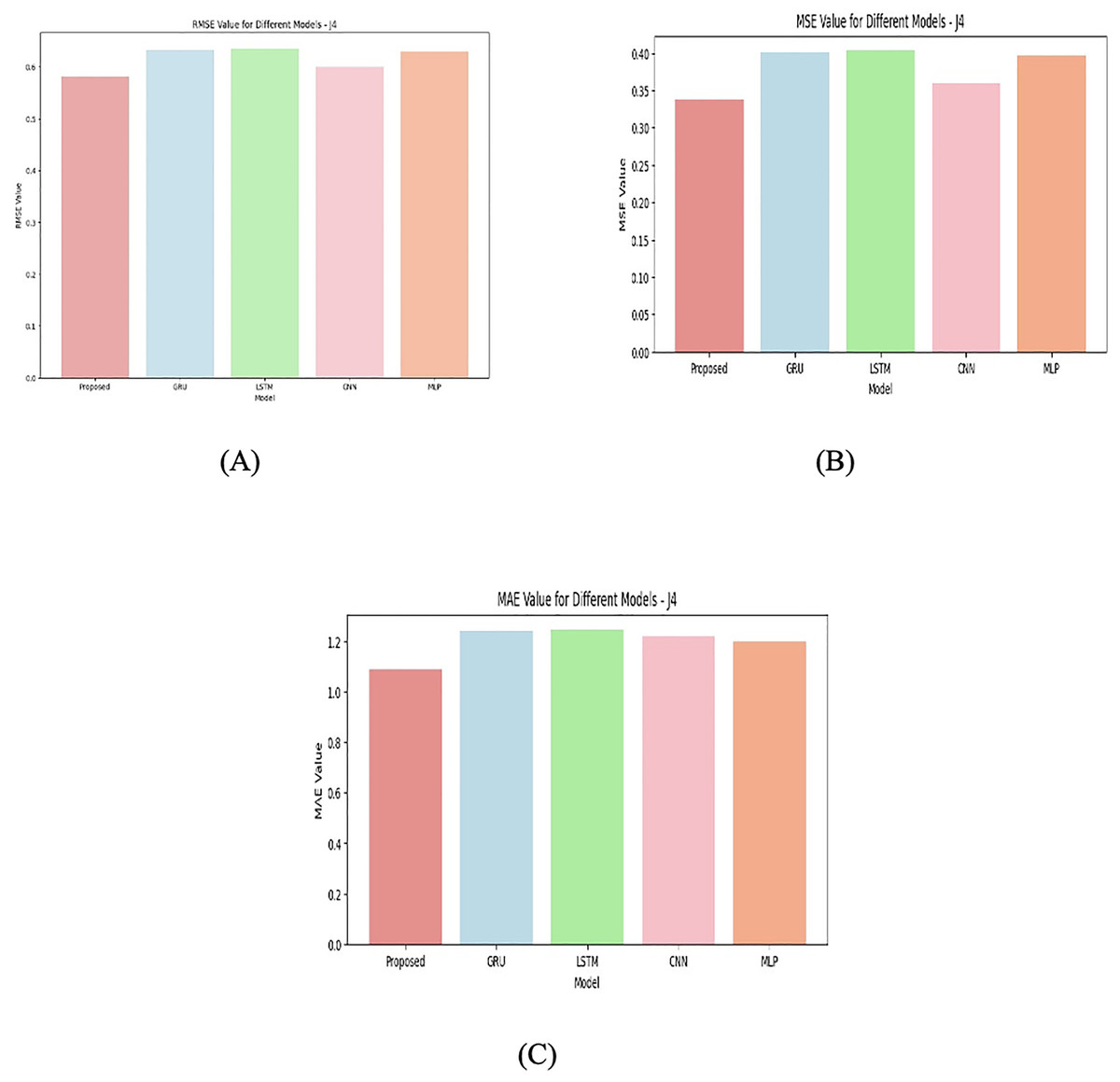
Figure 9: Junction 4 values for (A) RMSE (B) MSE (C) MAE.
The reason for this results differentiation comes first with data complexity. Each junction represents a different distribution of the data or different underlying patterns, and some models perform better on certain types of data. Second is the model type. GRU is generally effective for time-series data, GRUs can model sequential dependencies. They are often better at handling long-term dependencies than simpler models like CNN or MLP, especially when the data has time-series characteristics. Like GRU, LSTMs are designed to capture long-range dependencies, but they tend to be more complex and require more training data or hyperparameter tuning to perform optimally. In some junctions, LSTM may not perform as well due to overfitting or inadequate training.
CNNs are usually good at detecting spatial patterns, and in cases where the data is not strictly sequential, CNNs may outperform RNN-based models like GRU or LSTM. In J1, for example, CNN is quite close to GRU and proposed model, suggesting it is able to extract relevant features effectively. MLPs are versatile but is not be as good at handling sequential or temporal data unless they are specifically designed for such tasks. As seen in the table, MLP typically performs worse than GRU and LSTM, but better than CNN in certain junctions. Models like LSTM might suffer from overfitting or poor generalization if the junctions have high variability or noise, as seen in J4. Overfitting could lead to worse performance on the validation data despite good training results. On the other hand, simpler models like CNN or MLP may not have enough complexity to model intricate patterns, leading to underfitting in more complex junctions (like J4). J1 is simpler or more predictable, allowing models like GRU, CNN, and the proposed model to capture the patterns well. J2 and J3 might involve more complex relationships or dependencies, favoring models that can capture those patterns, such as GRU and LSTM. J4 likely represents the most challenging scenario with high levels of noise, non-linearity, or other factors that make it difficult for any model to generalize well, leading to higher errors across all models. The attention-based model consistently outperformed its non-attention variant in all three-performance metrics, confirming the usage of the attention layer in emphasizing relevant temporal features.
The proposed model seems to consistently outperform others, likely because it incorporates additional domain-specific features or architectures that improve its ability to handle the data from different junctions. GRU and LSTM generally perform well when the data has temporal dependencies, but their performance varies across junctions, indicating that some junctions are better suited for specific types of models. CNN performs competitively on some junctions, especially when the problem may involve feature extraction that is spatially correlated. The higher errors in J4 suggest that the junction’s data is more challenging, and none of the models is fully capable of accurately capturing the underlying patterns. Overall, the performance differentiation across the junctions is likely due to a combination of the complexity of the data in each junction and the inherent strengths and weaknesses of each model type in capturing those patterns. The four junctions for various models are shown in Figs. 6, 7, 8, and 9.
Discussions
Since the proposed model outperforms the other existing models, its prediction results are also visual. The actual results and the prediction results for every four models are illustrated in Fig. 10.
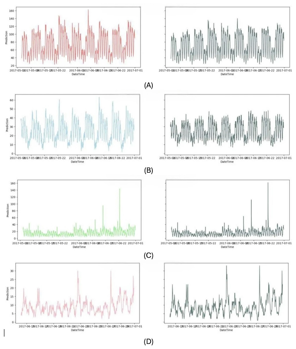
Figure 10: Proposed prediction results.
(A) junction 1 (B) junction 2 (C) junction 3 (D) junction 4.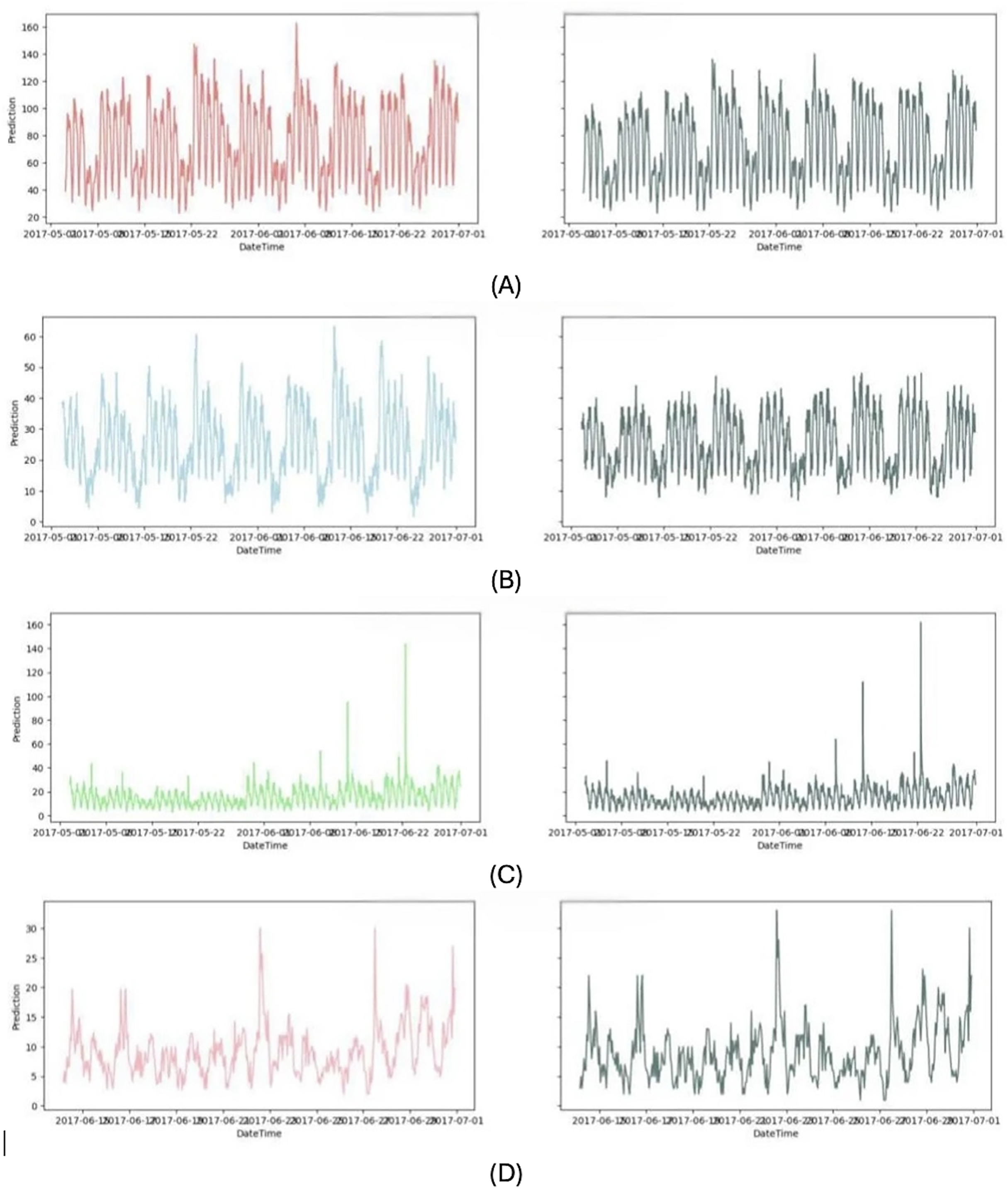
The proposed Attention based CNN with Bi-LSTM model performed better than the other four existing models, and the predicted values tracked variations in the observed values. A straight line connected the curves representing the accurate value and the prediction. Adding an attention mechanism to the CNN-LSTM model reduced its prediction impact even more, while the single LSTM model had the lowest overall effect. The reason for this is that the attention process enables the model to identify and isolate the crucial characteristics from a wide range of characteristics that significantly influence the predictions. The ablation experiment highlights that even a small improvement in prediction accuracy due to attention (~1.3% RMSE reduction) is meaningful. The attention mechanism used thus enhances model focus on critical time steps, improving temporal feature extraction in sequences. This is probably because the Bi-LSTM model fully makes use of the relationship between the forward as well as backward feature dimensions on the time series, allowing for the collection of more feature information and, therefore, enhancing the model’s prediction accuracy. Consequently, the proposed model achieved the best prediction effect.
Conclusion
This study, propose the CNN-Bi-LSTM-Attention model for traffic congestion prediction, aiming to reduce prediction loss. The model outperforms other state-of-the-art approaches, such as GRU, LSTM, CNN, and MLP, across key error metrics: RMSE, MSE, and MAE. For J1, the proposed model achieved the lowest RMSE of 0.252, MSE of 0.063, and MAE of 0.178, significantly outperforming GRU (RMSE = 0.302), LSTM (RMSE = 0.337), and CNN (RMSE = 0.274). In J2, the proposed model also led with an RMSE of 0.561 and MSE of 0.315, compared to GRU (RMSE = 0.640) and LSTM (RMSE = 0.839), demonstrating better generalization. Similarly, in J3, the proposed model had the best performance with RMSE of 0.580, while GRU and LSTM showed RMSEs of 0.632 and 0.634, respectively. In J4, where all models faced higher error rates, the proposed model again outperformed others with RMSE of 1.104, MSE of 1.090, and MAE of 1.090. These results confirm the effectiveness of the CNN-Bi-LSTM-Attention model in predicting traffic congestion, suggesting its potential for improving real-time traffic management. Future studies will include additional datasets to further validate these findings. In certain junctions, like Junctions 1 and 2, the proposed hybrid model works well, while in others, like Junction 4, it exhibits significant validation loss. This difference in performance could be caused by the quality of the data, the way traffic flows in some places, or the fact that traffic patterns at different intersections are naturally complicated.
So in the future, issues like traffic density, intersection shape, and local traffic signals will be considered as they pertain to individual junctions to see whether they are impacting performance. Also, domain-specific improvements will be considered to deal with the varied circumstances across junctions or more sophisticated data augmentation approaches to make the model adaptive.