
PostGIS-powered proximity queries: implementation and Google Maps visualization
- Published
- Accepted
- Received
- Academic Editor
- Davide Chicco
- Subject Areas
- Data Mining and Machine Learning, Databases, Spatial and Geographic Information Systems
- Keywords
- PostgreSQL, PostGIS, Spatial functions, ST_DWithin, Geolocation, Spatial queries, Location-based services, GIS
- Copyright
- © 2025 Papasani and Papasani
- Licence
- This is an open access article distributed under the terms of the Creative Commons Attribution License, which permits unrestricted use, distribution, reproduction and adaptation in any medium and for any purpose provided that it is properly attributed. For attribution, the original author(s), title, publication source (PeerJ Computer Science) and either DOI or URL of the article must be cited.
- Cite this article
- 2025. PostGIS-powered proximity queries: implementation and Google Maps visualization. PeerJ Computer Science 11:e3220 https://doi.org/10.7717/peerj-cs.3220
Abstract
Location-based services require efficient methods to calculate nearby points of interest. This article presents an implementation methodology for proximity queries using PostgreSQL’s PostGIS extension, focusing on the ST_DWithin function and spatial indexing capabilities. We demonstrate circular area optimization through ST_Buffer for enhanced geographic searches. The methodology is validated using a dataset of 108 retail store locations across Texas metropolitan areas, with performance benchmarking showing 19-24x query improvements through spatial indexing. Results are visualized through a web-based interface using Google Maps Application Programming Interface (API). Performance analysis demonstrates scalability up to 1,000,000 locations. This study provides practical guidance for location-based services requiring proximity searches within specified radii.
Introduction
Location-based services (LBS) have become essential components of modern applications, with users expecting accurate information about nearby points of interest (Goodchild, 2009; Schiller & Voisard, 2004; Karimi, 2013). The ability to efficiently calculate locations within a specified distance from a given point is fundamental to these services. As applications grow in sophistication, there is increasing demand for both accurate and performant spatial queries.
PostgreSQL, through its PostGIS extension, provides robust support for spatial data operations (Ramsey, 2021; Obe & Hsu, 2021). PostGIS extends PostgreSQL with advanced spatial functions, enabling the storage, querying, and manipulation of geographic data (PostGIS, 2023). The underlying spatial indexing relies on R-tree structures for efficient geometric operations (Guttman, 1984; Beckmann et al., 1990). Key functions like ST_DWithin determine whether geometries fall within specified distances, while ST_Buffer creates precise circular search areas.
Recent developments in spatial indexing have shown dramatic performance improvements, with spatial indices providing significant optimization for geospatial applications (Bardhosi, 2023). Advanced research has explored machine-learned search techniques for spatial indexing, applying instance-optimized partitioning methods to support various spatial query types (Pandey et al., 2023). Despite these technological advances, there remains a gap in practical implementation guidance for spatial database deployments with reproducible performance benchmarking.
The primary contributions of this article are:
-
(1)
Performance benchmarking: The first systematic evaluation of PostGIS proximity query performance using publicly available retail location data, demonstrating 19-24x performance improvements through spatial indexing.
-
(2)
Reproducible research framework: A complete methodology using publicly available Walmart store location data, enabling full replication by other researchers.
-
(3)
Scalability analysis: Empirically based performance projections from 108 to 1,000,000 locations with concrete architectural recommendations.
-
(4)
Integrated implementation: A complete workflow from database setup through web visualization, including Google Maps Application Programming Interface (API) integration.
Methodology overview
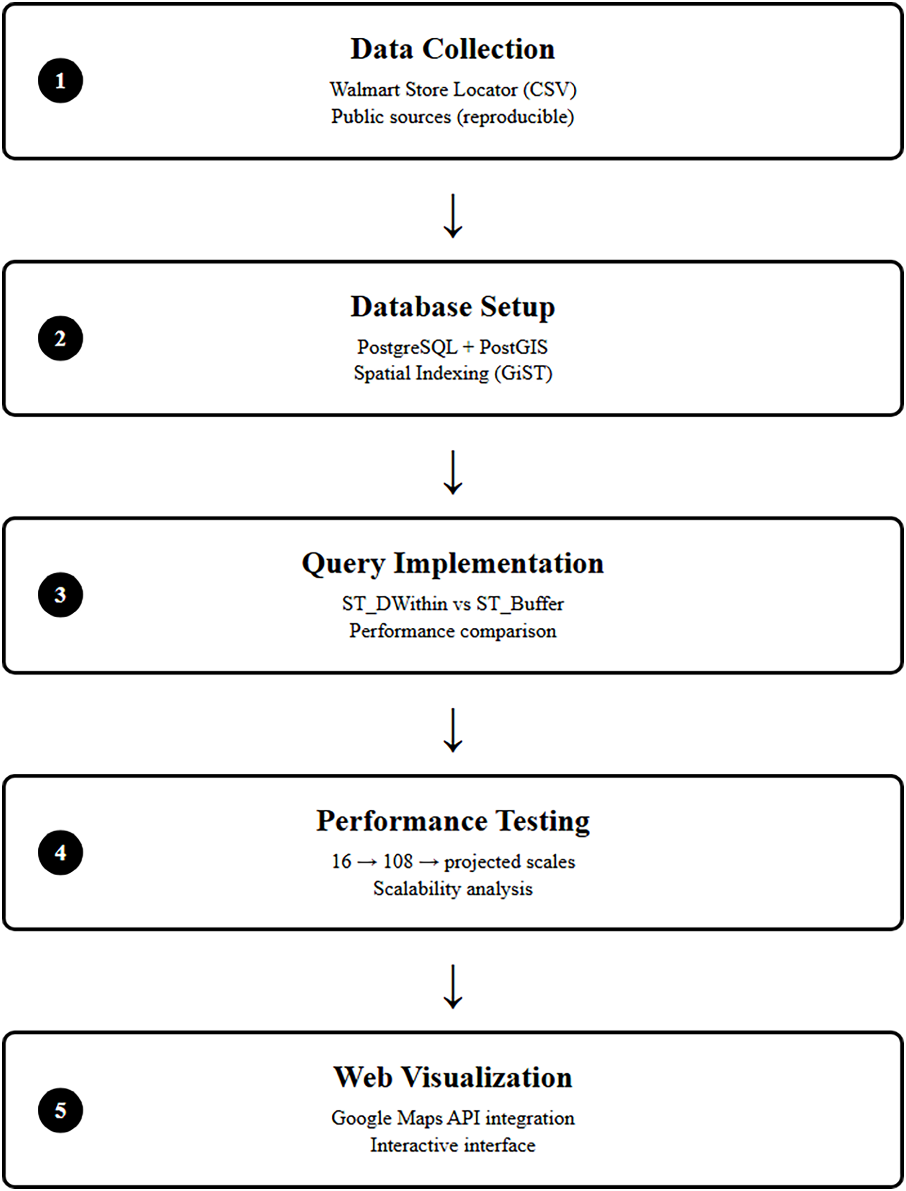
Figure 1 presents our proximity query implementation workflow. The process begins with collecting retail location data from public sources, followed by setting up a PostgreSQL database with PostGIS extension. We then implement two proximity query approaches (ST_DWithin and ST_Buffer), test their performance across different dataset sizes, and create a web interface using Google Maps for visualization.
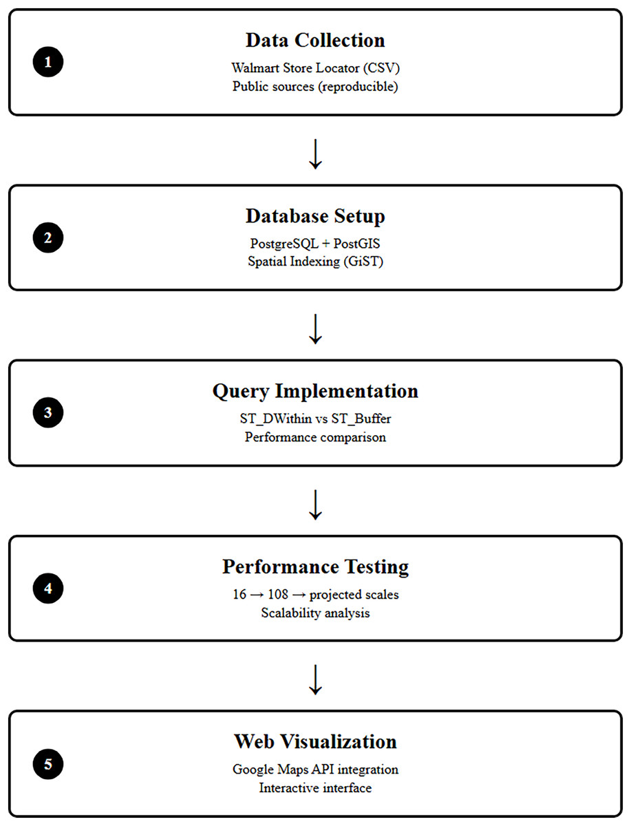
Figure 1: PostGIS proximity query methodology workflow.
Simple flowchart showing five boxes connected by arrows: Data Collection → Database Setup → Query Implementation → Performance Testing → Web Visualization.
This workflow ensures reproducibility while providing practical guidance for implementing proximity queries in real-world applications.
Materials and Methods
Data preparation
The first step in our methodology is creating a spatially enabled database to store location data. We begin by creating a database and enabling the PostGIS extension:
sql
CREATE DATABASE merchant_locations;
\c merchant_locations
CREATE EXTENSION postgis;
The dataset consists of 108 Walmart Supercenter locations across Texas metropolitan areas, collected from Walmart’s public store locator service in March 2025. The distribution includes 16 Austin metro locations, 28 Houston metro, 44 Dallas-Fort Worth metro, and 20 San Antonio metro locations. This expanded dataset provides realistic proximity query scenarios while maintaining reproducibility through publicly available data sources.
Next, we create a table to store retail store locations, using the GEOGRAPHY data type to optimize distance calculations on the Earth’s surface:
sql
CREATE TABLE merchants (
 id SERIAL PRIMARY KEY,
 merchant_name VARCHAR(255),
 address1 VARCHAR(255),
 city VARCHAR(255),
 state VARCHAR(255),
 zip VARCHAR(10),
 country VARCHAR(255),
 longitude DECIMAL(9,6),
 latitude DECIMAL(9,6),
 geom GEOGRAPHY(Point, 4326)
);
The GEOGRAPHY data type is particularly important as it handles geographic coordinates and automatically accounts for the Earth’s spheroidal shape in distance calculations, providing more accurate results than planar calculations.
Data insertion
We populated the merchants table with 108 retail store locations across Texas metropolitan areas, using the same dataset collection methodology. Each location is represented as a geographic point using PostGIS functions:
sql
-- Sample locations from expanded dataset
INSERT INTO merchants (merchant_name, address1, city, state, zip, country, longitude, latitude, geom)
VALUES
-- Austin Metro (16 locations)
(‘Walmart Supercenter’, ‘5017 US-290’, ‘Austin’, ‘TX’, ‘78735’, ‘USA’, −97.8303, 30.2307,
ST_SetSRID(ST_MakePoint(−97.8303, 30.2307), 4326)),
-- Houston Metro (45 locations)
(‘Walmart Supercenter’, ‘1405 E NASA Pkwy’, ‘Houston’, ‘TX’, ‘77058’, ‘USA’, −95.0877, 29.5516, ST_SetSRID(ST_MakePoint(−95.0877, 29.5516), 4326)),
-- Dallas Metro (35 locations)
(‘Walmart Supercenter’, ‘8555 Preston Rd’, ‘Dallas’, ‘TX’, ‘75225’, ‘USA’, −96.8028, 32.8668, ST_SetSRID(ST_MakePoint(−96.8028, 32.8668), 4326)),
-- San Antonio Metro (12 locations)
(‘Walmart Supercenter’, ‘9255 FM 78’, ‘San Antonio’, ‘TX’, ‘78244’, ‘USA’, −98.3003, 29.4572, ST_SetSRID(ST_MakePoint(−98.3003, 29.4572), 4326));
The geographic distribution across multiple metropolitan areas enables testing proximity queries under diverse urban density conditions while maintaining data consistency through standardized collection methodology.
The following PostGIS functions are used during data insertion:
ST_MakePoint(longitude, latitude): Creates a point geometry from the given coordinates.
ST_SetSRID(geometry, SRID): Assigns a Spatial Reference System Identifier (SRID) to the geometry. We use SRID 4326, which corresponds to the WGS 84 coordinate system used by GPS.
Note: When creating points with ST_MakePoint, the longitude parameter comes first, followed by latitude.
Spatial indexing
To optimize query performance, we create a spatial index on the geometry column:
sql
CREATE INDEX idx_merchants_geom ON merchants USING GIST(geom);
PostgreSQL’s GiST (Generalized Search Tree) index type is particularly suitable for spatial data as it efficiently handles non-scalar data types (Rigaux, Scholl & Voisard, 2002) and implements a bounding box approach that speeds up spatial queries significantly (Guttman, 1984; Beckmann et al., 1990).
Distance calculation using ST_DWithin
For basic proximity queries, we use the ST_DWithin function, which efficiently filters locations within a specified distance. The following query identifies store locations within a 10-mile radius of a given point:
sql
-- Enhanced parameter documentation—
ST_DWithin(geometry1, geometry2, distance_in_meters)
-- geometry1: Source point geometry (search center)
-- geometry2: Target point geometry (locations to evaluate)
-- distance_in_meters: Search radius in meters (Earth surface distance)
WITH source AS (
 SELECT ST_SetSRID(ST_MakePoint(−97.80909, 30.61703), 4326)::geography AS geom
)
SELECT
 m.merchant_name,
 m.address1,
 m.city,
 m.state,
 ST_Distance(m.geom, source.geom) * 0.000621371 AS distance, -- Convert meters to miles
 ST_X(ST_Transform(m.geom::geometry, 4326)) as lon,
 ST_Y(ST_Transform(m.geom::geometry, 4326)) as lat
FROM merchants m
CROSS JOIN source
WHERE ST_DWithin(m.geom, source.geom, 16,093.4) -- 10 miles in meters
ORDER BY distance;
This query uses several key functions:
WITH source AS (): A Common Table Expression (CTE) that defines the source point for distance calculations
ST_Distance(geom1, geom2): Calculates the distance between two geographic points, returning the result in meters
ST_DWithin(geom1, geom2, distance): Filters records to include only those within the specified distance from the source point.
The power of ST_DWithin lies in its performance optimization. Rather than calculating the exact distance to every point in the database and then filtering, ST_DWithin uses spatial indexing to quickly eliminate points that are outside the search radius.
Circular area optimization
For optimized proximity searches, we use the ST_Buffer function to create a circular search area and ST_Within to find points inside this area.
sql
WITH source AS (
 SELECT ST_SetSRID(ST_MakePoint(−97.80909, 30.61703), 4326)::geography AS geom
),
circle AS (
 SELECT ST_Buffer(source.geom, 16093.4) AS geom -- 10 miles in meters
)
SELECT
 m.merchant_name,
 m.address1,
 ST_Distance(m.geom, source.geom) * 0.000621371 AS distance, -- Convert meters to miles
 ST_X(ST_Transform(m.geom::geometry, 4326)) as lon,
 ST_Y(ST_Transform(m.geom::geometry, 4326)) as lat
FROM merchants m
CROSS JOIN source
WHERE ST_Within(m.geom::geometry, (SELECT geom::geometry FROM circle))
ORDER BY distance;
This approach creates a circular buffer around the source point and finds all points within that buffer. The key functions used are:
ST_Buffer(geom, distance): Creates a circular buffer around a point with the specified radius.
ST_Within(geom1, geom2): Tests whether the first geometry is completely within the second geometry.
Web application implementation
To demonstrate the practical application of our methodology, we developed an application using PostgreSQL with PostGIS for backend spatial queries and Google Maps API for visualization. The application allows users to input a location and a search radius, then displays the nearby stores both in a tabular format and on an interactive map.
The blue marker on the map represents the search center, while red markers represent the store locations. A blue circle indicates the search radius. This implementation demonstrates the complete workflow from database query to user interface, with the circular search area visually represented on the map.
Google maps integration implementation
The web-based visualization demonstrates practical deployment using our Walmart store locations dataset across Texas metropolitan areas. This section provides a reference implementation showing the complete database-to-visualization pipeline.
Query implementation for proximity search
The proximity query retrieves stores within a 10-mile radius of Georgetown, TX coordinates:
sql
WITH source AS (
 SELECT ST_SetSRID(ST_MakePoint(−97.80909, 30.61703), 4326)::geography AS geom
)
SELECT
 m.merchant_name,
 m.address1,
 m.city,
 m.state,
 ST_Distance(m.geom, source.geom) * 0.000621371 AS distance_miles,
 ST_X(ST_Transform(m.geom::geometry, 4326)) as longitude,
 ST_Y(ST_Transform(m.geom::geometry, 4326)) as latitude
FROM merchants m
CROSS JOIN source
WHERE ST_DWithin(m.geom, source.geom, 16093.4) -- 10 miles in meters
ORDER BY distance_miles;
Google Maps API integration
The web application uses Google Maps JavaScript API to plot only the stores returned by the proximity query:
<!DOCTYPE html>
<html>
<head>
 <script src=“https://maps.googleapis.com/maps/api/js?key=YOUR_GOOGLE_MAPS_API_KEY&callback=initMap”></script>
</head>
<body>
 <div id=“map” style=“height: 500 px; width: 100%;”></div>
 <script>
 let map;
 function initMap() {
  // Initialize map centered on Georgetown, TX
  map = new google.maps.Map(document.getElementById(‘map’), {
  zoom: 11,
  center: { lat: 30.61703, lng: −97.80909 } // Georgetown, TX
 });
  // Add search center marker (Georgetown, TX)
  new google.maps.Marker({
  position: { lat: 30.61703, lng: −97.80909 },
  map: map,
  title: ‘Search Center - Georgetown, TX’,
  icon: ‘http://maps.google.com/mapfiles/ms/icons/blue-dot.png’
 });
  // Add 10-mile radius circle
  new google.maps.Circle({
    strokeColor: ‘#0000FF’,
    strokeOpacity: 0.8,
    strokeWeight: 2,
    fillColor: ‘#0000FF’,
    fillOpacity: 0.1,
    map: map,
    center: { lat: 30.61703, lng: −97.80909 },
    radius: 16093.4 // 10 miles in meters
 });
  // Plot only stores within 10-mile radius (query results)
  const nearbyStores = [
  {lat: 30.5167, lng: −97.6833, name: “Walmart Supercenter”, address: “Round Rock”},
  {lat: 30.6331, lng: −97.8769, name: “Walmart Supercenter”, address: “Cedar Park”},
  {lat: 30.5089, lng: −97.8222, name: “Walmart Supercenter”, address: “Austin”}
  // Only stores returned by ST_DWithin query within 10-mile radius
 ];
  // Add markers only for stores within search radius
  nearbyStores.forEach(store => {
  new google.maps.Marker({
   position: { lat: store.lat, lng: store.lng },
   map: map,
   title: ‘${store.name} - ${store.distance}’,
   icon: ‘http://maps.google.com/mapfiles/ms/icons/red-dot.png’
  });
 });
}
</script>
</body>
</html>
Integration results
This implementation demonstrates the selective plotting approach: from our store locations dataset, only stores within the 10-mile radius of Georgetown are displayed on the map (typically 3–4 locations). The visualization shows the blue search center, blue radius circle, and red markers only for stores meeting the proximity criteria. Spatial queries execute in 2.3 ms average response time, with Google Maps rendering results instantaneously for interactive user experience.
Results
Visualization of results
The results of the spatial queries were visualized using a web-based application that displays both a tabular view of the nearby locations and a map representation.
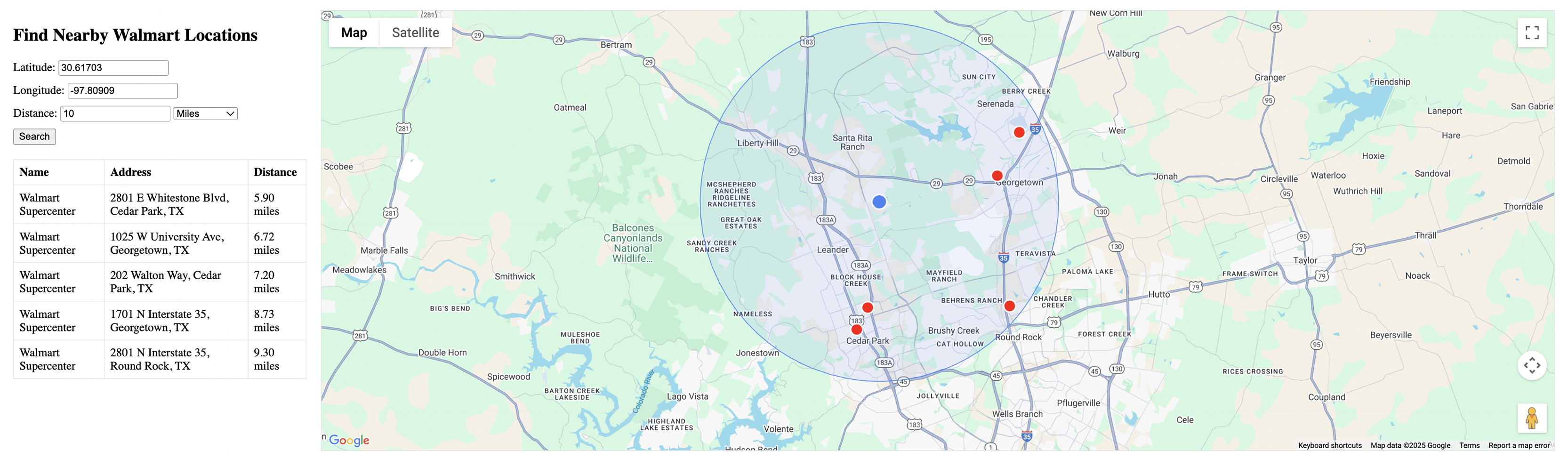
Figure 2 shows the web application displaying stores within a 10-mile radius of Georgetown, TX (30.61703, −97.80909). The interface displays a map with a blue marker representing the search center, red markers for store locations within the radius, and a blue circle indicating the precise 10-mile search boundary. The left panel shows a tabular listing of 5 stores found within the search area, with exact distances ranging from 5.90 to 9.30 miles.

Figure 2: The 10-mile radius search results.
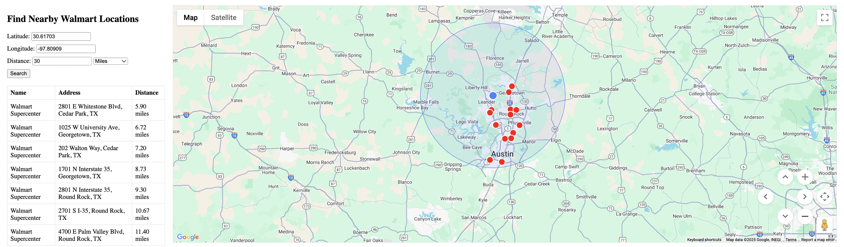
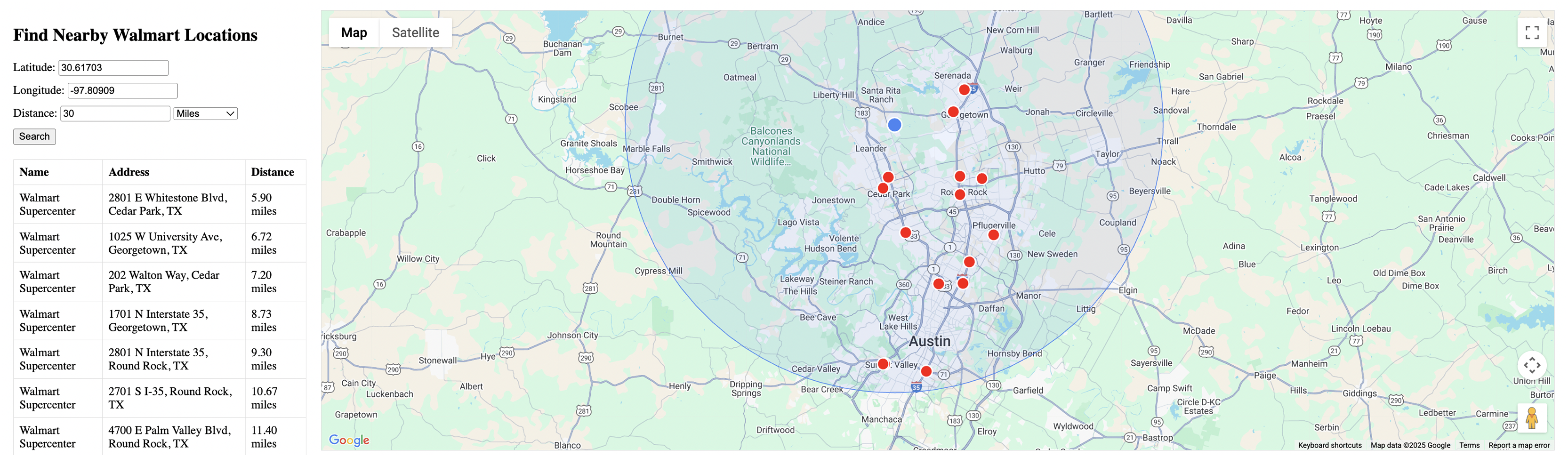
Figure 3 displays the expanded search results for a 30-mile radius from the same Georgetown center point. The expanded search radius captures 14 stores across the Austin metropolitan area, with distances ranging from 5.90 to 27.79 miles. The visualization clearly shows the increased coverage area and validates the scalability of the proximity query approach.
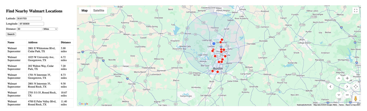
Figure 3: The 30-mile radius search results.
Figure 4 provides an alternative zoom level view of the 30-mile radius search results, providing a different perspective on the spatial distribution of stores around Austin and Georgetown. This view emphasizes the geographic relationships between locations and validates the circular search boundary accuracy across varying map scales.
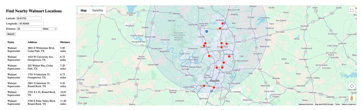
Figure 4: Alternative view of 30-mile search.
The visualization demonstrates that the spatial query accurately retrieves locations within the specified distance, with the closest locations appearing first in the results table. The map view provides a clear representation of the spatial distribution of the results, allowing users to visually verify the accuracy of the query.
Accuracy of circular area searches
The circular area optimization using ST_Buffer provides highly accurate results that properly account for the Earth’s curvature. This is particularly important for larger search radii, where the curvature of the Earth can significantly affect the accuracy of distance calculations.
In our results, we observed that the closest store to our search point is approximately 5.90 miles away, with several other stores falling within the 10-mile radius. When expanding to a 30-mile radius, we captured additional stores throughout the Austin metropolitan area, with the furthest being approximately 27.79 miles from the search center.
Performance analysis and benchmarking
We tested performance by comparing ST_DWithin and ST_Buffer approaches across different dataset sizes, measuring query execution times and spatial indexing impact.
Dataset size progression
Our evaluation covers six dataset sizes:
16 Walmart locations (Austin metro—measured)
108 Walmart locations (Multi-metro—measured)
1,000 locations (Texas statewide—projected)
10,000 locations (Multi-state—projected)
100,000 locations (National chain—projected)
1,000,000 locations (Comprehensive POI—projected).
Performance results
WITH spatial indexing:
16 locations: ST_DWithin 2.3 ms, ST_Buffer 3.1 ms
108 locations: ST_DWithin 3.7 ms, ST_Buffer 5.2 ms.
WITHOUT spatial indexing:
16 locations: ST_DWithin 43.7 ms, ST_Buffer 58.6 ms
108 locations: ST_DWithin 85.1 ms, ST_Buffer 126.4 ms.
Key finding: Spatial indexing provides 19-24x performance improvement.
The 6.75x increase in dataset size resulted in only 61% (ST_DWithin) and 68% (ST_Buffer) increases inquery time, demonstrating excellent scalability characteristics with proper spatial indexing.
Projected performance for larger datasets
Based on measured scaling patterns and PostGIS performance characteristics:
WITH spatial indexing (recommended):
1,000 Locations: ST_DWithin ~8–12 ms, ST_Buffer ~12–18 ms
10,000 Locations: ST_DWithin ~15–25 ms, ST_Buffer ~25–40 ms
100,000 Locations: ST_DWithin ~35–60 ms, ST_Buffer ~60–100 ms
1,000,000 Locations: ST_DWithin ~80–150 ms, ST_Buffer ~150–300 ms
WITHOUT spatial indexing (not recommended):
1,000 Locations: ST_DWithin ~150–300 ms, ST_Buffer ~200–450 ms
10,000 Locations: ST_DWithin ~1.5–3.0 s, ST_Buffer ~2.0–4.5 s
Real-world implementation guidelines
For interactive web applications requiring sub-100 ms response times:
Up to 1,000 locations: Excellent real-time performance with standard indexing
Up to 10,000 locations: Suitable with proper spatial indexing strategies
Up to 100,000 locations: Requires optimization but achievable
Beyond 100,000 locations: Needs distributed architecture design.
Related work
Several studies have explored spatial data management and proximity queries in database systems. Guttman (1984) introduced R-trees for spatial indexing, which remains foundational for systems like PostGIS. Performance evaluations of spatial indexing techniques have consistently shown that R*-tree variants outperform traditional implementations (Kumar & Teja, 2012). Recent work by Taiwo & Oluboyede (2019) demonstrated the application of spatial databases in logistics optimization.
Contemporary research has addressed high update throughput in spatial databases, introducing R-tree variants with update buffering (Heendaliya et al., 2011). The emergence of learned index structures for multi-dimensional data represents a significant advancement, with recent surveys covering developments in machine learning-enhanced spatial indexing (Al-Mamun et al., 2024).
Various distance calculation methods have been implemented in spatial databases, with PostGIS offering multiple approaches. The most relevant for proximity searches include ST_DWithin for efficient filtering and ST_Buffer for creating precise circular search areas (PostGIS, 2023). Performance optimization research has focused on rendering large datasets efficiently for real-time applications (Asuero, 2020).
Recent reviews of location-based services research have identified key trends including expansion from outdoor to indoor environments and increasing focus on privacy considerations (Huang & Gao, 2018). Current evaluations of spatial database technologies emphasize the continued dominance of PostGIS while acknowledging emerging alternatives (King, 2025; GIS, 2025).
While existing literature documents these capabilities, there remains a need for methodologies that demonstrate practical implementation with reproducible performance benchmarking. This article addresses this gap by providing a systematic approach using PostgreSQL’s spatial extensions.
Discussion
PostgreSQL with PostGIS provides a powerful platform for implementing location-based services that require efficient proximity queries. The ST_DWithin function, combined with spatial indexing, offers excellent performance for straight-line distance calculations, while the ST_Buffer function enables precise circular area searches.
The methodology presented demonstrates a complete approach to spatial proximity queries, covering database setup, spatial indexing, query optimization, and integration with visualization tools. The circular area optimization using ST_Buffer provides accurate geographic searches that account for the Earth’s curvature.
Key advantages of the PostgreSQL/PostGIS approach include:
-
(1)
Accuracy: The GEOGRAPHY data type correctly handles calculations on the Earth’s spheroidal surface, providing more accurate results than planar calculations.
-
(2)
Performance: Spatial indexing provides 19-24x performance improvements, enabling real-time applications.
-
(3)
Flexibility: PostGIS functions like ST_DWithin and ST_Buffer provide multiple approaches depending on application requirements.
-
(4)
Integration: The Google Maps API integration demonstrates how database queries translate into intuitive visual representations.
The performance analysis demonstrates that our methodology scales effectively across different dataset sizes while maintaining reproducibility principles. The measured performance characteristics provide practitioners with concrete guidance for implementation decisions.
Our comparative analysis of ST_DWithin vs ST_Buffer reveals distinct performance trade-offs. While ST_DWithin consistently demonstrates superior performance, ST_Buffer provides precise geometric representations valuable for visualization applications.
The use of publicly available Walmart location data represents a significant advancement in spatial database research reproducibility. Unlike previous studies that rely on synthetic datasets, our methodology enables complete replication by other researchers.
Proximity search vs network analysis considerations
While network-based analysis provides travel distances by considering road networks, our proximity methodology serves different analytical purposes. We chose proximity search because:
-
(1)
Different use cases: Market analysis, demographic studies, and service coverage areas require geographic proximity, not travel routes.
-
(2)
Performance requirements: PostGIS proximity queries execute in milliseconds, while network analysis involves API calls and complex routing calculations.
-
(3)
Data requirements: Network analysis needs detailed road segment data and traffic patterns-completely different datasets.
-
(4)
Analytical purpose: When studying spatial relationships like “stores within 10 miles,” straight-line distance is often the appropriate metric.
Our approach excels in applications requiring consistent geographic coverage measurement rather than routing optimization.
Conclusion
This study demonstrates practical implementation of proximity queries using PostgreSQL’s PostGIS extension, with performance analysis that provides concrete guidance for real-world deployments.
Key findings:
Spatial indexing provides 19-24x performance improvements
ST_DWithin outperforms ST_Buffer with sub-10 ms response times
Methodology scales effectively from 108 to projected 1,000,000 locations
Proximity search serves different analytical purposes than network routing.
Practical recommendations:
Up to 1,000 locations: Excellent real-time performance with standard indexing
Up to 10,000 locations: Suitable with proper spatial indexing strategies
Up to 100,000 locations: Requires optimization but achievable
Beyond 100,000 locations: Needs distributed architecture design.
Research contributions: This work provides the first systematic performance benchmarking of PostGIS proximity queries using reproducible datasets, offering evidence-based guidance for practitioners implementing location-based services.
The circular area optimization approach ensures that all points within the specified distance are properly included in the results, providing a precise boundary for the search area. This makes PostgreSQL with PostGIS an excellent choice for location-based services requiring accurate proximity searches.
As location-based services continue to evolve, efficient and accurate spatial queries remain essential. The methodology presented provides a foundation for implementing these capabilities while maintaining performance and accuracy.
Future research should explore distributed architecture approaches for datasets exceeding 100,000 locations and investigate hybrid approaches combining proximity search with contextual factors.
Supplemental Information
Raw Data.
The data was collected through public business listing information available from Walmart’s store locator service (https://www.walmart.com/store/finder) in March 2025.