
Unsupervised classification of multi-class chart images: a comparison of customized CNNs and transfer learning techniques
- Published
- Accepted
- Received
- Academic Editor
- Consolato Sergi
- Subject Areas
- Algorithms and Analysis of Algorithms, Artificial Intelligence, Computer Vision, Data Mining and Machine Learning, Neural Networks
- Keywords
- Charts, Image, Vgg16, Restnet50, Transfer learning, K-means clustering, Unsupervised, Machine learning, Image classification, Convolutional neural network
- Copyright
- © 2025 Zaidi et al.
- Licence
- This is an open access article distributed under the terms of the Creative Commons Attribution License, which permits unrestricted use, distribution, reproduction and adaptation in any medium and for any purpose provided that it is properly attributed. For attribution, the original author(s), title, publication source (PeerJ Computer Science) and either DOI or URL of the article must be cited.
- Cite this article
- 2025. Unsupervised classification of multi-class chart images: a comparison of customized CNNs and transfer learning techniques. PeerJ Computer Science 11:e3148 https://doi.org/10.7717/peerj-cs.3148
Abstract
Visualization through charts has become a crucial method for presenting complex data in a clear and structured format, surpassing traditional representation techniques in both clarity and interpretability. However, the automatic classification of chart images remains a significant challenge, particularly in the absence of labeled data. This study investigates the unsupervised classification of chart images using a combination of deep learning and clustering techniques. The primary objective is to develop a method capable of automatically categorizing four common chart types, histogram, bar, line, and pie charts without relying on annotated datasets. These chart types are frequently used in critical domains such as financial, socio-economic, and political analysis. To achieve this, a pre-trained Visual Geometry Group 16 (VGG16) model is employed for feature extraction, followed by principal component analysis (PCA) for dimensionality reduction. The k-means clustering algorithm is then applied to group visually similar chart images. For classification, three pre-trained models, Residual Network 50 (ResNet50), Residual Network 50 Version 2 (ResNet50V2), and Densely Connected Convolutional Network (DenseNet) are evaluated alongside a customized convolutional neural network (CNN) using the ChartVQA dataset. The models achieve classification accuracy of 85.40%, 80.76%, 82.46%, and 90.71%, respectively. By integrating transfer learning with clustering and CNN-based architecture, this study presents a robust and scalable framework for unsupervised chart image classification.
Introduction
Visualization through chart images like bar charts, pie charts, scatter plots and line charts have grown in popularity for analyzing data and making proper decisions along with knowledge understanding of large amount of data, however it is very hard to recognize and identify true meanings due to the complex structure of charts. Data visualizations assist in identifying trends within data, simplify the process of pinpointing areas that require improvement, highlight correlations and important details, aid in creating analytical reports, and enhance the visual appeal of the information (Bajic, Job & Nenadić, 2020). Individuals with visual impairments or blindness face even greater challenges in accessing information. These individuals utilize screen readers to navigate documents and gather information. However, when encountering visualizations, screen readers can, at best, read the accompanying title located below the visualization itself. The text alone is insufficient for users to comprehend the visualization’s intended representation, rarely providing details of such types of the graphic employed (Elzer et al., 2007; Jung et al., 2017; Alsayaydeh et al., 2022).
In today’s data-centric world, charts and graphs play a vital role in transforming complex data into clear and actionable insights. They are commonly used in domains such as finance, healthcare, scientific publishing, and socio-economic policy to support decision-making and communicate trends effectively. Among the most frequently used chart types are bar charts, line graphs, pie charts, and histograms, which are particularly well-suited for visualizing patterns across categories, time, or distributions (Tufte & Graves-Morris, 1983). As data visualizations become increasingly central to analytics workflows, the ability to automatically classify chart images has become essential for tasks such as document indexing, accessibility, and automated reporting (Hossain et al., 2021).
Traditional features extraction methods used for handling images classification task based on bounding boxes (Scharr, 2004), edge detection (Hastie et al., 2005), and extracting pixel intensity (Pereira et al., 2019) but it struggles on complex and diversify real world visualization data images. Several supervised machine learning algorithms such as decision trees (Quinlan, 1986), support vector machines (Chapelle, Haffner & Vapnik, 1999), random forests (Fawagreh, Gaber & Elyan, 2014), and neural networks algorithms (LeCun, Bengio & Hinton, 2015; Jiang et al., 2021; Wu et al., 2021) achieve high accuracy for image classification. When ground truth labels for images are missing it is difficult to generate annotated data.
Unsupervised learning has been introduced to reduce reliance on labeled data. When the labeling is impractical or costly, Zhou et al. (2017) and Yang et al. (2022) discussed unsupervised learning importance. Without the need to manual annotation, interpret and group visual data to identify patterns. Pre-trained models are the most powerful approach to improve performance and reduction in training time. To reduce the computational cost and data flexibility (Simonyan & Zisserman, 2014; Ng & Jordan, 2001; Weiss, Khoshgoftaar & Wang, 2016), VGG16 architecture is fine-tuned model and well known for their simplicity and depth to enhance classification accuracy. Existing chart images classification models (Khang et al., 2020) based on supervised technique and focus on simple data type.
By focusing on these issues, this study uses novel customized convolutional neural network (CNN) architecture to classify multi-class unsupervised chart images. VGG16 pre-trained model is used for features extraction, followed by principal component analysis (PCA) for dimensionality reduction. To group visually similar charts K-means clustering algorithm has been applied on ChartVQA dataset having bar, line, pie, and histogram charts type from real-world various domains.
To benchmark performance, the proposed model is evaluated against three state-of-the-art transfer learning models Residual Network 50 (ResNet50), ResNet50V2, and Densely Connected Convolutional Network (DenseNet). The customized CNN achieves the highest classification accuracy (90.71%), validating the effectiveness of the proposed unsupervised approach in real-world scenarios.
The rest of the article is organized as follows: ‘Related Works’ reviews related work on chart classification and visual feature extraction. ‘Materials and Methods’ describes the proposed methodology, including feature extraction, clustering, and classification. ‘Results and Discussion’ presents experimental results and discussion. ‘Conclusions’ concludes the article and outlines directions for future research.
Related works
The classification of charts and graphs is a critical task in the fields of data analysis and visualization. With the advent of the machine and deep learning (ML and DL), CNNs and RNNs, significant advancements have been made in automating this task. These literature reviews strive to present detailed assessment of various strategies employed in chart classification.
Classical machine learning techniques
Machine learning algorithms such as support vector machines (SVM) and random forests theoretical concepts were discussed by Later, Cortes & Vapnik (1995) and Breiman (2001). Lavangnananda & Piyatumrong (2005) used Pearson correlation and slope for between different features on noisy charts for classification. Machine learning algorithms are good on small and simple data while deep learning perform better performance on complex structure proposed by Wang, Fan & Wang (2020). On chart datasets 91% accuracy was achieved by Del Bimbo, Gemelli & Marinai (2022), Alsayaydeh et al. (2023) using SVM and random forest models. Al-Kady et al. (2023) and Kim, Lell & Scherp (2024) perform recent review based on traditional classifier and handcrafted features.
Deep learning with CNNs
Chagas et al. (2018), Shaha & Pawar (2018), Kosemen & Birant (2020), and Shaheen et al. (2019) employed CNNs for various chart type classification tasks, achieving improved response times and accuracy values of up to 97%. Araujo et al. (2020) evaluated the performance of different pretrained models, including ResNet, MobileNet, and Xception, across 13 chart classes. Bajić & Job (2021) developed a Siamese CNN model to improve classification performance and accuracy to tackle challenges related to diverse chart types and low-data scenarios. For specialized scenarios, such as scatter plot classification for the visually impaired, Birant et al. (2022) also employed CNNs effectively. Tran et al. (2022) lead a systematic investigation of machine and deep learning models for chart classification. They implement standard ML techniques that rely on manually engineered features and compare these with DL models that automatically learn features from raw image data. CNNs achieve an impressive accuracy rate of 95%, compared to SVMs and random forests, which hover around 85% to 88%. More recently, Ren et al. (2024) applied deep learning with projection histograms to 3D models, showcasing the flexibility of these methods for complex visual data beyond 2D.
Hybrid deep learning models (CNN + RNN)
To address the temporal or sequential nature of some visual data, researchers have combined CNNs with recurrent neural networks (RNNs). Bauerle et al. (2022) and Yang, Jiang & Guo (2019) used CNN-RNN hybrids, particularly LSTM-based architectures, for animated and time-series chart classification. These models effectively captured both spatial features and temporal dependencies. Wang (2024) achieved an accuracy of 96% using a CNN-LSTM architecture, outperforming standalone CNNs and RNNs.
Transfer learning approaches
Transfer learning has enabled models pre-trained on large datasets like ImageNet to be adapted for chart classification, improving performance while reducing training time. Olivas et al. (2009) proposed an extensive taxonomy of unsupervised methods to address scenarios where labeled data is unavailable. Mnih et al. (2015) developed Deep Q-Networks using reinforcement learning, achieving human-level performance and demonstrating strong capabilities in sequential decision-making tasks. Pretrained models such as VGG16, ResNet, and DenseNet have been fine-tuned to handle unstructured inputs, as demonstrated by Shaha & Pawar (2018), Mishra, Kumar & Chaube (2022), and Attique et al. (2022). Bansal et al. (2021) demonstrated the efficiency of using transfer learning with the VGG19 model for chart classification problems.
Generative and data augmentation techniques
To extend chart dataset synthetically (Kusiak, 2019) was used by generative adversarial networks (GANs) which produce 6% improved classification accuracy in CNN. Excel data with rotation, noise and scaling, data augmentation techniques used by Del Bimbo, Gemelli & Marinai (2022) resulting in 88% to 94% improvement in CNN.
Accessibility and assistive systems
Without visual input, Singh et al. (2023) explored and interpret charts visualizations in different ways. For visually impaired individuals, Al-Kady et al. (2023) proposed Chartlytics that generate audible output and description in text for chart images. For chart classification. MobileNet is used with 99.42% accuracy, YOLO is used and evaluated with 0.99 mean average precision (mAP) at 50 score to component detection and 89.2% to 98.5% accuracy are achieved for rule-based data extraction.
Healthcare, finance, and geotechnical engineering applications
Machine learning algorithms used in medical, engineering and finance domain for chart analysis (Alomari et al., 2025). MRI apparent diffusion coefficient (ADC) brain images used by Vijithananda et al. (2022) to extract features and applied machine learning for chart image classification. Thiyam, Singh & Bora (2023) benchmarked medical chart classification methods, while Huang, Zong & Tan (2007) introduced a multi-instance learning system that excelled in pie and bar chart identification. This evaluated various chart image datasets, employed learning rate of 0.001, root mean square propagation (RMSProp) optimizer, ReLu activation, and dropout regularization. Nakano et al. (2023) stratified chronic heart failure data using advanced machine learning a complex classification task analogous to visual data grouping. Ensemble techniques originally introduced by Dietterich (2000) have been adapted to financial data visualizations such as candlestick charts. Santur (2022) developed a system named Candlestick, which analyzes financial asset charts to support decision-making under noisy conditions. Machine learning techniques were applied to decision-making in the financial market to improve trading performance. Eslami, Heidarie Golafzani & Naghibi (2023) entered the field of geotechnical engineering, where they created and implemented triangular charts for the classification of deltaic CPTu-based soil behavior. Their work presents a cunning technique for portraying soil directly, which can have tremendous consequences for improvement and establishment projects. Cheng, Chen & Ho (2022) used multi-label CNNs to classify concurrent control chart patterns, while Zan et al. (2020) incorporated control chart pattern recognition (CCPR) techniques that utilize CNN and information fusion to classify control chart patterns. These domain-specific studies not only reflect the adaptability of machine learning models but also show the importance of tailored methodologies for visual data in real-world contexts.
Table 1 provides a taxonomy of recent studies on different techniques for chart image classification. It highlights key models, datasets, chart types, and findings, along with limitations identified across different approaches.
| Reference | Year | Model(s)/Technique used | Dataset | Chart type | Key findings | Identified gaps/Limitations |
|---|---|---|---|---|---|---|
| Del Bimbo, Gemelli & Marinai (2022) | 2022 | SVM, CNN, Random forest | Chart image dataset | Bar, Line, Pie, Scatter, Histogram, Area, Box, Heatmap, Bubble, Radar, Tree map, Gantt | CNN outperformed SVM (88%) and RF (91%) with 95% accuracy | No statistical test on results; limited insight into chart-specific challenges |
| Bajić & Job (2021) | 2021 | KNN | Scatterplot dataset | Scatter plots | KNN achieved 85% using point density and distribution features | Focus limited to scatter plots; shallow learning model |
| Kosemen & Birant (2020) | 2020 | CNN | Line chart dataset | Line charts | CNN achieved 93.75% on real-world line charts; supports trend classification | Only line charts; no transfer learning or augmentation used |
| Chagas et al. (2018) | 2018 | Xception, VGG19, ResNet152, MobileNet | Chart image dataset | 13 chart types | Xception achieved highest accuracy >95% among all models | Dataset not publicly validated; lacks cross-domain benchmarking |
| Mishra, Kumar & Chaube (2022) | 2022 | SVM, KNN, ResNet | Chart recognition dataset | Mixed (unspecified) | ResNet reached 90% accuracy; higher than SVM (85%) and KNN (78%) | Dataset diversity unclear; lacks error analysis |
| Thiyam, Singh & Bora (2023) | 2023 | ResNet-18, SVM | Scientific chart dataset | Bar, Line, Pie | Achieved 93% using hybrid vision-text model (RMSProp, ReLU) | Misclassification in similar chart types; only 3 chart classes |
| Kim, Lell & Scherp (2024) | 2024 | Multimodal Transformers, BERT | Scientific chart dataset | Text-role charts | Achieved 93% by combining visual + textual data | Focused on text role, not full chart classification |
| Chartlytics/Al-Kady et al. (2023) | 2023 | MobileNet, YOLO, Rule-based | Chartlytics dataset | Mixed | Achieved 99.42% in chart classification using MobileNet | Focuses more on component detection than classification |
| Araujo et al. (2020) | 2020 | VGG19, ResNet152, MobileNet, Xception | Web-collected | 13 chart types | Xception scored highest among all models | Lacks detailed error analysis or model efficiency benchmarks |
Materials and Methods
The purpose of studying the classification of chart images from an unsupervised dataset seeks to develop a method that can autonomously organize and categorize visualized data without the need for manual labeling. Data preprocessing techniques, i.e., resize the image that makes models with properly on chart images, are applied. Extract features are computed using VGG-16 of a subject that are categorized into the local and global color-based features, texture, or shape. To reduce the quantity of features to the most unique and important ones utilized is PCA. K-means clustering algorithm used to group similar chart images based on their visual characteristics into 4 cluster. The powerful advanced algorithms of customized CNN and a pre-trained transfer learning model named ResNet50, ResNet50V2, and DenseNet are used for the image classification of four classes. By classification this methodology is useful to analyze meaningful visual data from charts by making proper.
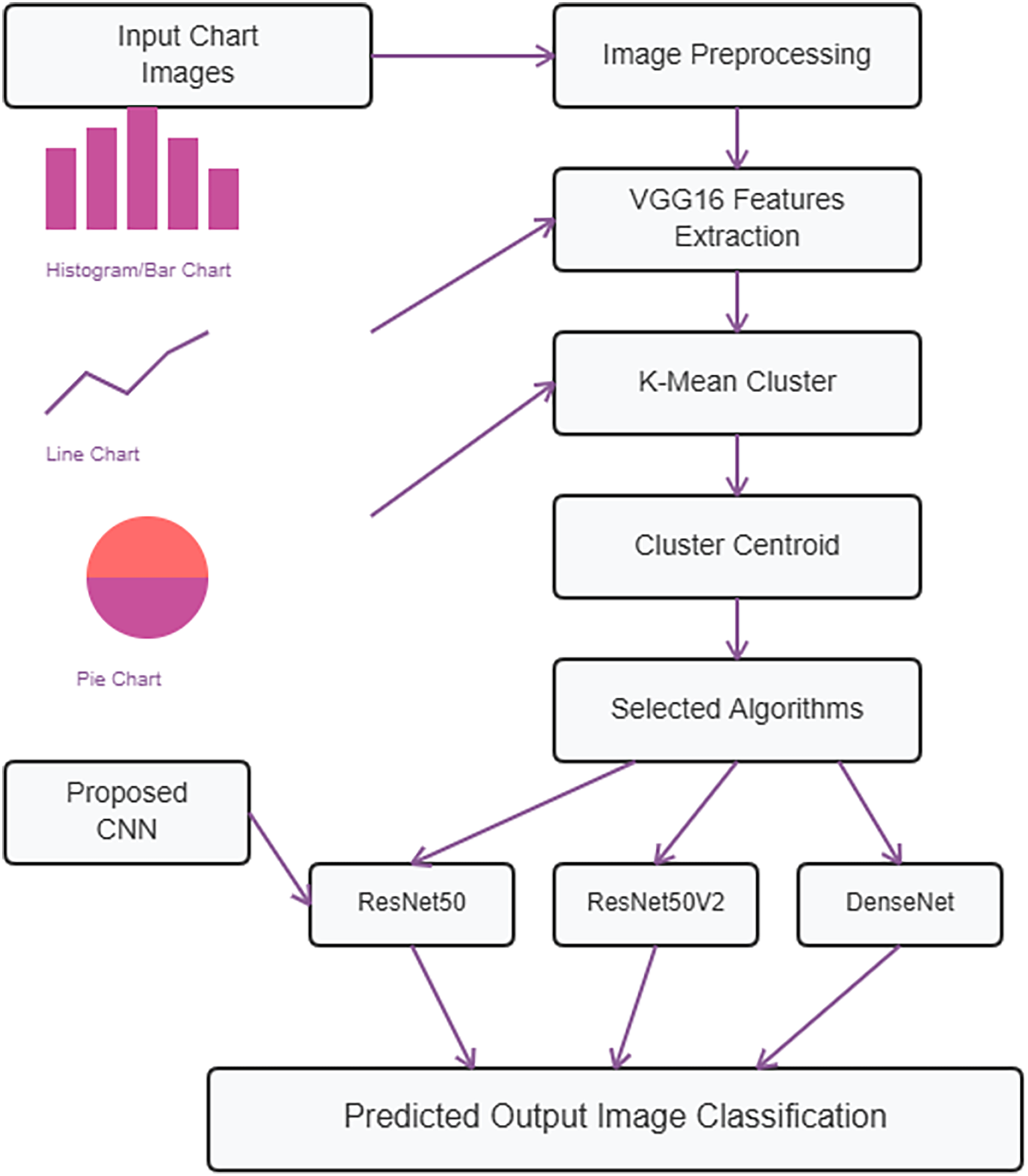
Figure 1 illustrates the process where chart images are provided as input and subjected to preprocessing techniques. Following this, feature vectors are computed using VGG16. Subsequently, K-means clustering is employed to identify clusters. Finally, a customized CNN along with ResNet50, ResNet50V2, and DenseNet are utilized for image classification, producing the final output.
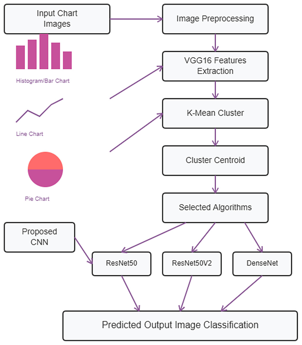
Figure 1: Proposed methodology diagram.
About dataset
In this study ChartVQA dataset was selected due to its diverse large-scale and realistic data from real-world articles and reports charts images for visual question answering (VQA) tasks. Datset consists of 20,882 chart images with four major chart types such as 2,882 histogram, 4,000 pie, 8,000 bar images and 6,000 line chart images. Multi-class chart classification tasks are well-suited for it.
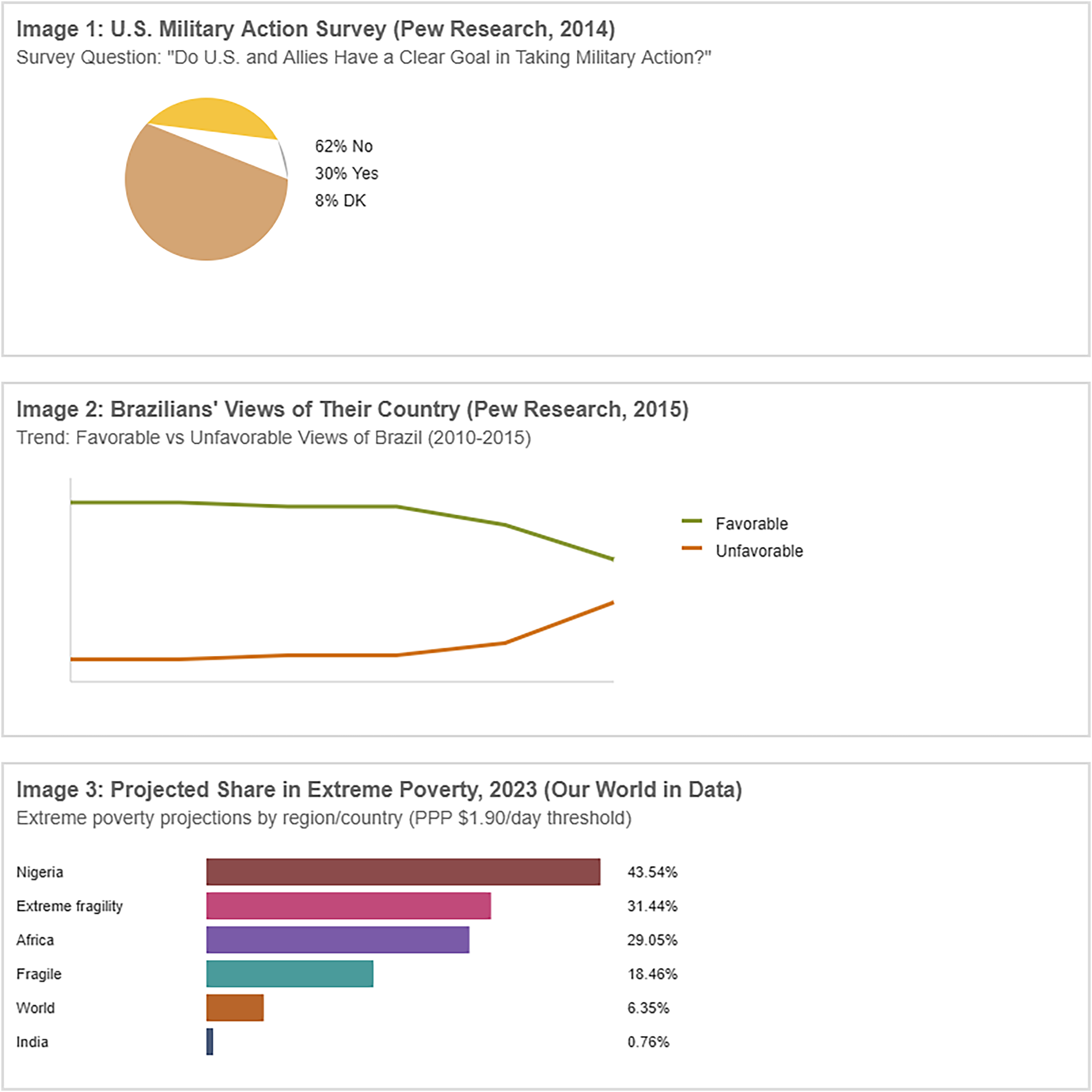
Figure 2 contains some sample images from a dataset that is used for training our model. The actual dimensions of images are 224 × 224 pixels which are reduced during preprocessing step.

Figure 2: Sample of training images from dataset.
Data preprocessing
The original chart images in PNG format are resized to 200 × 200 pixels in RGB format to maintain consistency across the dataset. This resizing is essential for ensuring compatibility with the VGG16 model used for feature extraction. Additionally, the pixel values are scaled to the range [0, 1] by dividing each value by 255. Stabilizing the training process through normalization during preprocessing is crucial, as it prevents gradients from becoming too large or too small during backpropagation. Figure 3 shows the sample resize image of bar chart, similarly all images are resized.
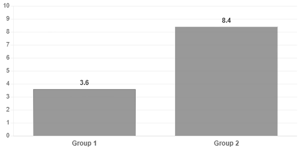
Figure 3: Sample size.
Features extraction and clustering
The pretrained VGG16 model is used for feature extraction from the block5_pool layer, offering both computational efficiency and strong performance, particularly in unsupervised learning scenarios. It is more interpretable and easier to manage when extracting visual features such as edges, textures, and spatial patterns from the final convolutional block, due to its use of 3 × 3 convolutional layers and 2 × 2 max-pooling layers compared to more complex architectures like Xception, EfficientNet, or Inception.
Clustering with K-means and PCA
Extracted features from VGG16 from the block5_pool layer of VGG16 were first reduced using PCA. Approximately 200–300 dimensions were reduced and retained the top components that explained 95% of the total variance which helpful for K-means algorithm by removing noise and redundant features. K = 4 clusters was chosen due to match with chart types in dataset to validate visual separability among these four types. An unsupervised pipeline that was streamlined and interpretable without excessive computational overhead was made possible by the combination of VGG16, PCA, and K-means.
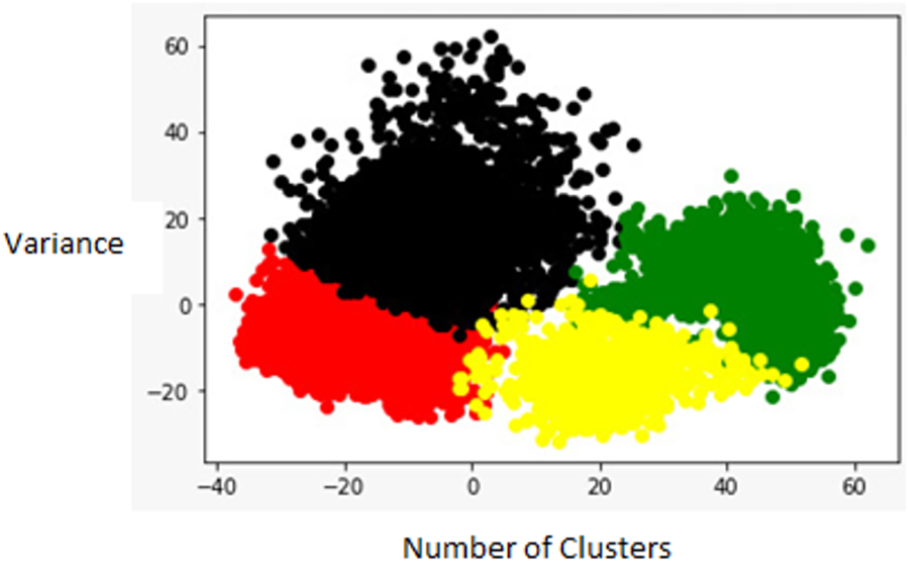
Figure 4 shows the actual data points of images computed by VGG16 for and Fig. 5 is four group cluster generated by k-means.
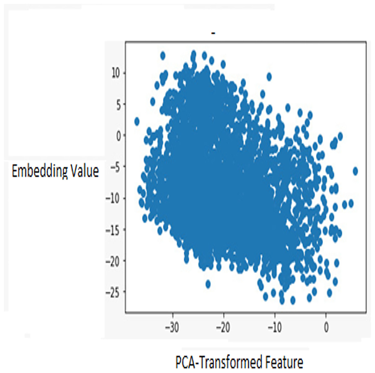
Figure 4: Featured DataPoint.
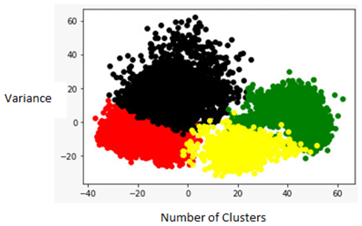
Figure 5: KMean_Cluster.
Selected algorithms
CNN architecture is used for the image classification task due to its ability to autonomously learn hierarchical features from data. All selected models are designed to capture both low-level and high-level attributes from input images for accurate classification into chart types (histogram, bar chart, line chart, pie chart). The proposed custom CNN model uses 32 filters of size 3 × 3 and includes a max-pooling layer to classify chart images. Additionally, models such as ResNet50 and ResNet50V2, both pretrained on ImageNet, are employed to learn complex patterns in chart images through their deep residual learning capabilities. Finally, DenseNet improves classification efficiency by enabling feature reuse and reducing the number of parameters. The parameters used to train and validate the models are summarized in Table 2.
| Model | Input size | Conv layer | Activation function | Pooling layer | Dropout rate | Output layer | Learning rate | Epochs | Batch size | Optimizer | Loss function |
|---|---|---|---|---|---|---|---|---|---|---|---|
| Custom CNN | 224 × 224 × 3 | 32 filters, 3 × 3 kernel | ReLU (Dense), SoftMax | Max Pooling (2 × 2) | 0.25 | SoftMax | 0.001 | 30 | 32 | RMSProp | Categorical Crossentropy |
| ResNet50 | 200 × 200 × 3 | Pre-trained on ImageNet | ReLU, SoftMax | – | 0.5 | SoftMax | 0.001 | 30 | 32 | RMSProp | Categorical Crossentropy |
| ResNet50V2 | 200 × 200 × 3 | Pre-trained on ImageNet | ReLU, SoftMax | – | 0.5 | SoftMax | 0.001 | 30 | 32 | RMSProp | Categorical Crossentropy |
| DenseNet | 200 × 200 × 3 | Pre-trained on ImageNet | ReLU, SoftMax | – | 0.5 | SoftMax | 0.001 | 30 | 32 | RMSProp | Categorical Crossentropy |
Implementation details
Hardware
All experiments were conducted using Google Colab Pro, which provided the following computational resources:
GPU: NVIDIA Tesla T4
CPU: Single-core Intel Xeon
RAM: 13 GB
Software
The implementation environment was based on:
Operating system: Ubuntu-based Colab virtual environment
Programming language: Python 3.9
Deep learning libraries: TensorFlow 2.12, Keras
Supporting libraries: NumPy, Matplotlib, Scikit-learn
Results and discussion
To ensure reliable model evaluation and prevent overfitting, the dataset was divided into 60% training, 20% validation, and 20% test sets. This 60/20/20 split is widely accepted in machine learning practice, especially when the dataset size is moderately large as is the case with our dataset of 20,882 chart images. The 60% training set provides sufficient data for learning, the 20% validation set allows for hyperparameter tuning and early stopping decisions, and the 20% test set enables robust evaluation of model generalization. To maintain class balance across all split’s, stratified sampling was applied during data partitioning. This ensured that each of the four classes (bar chart, line chart, pie chart, histogram) retained approximately the same proportion in the training, validation, and test sets as in the original dataset. The original dataset has a natural imbalance (e.g., bar charts = 8,000, histograms = 2,882), so preserving these proportions during splitting was essential to avoid training bias or skewed performance evaluation.
Models training and validation accuracies and losses
All selected models, custom CNN, RestNet50, RestNet50V2 and DenseNet performance are measured with training and validation accuracies and losses. In this scenario, training is conducted over 30 epochs, meaning all models will go through the entire training dataset 30 times.
Model training CNN custom layer
Model training in CNNs involves optimizing the model’s boundaries to minimize a defined misfortune function while maximizing performance measurements. Figure 6 shows training and validation accuracy and loss over multiple 25–30 epochs. Training accuracy increases steadily and reaches a high level, surpassing 0.9825 (98.25%) by the final epochs. This consistent rise suggests that the model effectively learn patterns in the training data and fit it well. The validation accuracy starts around 0.0198 and fluctuates over the different epochs and reaches significant upward trend then finally it stabilizes around 0.90–0.92. On the other hand, at initial epochs (Epochs 0–3), both training and validation loss decrease initially, indicating that the model is learning and reducing errors on both the training and validation sets. The decrease in training loss is sharper than that in validation loss, which is typical as the model starts to fit the training data. The training loss continues to decrease steadily, indicating ongoing improvement in fitting the training data. However, validation loss fluctuates, showing noticeable peaks around different epochs. These fluctuations suggest that the model is experiencing some challenges in generalizing to the validation set, potentially due to slight overfitting or an unoptimized learning rate.
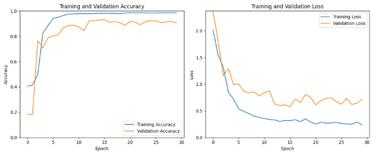
Figure 6: Custom CNN train and valid loss and accuracy.
Model training ResNet50 V1
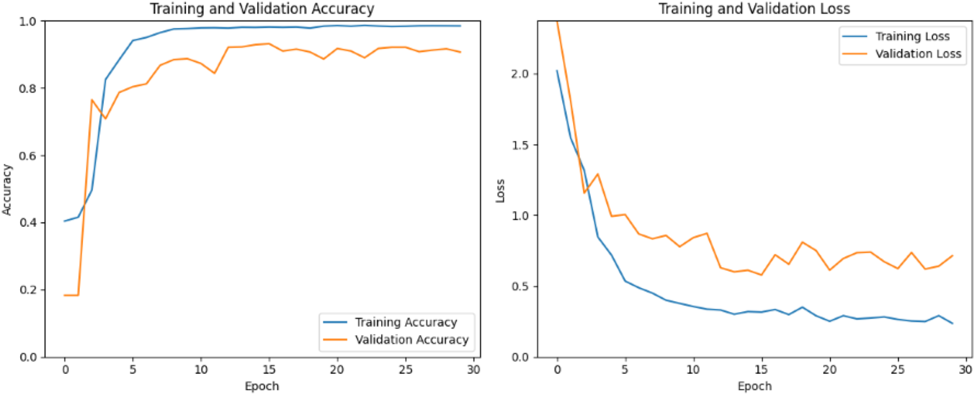
By selecting ResNet50, the top layers of the pretrained model, commonly comprising dense layers responsible for classification, are disposed of, retaining the convolutional base. This stage involves iteratively adjusting the model’s boundaries to minimize a defined misfortune function while maximizing performance measurements. In Fig. 7, the training and validation accuracy graphs start at around 80% of the initial epochs. The accuracy continues to increase during training but experiences a dip between the 12th and 15th epoch before rising again to nearly 85%. The validation accuracy curve exhibits some fluctuations but eventually converges with the training accuracy in the final epochs. However, the training and validation loss graphs reveal a significant amount of validation loss, indicating that the current model is not adequately trained under the same parameters provided to other models. This suggests that the model may require further tuning or adjustments to improve its performance and reduce the validation loss.
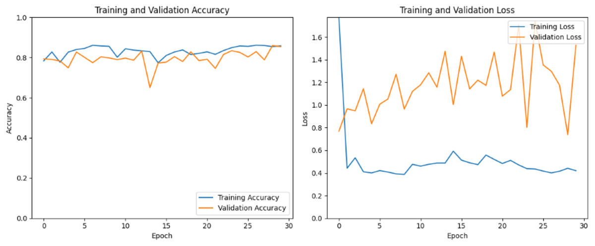
Figure 7: ResNetV1 train and valid loss and accuracy.
Model training ResNet50 V2
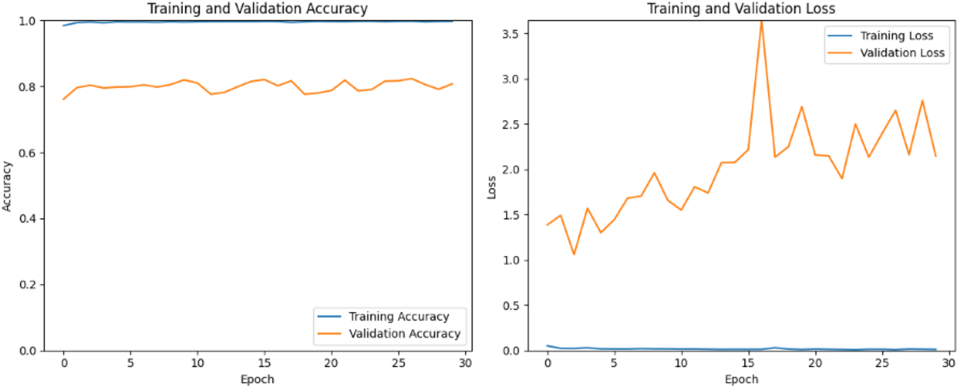
ResNet50 v2 incorporates several enhancements, such as batch normalization after each convolution and the use of identity mappings, which help in mitigating the vanishing gradient problem and improving gradient flow. In Fig. 8 the training accuracy remains nearly constant at a high value (close to 1.0), indicating the model is performing extremely well on the training dataset. The validation accuracy fluctuates and remains significantly lower than the training accuracy, with no clear upward trend. The large gap between training and validation accuracy suggests the model is overfitting to the training data. The lack of improvement in validation accuracy indicates the model struggles to generalize to unseen data, possibly due to insufficient regularization or a lack of diverse features in the training set. The training loss is consistently very low, which aligns with the high training accuracy. Validation loss is much higher and fluctuates significantly, with a notable spike around epoch 15 and continued instability thereafter. The divergence between training and validation loss further confirms overfitting. The spike in validation loss could indicate instability during training, possibly caused by a learning rate that is too high or by overfitting to the training data. The model fits the training data almost perfectly but fails to generalize with the validation data.
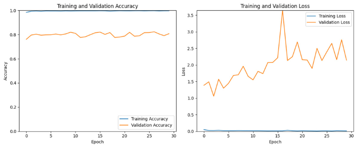
Figure 8: ResNetV2 training and validation loss and accuracy.
Model training DenseNet
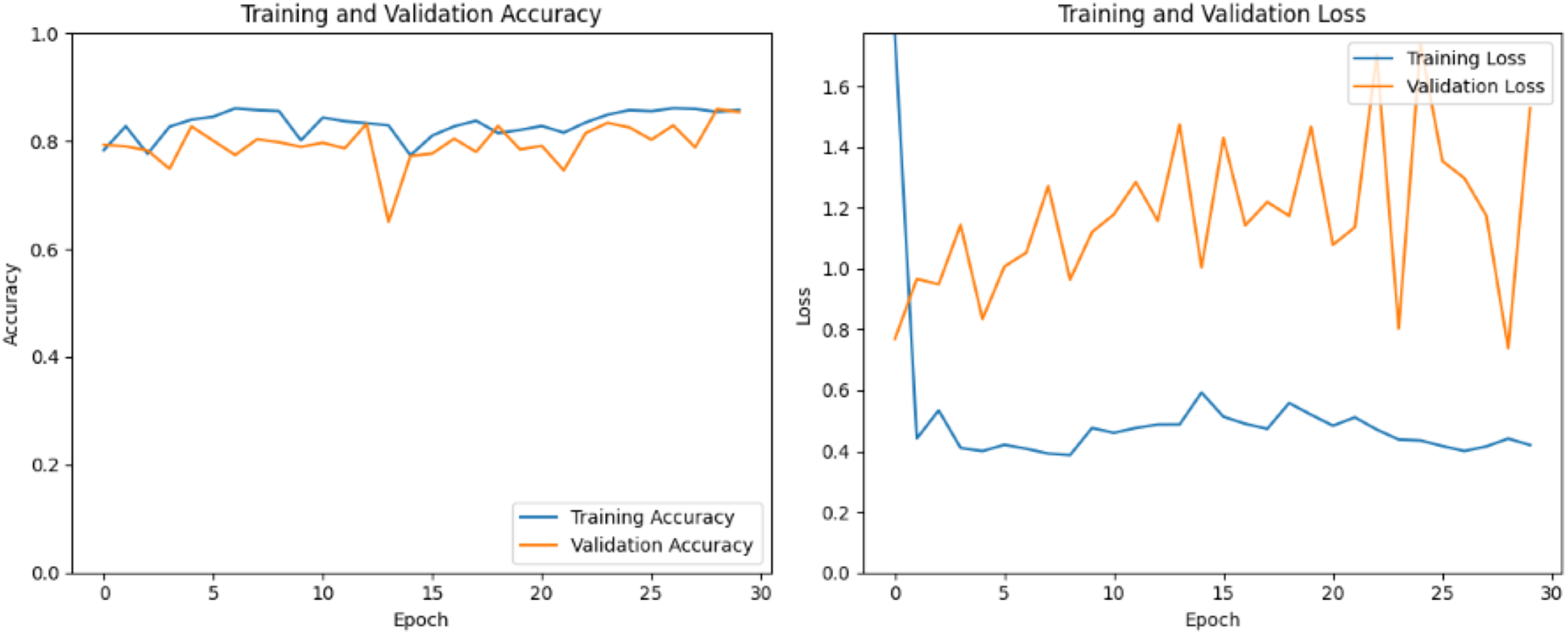
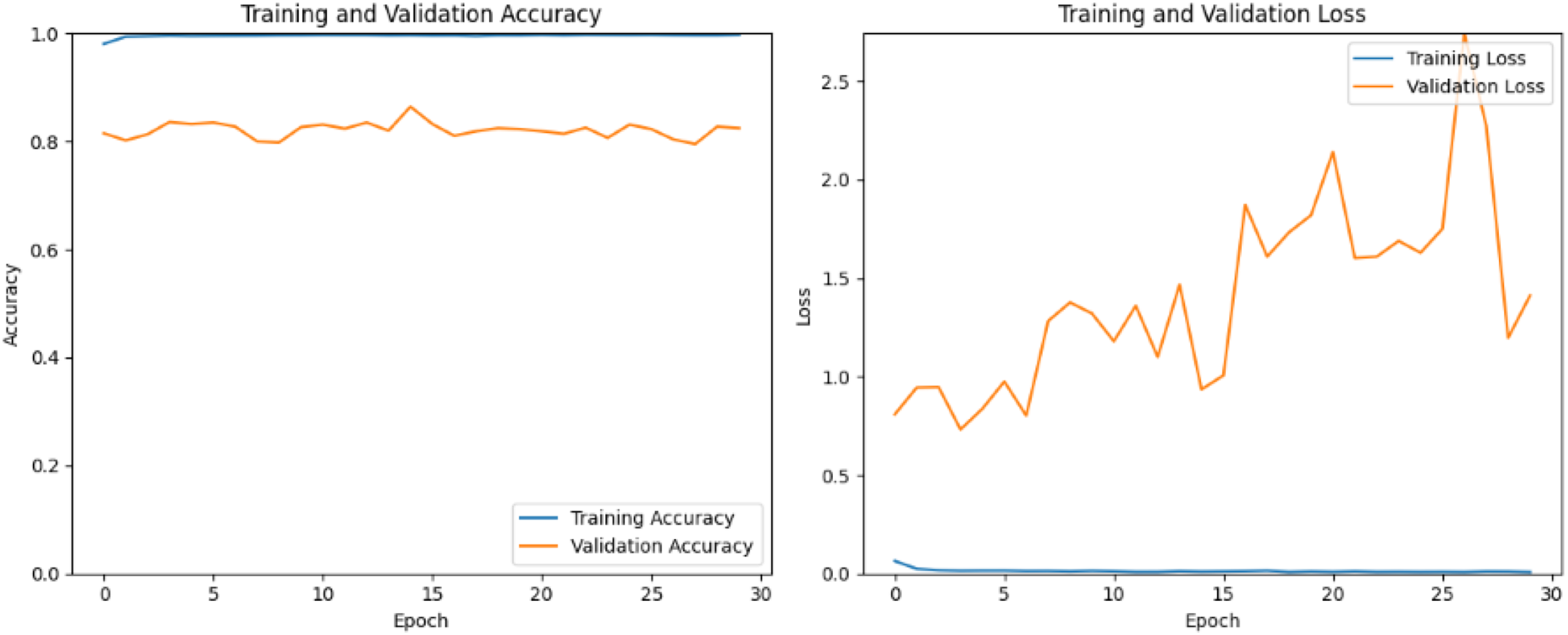
DenseNet, short for dense convolutional network, is chosen for its unique architecture described by dense connectivity patterns between layers. Unlike traditional CNNs where each layer is connected only to the subsequent layer, DenseNet lays out direct connections between all layers within a dense block. Figure 9 shows the training process has yielded a perfect training accuracy of 100%, however, the validation accuracy stands at approximately 80%. This discrepancy suggests that while the model has learned to classify the training data flawlessly, it may be overfitting, meaning it has memorized the training data rather than learning to generalize from it. The 80% validation accuracy indicates that the model’s performance drops when applied to new, unseen data. The training process has shown a consistent training loss of nearly 0% across all 30 epochs, indicating that the model has effectively learned the training data. However, the validation loss presents a different story, initially increasing steadily from 0.8 to 3 over various epochs, suggesting that the model was struggling to generalize to unseen data and was likely overfitting. Interestingly, from epoch 25 to 30, the validation loss began to decrease, reaching 1.3 by the 30th epoch.
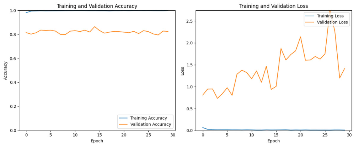
Figure 9: DenseNet train and valid loss and accuracy.
Models confusion matrix
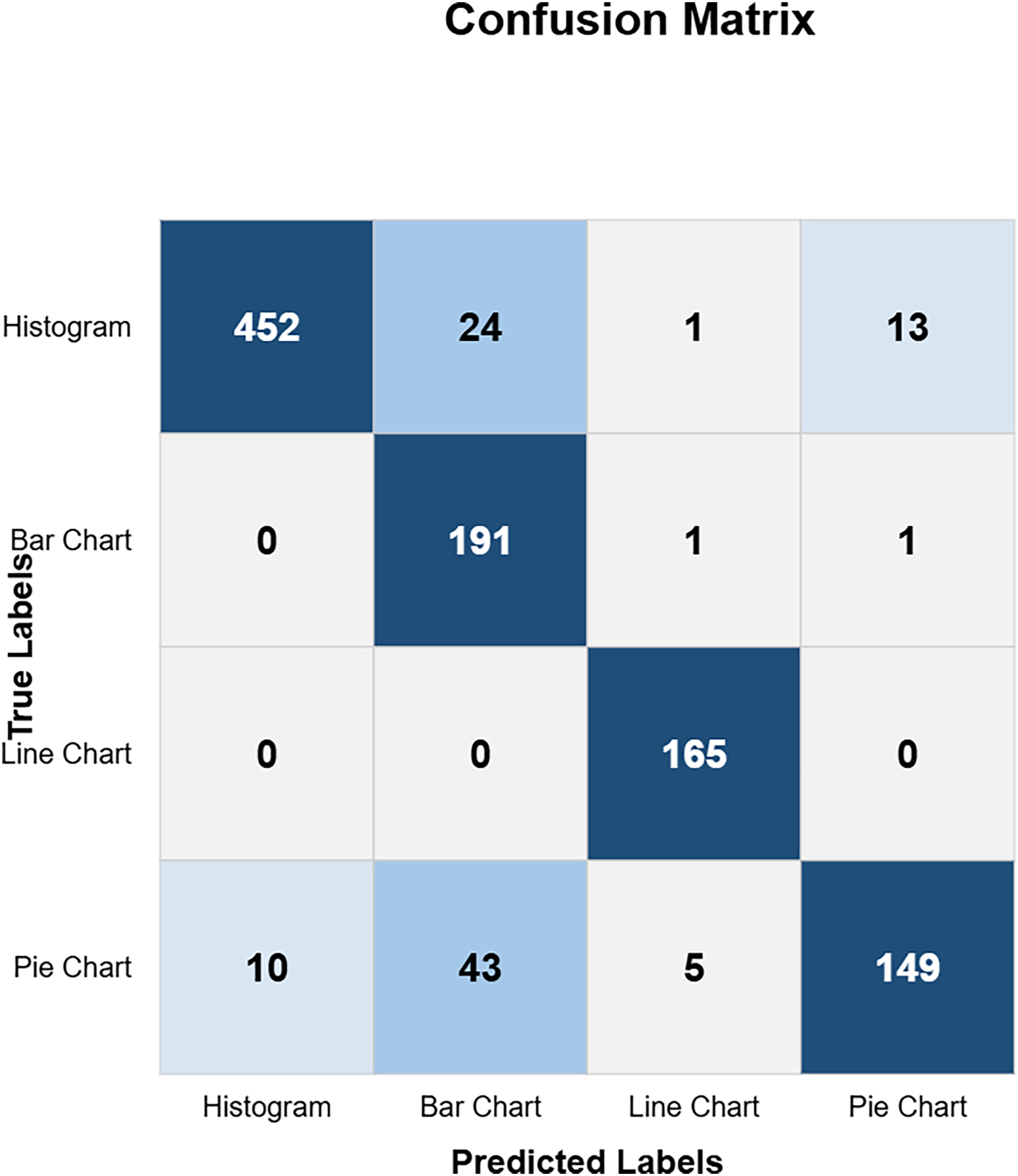
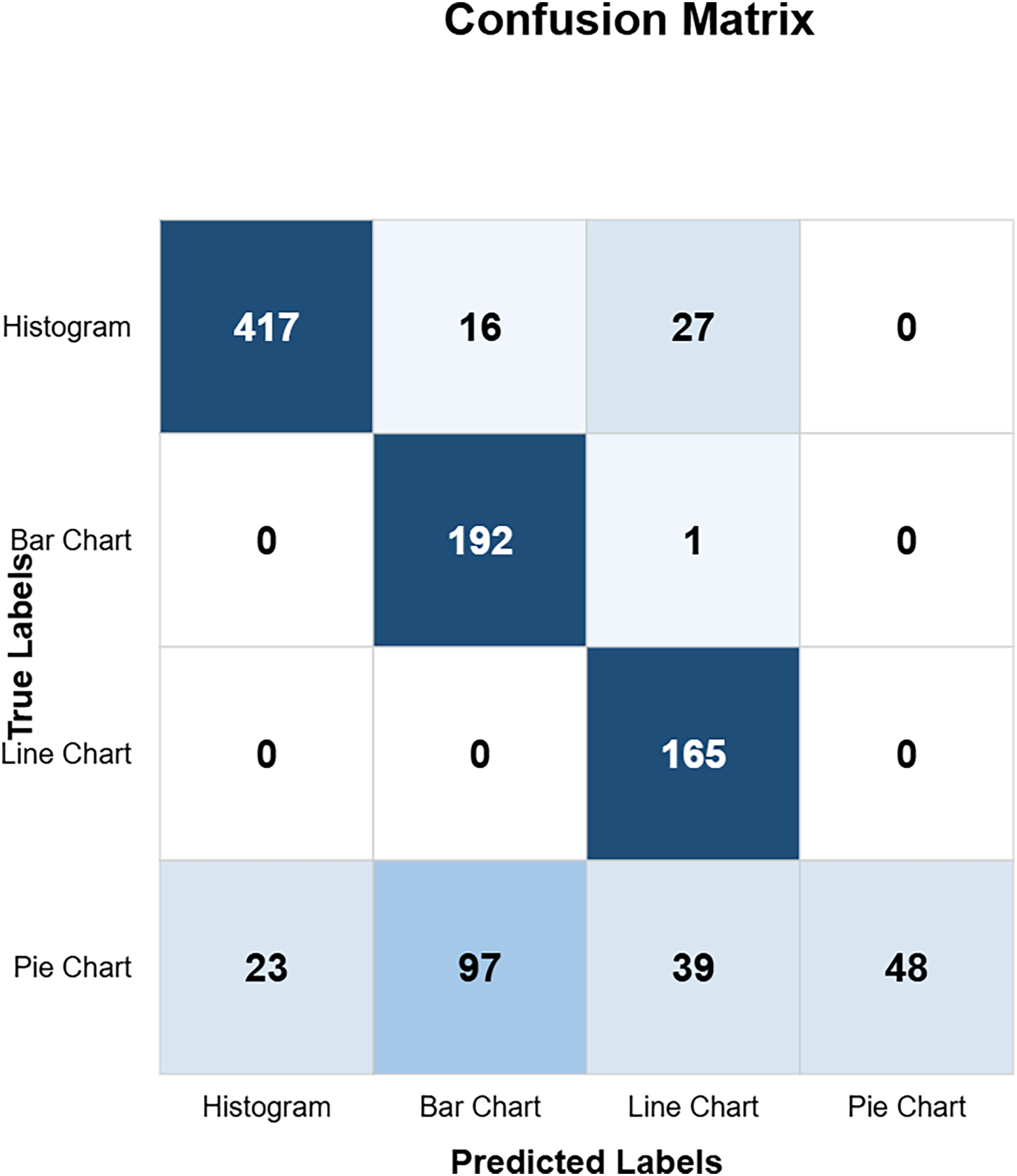
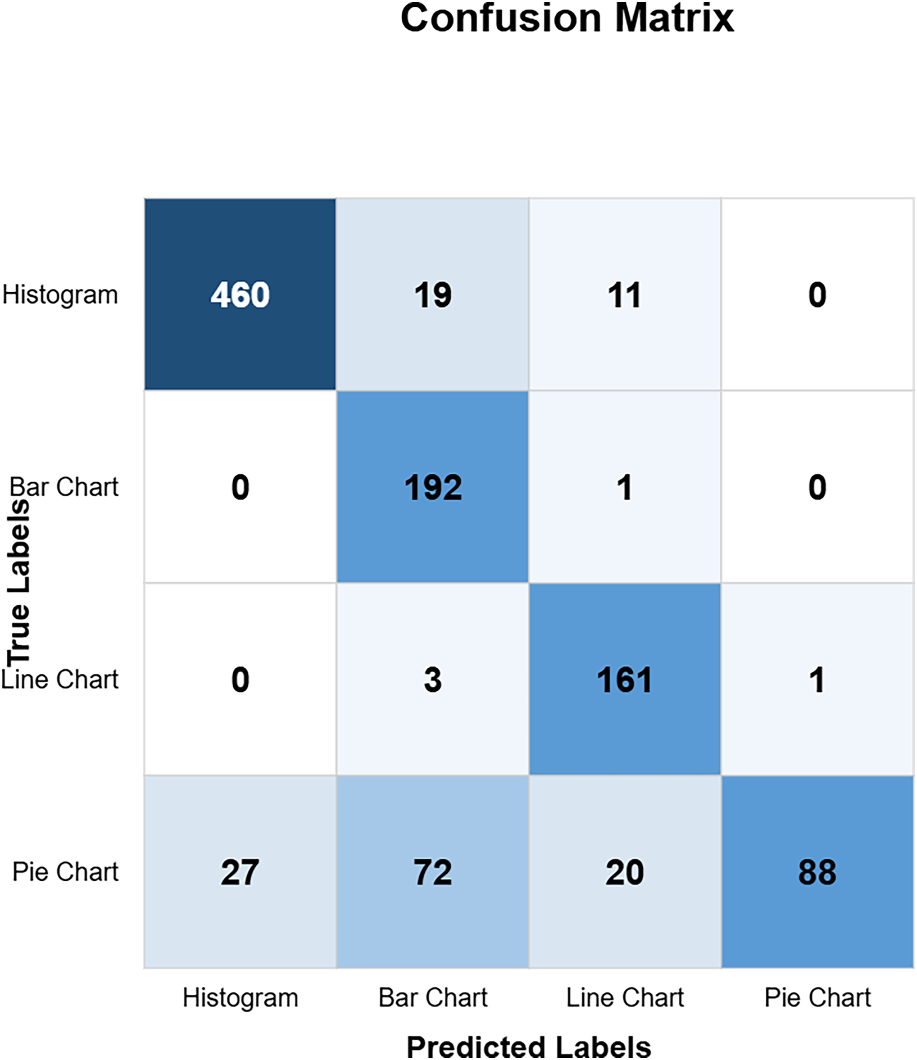
The confusion matrix in Fig. 10 shows the custom CNN model’s high classification accuracy with 452 histograms, 191 bar charts, 165 line charts, and 149 pie charts as true positives, indicating its robustness and effectiveness. The model produced very few misclassified values, indicating that it performs exceptionally well overall. This high level of accuracy across different chart types demonstrates the model’s robustness and effectiveness in correctly identifying various visual data representations. Figure 11 highlights the model ResNet50V1 high accuracy for histograms (460), bar charts (192), and line charts (161), but it struggles with pie charts correctly identifying only 88 and frequently misclassifying other charts as pie charts. This indicates a notable weakness in the model’s ability to accurately distinguish pie charts from other types of visual data representations. In Fig. 12, the ResNet50V2 model shows high accuracy for histograms (447) with few misclassifications (16 bar charts, 27 line charts, 0 pie charts), but it struggles with pie charts, correctly identifying only 48 and often misclassifying other charts as pie charts. The confusion matrix for the DenseNet model in Fig. 13 shows it correctly identified 12 histograms but misclassified 467 as bar charts, failed to correctly predict any bar charts, misclassifying 192 as histograms, performed well for line charts (165 correct), but struggled with pie charts, correctly identifying only 55 and misclassifying many as other types.

Figure 10: Custom CNN confusion matrix (CM).
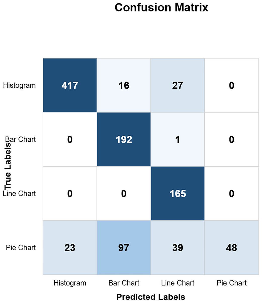
Figure 11: RestNetV1 confusion matrix (CM).
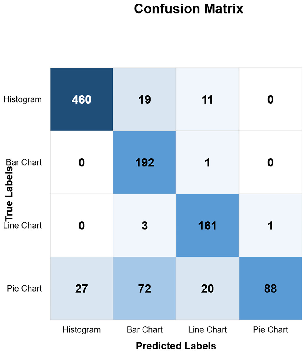
Figure 12: ResNetV2 confusion matrix (CM).
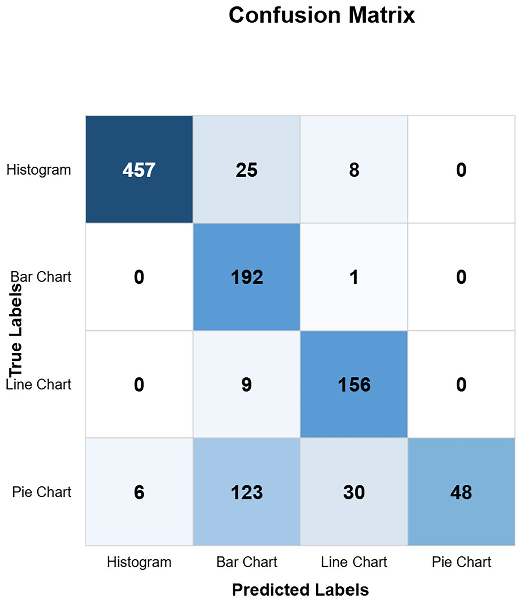
Figure 13: DensNet confusion matrix (CM).
Standard evaluation metrics, including accuracy, precision, recall, F1-score, and area under the curve (AUC), were computed to assess the performance of all models. Table 3 presents the highest accuracy (90.71%) and AUC (0.94) achieved by custom CNN, indicating its strong ability to balance sensitivity across all chart classes. ResNet50 achieved an accuracy of 85.40%, suggesting a tendency to miss certain chart types. Other models, such as ResNet50V2 and DenseNet, showed overall lower performance, particularly struggling with the identification of pie charts. These findings are consistent with the confusion matrix analysis (Figs. 10–13), where the custom CNN architecture effectively classified images compared to the other models, which frequently misclassified charts due to their complex internal representations.
| Model | Accuracy (%) | Precision (%) | Recall (%) | F1-score (%) | AUC (macro) |
|---|---|---|---|---|---|
| Custom CNN | 90.71 | 91.2 | 90.1 | 90.6 | 0.94 |
| ResNet50 | 85.40 | 86.3 | 83.5 | 84.8 | 0.89 |
| ResNet50V2 | 80.76 | 81.0 | 79.2 | 80.1 | 0.86 |
| DenseNet | 82.46 | 84.5 | 78.4 | 81.3 | 0.87 |
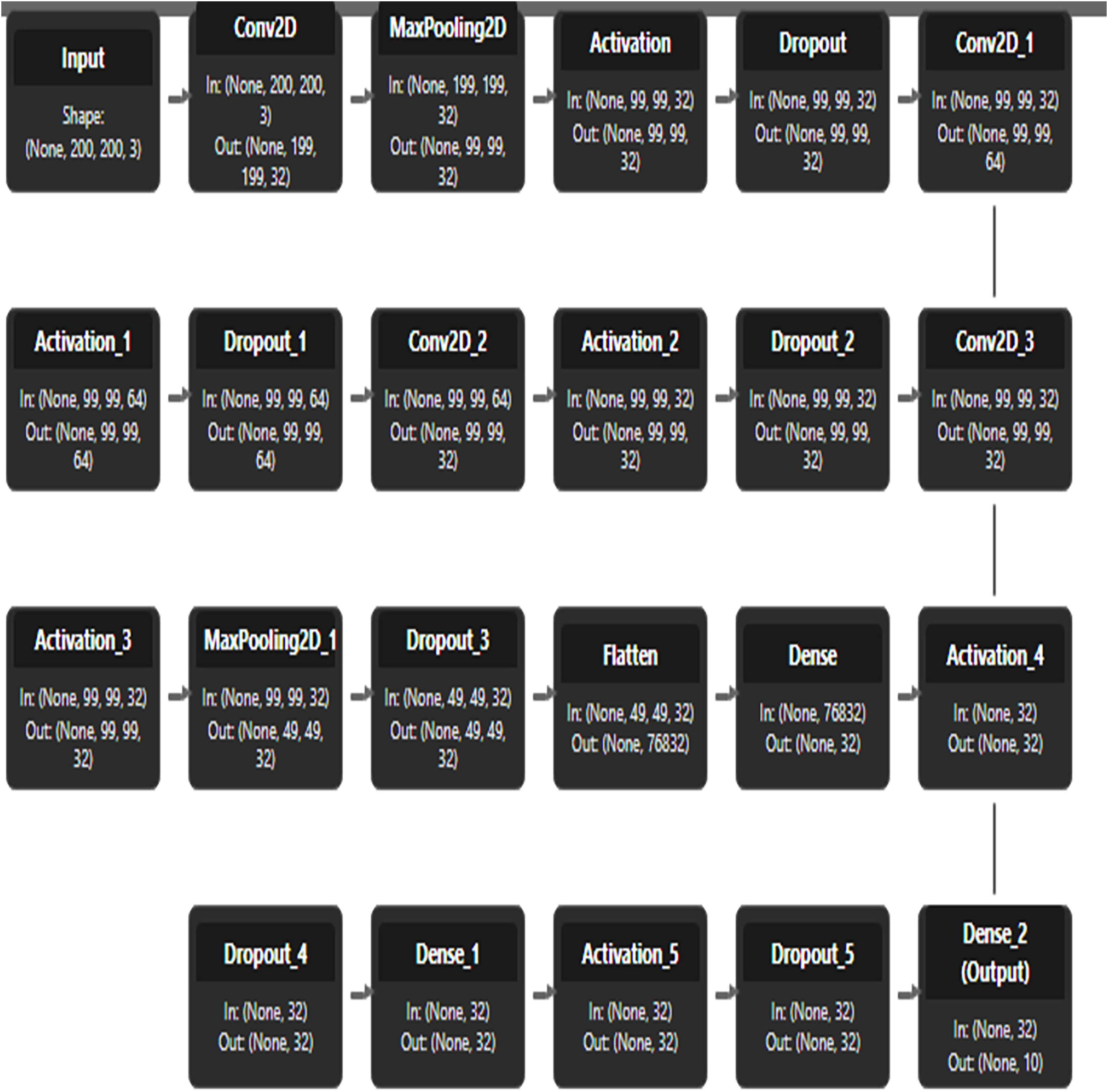
Figure 14 illustrates the custom CNN architecture, starting with an input size of 200 × 200 × 3. The input is processed through an initial convolutional layer (Conv2D) with 32 filters, followed by three sequential convolutional blocks to extract hierarchical features. The output is then passed through two dense layers with 32 units each, leading to the classification head where 2D feature representations are finalized. Complete architecture showcases a systematic approach to image classification through progressive feature abstraction and dimensionality reduction.
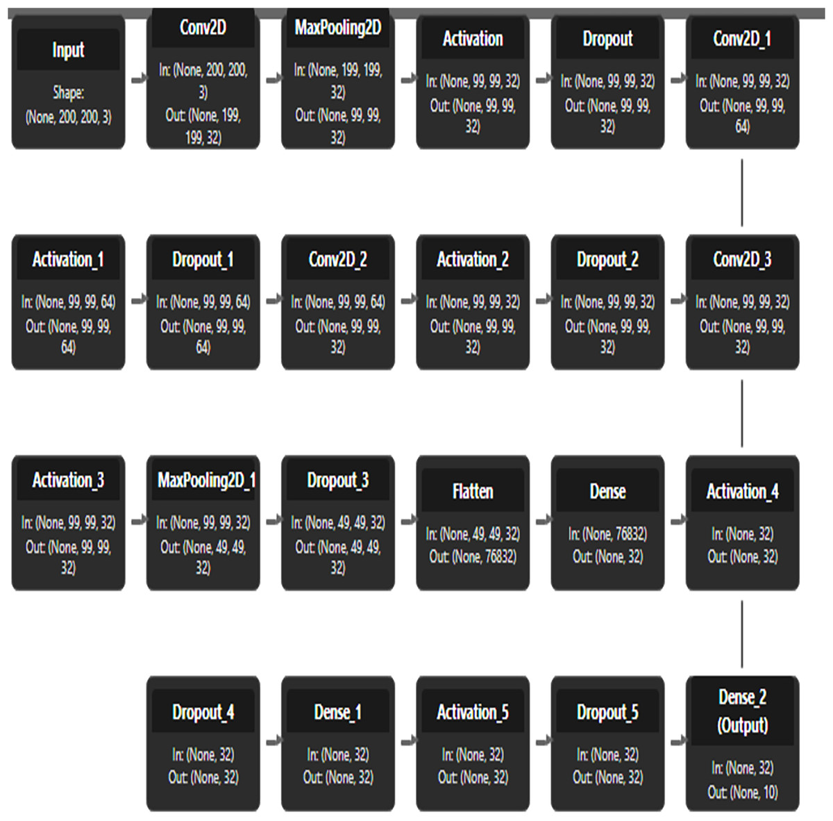
Figure 14: CNN architecture.
Model performance
Among all evaluated models, our proposed custom CNN architecture consistently achieved the highest overall accuracy, demonstrating strong generalization across all four chart types. In contrast, DenseNet, while powerful in general-purpose vision tasks, showed the lowest performance, particularly on pie charts. DenseNet often misclassified pie charts as bar or donut charts, likely due to its sensitivity to overlapping visual features and complex internal representations that are not well-suited to the stylistic variability in pie charts. On the other hand, custom CNN designed with domain-specific simplicity effectively captured geometric and structural distinctions (e.g., segment shapes, axis lines) with fewer parameters and lower risk of overfitting. This contrast highlights the advantage of lightweight, task-specific architectures for structured visual data like chart images.
Table 4 presents a comparative analysis of the execution times for four deep learning models used in the chart image classification task. The custom CNN model demonstrates the fastest overall training and validation time, completing 30 epochs in approximately 5 min due to its lightweight architecture and fewer parameters. In contrast, the pretrained models ResNet50, ResNet50V2, and DenseNet exhibit longer training and validation times, ranging from approximately 13 to 17 min in total.
| Model | Training time (30 epochs) | Validation time (Per epoch) | Total execution time | Notes |
|---|---|---|---|---|
| Custom CNN | 4 min 30 s | 8 s | ~5 min | Lightweight model with fewer parameters |
| ResNet50 (Pretrained) | 12 min 10 s | 10 s | ~13 min | Deeper architecture, slower convergence |
| ResNet50V2 (Pretrained) | 13 min 40 s | 12 s | ~15 min | Improved gradient flow, higher cost |
| DenseNet (Pretrained) | 15 min 30 s | 11 s | ~17 min | High feature reuse, heavier model |
Conclusions
In conclusion, this study on chart image classification using clustering techniques and deep feature extraction demonstrated strong and competitive results across multiple models. Initially, features are extracted from chart images using a pre-trained VGG16 model and grouped using K-means clustering in an unsupervised manner. These clusters are then used to guide training of supervised models, including ResNet50, ResNet50V2, DenseNet, and custom CNN. Among these, custom CNN outperformed the others, achieving a classification accuracy of 90.71%, compared to 85.40% (ResNet50), 82.46% (DenseNet), and 80.76% (ResNet50V2).
Custom CNN’s effectiveness is attributed to its lightweight architecture, appropriate regularization, and task-specific design, which allowed it to generalize better, especially for visually diverse and underrepresented chart types like pie charts. In contrast, deeper models such as DenseNet showed signs of overfitting and struggled particularly with curved and abstract visual structures. Despite these promising results, several limitations exist. The dataset used, while comprehensive, consists mostly of web-extracted or synthetic charts and may not fully represent real-world chart variability.
A limitation of this research is that the model is trained on only four fixed chart types with labels in a single language, and it does not address embedded text within the charts. These aspects can be explored and enhanced in future work.
Future direction
The proposed model can be further trained on larger and more diverse datasets, including additional chart types such as radar charts, area charts, and Gantt charts. It can also be evaluated using benchmark datasets like PlotQA, LEAF-QA, DocVQA, and FigureQA. Future enhancements may include handling low-resolution images, embedded annotations, and multilingual labels within charts. The Friedman aligned rank test or the Wilcoxon signed-rank test will be used for further performance evaluation.