
Long-term forecasting of solar and wind energy patterns using deep learning
- Published
- Accepted
- Received
- Academic Editor
- Giovanni Angiulli
- Subject Areas
- Artificial Intelligence, Data Mining and Machine Learning, Data Science, Neural Networks
- Keywords
- Time series prediction, Data decomposition, FEDformer, LSTM, Solar, Wind
- Copyright
- © 2025 Zihan et al.
- Licence
- This is an open access article distributed under the terms of the Creative Commons Attribution License, which permits unrestricted use, distribution, reproduction and adaptation in any medium and for any purpose provided that it is properly attributed. For attribution, the original author(s), title, publication source (PeerJ Computer Science) and either DOI or URL of the article must be cited.
- Cite this article
- 2025. Long-term forecasting of solar and wind energy patterns using deep learning. PeerJ Computer Science 11:e3114 https://doi.org/10.7717/peerj-cs.3114
Abstract
The significant volatility and randomness of renewable energy sources such as wind and photovoltaic power increase the operational uncertainty of power systems, while short-term forecasting struggles to capture monthly and seasonal characteristics of wind-solar data. To address the challenge of long-term time series prediction in renewable energy integration, this article proposes a wind-solar long-term time series prediction method based on a hybrid forecasting model combining Seasonal-Trend decomposition using Locally Estimated Scatterplot Smoothing (LOESS), Long Short-Term Memory, and Frequency Enhanced Decomposed Transformer. This approach combines the advantages of Frequency Enhanced Decomposed Transformer and Attention-Long Short-Term Memory Networks models, which have demonstrated excellent performance in time series prediction, and achieves complementary benefits through Seasonal and Trend Decomposition Using LOESS data decomposition. Experimental results show that the proposed method significantly improves Auckland wind sequence prediction, with mean squared error and mean absolute error reduced by up to 32.8% and 20.8% respectively, across different prediction horizons compared to existing classical prediction models.
Introduction
Driven by the “dual carbon” goals, China’s wind power and photovoltaic installation capacity has grown rapidly. As of 2024, wind and photovoltaic power generation capacity has exceeded 510 and 840 GW, respectively, accounting for over 13% and 20% of total capacity (Fekri, Ghosh & Grolinger, 2019). However, the random, intermittent and volatile characteristics of wind-solar resources pose significant challenges to power systems’ safe and stable operation. Therefore, accurately characterizing wind-solar uncertainty and generating high-precision time series has become a critical issue requiring urgent resolution.
Wind-solar time series generation methods mainly include probabilistic models, support vector machine (SVM), and deep learning approaches (Zhou et al., 2022). Probabilistic models fit historical data’s probability density functions through parametric or non-parametric estimation to generate random power output sequences. Li, Li & Wang (2021) models wind power prediction errors based on empirical T-distribution assumptions using parameter estimation methods. In Ma, Sun & Fang (2013) employs parameter estimation to identify solar irradiance distribution characteristics and constructs a photovoltaic power output distribution model considering irradiance effects. However, parameter estimation methods overly rely on prior knowledge of wind-solar probability distributions, and significant spatiotemporal differences exist in wind-solar characteristics across regions, making unified prior distributions prone to reduced model accuracy (Ma, Sun & Fang, 2013).
To overcome these limitations, references Fan et al. (2012), Chen et al. (2018) propose methods for identifying marginal distribution functions of wind-solar power output based on kernel density estimation, combined with Copula theory to construct joint probability distribution models. References Jiang et al. (2018), Fekri, Ghosh & Grolinger (2019) consider weather factor influences and propose correlation modeling methods based on vine Copulas. However, the modeling accuracy of non-parametric estimation methods heavily depends on the sufficiency of historical data, making it difficult to ensure reliable estimates when data is scarce. Moreover, probabilistic models primarily focus on long-term statistical characteristics of sequences and struggle to effectively characterize complex spatiotemporal correlations and other high-dimensional nonlinear features, limiting their application in long-term time series generation (Li, Li & Wang, 2021; Xie et al., 2017).
Given the superior nonlinear feature extraction and representation capabilities of deep learning methods, deep learning models represented by deep neural networks and generative adversarial networks (GANs) have gradually become research hotspots in wind-solar time series generation (Liang & Tang, 2020). In scenario generation research, GANs and variational autoencoders (VAEs), as two typical deep generative models, provide critical technical support for renewable energy scenario generation. These methods complement the innovative solutions proposed in this article, contributing to a more comprehensive understanding of scenario generation development.
In terms of GANs, Chen et al. (2018) pioneering work demonstrated GAN’s potential in renewable energy scenario generation and further proposed model-free data-driven methods suitable for different prediction ranges (Zhou et al., 2022). Subsequently, researchers made significant progress in improving GAN performance: enhancing model capability for handling mixed data through Bayesian methods (Ding, Bao & Bi, 2016), optimizing training convergence through improved network structures (Chen et al., 2018), and upgrading generation quality using Wasserstein distance (Chen, Wang & Zhang, 2018). Recent research has focused more on practical applications, such as Wang et al. (2025) unsupervised Conditional Generative Adversarial Network (CGAN) method (Chen, Li & Zhang, 2018) and temporal GAN model (Gu, Liu & Hu, 2021), providing effective approaches for solving practical engineering problems. In comparison, VAEs have shown unique advantages in scenario generation. Wang et al. (2018), pioneered the application of VAEs in wind-solar power generation scenario generation (Li, Li & Wang, 2021). At the same time, Huang et al. (2019) modular denoising VAE effectively improved the generation quality of multi-source-load scenarios (Ma et al., 2025). Notably, Wang et al. (2021)’s innovative approach combining VAE with graph neural networks (Liu et al., 2025) provided new insights for the precise modeling of complex scenarios. Although these studies have achieved significant progress in their respective fields, they share common limitations: model training requires large amounts of high-quality data, substantial computational overhead, and stability and reliability in handling complex scenarios still need improvement. These are precisely the key issues that our proposed innovative method aims to address. By leveraging the advantages of existing methods while overcoming their shortcomings, our solution achieves breakthroughs in computational efficiency and generation quality.
To address the aforementioned issues, this article proposes a time series prediction model based on STL-LSTM-FED, which integrates the advantages of Seasonal-Trend decomposition using LOESS (STL) data decomposition, Fedformer, and Attention-LSTM. The prediction accuracy is significantly improved by decomposing the original wind-solar time series data into periodic, trend, and residual components and separately training them using Attention-LSTM and Fed former.
Contributions
In this article, our contributions are as follows:
We developed a novel STL-LSTM-FED as a hybrid forecasting model combining Seasonal-Trend decomposition using Locally Estimated Scatterplot Smoothing (LOESS) (STL), Long Short-Term Memory (LSTM), and Frequency Enhanced Decomposed Transformer (FEDformer), for long-term wind-solar sequence forecasting. This model integrates STL, LSTM, and FEDformer to enhance prediction accuracy and reliability. By leveraging the strengths of each component, the model effectively captures both short-term fluctuations and long-term trends in wind-solar data. The integration of STL ensures the decomposition of complex time-series data into more manageable components, while the combination of LSTM and FEDformer enhances temporal feature extraction and sequence learning.
We also proposed a structured long-term wind-solar sequence prediction method that improves forecasting accuracy by decomposing time-series data into three key components: trend, seasonality, and residuals. The STL decomposition technique enables the separation of long-term trends from short-term fluctuations, thereby reducing noise in the data. The Attention-LSTM model is used for capturing periodic variations, while FEDformer effectively models long-term trends. This multi-step approach allows for a more precise and reliable prediction of wind-solar sequences.
We performed experiments by collecting real-world wind speed and solar radiation data from Auckland, New Zealand, covering the period from 2019 to 2023. From experimental study, the proposed STL-LSTM-FED model demonstrates significant improvements in renewable energy forecasting accuracy compared to existing models.
Rationale
The proposed STL-LSTM-FED methodology is designed to address key challenges in long-term forecasting of wind-solar time series, particularly the inherent randomness, intermittency, and spatiotemporal complexity of renewable energy sources. Traditional probabilistic and statistical models struggle with capturing nonlinear dependencies and require extensive prior knowledge of data distributions, while deep learning approaches such as GANs and VAEs demand large datasets and exhibit computational inefficiencies. To overcome these limitations, the proposed framework integrates STL, LSTM, and FEDformer to enhance both short-term fluctuation modeling and long-term trend prediction. STL decomposition allows for the separation of key time series components, reducing noise and improving feature extraction, while Attention-LSTM effectively captures periodic variations, and FEDformer enhances time series modeling using frequency-based attention mechanisms. The rest of the article is structured as follows. ‘Related Work’ describes the related work, ‘Proposed Framework’ discusses the proposed approach, ‘Experimental Setup and Results’ explains the experimental setup and results, and ‘Conclusions’ discusses the conclusions.
Related work
Zhu et al. (2023) proposed the SL-Transformer model for time-series wind and solar power forecasting. Wind power predictions were modelled, achieving a coefficient of determination (R2) of 0.9989 and a symmetric mean absolute percentage error (SMAPE) of 5.8507%. Solar energy forecasting achieved a SMAPE value of 4.2156%, indicating 15% improvement compared to competitor models. These findings highlight the strength of this model in specifying temporal dependencies in renewable energy data (Zhou et al., 2022). In 2023, Huang, Yan & Qu (2023) introduced a transformer-based model for predicting wind power. The attention mechanism used by the model enabled it to capture longer temporal dependencies in wind power data, leading to better accuracy in forecasting than conventional recurrent neural network-based models (Zhu et al., 2023). Tan et al. (2024) compared the Temporal Pattern Attention (TPA)-LSTM and Transformer model performance in predicting high-resolution electron fluxes at geostationary orbit (GEO). The Transformer model showed marginally improved performance, indicating its effectiveness in capturing complex temporal dependencies for space weather prediction tasks (Huang, Yan & Qu, 2023). Galindo Padilha et al. (2022) introduced a hybrid forecasting model combining transformer networks with traditional statistical methods for short-term renewable energy forecasting. The model effectively captured linear and nonlinear patterns in the data, enhancing prediction accuracy for wind and solar energy outputs (Tan et al., 2024). A hybrid forecasting model was devised by Ramesh & Arumugam (2024). They applied transformer networks to the traditional statistic relation methods to realize short-term renewable energy forecasting. Accurate predictions were driven for wind and solar outputs as data was evenly drawn from linear and non-linear patterns (Galindo Padilha et al., 2022). Zhang et al. (2023) used Transformer and Long Short-Term Memory (LSTM) algorithms to predict medium-term wind power production. The model was superior to an LSTM in capturing long-term dependencies and yielded more accurate predictions (Ramesh & Arumugam, 2024). Kumar, Paul & Vaidya (2020) performed a comparative study on different models important for steady-state solar wind forecasting (147). This study evaluated magnetic field extrapolation models alongside velocity empirical formulations to forecast solar wind parameters at the Lagrangian point L1 and provide insights into model performance and accuracy (Zhang et al., 2023). Jahin et al. (2024) reported a hybrid classical-quantum neural network called TriQXNet for forecasting the disturbance storm-time (Dst) index driven by solar wind. The model combined classical and quantum computing with conformal prediction and explainable artificial intelligence (AI), resulting in improved forecasting accuracy and the quantifiable uncertainty necessary for operational decisions (Kumar, Paul & Vaidya, 2020). Woolsey & Cranmer (2014) reported solar wind prediction models’ full magnetic field profile. Including the effects of Alfvén waves on coronal heating and wind acceleration, the results supported our contention that fast-mode wave heating is also present in solar wind conversions of kinetic energy. It emphasized the importance of incorporating detailed magnetic field geometry in forecasting models (Jahin et al., 2024). Bailey et al. (2021) improved ambient solar wind model predictions using a gradient-boosting regression method. Using data from a magnetic survey of the model, the machine learning approach came up with conditions at Earth that were better than the solar wind predictions of fungi24 or bpg G38. It also offers new vistas on what input material may mean in ambient solar wind modelling (Woolsey & Cranmer, 2014).
Table 1 describe some more literature reviews related to wind and energy forecasting.
| Reference | Approach used | Advantages | Limitations |
|---|---|---|---|
| Zhou et al. (2022) | FEDformer: Transformer-based model using frequency-enhanced decomposition for long-term time series forecasting. | Captures long-term dependencies; efficient for multivariate and long-sequence forecasting. | Limited interpretability; requires high computational resources. |
| Mahmoud & Mohammed (2021) | LSTM with attention mechanism for multivariate forecasting. | Good at modeling long temporal dependencies | Can struggle with long sequences; attention adds complexity. |
| Zhou et al. (2020) | Adversarial learning-based time series prediction using GANs. | Generates realistic synthetic data; handles nonlinearities well. | Training instability; lacks interpretability. |
| Kong et al. (2022) | Time-series GAN with an auxiliary classifier (ACGAN). | Improves generation quality by conditioning on labels. | Sensitive to mode collapse; requires careful tuning. |
| Sineglazov & Horbatiuk (2025) | Dual-Stage Attention-Based RNN for energy forecasting. | Combines input and temporal attention; good interpretability. | Complex architecture; overfitting risk with small datasets. |
| Lim & Zohren (2021) | Time-series Transformer for financial prediction. | Handles long-range dependencies; parallel training possible. | Requires large data for training; limited support for missing values. |
| Zerveas et al. (2021) | Transformer-based model with instance and channel mixing. | Effective for multivariate time series classification. | Not directly optimized for forecasting tasks. |
| Li et al. (2019) | Informer: Transformer model optimized for long sequence forecasting using sparse attention. | Efficient for long sequences; reduces computational cost via sparse attention. | Sparse attention may miss some critical temporal dependencies. |
| Wu et al. (2021) | Autoformer: Decomposition-based Transformer for long-term forecasting. | Models trend and seasonality explicitly; performs well on long horizons. | Limited interpretability; still computationally intensive. |
| Sen, Yu & Dhillon (2019) | DeepGLO: Global forecasting model for multivariate time series using graph neural networks. | Captures inter-series relationships; scalable to many time series. | Requires graph structure tuning; limited support for univariate series. |
| Salinas et al. (2020) | DeepAR: Probabilistic forecasting using autoregressive RNN. | Handles uncertainty and probabilistic outputs well. | Assumes strong autoregressive dependencies; struggles with abrupt shifts. |
| Hewamalage, Bergmeir & Bandara (2021) | Hybrid CNN-LSTM for time series forecasting. | Captures spatial and temporal features; suitable for structured data. | Complex architecture; higher training time. |
Proposed framework
We have applied STL decomposition to isolate the trend component, effectively removing dominant seasonal cycles. This isolation yields a detrended long-term component with reduced cyclic interference. At this stage, FEDformer’s multi-resolution frequency analysis becomes advantageous for detecting fine-grained, slowly varying structures within the trend component. Its Fourier Enhancement Block (FEB) is adept at identifying frequency-relevant trends even after annual periodicities are filtered out. Conversely, Attention-LSTM is assigned to model the periodic component, which still contains structured long-term cycles (e.g., seasonal, weekly, or daily variations). LSTM’s strength lies in sequential temporal learning, and the attention mechanism further amplifies its ability to retain long-span dependencies, making it well-suited for modeling these structured periodic features.
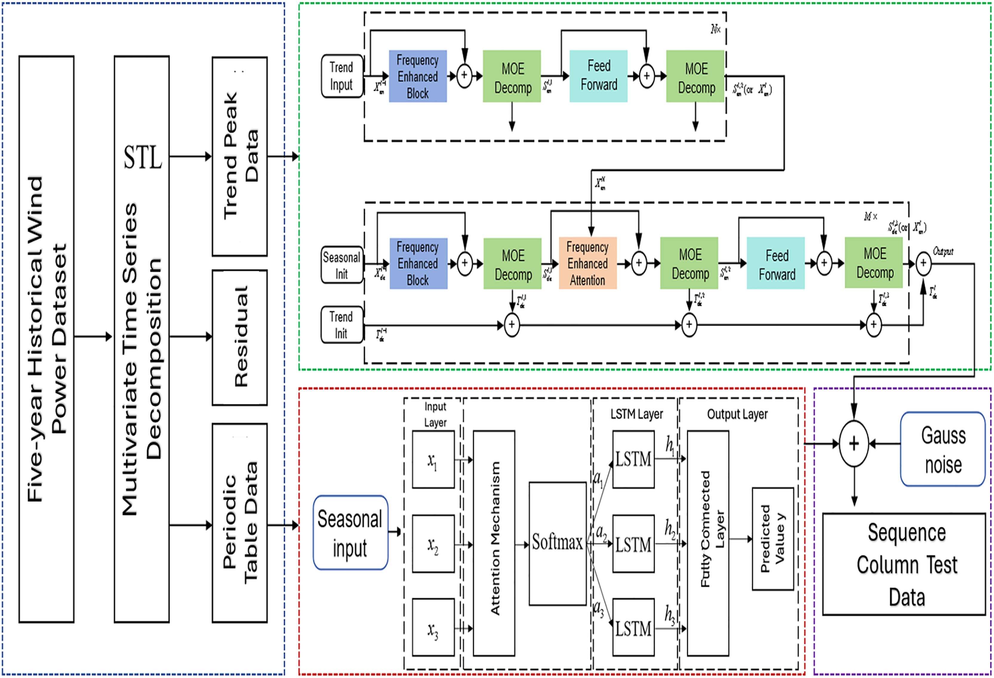
We have proposed a STL-LSTM-FED Model as shown in Fig. 1, with specific implementation steps as follows:
(1) Data Preprocessing: perform interpolation, anomaly removal, and standardization on the original wind-solar time series data.
(2) STL Sequence Decomposition: apply STL method to decompose standardized data into trend, periodic, and residual components. The decomposition period is set to 1 year to reduce seasonal interference with trend components.
(3) Trend Component Prediction: model trend components using the FEDformer model. This model is particularly suitable for processing short-period characteristic data and demonstrates strong predictive capability for trend components after annual cycle removal. During training, trend component data undergoes multi-level decomposition to extract finer-grained features.
(4) Periodic Component Prediction: process periodic component data using the Attention-LSTM model. This model excels in capturing long-period, slowly-varying features, effectively complementing FEDformer’s limitations in long-term scale modeling.
(5) Residual Component Generation: generate residual data conforming to statistical characteristics by fitting Gaussian distribution parameters based on temporal features of STL-decomposed residual components.
(6) Sequence Reconstruction: combine the trend, periodic, and residual component prediction results to obtain complete annual prediction sequences.
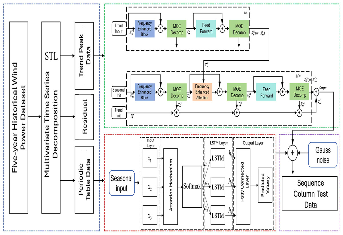
Figure 1: STL-LSTM-FED model structure.
This hierarchical prediction strategy effectively leverages the advantages of different models, significantly improving the prediction accuracy of long-term wind-solar sequences.
Long-term wind-solar sequence decomposition method
Characteristic analysis of wind-solar sequences
As typical multivariate time-series data, wind-solar time series possess fixed sampling frequencies and multidimensional features. Their main characteristics include:
Nonlinearity: sequences contain noise and abrupt changes.
Multimodality: sequences encompass multiple temporal patterns.
Scale differences: inconsistent dimensions exist between different sequences.
Correlation: multiple indicators exhibit coordinated evolutionary relationships.
Wind-solar time series forecasting can be categorized into short-term and long-term types based on prediction duration. Short-term prediction primarily applies to operational dispatching, reliability assessment, and fault tracking. In contrast, long-term prediction better captures renewable energy’s seasonality and continuity characteristics, playing crucial roles in power system planning and maintenance strategy formulation.
Seasonal characteristics of wind-solar sequences
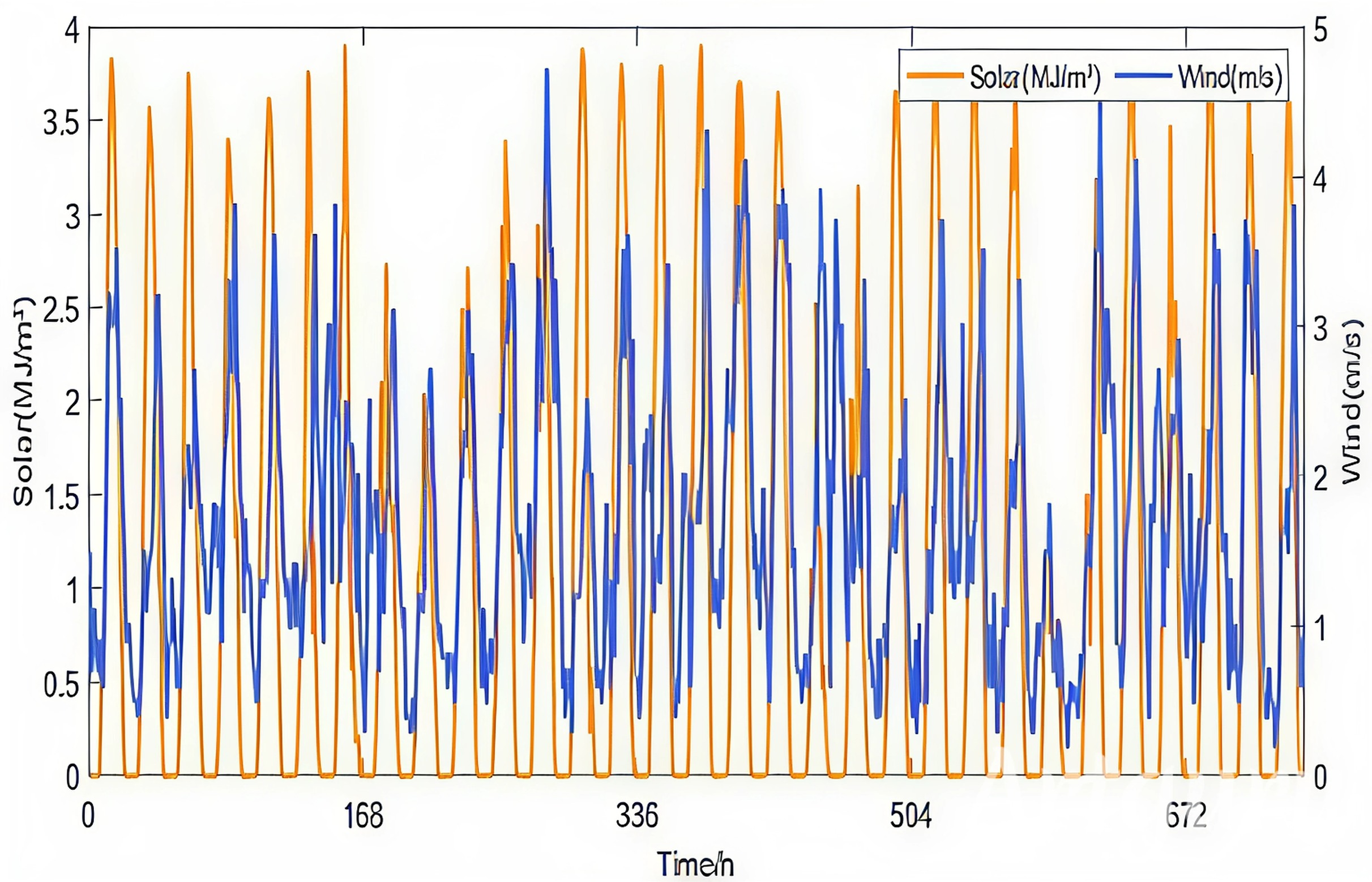
Renewable energy sources are directly influenced by climatic conditions, resulting in a significant correlation between wind speed and solar radiation. Existing research often treats wind speed and solar radiation scenario generation as independent processes. The prediction method proposed in this article fully considers the coupling relationship between wind and solar energy. As shown in Fig. 2, using wind speed and radiation intensity data from January 2022 exhibit clear synchronous fluctuation characteristics, with correlation coefficients shown in Table 2.
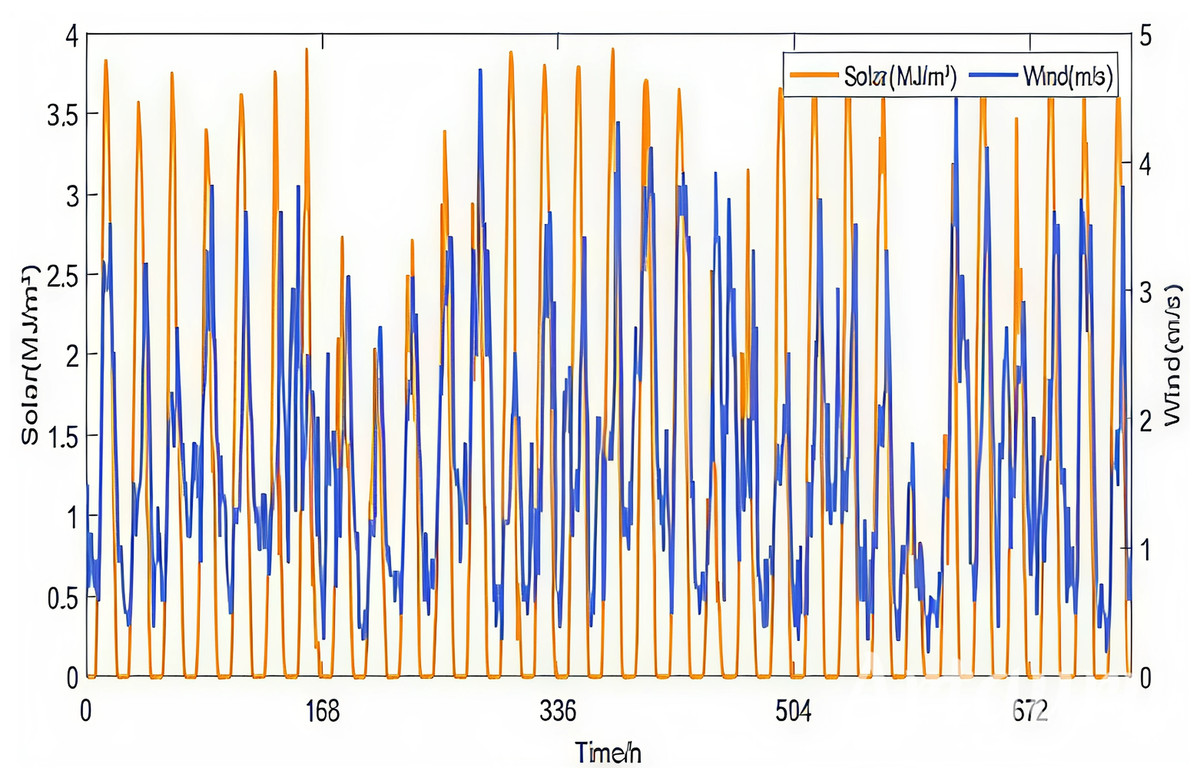
Figure 2: Change rule of wind speed-solar irradiation intensity in January 2022.
| Pearson | Spearman | Kendall | |
|---|---|---|---|
| r | 0.4804 | 0.3734 | 0.2663 |
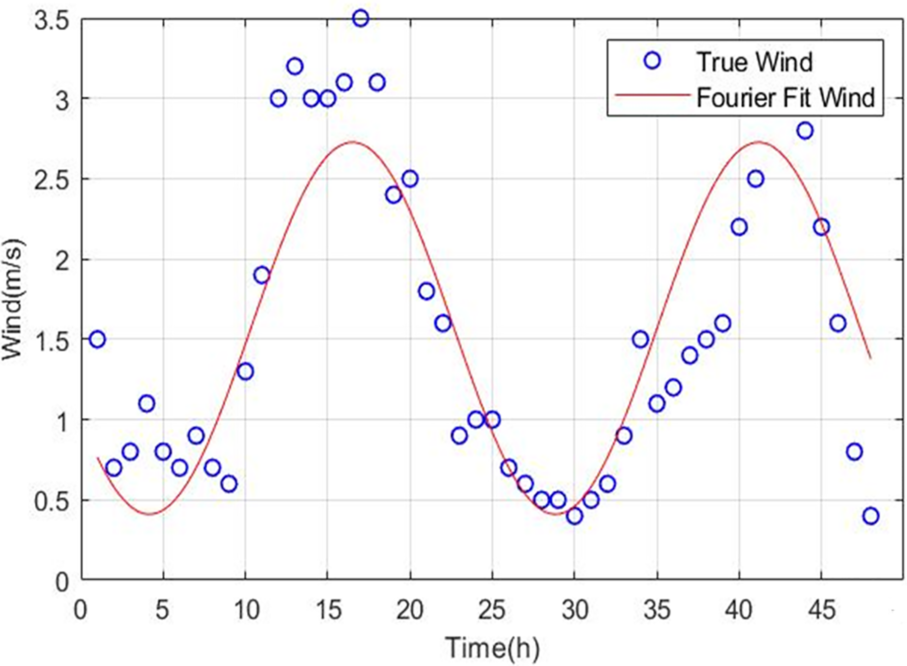
Wind-solar meteorological data exhibit significant seasonal characteristics across multiple time scales, including daily, weekly, monthly, seasonal, and annual. Taking wind speed time series as an example, periodic fluctuation characteristics at both daily and annual scales can be clearly observed through simple Fourier fitting, as shown in Figs. 3 and 4. Through simple Fourier fitting, periodic fluctuations at daily and annual time scales can be identified.
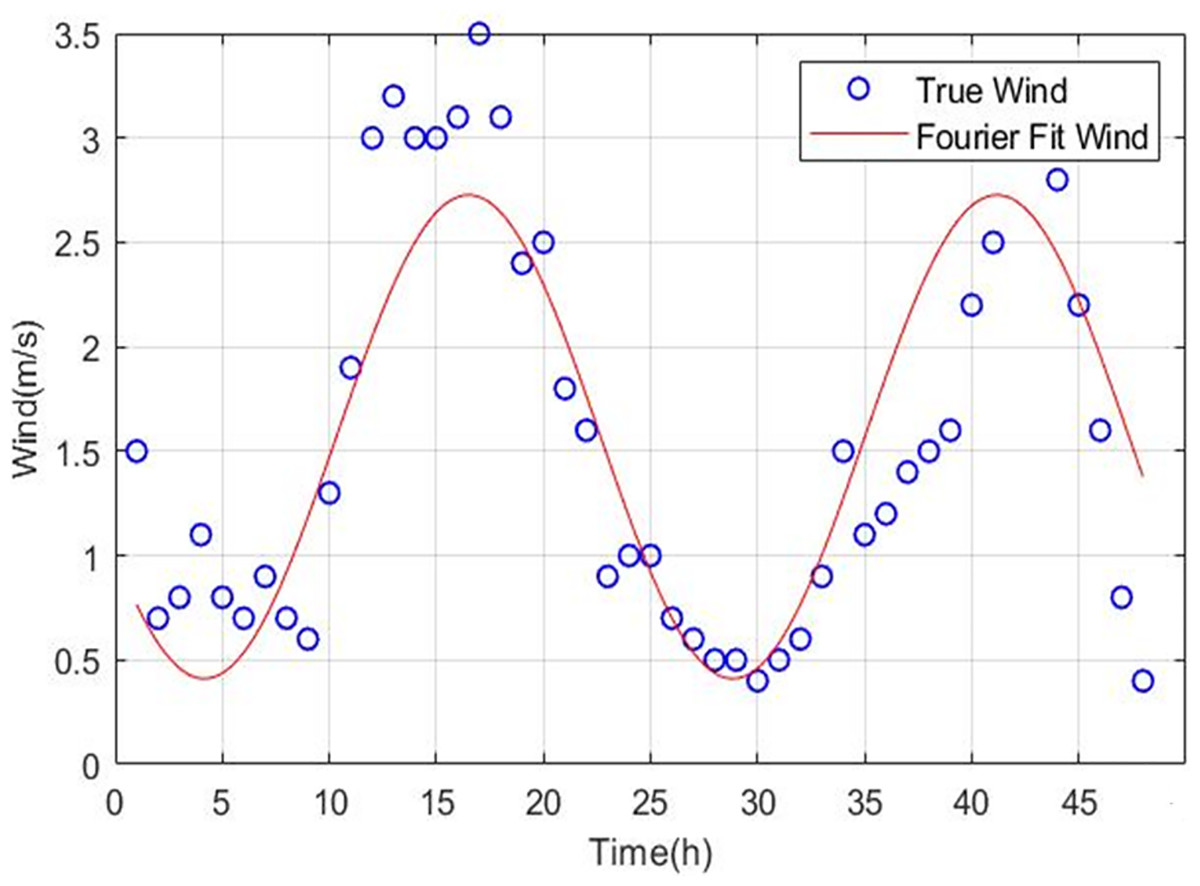
Figure 3: Short-term seasonality of wind speed.
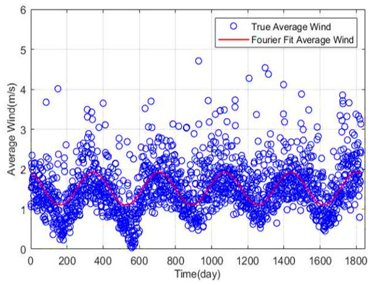
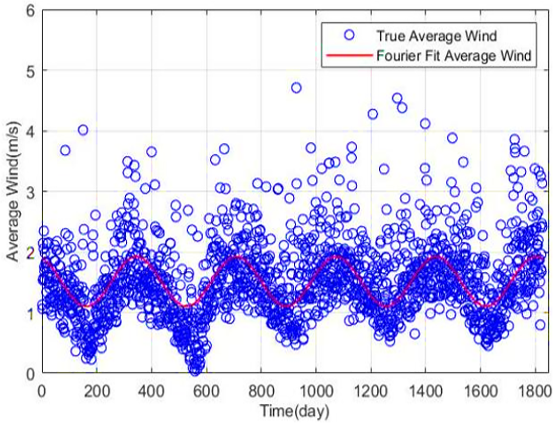
Figure 4: Long-term seasonality of wind speed.
STL-based long-term wind-solar sequence decomposition method
Time series typically comprises four main components: trend, seasonality, periodicity, and random fluctuations:
The trend component reflects long-term variation patterns, exhibiting either linear or nonlinear characteristics.
The seasonal component characterizes regular fluctuations caused by seasonal changes, encompassing multi-scale features, including daily and seasonal cycles.
The residual component represents random fluctuations or noise.
Time series decomposition models can be categorized into additive and multiplicative models. The additive model assumes that components are mutually independent with consistent dimensions; in multiplicative models, the trend component shares the output dimension, seasonal and cyclical components are proportional values, and the residual component follows a normal distribution. This article employs the additive model for STL decomposition.
We set the decomposition period to 1 year (8,760 h) for both wind speed and solar radiation to effectively separate long-term seasonal effects from trend and residual components. This choice is motivated by the strong annual seasonality inherent in both datasets, where Fourier analysis reveals clear daily and annual periodicities in wind speed as shown in Figs. 3 and 4. Solar radiation similarly exhibits pronounced daily and annual cycles due to Earth’s rotation and orbit. While we acknowledge that solar radiation typically follows strong daily and seasonal cycles and wind speed can show more irregular patterns, our STL decomposition with an annual period captures the dominant seasonal cycles relevant for long-term forecasting. This approach simplifies the decomposition while maintaining interpretability and leveraging the strong annual climatic cycles affecting both variables. Although our primary focus was on the annual cycle, we did consider the importance of shorter periods such as daily and weekly cycles. To supplement the STL decomposition, we incorporated additional temporal feature engineering steps, including cyclic encoding of hour of day and day of year and the use of 24-h and 168-h moving averages. These features help capture shorter-term periodicities and variability that are not explicitly decomposed by the fixed annual STL period.
STL decomposition, proposed by Cleveland (1979), is a time series analysis method that decomposes sequence data into three key components: Trend, Seasonal, and Residual. This method effectively reveals the inherent structural characteristics of time series, providing an essential tool for data analysis.
(1) where:
Tt represents the Trend component, indicating the long-term variation trend of the data.
St represents the Seasonal component, indicating periodic fluctuations with fixed cycle lengths.
Rt represents the Residual component, indicating random fluctuations or noise.
The STL decomposition process includes the following iterative steps:
Initial decomposition: smooth the sequence to obtain initial estimates of trend and seasonality.
Seasonal smoothing: after removing the trend, use LOESS to estimate average values at each seasonal position.
Trend smoothing: after removing the seasonal component, use LOESS to estimate new trend components.
Residual calculation: subtract trend and seasonal components from the original sequence.
Iterative optimization: repeat the above steps until convergence.
Although the STL decomposition step applies the same fixed annual period to both variables. The trend component for each variable is modeled using the FEDformer model, which excels in capturing long-term trends and periodic components. The periodic component is modeled separately with an Attention-LSTM network, which is well suited to capture varying periodicities and complex temporal dependencies. By decomposing the time series into trend, seasonal, and residual components and applying specialized models to each, the framework adapts to variable-specific patterns implicitly.
LOESS, also known as LOWESS, is a non-parametric regression technique used to estimate the average trend in data without assuming a specific global functional form (Cleveland, 1979). It works by fitting simple local models (typically linear or quadratic) to subsets of the data, weighted by proximity, allowing it to capture complex, nonlinear patterns in noisy datasets. In the time series analysis, LOESS is particularly useful for smoothing and identifying long-term trends by locally adapting to the structure of the data. This makes it well-suited for applications like wind speed or solar radiation trend estimation, where global models may fail to capture localized fluctuations (Hewamalage, Bergmeir & Bandara, 2021).
Long-term time series prediction model based on hybrid deep learning
LSTM neural network structure
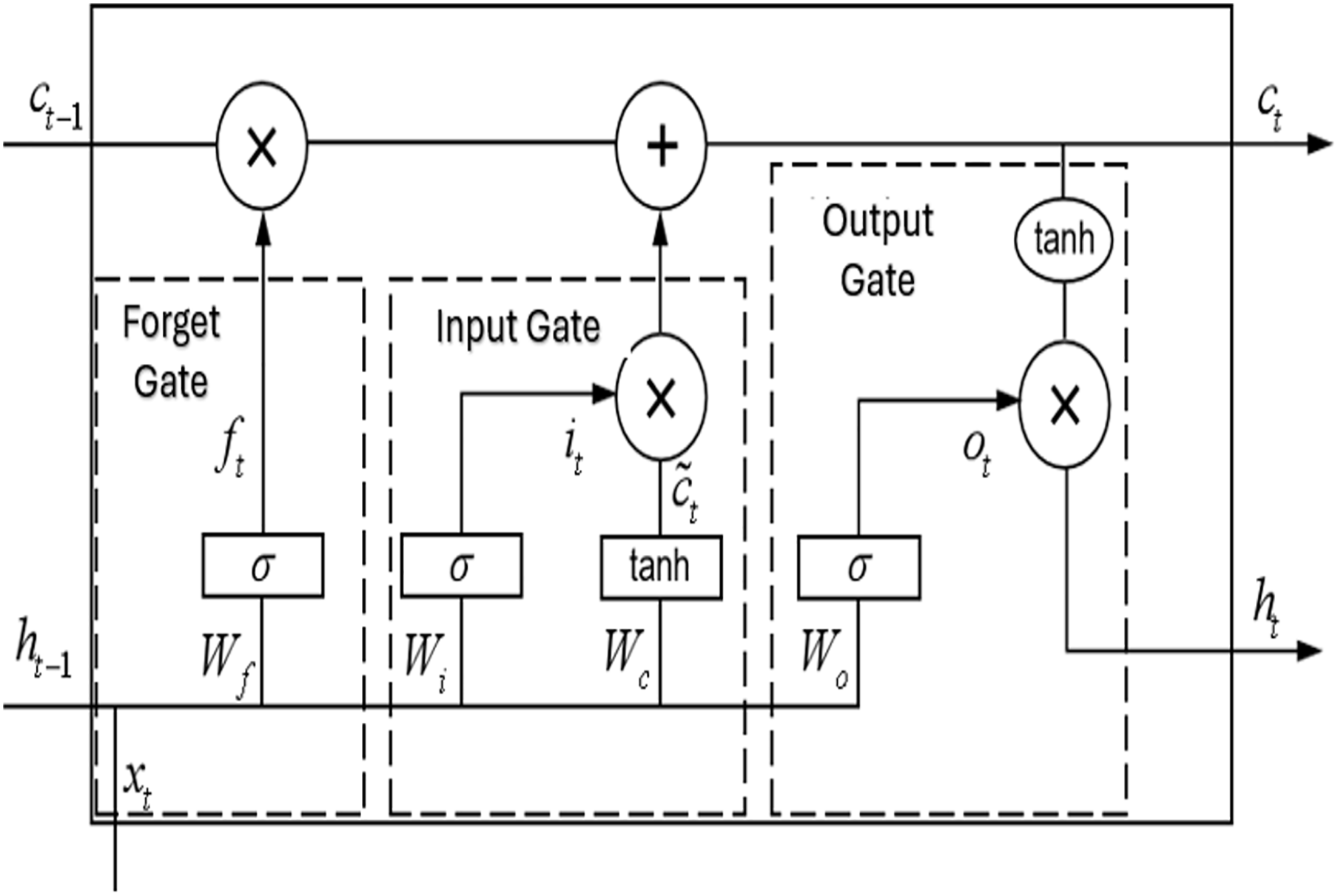
Long Short-Term Memory (LSTM) networks, as a special type of recurrent neural network (Wang et al., 2021), have a unit structure as shown in Fig. 5. Each LSTM unit contains a cell state and three gate units (forget gate, input gate, and output gate). LSTM can effectively learn long-term dependencies through this gating mechanism, overcoming the vanishing and exploding gradient problems of traditional recurrent neural networks (RRNs), and demonstrating superior performance in long-term sequence prediction.
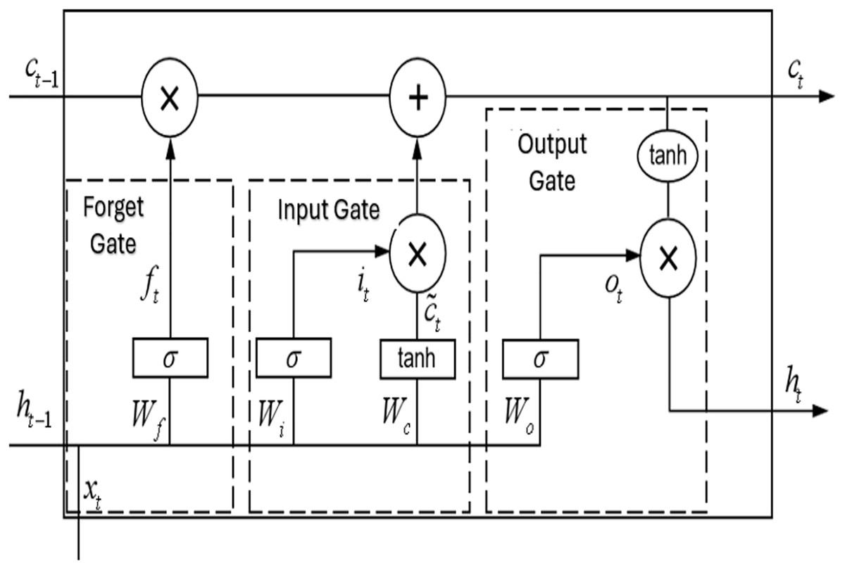
Figure 5: Structure diagram for LSTM cell.
In LSTM networks, the input consists of the current time step input vector , the previous time step hidden layer output vector , and the cell state . The output includes the current time step output vector and the cell state . Here, , , and represent the activation vectors of the forget gate, input gate, and output gate, respectively, with denoting the sigmoid activation function.
The forget gate determines the degree of information retention in the cell state through a sigmoid function. It receives the previous hidden state and current input, outputting a vector with values in the range , where 0 indicates complete forgetting and 1 indicates complete retention. Its equation is:
(2) where:
is the forget gate;
represents the sigmoid activation function;
and are the weight matrix and bias vector, respectively;
is the unit output at time step ;
is the information input at time step .
The input gate controls the update of new information. The sigmoid layer output determines the update content, while the tanh layer generates candidate value vectors . Their combination determines the cell state update. The expressions are:
(3)
(4)
(5) where, represents the cell state at the previous time step ; , , and are learnable parameters.
The output gate regulates the information flow from the cell state to the hidden state . It is expressed as:
(6)
(7) where: ot is the activation vector of the output gate, with Wo and bo being learnable weight and bias parameters.
Attention mechanism
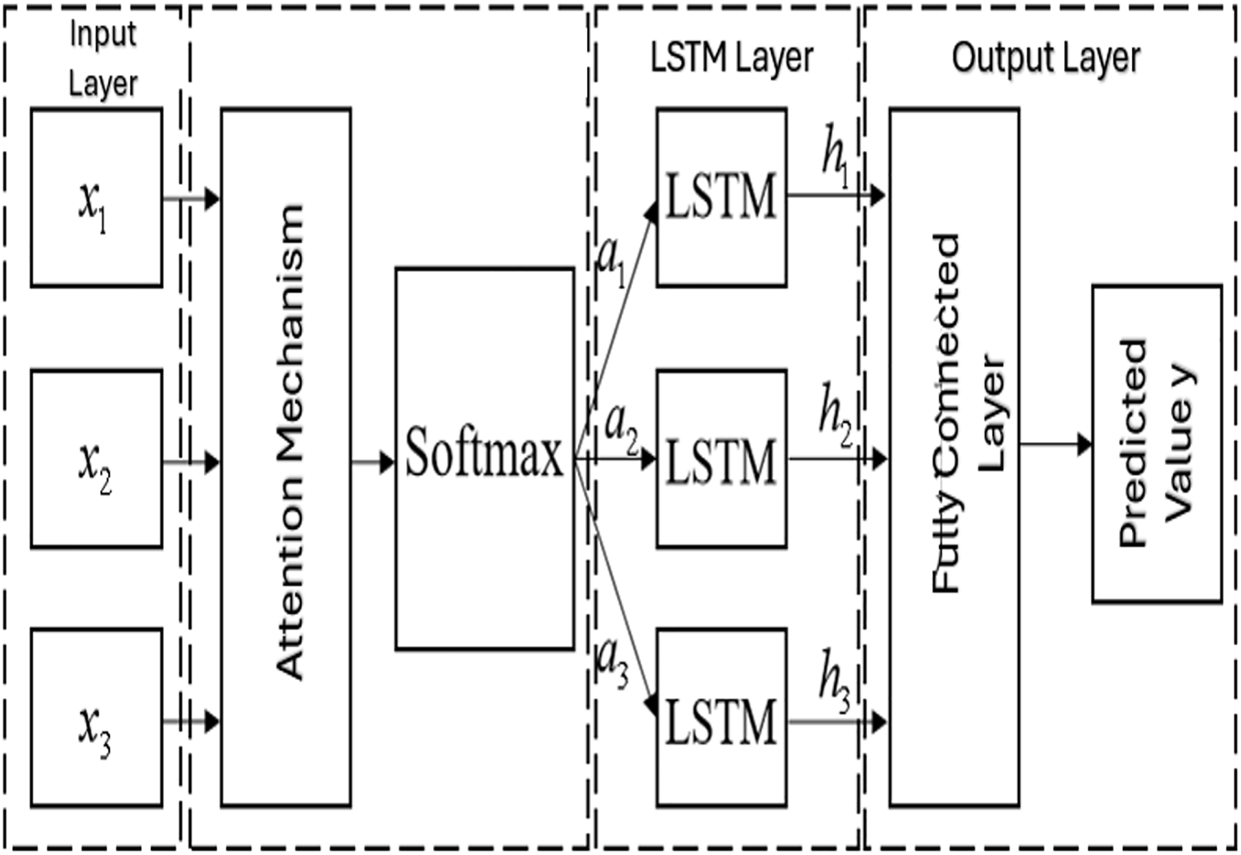
The attention mechanism (Zhang et al., 2021) is a deep learning technique inspired by human visual cognition that enables models to focus on key information within input sequences adaptively. This mechanism has significantly enhanced models’ capability to process long sequence data in sequence processing tasks. This article combines the attention mechanism with LSTM networks to enhance the model’s capture of sequence data features. The mechanism achieves dynamic weight allocation across input sample dimensions through iterative loss function optimization. During training, the model dynamically adjusts input dimension weights through backpropagation based on prediction errors, thus achieving an adaptive assessment of feature importance. This approach improves the model’s ability to identify key information and enhances model interpretability.
In the specific implementation as shown in Fig. 6, the attention mechanism maintains and utilizes the intermediate state outputs of LSTM layers, establishing correlations with target sequences to learn to assign higher weights to important input features. We can write
(8)
(9)
(10) where:
represents the current time step input sample.
is the feature importance scoring function correlated with prediction output relevance.
quantifies the contribution of input states to current predictions. The model implements attention analysis based on the relative importance between feature dimensions.
is the attention layer output.
and are trainable parameters.
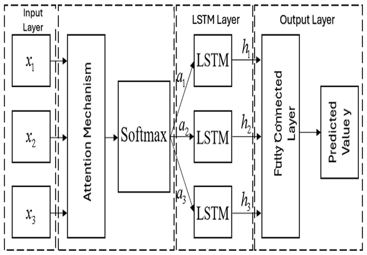
Figure 6: Structural diagram of the LSTM incorporating the attention mechanism.
FEDformer model
FEDformer, as one of the best-performing time series prediction models in the Transformer variant family (Shi et al., 2015), features a core architecture comprising encoder-decoder structure, frequency domain enhancement mechanism, and temporal decomposition mechanism. The model effectively improves global time series modeling capability by integrating frequency enhancement, a mixture of experts, and seasonal-trend decomposition. Our motivation for employing the FEDformer model lies in the nonlinear and non-stationary nature of renewable energy trends, particularly under varying climatic influences. FEDformer extends traditional transformer architectures by incorporating frequency domain attention mechanisms and multi-scale temporal decomposition. These enhancements allow the model to effectively capture subtle, evolving long-term dependencies that may not be readily apparent through conventional time-domain modeling alone. Notably, the trend component extracted through STL decomposition is not strictly linear, it may include low-frequency fluctuations with long-memory effects, gradual structural changes, and multi-year variability due to climate patterns, grid evolution, or urban development.
In the model structure design, FEDformer introduces Fourier enhancement blocks and wavelet enhancement blocks as key Transformer components, replacing traditional self-attention and cross-attention mechanisms with frequency domain mapping to better capture frequency features and essential structures of time series. To optimize computational efficiency, the model randomly selects fixed numbers of Fourier components, achieving linear computational complexity while significantly reducing memory overhead. The FEDformer encoder primarily extracts temporal features from wind-solar sequences, while the decoder generates predicted wind speed and radiation intensity sequences based on encoder outputs. The frequency domain enhancement mechanism enhances temporal information representation through Fourier transformation. The sequence decomposition module (MOE) decomposes input sequences into trend and periodic components, with the encoder processing only periodic information while the decoder adds trend components to periodic ones to obtain final predictions. Residual connections are employed between modules to prevent gradient vanishing. The overall model architecture is shown in Fig. 7.
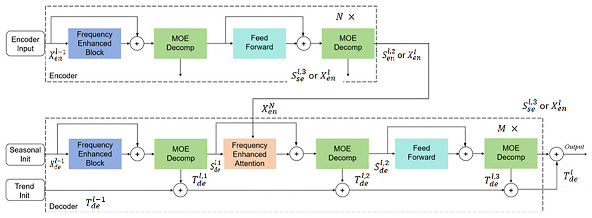
Figure 7: FEDformer model structure.
The encoder of FEDformer adopts a multi-layer structure, as shown in Fig. 8, with its computation process defined as follows:
where represents the historical time series data. After normalization and embedding into suitable dimensions for the model input , it serves as the encoder’s input. The input data sequentially passes through the frequency domain enhancement module, sequence decomposition module, and feed-forward neural network. The frequency domain enhancement module extracts important sequence features. This is followed by the sequence decomposition module, which decomposes seasonal components. The feed-forward neural network then performs fully connected operations. The specific equations for these operations are as follows:
(11)
(12)
(13) where:
, represents the -th seasonal component in the -th layer.
The frequency domain enhancement module calculates attention in the frequency domain through Fourier transform and wavelet transform.
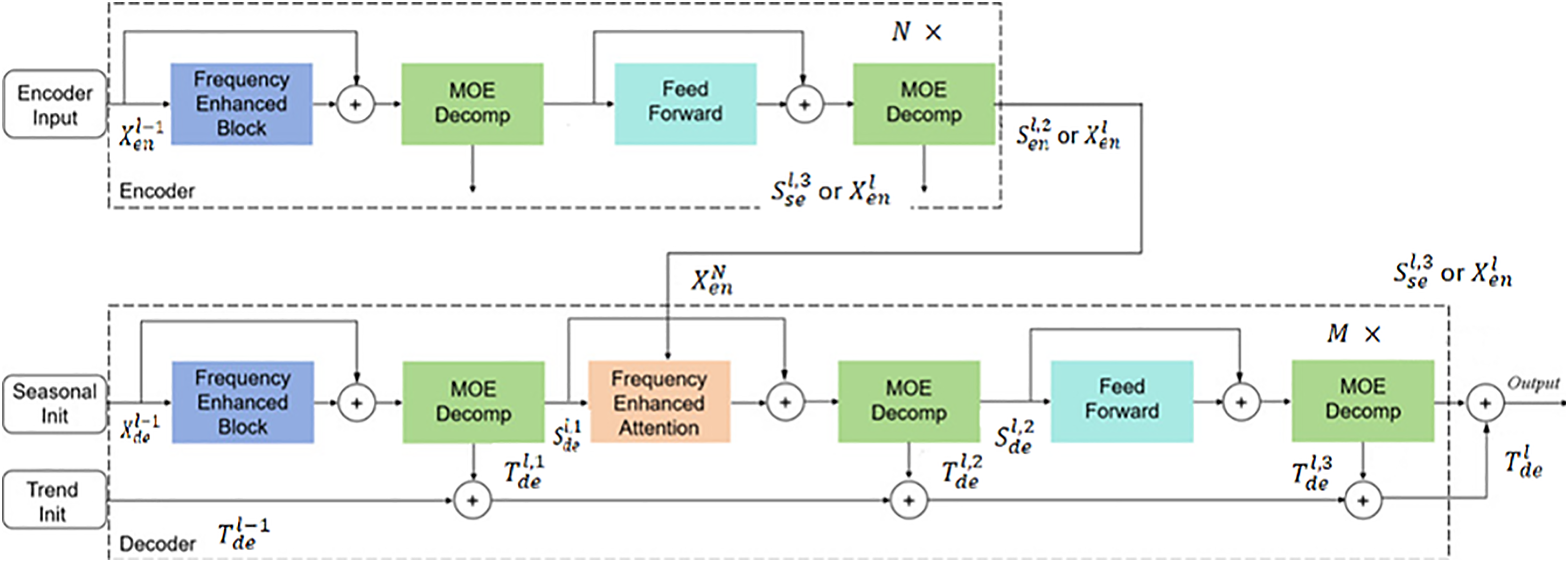
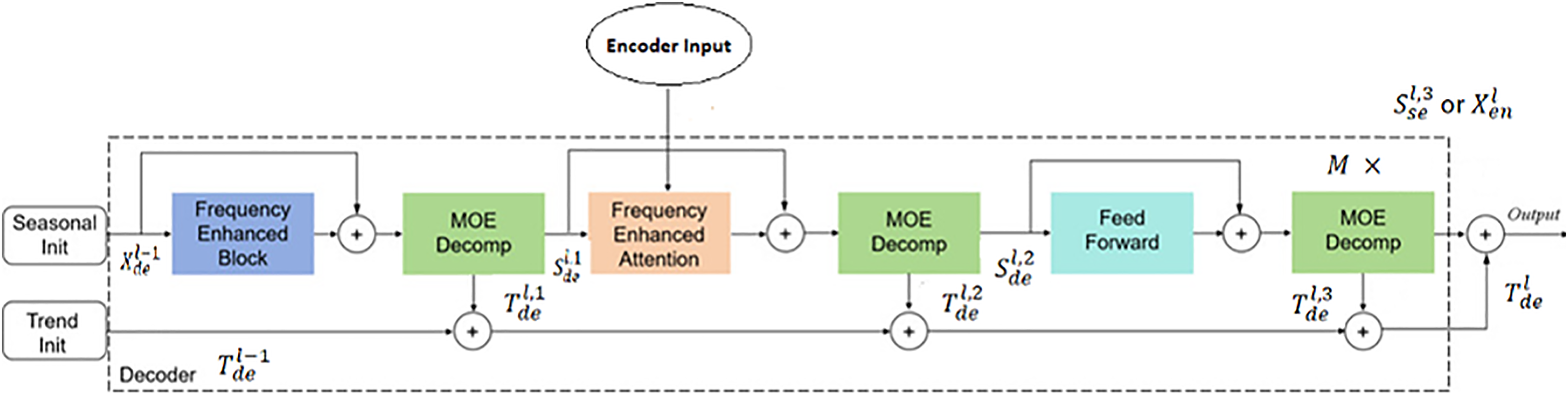
The decoder also employs a multi-layer structure, as shown in Fig. 9. It is defined as:
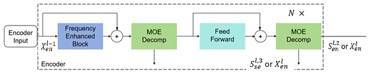
Figure 8: Encoder structure.
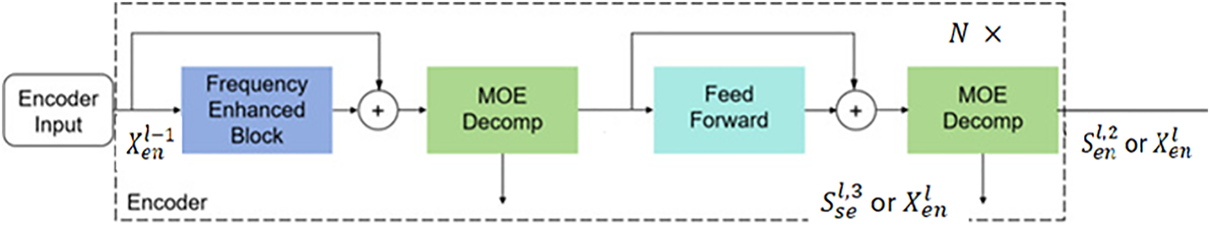
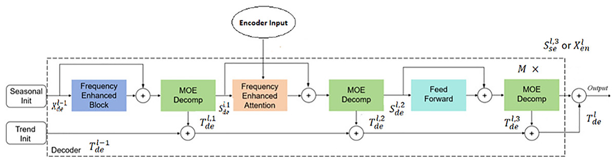
Figure 9: Decoder structure.
In contrast to the encoder, the decoder processes both seasonal and trend components. Seasonal components are sequentially added to the decoder’s output through various frequency domain enhancement mechanisms. Trend components are continuously accumulated to increase information utilization. We can write
(14)
(15)
(16)
(17)
(18)
The frequency domain enhancement mechanism consists of the Frequency Enhancement Block (FEB) and Frequency Enhancement Attention (FEA). This article employs Fourier transform for frequency domain conversion. Frequency Enhancement Block (FEB) transforms the input sequence into the frequency domain using the Fourier transform, where it applies attention mechanisms to selectively enhance informative frequency components. Even though the STL-trend is low-frequency by nature, FEB can identify subtle harmonic variations and enhance weak but relevant frequency signals, such as multi-seasonal cycles, inflection points, or slow shifts, thus refining the input for better prediction. The inverse transform then restores the enhanced sequence to the time domain, with critical frequency components now emphasized.
In FEB, time series data is first mapped to the frequency domain through Fourier transform, followed by random sampling of frequency domain information with zero-padding to maintain dimensionality, and then returned to the time domain through inverse transform to obtain enhanced sequences. The mathematical expressions are:
(19)
(20) where, represents retaining M-dimensional sequence information in an N-dimensional sequence , represents Fourier transform, represents inverse Fourier transform, R is a randomly initialized parameter kernel, represents padding the retained M-dimensional information with zeros to N dimensions.
The FEA mechanism innovatively combines Fourier transform with attention mechanism, enhancing sequence features by computing attention weights in the frequency domain. This mechanism can replace traditional cross-attention modules, improving sequence modeling performance. The implementation process involves mapping input sequences to the frequency domain through one-dimensional Fourier transform, computing frequency domain attention weights, and returning to the time domain through inverse transform to obtain enhanced sequences. The mathematical expressions are:
(21)
(22)
(23)
(24) where q, k, v represent query, key, and value respectively, represent the activation function.
Mixture-of-Experts Decomposition (MOEDecomp) applies average filters of varying kernel sizes to decompose the input trend further into multi-resolution temporal components. Unlike STL, which performs fixed decomposition based on user-defined seasonality, MOEDecomp provides learned, data-driven decomposition that adapts during training. It extracts both short-range and long-range smooth components, enabling the model to better represent compound patterns in the trend, including those that may not have been fully captured by STL alone. The MOEDecomp decomposition module differs from common fixed-window decomposition. This module decomposes the input sequence into seasonal and trend components through a set of average filters of different sizes, highlighting long-term sequence trends. The specific representation is as follows:
(25)
(26) where Softmax denotes the weights used to mix the extracted trend components, and AvgPooling represents the average pooling operation applied to the input sequence .
Evaluation of FEDformer model
We have compared the performance of FEDformer model with classical forecasting approaches such as exponential smoothing (Alnaa & Ahiakpor, 2011), AutoRegressive Integrated Moving Average (ARIMA) (Bailey et al., 2021), and polynomial regression (Hyndman & Athanasopoulos, 2018), as reported in Table 3.
| Model | RMSE |
|---|---|
| ARIMA (Bailey et al., 2021) | 0.611 |
| Exponential smoothing (Alnaa & Ahiakpor, 2011) | 0.385 |
| Polynomial regression (Hyndman & Athanasopoulos, 2018) | 0.407 |
| FEDformer | 0.354 |
An ablation study was conducted to evaluate the effectiveness of the FEDformer model compared to simpler forecasting methods like ARIMA, exponential smoothing, and polynomial regression for predicting the trend component of solar radiation. The performance was assessed using root mean square error (RMSE). The FEDformer model achieved the lowest RMSE of 0.354, indicating the highest accuracy among the tested models. Exponential smoothing and polynomial regression followed with RMSE values of 0.385 and 0.407, respectively, while ARIMA performed the least effectively with an RMSE of 0.611. These results support the use of FEDformer for modeling complex, long-term trend behaviors, demonstrating its superior ability as compared to statistical methods.
Experimental setup and results
The preprocessing pipeline addresses several key challenges inherent in meteorological time series data while preparing it optimally for deep learning analysis. Missing value treatment forms the foundation of our preprocessing strategy. Short gaps under 6 h are handled through linear interpolation, preserving local temporal patterns while maintaining data continuity. For medium-length gaps extending up to 48 h, we employ a 24-h moving average window, which captures daily cyclical patterns to provide more robust estimates. This approach balances the need for data completeness with statistical reliability. However, segments with persistent missing data exceeding 48 h are excluded to prevent the introduction of potentially unreliable synthetic data.
The temporal processing phase standardizes the data structure to facilitate model training. Raw data is resampled to consistent hourly intervals using mean aggregation, ensuring uniform temporal spacing. Time zones are standardized to UTC+12 to align with New Zealand local time, critical for capturing local meteorological patterns. Each annual sequence is standardized to 8,760 points, creating a structured foundation for the STL decomposition process.
The rationale behind for choosing a 24-h window stems from the strong daily cyclical patterns typical in meteorological variables such as wind speed and solar radiation. Using this window aims to leverage the natural diurnal cycle to provide robust gap-filling estimates that are more consistent with underlying periodic behavior, rather than arbitrary interpolation methods which might introduce unrealistic short-term fluctuations. Regarding the 48-h threshold for excluding longer gaps, this cutoff was selected to balance data completeness with reliability. Missing segments beyond 48 h tend to be less predictable and risk introducing spurious data that could degrade model training quality. The dataset is available at https://doi.org/10.5281/zenodo.15621883.
Feature engineering significantly enhances the model’s ability to capture temporal patterns. The STL decomposition, applied with 8,760 h, effectively separates the time series into trend, seasonal, and residual components, enabling the model to learn patterns at different time scales. Cyclic encoding of temporal features–converting hour of day and day of the year into sine and cosine components—preserves the circular nature of these time patterns. The addition of 24-h and 168-h moving averages captures both daily and weekly trends, providing the model with important historical context. The input dimension of 8,760 × 5 refers to hourly data for each of five distinct years, yielding 8,760 h per year (excluding leap years). However, in the training phase, we used data from the 4-year period of 2019 to 2022 exclusively, reserving the year 2023 for testing and evaluation. Therefore, while the total dataset spans 5 years (2019–2023), only 4 years are utilized for training to ensure an unbiased assessment of model performance on unseen data.
Quality control measures ensure data reliability while respecting physical constraints. The 3σ rule identifies and removes statistical outliers while preserving natural variations. Physical constraints which limit wind speed to 0–50 m/s and solar radiation to 0–1,500 W/m2, maintain real-world feasibility. Adjacent time step consistency checks identify and correct anomalous jumps in values, ensuring temporal coherence. Finally, min-max normalization scales all features to the [0, 1] range, optimizing the numerical stability of the deep learning process while preserving relative relationships between values.
Parameter settings
Hyperparameter selection for both FEDformer and Attention-LSTM was performed using a combination of manual tuning and systematic grid search. Initially, a broad grid search was conducted over key parameters such as learning rate, batch size, number of layers, and hidden units based on guidelines from previous studies and model documentation. For each model, we defined a search space for critical hyperparameters, including:
FEDformer: learning rate ∈ {0.0001, 0.0005, 0.001}, number of encoder layers ∈ {2, 3, 4}, attention heads ∈ {4, 8}, and kernel size for MOEDecomp ∈ {3, 5, 7}. The FEDformer model configuration includes one encoder and one decoder, an eight-head self-attention mechanism, input sequence length of 8,760 × 5 (corresponding to 5 years of historical data), and output sequence length of 8,760 (corresponding to 1-year prediction).
Attention-LSTM: number of LSTM layers ∈ {1, 2}, hidden units ∈ {64, 128, 256}, and dropout ∈ {0.1, 0.2, 0.3}. Model parameters are configured as follows: hidden layer dimension 128, feed-forward network layer dimension 512, and Adam optimizer learning rate 10-5. The dataset was split into training, validation, and test sets in a 7:1:2 ratio. The early stopping mechanism (training stops if validation error does not decrease for three consecutive epochs) was implemented to prevent overfitting. RMSE was used as the loss function with a batch size of 1,024. The Attention-LSTM model configuration includes 150 training epochs, batch size 64, LSTM hidden layer dimension 256, 8 attention heads, and RMSE loss function. All experiments were repeated three times with averaged results. Detailed parameter configurations are shown in Table 4.
| Parameter | Description | Value |
|---|---|---|
| lr | Learning rate | 0.00001 |
| batch | Batch size | 1,024 |
| freq | Data time scale | h (hour) |
| pre_len | Prediction length | 8,760 |
| Hid_F | FED hidden layer | 512 |
| Hid_L | LSTM hidden layer | 256 |
| F_epo | FED training epochs | 10 |
| L_epo | LSTM training epochs | 150 |
| De_cy | Data decomposition cycle | 8,760 |
We used a 5-fold time series cross-validation on the training dataset to evaluate the performance of different parameter sets based on validation RMSE. Once promising configurations were identified, we performed manual fine-tuning to balance training stability and computational efficiency, particularly when training FEDformer on long sequences (e.g., 8,760-h yearly data).
Performance comparison analysis
The model was validated using wind speed and radiation intensity data from Auckland Meteorological Station, New Zealand, spanning 2019–2023, with data from 2019–2022 used for training and 2023 data for testing at hourly sampling intervals. We employed five statistical indicators, mean absolute error (MAE), mean squared error (MSE), RMSE, p-value, and R2–to compare the proposed method against Attention-LSTM (Draper & Smith, 1998), Auxiliary Classifier GAN (ACGAN) (Wen & Li, 2023), and FEDformer (Liu, Li & Zheng, 2025). Attention-LSTM (Draper & Smith, 1998) was chosen to represent recurrent neural network-based architectures, which have been widely adopted for modeling sequential dependencies and are well-suited to capturing long-range temporal patterns, especially when enhanced with attention mechanisms. Given its proven effectiveness in many renewable energy forecasting studies, it serves as a strong benchmark for periodic and cyclical components (Basu, 2023). FEDformer (Liu, Li & Zheng, 2025) was selected as representing a state-of-the-art Transformer-based architecture specifically tailored for long sequence forecasting. Its combination of frequency-domain attention and decomposition mechanisms makes it a powerful model for capturing multiscale temporal features, particularly trend components in renewable energy data. As our proposed approach builds on this architecture, including FEDformer as a baseline provides a direct and fair comparison to highlight the impact of our enhancements. ACGAN (Wen & Li, 2023) was incorporated to evaluate the use of generative approaches in time series prediction, particularly due to its demonstrated ability to model complex, nonlinear patterns and generate realistic synthetic time series. Including ACGAN also helps benchmark our model against adversarial architectures, which are less common but gaining attention in recent literature.
Wind speed prediction comparisons are shown in Table 5, and radiation intensity prediction comparisons are shown in Table 6. The comparative results demonstrate that our proposed method outperforms existing methods across all evaluation metrics, with prediction results better aligned with historical data distribution characteristics. This validates the superiority of the proposed method in long-term wind-solar sequence prediction tasks.
| Metrics | STL-LSTM -FED |
Attention -LSTM |
AC GAN |
FED former |
|---|---|---|---|---|
| MSE | 0.148 | 0.642 | 3.028 | 0.476 |
| RMSE | 0.385 | 0.801 | 1.740 | 0.690 |
| MAE | 0.307 | 0.603 | 1.205 | 0.515 |
| R2 | 0.889 | 0.830 | 0.407 | 0.874 |
| Metrics | STL-LSTM -FED |
Attention -LSTM |
AC GAN |
FED former |
|---|---|---|---|---|
| MSE | 0.105 | 0.284 | 0.805 | 0.094 |
| RMSE | 0.324 | 0.533 | 0.897 | 0.306 |
| MAE | 0.188 | 0.370 | 0.710 | 0.148 |
| R2 | 0.958 | 0.697 | 0.181 | 0.900 |
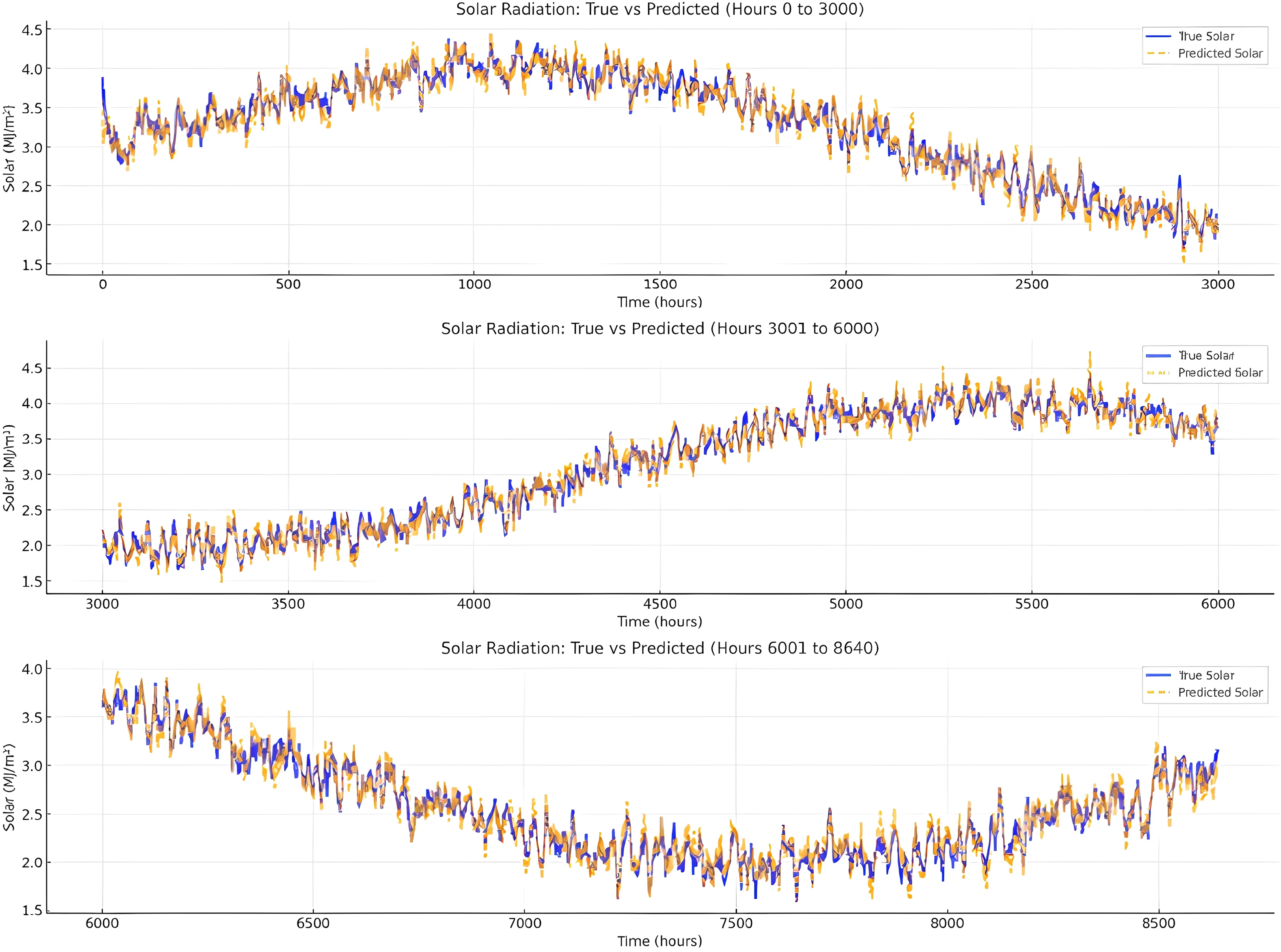
Figure 10 demonstrates a strong correlation between the true solar radiation values and the predicted values, indicating that the model effectively captures the overall trend and seasonal variations in solar radiation. The predicted values closely follow the diurnal and seasonal fluctuations, suggesting that the model successfully learns and replicates periodic patterns in solar energy. The peaks and troughs of the true solar values are well represented, confirming that the model maintains its accuracy across different time periods. While there are minor deviations, particularly in regions with high variability, the overall prediction quality remains consistent, with no significant systematic bias. The alignment between true and predicted values suggests that the model is well-calibrated and capable of handling long-term forecasting effectively.
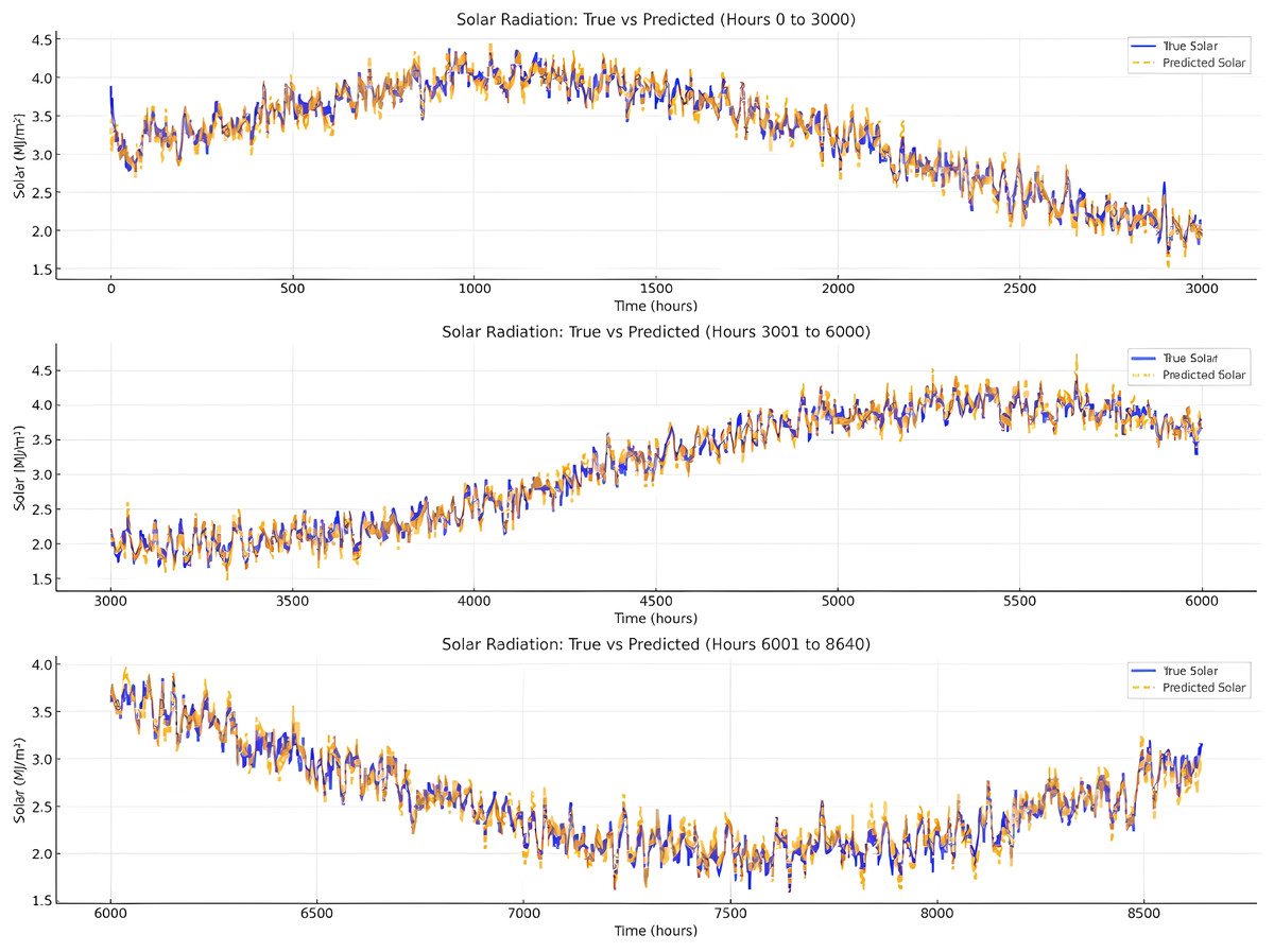
Figure 10: Comparison of the true value/predicted value of the radiation intensity.
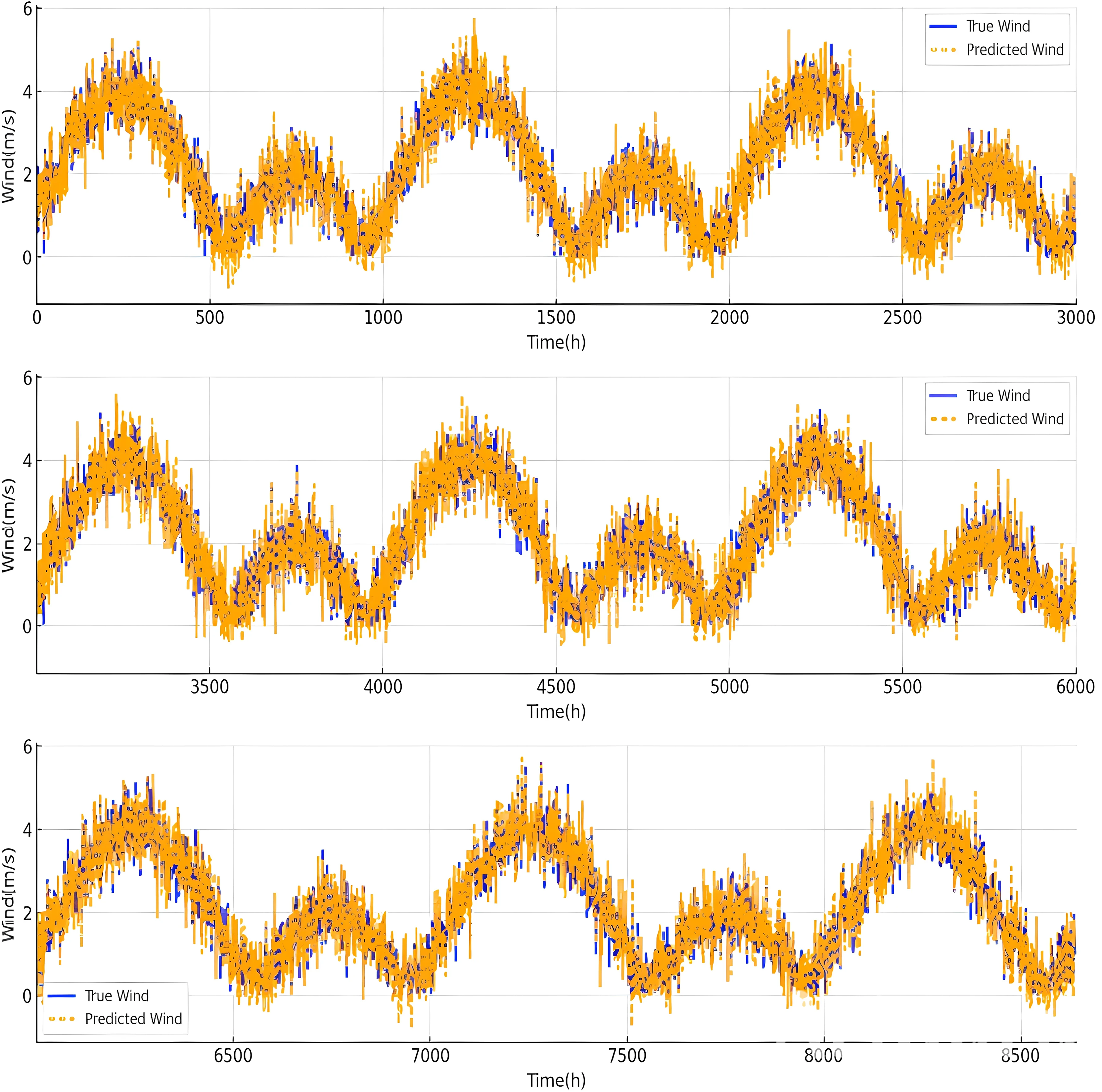
Figure 11 shows the comparison between true wind speed (blue) and predicted wind speed (orange) over time (in hours). The data exhibits high variability and fluctuations in wind speed, with occasional peaks reaching above 6 m/s. The predicted wind values closely follow the true wind values, suggesting that the predictive model performs well in capturing general trends.
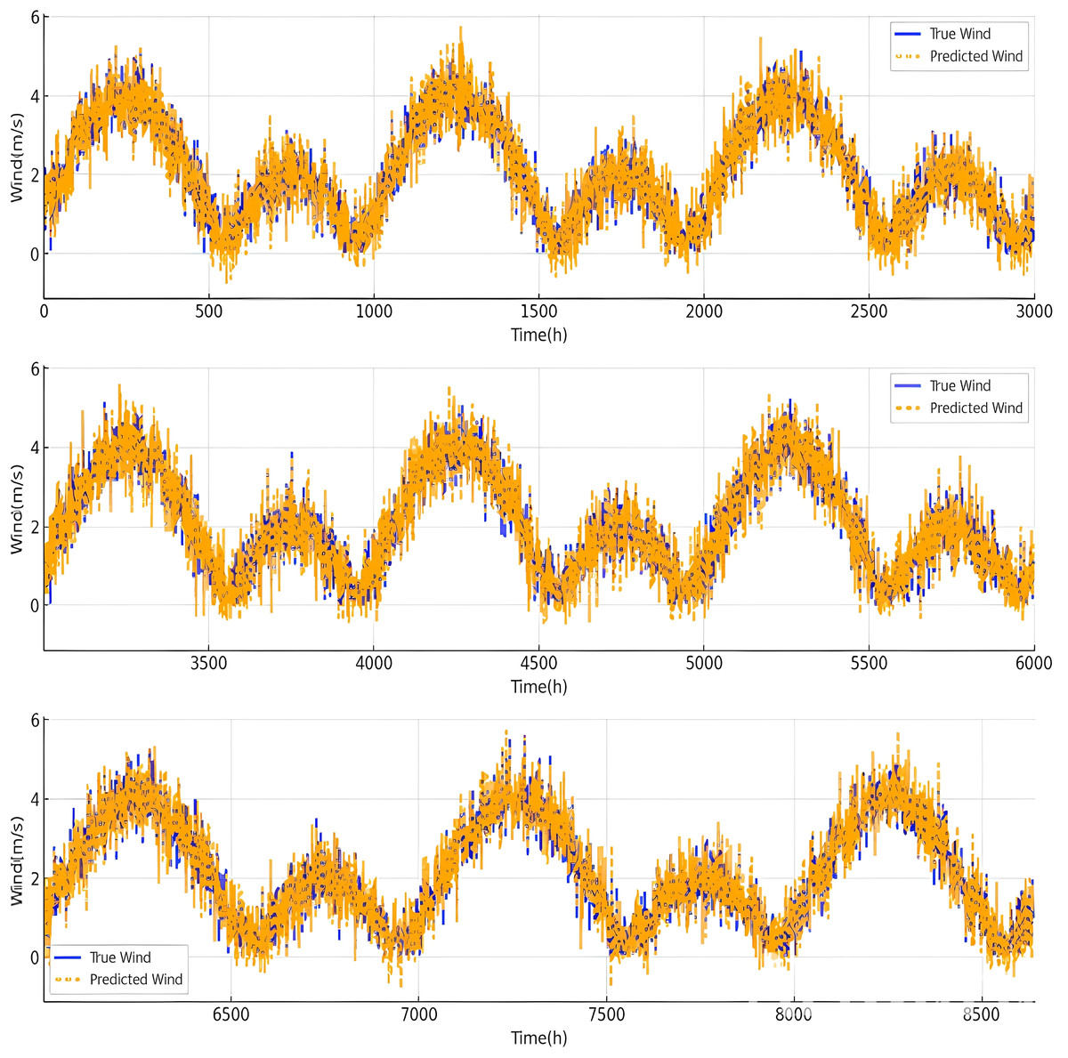
Figure 11: Comparison of the true value/predicted value of the wind speed.
Statistical analysis of proposed model and baselines
To assess the statistical significance of the performance improvements achieved by the proposed STL-LSTM-FED model, paired t-tests were conducted comparing it against three baseline models: Attention-LSTM, AC-GAN, and FEDformer. The resulting p-values are reported in Table 7. All p-values are below the standard significance threshold of 0.05, indicating that the performance improvements of STL-LSTM-FED over each of the baseline models are statistically significant. This suggests that the observed gains in forecasting accuracy are not due to random variation but reflect meaningful and consistent enhancements achieved by the proposed model.
| Model | p-value |
|---|---|
| STL-LSTM-FED vs. Attention-LSTM | 0.0402 |
| STL-LSTM-FED vs. AC-GAN | 0.0446 |
| STL-LSTM-FED vs. FEDformer | 0.0490 |
Conclusions
Addressing the need for long-term prediction of wind-solar sequences, this article proposes the STL-LSTM-FED model. The model comprehensively considers both daily and seasonal characteristics of wind-solar time series, achieving high-precision prediction of long-term wind-solar sequences through accurate modeling of temporal feature correlations. Experimental validation demonstrates that this method outperforms existing approaches in annual wind-solar sequence prediction tasks. In addressing the complex feature correlation challenges in long-term wind-solar prediction, the model innovatively combines attention mechanisms, LSTM, and FED models, generating prediction results by combining trend, periodic, and residual components via adaptive weight adjustment of input features and deep temporal dependency modeling. This design effectively leverages the advantages of each component, significantly enhancing prediction performance.
In future, we can incorporate additional meteorological variables such as temperature, humidity, and atmospheric pressure which could enrich the input data, leading to more accurate predictions. We can also utilize graph neural networks for spatiotemporal data that will capture complex spatial dependencies.