
Sequence-based undersampling: an algorithm for managing imbalanced datasets
- Published
- Accepted
- Received
- Academic Editor
- Martina Iammarino
- Subject Areas
- Algorithms and Analysis of Algorithms, Artificial Intelligence, Data Mining and Machine Learning, Optimization Theory and Computation, Neural Networks
- Keywords
- Imbalance, ML, IA, Regression, Earth sciences, Undersampling
- Copyright
- © 2025 Troncoso et al.
- Licence
- This is an open access article distributed under the terms of the Creative Commons Attribution License, which permits unrestricted use, distribution, reproduction and adaptation in any medium and for any purpose provided that it is properly attributed. For attribution, the original author(s), title, publication source (PeerJ Computer Science) and either DOI or URL of the article must be cited.
- Cite this article
- 2025. Sequence-based undersampling: an algorithm for managing imbalanced datasets. PeerJ Computer Science 11:e3078 https://doi.org/10.7717/peerj-cs.3078
Abstract
Imbalanced datasets pose significant challenges in machine learning (ML), often leading to catastrophic failures in models that are insensitive to their statistical particularities. In regression using neural networks (NN), imbalance is particularly problematic due to the potential undersampling of extreme but important values. Traditional classification methods are ineffective with imbalanced datasets and fail to capture the structure of the problem. This article presents a novel approach to handling imbalanced data in general regression. The new preprocessing technique, called “Sequence-Based Undersampling”, leverages the spatial structure of the data to selectively remove overrepresented instances. The method is tested using quantitative precipitation estimates (QPE), a well-known case of imbalance distribution in earth physics. The technique demonstrates consistent improvements in model performance compared to existing methods. The results suggest that sequence-aware undersampling improves regression models and ML algorithms, providing a practical solution to a prevalent issue in data-driven research. This method can enhance current satellite precipitation algorithms, as satellite retrievals often exhibit a leptokurtic distribution with few cases of high rainfall rates, many low rates, and numerous no-rain occurrences—a paradigmatic case of an imbalanced dataset built sequentially through radar and radiometer measurements.
Introduction
Machine learning (ML) has revolutionized many fields, where accurate predictions are critical for applications such as medicine and biomedicine, computer vision, natural language processing and earth sciences (Jordan & Mitchell, 2015; Reichstein et al., 2019).
In addition to the typical challenges faced by ML (Domingos, 2012), one particular challenge is the handling of imbalanced data, which is a frequent issue in earth sciences applications. The term refers to the statistical distribution (most notably the probability distribution function, or pdf) of the data. Gaussian distributions are common, but skewed distributions such as the Gamma and Log-Normal often feature as a consequence of Poisson processes. This is the case of precipitation data, which is highly skewed towards low precipitation rates: there are far more light than high rainfall rates in a storm, and the same applies to the daily accumulations over a region. This feature makes precipitation data difficult to integrate in ML methods. High rainrates are comparatively scarcer, but critical in meteorological applications as they are indicative of severe weather (Jafarigol & Trafalis, 2023).
Addressing data imbalance is crucial to improve model performance and while several strategies have been developed to address this problem in classification, gradually, these strategies have been adopted and addressed also for regression (Krawczyk, 2016; Branco, Torgo & Ribeiro, 2016).
The challenge of data imbalance is not limited to classification problems; it also significantly impacts regression tasks, where the target variable is continuous. This imbalance can lead to models that fail to adequately capture underrepresented regions of the prediction space, resulting in suboptimal performance. To address this issue, various strategies have been developed. For instance, a recent survey reviews and compares resampling techniques, such as undersampling and oversampling, to improve precision in imbalanced regression scenarios (Avelino, Cavalcanti & Cruz, 2024). Furthermore, advances in deep learning have introduced methods such as label and feature distribution smoothing to handle skewed distributions in regression tasks (Yang et al., 2021). These efforts highlight the importance of developing specialized techniques to tackle the unique challenges posed by imbalance in regression problems.
In this work, a novel preprocessing technique, called Sequence-Based Undersampling (SBU), is proposed to address the data imbalance in regression tasks with sequentially ordered observations. Unlike traditional methods, SBU leverages the natural order in which the data were recorded to selectively remove overrepresented instances, thereby preserving the underlying temporal patterns and reducing bias. This approach addresses key challenges in regression imbalance, such as the preservation of critical sequential dependencies and the avoidance of synthetic data generation, which can distort the original data distribution. Moreover, SBU is designed to be straightforward to implement, requiring minimal computational overhead while effectively balancing the dataset.
In terms of applications, SBU has the potential to improve current satellite precipitation algorithms by providing more accurate predictions of extreme weather events, which are often underrepresented in imbalanced datasets. This advancement aligns with recent efforts by organizations like the European Centre for Medium-Range Weather Forecasts (ECMWF), which has integrated machine learning techniques into their forecasting systems to improve accuracy and efficiency (ECMWF, 2024). Similarly, Google’s weather model, which compares favorably with observations using temperature and geopotential metrics (Lam et al., 2023), highlights the growing importance of ML in atmospheric research.
Precedents
Imbalanced classification: classical and recent approaches
The issue of imbalanced data has been extensively studied in classification tasks (Johnson & Khoshgoftaar, 2019; Zhang et al., 2023), where the target variable is discrete and the class distribution is highly skewed. Foundational studies such as Chawla, Japkowicz & Kotcz (2004), Chawla (2005), He & Garcia (2009) provided systematic analyses of how data imbalance negatively affects learning algorithms, particularly in the detection of minority classes, and surveyed the early landscape of solutions. In response, various strategies have been proposed to improve minority class representation during training, broadly divided into: data-level methods, algorithm-level methods, and hybrid or integrated approaches.
Data-level methods
Resampling strategies address class imbalance by modifying the distribution of training data. These include oversampling (e.g., Random Oversampling, Synthetic Minority Over-sampling Technique (SMOTE) (Chawla et al., 2002), Borderline-SMOTE (Han, Wang & Mao, 2005), Adaptive Synthetic Sampling (ADASYN) (He et al., 2008)), undersampling (e.g., Random Undersampling, Tomek Links (Tomek, 1976), Edited Nearest Neighbour (ENN) (Wilson, 1972)), and combined approaches. Numerous extensions have emerged to enhance these strategies. Synthetic Minority Over-Sampling Technique with Local Outlier Factor (SMOTE-LOF) (Asniar, Maulidevi & Surendro, 2022) incorporates local outlier detection, Synthetic Minority Over-Sampling Technique with Boosting and Noise detection (SMOTE-WB) (Sağlam & Cengiz, 2022) integrates boosting and noise filtering, and Improved Majority Weighted Minority Over-Sampling Technique (IMWMOTE) (Wang et al., 2024) improves upon Majority Weighted Minority Over-Sampling Technique (MWMOTE) (Barua et al., 2014) through adaptive noise elimination and weighting. On the undersampling side, techniques such as BOD-based undersampling (Peng & Park, 2022) and convolutional neural network (CNN)-based undersampling (Fan & Lee, 2021) use proximity and learned representations to guide instance selection.
Algorithm-level methods
These approaches modify the learning algorithm to become cost-sensitive or class-aware. Examples include Focal Loss (Lin et al., 2017) and Logit Adjustment (Menon et al., 2020), which adjust the learning signal to emphasize minority instances. Other widely used strategies include Class-Balanced Loss (Cui et al., 2019), which reweights losses based on the effective number of samples, and Cost-Sensitive Learning (Elkan, 2001), which explicitly incorporates class-specific misclassification penalties.
Hybrid and ensemble-integrated methods
Several recent approaches combine data-level resampling with algorithm-level modifications. These hybrid strategies often integrate sample generation with boosting, weighting, or distributional alignment. For instance, WSMOTE-Ensemble (Abedin et al., 2023) applies weighted oversampling within bagging frameworks, while generative adversarial network (GAN)-based methods such as Wasserstein Conditional GAN Oversampling (Zhou et al., 2025) synthesize realistic minority class examples. Optimal transport-based methods (Gao et al., 2023; Guo et al., 2022) redistribute sample importance through geometric alignment, bridging data and model levels.
The challenge of imbalance in regression
Imbalanced regression refers to predictive tasks in which the distribution of the continuous target variable is skewed, resulting in under-representation of certain value regions, typically extremes or areas of high importance. Unlike classification, where imbalance is defined over discrete classes, regression requires additional mechanisms to define what constitutes a “rare” or “relevant” value (Krawczyk, 2016).
To address this challenge, the most widely adopted approach relies on relevance functions—continuous mappings that assign an importance score to each target value based on domain knowledge or statistical heuristics (Branco, Torgo & Ribeiro, 2017). These functions are typically normalized to the [0, 1] range and allow the identification of critical target regions without discretizing the continuous space. Higher values correspond to rare or high-importance regions, while lower values are associated with common, low-impact areas. Relevance functions are used not only to guide resampling decisions but also to evaluate models through relevance-aware performance metrics (Avelino, Cavalcanti & Cruz, 2024), enabling a nuanced handling of imbalance in continuous prediction tasks.
Data-level approaches for imbalanced regression
Resampling methods that operate directly at the data level are commonly used to mitigate imbalance in regression tasks. These techniques aim to adjust the training distribution by adding or removing instances, without modifying the learning algorithm itself.
Oversampling methods include Random Oversampling (He & Garcia, 2009), Gaussian Noise Injection (Menardi & Torelli, 2014), SMOTE for Regression (Torgo et al., 2013), Synthetic Minority Over-Sampling Technique for Regression with Gaussian Noise (SMOGN) (Branco, Torgo & Ribeiro, 2017), and k-Nearest Neighbors Oversampling for Regression (KNNOR-Reg) (Belhaouari et al., 2025), synthesize new samples in regions deemed relevant, based on interpolation, noise perturbation, or neighborhood-based weighting. A recent focused review by Belhaouari et al. (2024) discusses several oversampling strategies for imbalanced regression and highlights the broad algorithmic space available for the generation of synthetic instances.
In contrast, undersampling methods focus on removing instances from overrepresented regions. Their design space is inherently narrower, as the task reduces to identifying and eliminating redundant or low-relevance values. Most techniques follow one of a few paradigms: random elimination, neighborhood disagreement, or rule-based filtering. Classical examples include Random Undersampling (He & Garcia, 2009), ENN, Tomek Links, and CNN, while more recent efforts like Selective Under-Sampling (SUS) (Aleksic & García-Remesal, 2025) represent attempts to formalize instance selection heuristics. Compared to oversampling, there have been fewer methodological developments in pure undersampling for regression, largely due to the conceptual simplicity of the problem. In addition to these strategies, hybrid approaches that combine both oversampling and undersampling have also been proposed. One notable example is the Weighted Relevance-based Combination Strategy (WERCS) (Branco, Torgo & Ribeiro, 2019), which adjusts the instance distribution by probabilistically duplicating highly relevant observations while removing less relevant ones, based on continuous relevance scores.
Table 1 provides a summary of representative data-level resampling techniques for regression, categorized by type and approach.
| Method | Type | Approach |
|---|---|---|
| Random Oversampling (He & Garcia, 2009) | Oversampling | Random instance duplication |
| SMOTE for Regression (Torgo et al., 2013) | Oversampling | Interpolation |
| SMOGN (Branco, Torgo & Ribeiro, 2017) | Oversampling | Interpolation + Noise |
| Gaussian Noise (Menardi & Torelli, 2014) | Oversampling | Noise injection |
| KNNOR-Reg (Belhaouari et al., 2025) | Oversampling | Distance-weighted averaging |
| WERCS (Branco, Torgo & Ribeiro, 2019) | Hybrid | Relevance-weighted resampling |
| Random Undersampling (He & Garcia, 2009) | Undersampling | Random instance reduction |
| ENN (Wilson, 1972) | Undersampling | Neighbor disagreement |
| Tomek Links (Tomek, 1976) | Undersampling | Borderline cleaning |
| CNN (Hart, 1968) | Undersampling | Prototype selection |
| SUS (Aleksic & García-Remesal, 2025) | Undersampling | Rule-based instance selection |
| SBU (This work) | Undersampling | Sequence-aware value filtering |
Note:
Although SMOGN implementations often incorporate random undersampling (RU) as a complementary step to improve class balance, in this work SMOGN is considered a pure oversampling method, emphasizing its primary contribution: the generation of synthetic instances in relevant regions.
Sequence-aware resampling strategies
Most resampling techniques, whether for classification or regression, assume that instances are independent and identically distributed, regardless of the order in which they were recorded. This limits their applicability in datasets where structural or sequential patterns are intrinsic to the data distribution.
An important precedent is the work by Moniz, Branco & Torgo (2017), which explores adaptations of oversampling strategies for time series forecasting. Their methods incorporate temporal constraints to avoid disrupting the autocorrelation structure of sequential data. However, their focus lies in predictive modeling of time-dependent targets, using synthetic data generation, and does not address the problem of instance elimination within structurally redundant patterns.
In contrast, this work addresses a different scenario commonly found in environmental data, such as precipitation estimates: the overrepresentation of a single value (zero) occurring in long, homogeneous sequences. While the dataset includes timestamp information, the structure exploited by the proposed method does not rely on temporal features or patterns, but rather on the simple order in which the values were recorded. Any consistent indexing that preserves the original measurement order is sufficient. These repeated sequences often contain limited informational gain when observed exhaustively, making them suitable candidates for structured reduction.
Existing undersampling methods remove overrepresented values based on statistical or geometric heuristics, treating each instance in isolation. The Sequence-Based Undersampling (SBU) algorithm introduces a different perspective: it considers the structure of consecutive identical values and selectively reduces redundancy by eliminating subsets of these repeated sequences. No previous method in the literature has been identified that explicitly addresses this type of structure-aware undersampling in regression tasks.
Alternative strategies: algorithmic and hybrid approaches
Aside from data-level resampling, several methods address imbalance through algorithmic adaptation or hybrid integration. These include Label Distribution Smoothing (LDS) and Feature Distribution Smoothing (FDS) (Yang et al., 2021), which regularize prediction distributions, as well as Balanced Mean Squared Error (MSE) (Ren et al., 2022) and DenseLoss (Steininger et al., 2021), which reweight the loss to emphasize rare target regions.
Hybrid strategies combine resampling with ensemble learning or loss adjustment. Examples include relevance-guided ensembles like REsampled Bagging (REBAGG) (Branco, Torgo & Ribeiro, 2018) and weighted oversampling with bagging, as in WSMOTE-Ensemble (Abedin et al., 2023). While effective, these methods operate under different assumptions and typically require model-specific adaptation. In contrast, the present work emphasizes a simple, interpretable data-level approach designed for temporally structured imbalance.
Methods
This section provides a concise analysis of the dataset used for demonstrating the concept, as well as an overview of the libraries, algorithms and techniques implemented to achieve the goal.
Dataset description
Passive microwave (PMW) sensors onboard satellites can measure the natural microwave radiation emitted by the Earth’s surface and atmospheric particles (Ulaby, Moore & Fung, 1982). PMW data are crucial for quantitative precipitation estimation (QPE) because electromagnetic radiation at microwave frequencies can penetrate clouds, allowing for more direct observation of precipitation that is possible using infrared frequencies. A more direct use of microwave data is through radar, as the radar reflectivity of hydrometeors is proportional to rainrate. The Core Observatory (CO) of NASA’s Global Precipitation Measurement (GPM) mission combines PMW data from the GPM Microwave Imager (GMI) sensor with radar data from the Dual-frequency Precipitation Radar (DPR) instrument, aiming to provide a global precipitation monitoring of the planet (Skofronick-Jackson et al., 2017) and thus advance climate research. A number of radiometers onboard other satellites complement the CO.
Data for this study come from the GPM constellation. It consists of six variables: five representing the radiometer measurements in five microwave channels and one corresponding to the radar estimate of precipitation from the US Multi-Radar/Multi-Sensor (MRMS) surface radar data, which is deemed as the truth. The data is publicly accessible through NASA’s Precipitation Processing System (PPS). The subset used to test the method contains approximately 7 million records spanning from January 2018 to December 2019 (Troncoso, 2024).
The PMW retrievals are floating-point measurements ranging from 100 to 300 K, representing the brightness temperatures at microwave frequencies. The target variable, instantaneous precipitation, ranges from 0 to 80 mm. The dataset includes the geographic location and the observations time, providing both spatial and temporal information to the measurements.
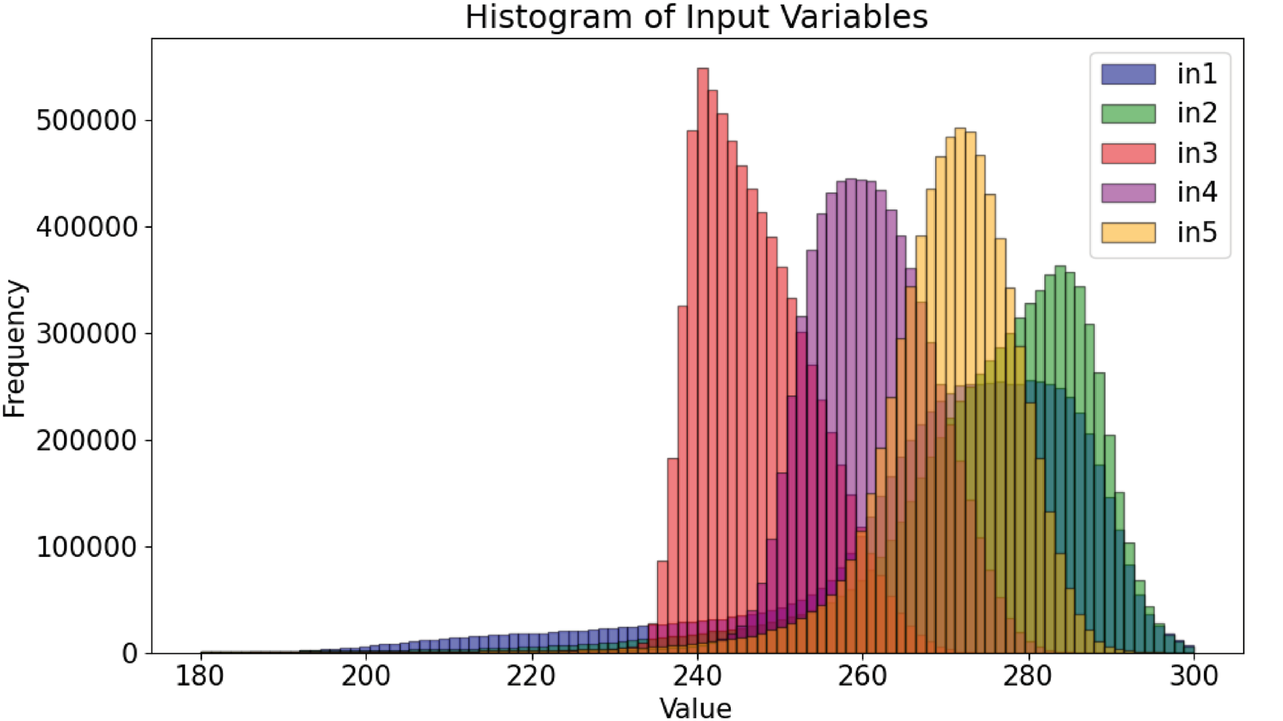
Figure 1 shows the histograms of the microwave radiances (input variables). The five channels approximate a normal distribution. In contrast, the precipitation distribution for the target variable, shown in Fig. 2, indicates that the majority of values are 0.0, representing no precipitation. This feature is well-known in precipitation science, where most algorithms that fuse PMW and radar data first screen for rainy pixels before estimating the actual precipitation quantity. However, even after removing the zeroes, the distribution remains imbalanced, with most cases corresponding to low rain rates. High rain rates are not scarce but are sparsely distributed. Moderate rates, which are crucial for agricultural and environmental studies, fall within the slope of a gentle leptokurtic distribution.
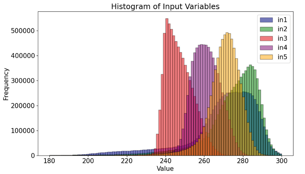
Figure 1: Data distribution for each continuous input variable in the dataset.
Figure 2: Data distribution for the target variable in the dataset.
A long-standing goal of Quantitative Precipitation Estimation has been to simulate radar data using radiometer data, with the Core Observatory providing coincident observations as a privileged source of radiometer-radar n-tuples. The aim is for the radiometers in the constellation to deliver radar-like precipitation estimates, significantly improving the temporal and spatial resolution of the constellation. Achieving this goal presents several challenges. Firstly, there are many contradictory cases in the datasets, where the same set of radiances yields different precipitation values. Secondly, the distribution is highly skewed, meaning traditional training methods would poorly represent high rainfall rates in the modeling. This results in outputs where high rainfall rates are treated as outliers, and the distribution is artificially driven towards a normalized probability density function (pdf)—an unrealistic representation that misrepresents the true nature of precipitation.
Regression algorithms
Regression is a fundamental technique in supervised machine learning used to predict continuous numerical values of a target variable. Unlike classification, which deals with categorical outputs, regression models aim to learn a mapping function from input variables (X) to continuous output variables (Y). This approach is widely applied across various domains to forecast trends, estimate unknown quantities, and understand relationships between variables.
To evaluate and compare the performance of different regression models, the following metrics were used:
R-squared (R2): measures the proportion of variance in the dependent variable explained by the model. Ranges from 0 to 1, with values closer to 1 indicating a better fit.
Root Mean Squared Error (RMSE): represents the average magnitude of the prediction errors. Lower values indicate better model performance, with greater sensitivity to larger errors.
Pearson Correlation Coefficient (PR): assesses the linear relationship between predicted and actual values, ranging from −1 (perfect negative) to 1 (perfect positive). Values closer to −1 or 1 represent a stronger linear association, where −1 indicates an inverse correlation and 1 indicates a direct correlation. A value near 0 suggests little to no linear relationship between the variables.
In the initial phase of this work, a pre-configured Python library was employed to automate the construction and evaluation of multiple regression models quickly (Pandala, 2022). This approach provided a broad overview of the performance of various algorithms without requiring manual implementation or fine-tuning. This initial exploration phase helped to identify the most promising models for the given dataset, focusing on baseline performance metrics while not yet considering the dataset’s inherent imbalance.
The results presented in Table 2 illustrate the performance of various pre-configured regression models applied to the dataset for the training period of April and the testing period of May. Upon examination of the top 10 models, it is observed that the RMSE values maintain relative stability, lacking significant enhancements. Consequently, the analysis will focus on R2 and PR metrics; the latter exhibits the greatest variance among the models. The Multi-layer Perceptron Regressor (MLPRegressor) achieved the highest R2 value of 0.63, indicating its effectiveness in capturing the underlying data patterns. This model’s superior performance can be attributed to its capability to learn complex nonlinear relationships among variables, which is essential when the data exhibits such complexities.
| Model | R2 | RMSE | PR | Time (s) |
|---|---|---|---|---|
| MLPRegressor | 0.63 | 0.54 | 0.795 | 460.49 |
| RandomForestRegressor | 0.62 | 0.55 | 0.787 | 462.15 |
| ExtraTreesRegressor | 0.61 | 0.56 | 0.783 | 82.66 |
| BaggingRegressor | 0.59 | 0.58 | 0.769 | 46.40 |
| LGBMRegressor | 0.58 | 0.58 | 0.766 | 1.17 |
| GradientBoostingRegressor | 0.58 | 0.58 | 0.765 | 72.96 |
| HistGradientBoostingRegressor | 0.58 | 0.58 | 0.762 | 1.83 |
| KNeighborsRegressor | 0.58 | 0.58 | 0.760 | 11.10 |
| XGBRegressor | 0.58 | 0.58 | 0.759 | 1.61 |
| ElasticNetCV | 0.32 | 0.74 | 0.566 | 3.19 |
| LassoCV | 0.32 | 0.74 | 0.566 | 2.85 |
| RidgeCV | 0.32 | 0.74 | 0.566 | 0.31 |
| BayesianRidge | 0.32 | 0.74 | 0.566 | 0.29 |
| Ridge | 0.32 | 0.74 | 0.566 | 0.20 |
| TransformedTargetRegressor | 0.32 | 0.74 | 0.566 | 0.20 |
| LinearRegression | 0.32 | 0.74 | 0.566 | 0.20 |
| OrthogonalMatchingPursuitCV | 0.32 | 0.74 | 0.566 | 0.63 |
| LassoLarsIC | 0.32 | 0.74 | 0.566 | 0.29 |
| LassoLarsCV | 0.32 | 0.74 | 0.566 | 0.78 |
| LarsCV | 0.32 | 0.74 | 0.566 | 0.69 |
| Lars | 0.32 | 0.74 | 0.566 | 0.18 |
| SGDRegressor | 0.32 | 0.74 | 0.566 | 0.86 |
| DecisionTreeRegressor | 0.30 | 0.75 | 0.642 | 6.20 |
| OrthogonalMatchingPursuit | 0.27 | 0.77 | 0.522 | 0.19 |
| TweedieRegressor | 0.26 | 0.77 | 0.530 | 0.27 |
| ExtraTreeRegressor | 0.26 | 0.77 | 0.644 | 0.94 |
In contrast, the Extra Trees Regressor demonstrated competitive R2 performance with a value of 0.61 while executing significantly faster than the MLP, with a time of only 82.66 s compared to the MLP’s 460.49 s but with a significant lower PR of 0.783 compared to 0.795 for the MLP. The Random Forest Regressor, although yielding a high R2 of 0.62, took even longer to execute at 462.15 s and also has a worse PR. This highlights a trade-off between execution time and predictive performance, as models like LGBM and XGB also yielded reasonable R2 scores of 0.58 while maintaining low execution times of 1.17 s and 1.61 s, respectively.
While this preliminary tool primarily facilitates the quick comparison of different models, it must be recognized that the default settings may not produce optimal performance. Therefore, the next phase focused on refining the 10 best performing models identified in Table 2. Using the scikit-learn library (scikit-learn developers, 2024), a systematic hyperparameter tuning process was implemented to improve the predictive accuracy of these selected models.
The results of the hyperparameter tuning are summarized in Table 3, which presents the performance metrics of the top 5 regression models after tuning.
| Top 5 models post tunning | R2 | PR |
|---|---|---|
| MLPRegressor | 0.64 | 0.80 |
| ExtraTreesRegressor and output | 0.63 | 0.80 |
| KNeighborsRegressor | 0.62 | 0.79 |
| BaggingRegressor | 0.62 | 0.79 |
| RandomForestRegressor | 0.62 | 0.79 |
The results presented in Table 3 indicate the improvements achieved through hyperparameter tuning for the top regression models. Notably, the Multilayer Perceptron Regressor (MLPRegressor) maintained its leading position, achieving a R2 value of 0.64, which demonstrates its ability to effectively model the underlying complexities of the data. Similarly, both the Extra Trees Regressor and Bagging Regressor showed a slight enhancement, confirming their effectiveness as ensemble methods that enhance predictive performance by reducing variance through the aggregation of predictions from multiple trees.
The KNeighborsRegressor, which was initially in the top 7 (see Table 2), also experienced an improvement in predictive accuracy, with its R2 value increasing from 0.58 to 0.62, claiming the top 3 spot, while also boasting the shortest execution time among the top models. This model’s performance can be attributed to its simplicity and the local nature of its predictions, which allows it to capture local patterns efficiently.
The five models that showed the best performances are detailed below:
MLPRegressor: a neural network-based approach that can capture complex non-linear relationships (Hornik, Stinchcombe & White, 1989).
KNeighborsRegressor: a method that predicts the value of a new observation by averaging the values of its nearest neighbors in the feature space (Altman, 1992).
ExtraTreesRegressor: an ensemble method that aggregates the predictions of multiple decision trees to improve accuracy and control overfitting (Geurts, Ernst & Wehenkel, 2006).
BaggingRegressor: ensemble technique that fits base regressors on random subsets of the original dataset and then aggregates their predictions (Breiman, 1996).
RandomForestRegressor: another ensemble learning method that constructs multiple decision trees during training and outputs the average prediction of individual trees for regression tasks. This technique enhances predictive accuracy and mitigates overfitting by leveraging the diversity of the ensemble (Breiman, 2001; Liaw & Wiener, 2002).
Among these, Multilayer Perceptron (MLPRegressor) was chosen as the reference model for further development, as it demonstrated slightly superior performance across the various evaluation metrics. This neural network model was preferred due to its flexibility in modeling complex patterns in data, making it particularly suitable for this regression task. Following the selection of the reference model, additional efforts were directed towards addressing the issue of data imbalance to further enhance its performance.
Facing data imbalance
The imbalance problem is evident, with a ratio of values where precipitation is greater than 0 compared to non-precipitation values of 1:8 (across all subsets). This imbalance is particularly distinctive because, in general, literature and other datasets often exhibit an imbalance with a range of values containing the majority of observations, as seen in Fig. 3. However, in this case, the value of 0, representing the absence of precipitation, is the only specific value that is overrepresented.
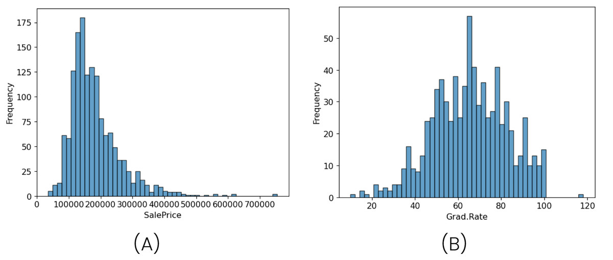
Figure 3: Illustration of frequency distributions using two different datasets.
The first image (A) represents the distribution of the SalePrice variable in housing data from California districts, summarizing key statistics based on U.S. census data. The second image (B) shows the distribution of the Grad.Rate variable from the College dataset, which includes data from 777 U.S. universities and colleges. Sources: College dataset from James et al. (2013); SalePrice dataset from Nugent (2020).
To address this, the first approach was to use different data preprocessing techniques (see Table 4). These include feature scaling and normalization, which, although they do not directly address the imbalance itself, play a crucial role in stabilizing the training process and ensuring numerical consistency across features.
| Preprocessing | R2 | PR |
|---|---|---|
| No preprocessing | 0.481 | 0.721 |
| Normalized inputs | 0.617 | 0.783 |
| Normalized inputs and output | 0.563 | 0.759 |
| Scaled inputs | 0.639 | 0.799 |
| Scaled inputs and output | 0.644 | 0.803 |
| Normalized inputs and output with log transformation on output | 0.704 | 0.840 |
| Scaled inputs and output with log transformation on output | 0.708 | 0.849 |
The results from Table 4 indicate that scaling and normalization applied to the input features significantly improve model performance, as demonstrated by the higher R2 and Pearson correlation values compared to the reference with no preprocessing.
Furthermore, after testing different transformation functions, the log1p logarithmic transformation, when applied together with input scaling, produced the best model performance. However, this improvement was only slightly better compared to using the same logarithmic transformation in conjunction with input normalization, achieving an R2 of 0.708 and a Pearson correlation of 0.849. This combination outperformed all other preprocessing techniques. The logarithmic transformation was particularly effective because it compresses larger values more than smaller ones, reducing the skewness and creating a distribution more conducive to learning. By mitigating extreme variations in the output variable, this transformation enables the model to better capture underlying patterns in the data.
These findings highlight the importance of selecting appropriate preprocessing techniques tailored to both the input and output variables. While input scaling alone provided a significant improvement, the introduction of a logarithmic transformation on the output further optimized the model’s predictive capacity. This was the optimal preprocessing configuration, and it will serve as the foundation for subsequent steps aimed at addressing data imbalance, including the application of under-sampling and over-sampling techniques.
Undersampling and oversampling
Based on the models described in Table 1, the following experiments implement and evaluate representative undersampling and oversampling techniques to address the specific imbalance characteristics of the dataset.
Initially, five classical and widely adopted oversampling techniques were evaluated: Random Oversampling (RO), SMOTE for Regression, Gaussian Noise Injection (GN), SMOGN, and KNNOR-Reg. These methods were selected for their relevance as foundational baselines in the literature (He & Garcia, 2009; Torgo et al., 2013; Menardi & Torelli, 2014; Branco, Torgo & Ribeiro, 2017; Belhaouari et al., 2025), as well as their availability in established open-source frameworks (Wu, Kunz & Branco, 2022). KNNOR-Reg, in particular, represents a more recent contribution that synthesizes samples through neighborhood-weighted aggregation and does not rely on a relevance function, in contrast to the other methods considered.
It is important to note that most of these methods rely on a relevance function to identify high-importance regions and guide the generation of synthetic samples. This dependency adds an extra layer of model complexity and tuning effort.
Figure 4 illustrates the density distribution after applying each method, and Table 5 summarizes the model performance. Contrary to expectations, all oversampling methods led to a consistent degradation in both R2 and Pearson correlation metrics. This is particularly significant given that these techniques represent the standard practice in the literature for addressing regression imbalance (Belhaouari et al., 2024).
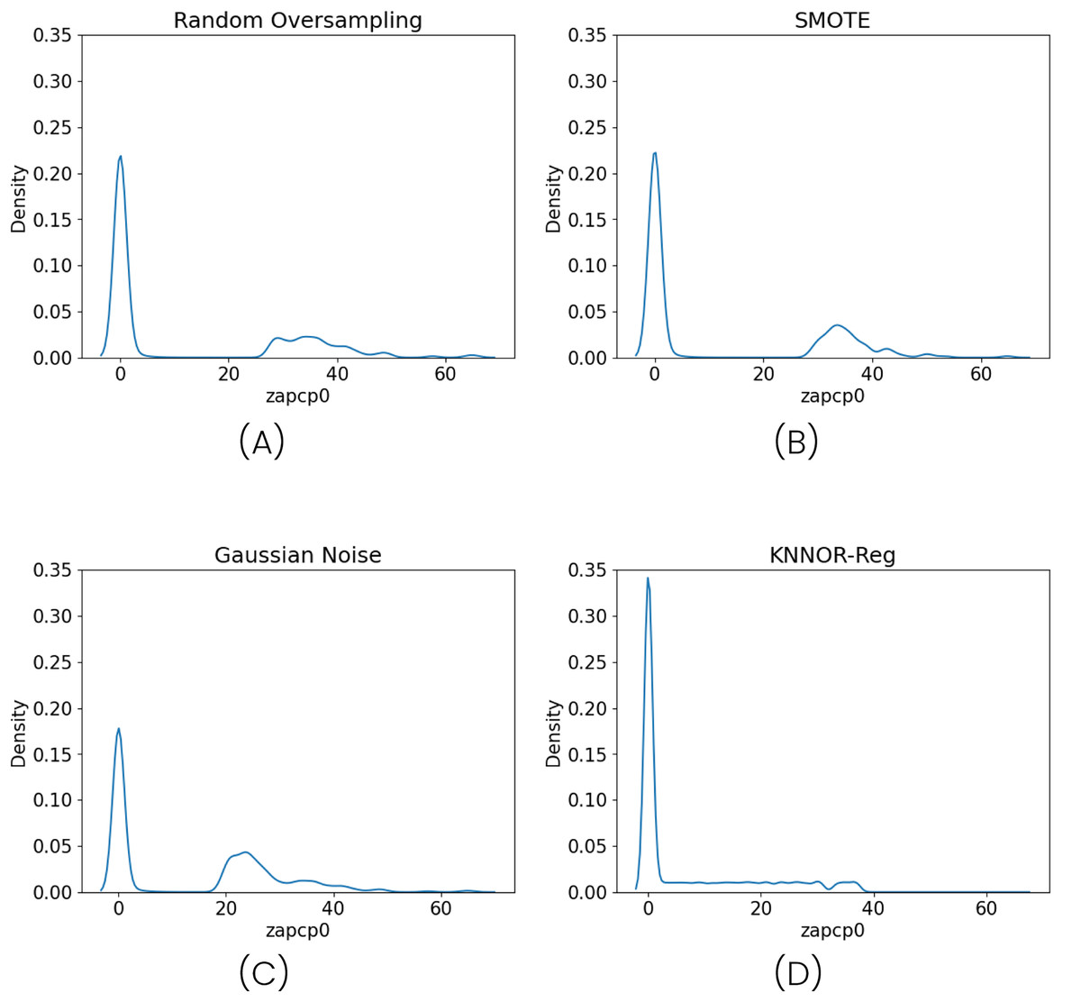
Figure 4: Density distributions after applying three different oversampling techniques: Random Oversampling (A), SMOTE (B), Gaussian Noise Oversampling (C) and KNNOR-Reg (D).
| Technique | R2 | Pearson |
|---|---|---|
| Without oversampling | 0.712 | 0.846 |
| KNNOR-Reg | 0.643 | 0.839 |
| Random oversampling | 0.623 | 0.817 |
| SMOGN | 0.564 | 0.812 |
| SMOTE | 0.587 | 0.809 |
| Gaussian noise | 0.501 | 0.800 |
These results suggest that oversampling techniques may not be suitable in this case. The generation of synthetic samples can introduce noise or artificial structures that distort the original distribution, particularly when high-density areas (e.g., zero-precipitation regions) dominate the dataset. Neural networks are especially sensitive to such distortions, which may alter the optimization landscape and exacerbate overfitting. The fact that even SMOGN—one of the most refined oversampling techniques—underperforms in this context reinforces the idea that oversampling is not a reliable solution for this type of structured imbalance.
On the other hand, undersampling is often seen as a natural complement to oversampling, particularly for mitigating the dominance of majority values. However, eliminating values without considering the structure of the dataset may break continuity or remove relevant transitional states. This is especially true in our dataset, where the dominant value (zero) appears in long, consecutive sequences.
While techniques such as ENN, Tomek Links, and CNN have been considered, they are typically designed to remove boundary noise or misclassified instances in classification tasks, and are not directly applicable when a single target value overwhelmingly accounts for the imbalance. In this case, regardless of the strategy used, the goal of any undersampling method becomes the selective reduction of the zero value—raising the need for structure-aware solutions.
Sequence-based undersampling (SBU)
The SBU is designed to address imbalance in datasets with sequentially ordered observations by effectively removing a specific ratio of over-represented values in consecutive sequences (see Algorithm 1). This approach is particularly useful when data is labeled with a timestamp or an implicit index that reflects the recording order, and exhibits significant numbers of repeated values in prolonged streaks.
| 1: Input: Dataset D, target column C, target value v, ratio to remove r |
| 2: Output: Filtered dataset Dnew |
| 3: Initialize a list of consecutive sequences L |
| 4: Initialize a counter |
| 5: Initialize an empty list Iremove for indexes to remove |
| 6: Extract the target column C from the dataset D |
| 7: for each i, x in C do ▹ i is the index and x=C[i] |
| 8: if then |
| 9: Increment count |
| 10: else |
| 11: if then |
| 12: Append the sequence (i – count, count) to L |
| 13: Reset |
| 14: end if |
| 15: end if |
| 16: end for |
| 17: if then |
| 18: Append the last sequence (length(C) – count, count) to L |
| 19: end if |
| 20: if L is not empty then |
| 21: Compute the average length of sequences |
| 22: else |
| 23: Return the original dataset D |
| 24: end if |
| 25: for each sequence (start, length) in L do |
| 26: if then |
| 27: Calculate the number of elements to remove: |
| 28: Add the corresponding indices to Iremove |
| 29: end if |
| 30: end for |
| 31: Create a mask for the dataset D that includes all elements |
| 32: Set the mask to exclude indices in Iremove |
| 33: return the filtered dataset Dnew |
Note:
This algorithm is implemented specifically for the value of 0; however, it can be generalized to manage multiple consecutively overrepresented values in a temporally ordered dataset.
The algorithm works as follows: it iterates through the target column, identifying consecutive sequences of a specified value (e.g., zero). These sequences are recorded with their start index and length. Once all sequences are identified, the average sequence length is computed. Sequences longer than this threshold are considered redundant and selected for undersampling. A fixed ratio of values within these longer sequences are randomly removed. This ensures that only excessively long streaks are reduced, while shorter, potentially informative sequences are preserved. A boolean mask is finally created to filter out the selected indexes, resulting in a new dataset with the over-represented values reduced while preserving the natural order in which the data was recorded.
The algorithm is governed by a single parameter: the removal ratio , which determines the proportion of values to eliminate within the identified long sequences. To select a robust value for , a sensitivity analysis was conducted for each data subset, evaluating values from 0.0 to 0.8. The optimal performance was consistently observed when ranged between 0.4 and 0.6. Based on this observation, a fixed value of was used throughout the experiments. Variations within this range yielded changes of less than 2–3% in performance metrics, confirming the method’s robustness to this parameter.
This algorithm operates under two essential conditions: first, the dataset must include either a temporal label or any consistent indexing that reflects the order in which the data points were recorded; second, the dataset must be sorted according to this order. This ensures that the method can accurately identify and process consecutive sequences of repeated values, preserving the natural recording structure while addressing overrepresented targets.
After the detailed steps of the SBU algorithm, it is essential to assess its computational complexity to understand its efficiency and scalability. The algorithm processes the dataset in linear time, with a complexity of to identify consecutive sequences in the target column, where is the total number of samples. Subsequent operations, including calculating the average sequence length and undersampling longer sequences, depend on the number of identified sequences . Since is typically much smaller than , the overall time complexity remains . Memory requirements are dominated by the storage of sequence indices and the filtering mask, resulting in a space complexity of .
Comparison with other undersampling methods
A range of established undersampling techniques were considered for comparative evaluation, including Edited Nearest Neighbors (ENN), Condensed Nearest Neighbor (CNN), and Tomek Links. These algorithms were implemented using the same Python library employed for the oversampling experiments (Wu, Kunz & Branco, 2022). However, during execution, ENN, CNN, and Tomek resulted in memory allocation errors or prohibitively long processing times. This behavior stems from their reliance on constructing and evaluating pairwise distance matrices of size up to , where in our dataset. For these reasons, these neighborhood-based methods were excluded from the final evaluation due to memory failures and excessive computational demands.
Selective Under-Sampling (SUS) also relies on a neighborhood-based approach, aiming to reduce the number of low-relevance instances while preserving those that are either isolated or representative of locally homogeneous regions in the input space. However, in scenarios where the imbalance arises from the overwhelming concentration of a single target value—such as precipitation measurements equal to zero—the relevance function assigns the same minimum score to all such instances. As shown in Table 6, the performance of SUS was inferior to that of the proposed SBU algorithm ( , PR = 0.842), and only marginally better than the lower bound observed for RU.
| Technique | R2 | Pearson |
|---|---|---|
| SBU | 0.728 | 0.858 |
| WERCS (only undersampling) | 0.713 | 0.850 |
| RU | (0.491–0.702) | (0.667–0.834) |
| SUS | 0.705 | 0.842 |
Note:
RU was executed multiple times due to its stochastic nature, and the R2 and Pearson results are reported as intervals reflecting the minimum and maximum values observed across runs.
In addition, the WERCS method (Branco, Torgo & Ribeiro, 2019) was evaluated using only its undersampling component. Although WERCS is inherently a hybrid technique that combines oversampling and undersampling based on a relevance function, only the elimination mechanism was activated. This decision was motivated by previous results (see Table 5), which showed that the generation of synthetic data consistently degrades model performance. The WERCS elimination mechanism probabilistically discards instances according to their relevance scores: values with low relevance—such as zeros in our case—are more likely to be removed. This behavior mimics random undersampling, but introduces a relevance-weighted bias in the selection. As observed in Table 6, the performance of WERCS ( , PR = 0.850) was superior to that of both RU and SUS, although it did not surpass the performance of the proposed SBU method.
Overall, the results support the assertion that existing undersampling methods exhibit limitations in scenarios where imbalance is caused by a dominant value with high temporal redundancy. The Sequence-Based Undersampling (SBU) algorithm addresses this limitation by leveraging the sequential structure of the data to selectively reduce such redundancy while preserving the integrity of the temporal sequences. This advantage is reflected in its superior performance ( , PR = 0.858), as shown in Table 6.
Results
The training and testing procedure is aimed to mimicry meteorological operations in the QPE field. Thus, we train with 1 month worth of radiometer-radar data and use the trained net to estimate the precipitation in the following month using the radiometers only. Apart from the operational point of view, sequential months present better training performances that using the full dataset, randomly selected months, or even the same month in the previous years, which induces an unwanted climatological bias into the training.
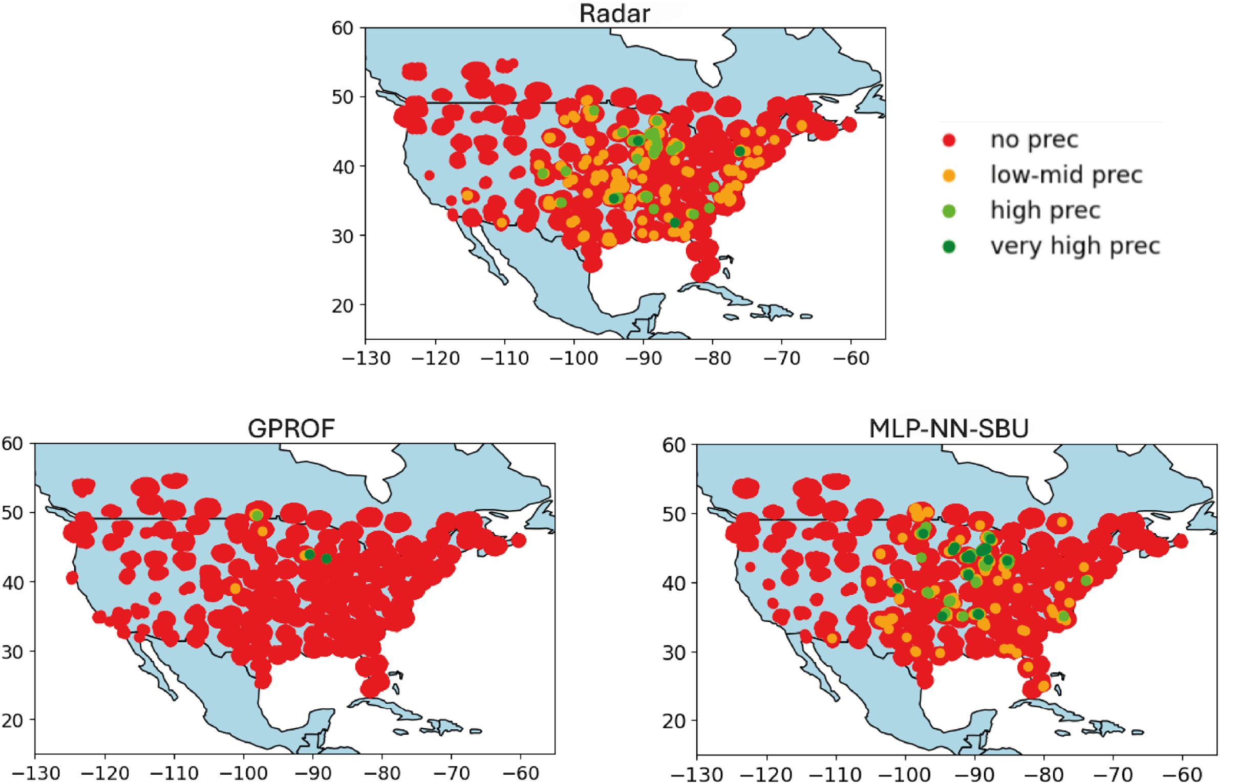
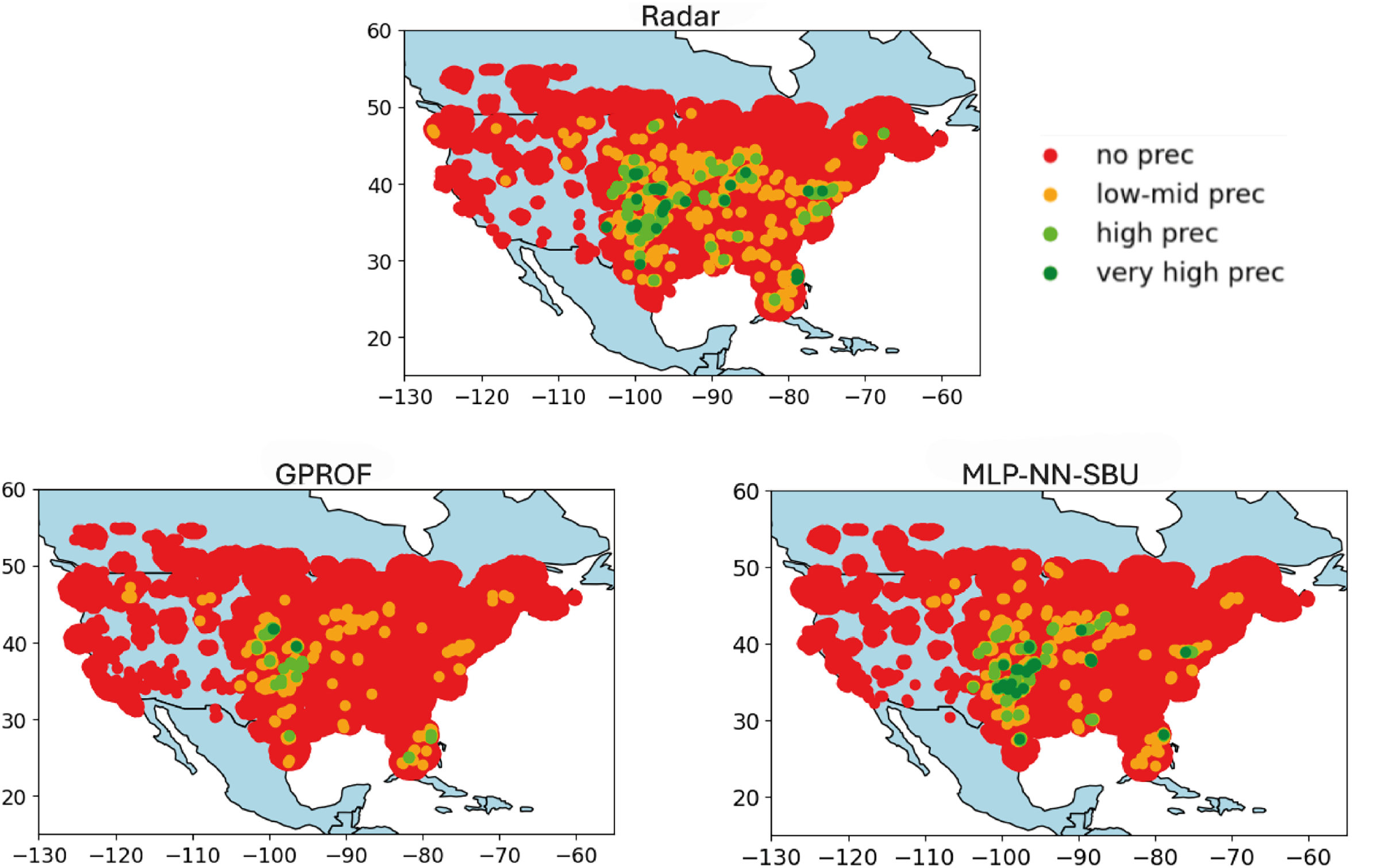
The results in Fig. 7 shows the worst-case scenario; Fig. 6 the average case, and Fig. 5 the best case.
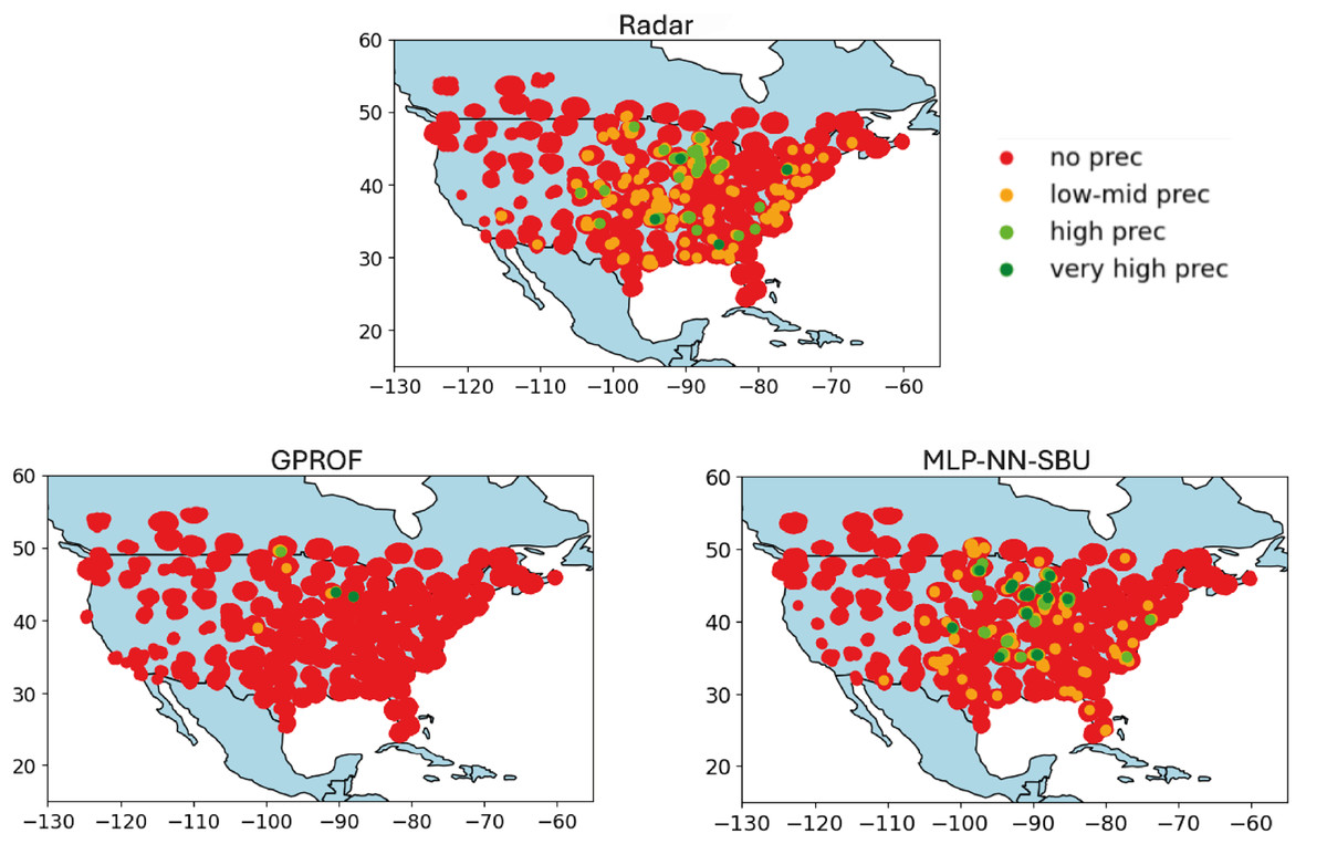
Figure 5: Heatmap comparison (best case): real value “Radar”, baseline Model “GPROF”, and the MLP-NN SBU model utilizing data from July 2018 to august 2018.
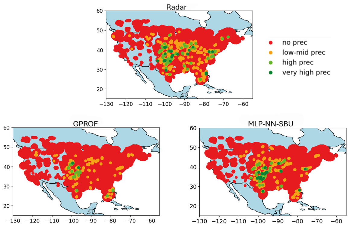
Figure 6: Heatmap comparison (average case): real value “Radar”, baseline model “GPROF”, and the MLP-NN SBU model utilizing data from april 2018 to may 2018.
Figure 7: Heatmap comparison (worst case): real value “Radar”, baseline model “GPROF”, and the MLP-NN SBU model utilizing data from March 2018 to April 2018.
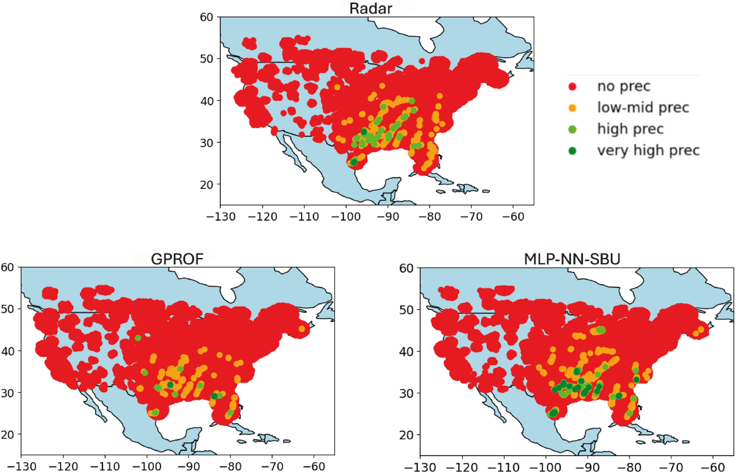
No Precipitation: data points with values below the first quartile (Q1) are colored red, indicating minimal or no precipitation.
Low to Medium Precipitation: data points between Q1 and the median (Q2) are colored orange, depicting lower precipitation levels.
High Precipitation: data points between the median (Q2) and the third quartile (Q3) are colored lime, representing higher precipitation levels.
Very High Precipitation: data points above the third quartile (Q3) are colored green, indicating intense precipitation.
The heatmaps compare the output, labeled as “Radar” (nominal truth), with the model estimates, referred to as “NN-MLP SBU” and a reference model output, “GPROF” (Olson et al., 2007). The purpose of the heatmaps is to visually represent the spatial correspondence between the model’s estimates and the observed values, a feature that is important but hidden in a scatterplot. The heatmaps are built as follows:
Variable Data Binning: the data is divided into quartiles. Quartiles are statistical measures that divide the data into four equal parts, providing a more clear depiction of its distribution. The median and quartiles (Q1, Q2, and Q3) are calculated to establish thresholds for categorizing the data. These quartiles define meaningful thresholds to classify the data into different intensity levels, ranging from no precipitation to high precipitation.
Color Coding and Visualization: data points are color-coded based on these quartile thresholds:
This color coding allows for a more intuitive visual assessment of how different levels of precipitation are distributed in the Conterminous (Continental) United States (CONUS). Indeed, the actual data is greatly imbalanced and difficult to plot using a linear or logarithmic scale.
Figure 5 illustrates the best-case scenario in terms of neural networks (NNs) outperforming an alternative algorithm. It is clear that the MLP-NN model compares best with observations.
In contrast, Fig. 6 represents a standard scenario. Although the Multi-Layer Perceptron (MLP) NN with SBU is capable of recognizing rainfall patterns, its predictive accuracy diminishes when faced with moderate precipitation levels. This suggests that the model faces challenges in generalizing its predictions across varying intensity levels of rainfall.
Finally, Fig. 7 depicts the worst-case scenario, where precipitation is concentrated in specific areas of the map. While the model can identify the rain-affected regions, it tends to overestimate the intensity of the rainfall. This discrepancy underscores a consistent challenge in accurately predicting extreme rainfall rates. Indeed, the detection of extremes remains a challenging task for the NN-MLP, SBU model in some cases even with a sequence-based undersampling algorithm. Overall, however, the performances present some moderate improvement over other approaches.
Conclusions
Data imbalance is a critical challenge for ML algorithms, particularly in QPE, as precipitation is a highly skewed variable. Indeed, the pdf of precipitation at any temporal aggregation presents a significant skew, with light rainfall rates dominating over higher values. The leptokurtic character of the distribution presents a formidable challenge for regression using NN-MLPs, often resulting in a regression to the mean that misrepresents the true structure of the variable and its spatial distribution.
This study explored multiple data preprocessing methods to mitigate the bias introduced by imbalanced data. While oversampling strategies are commonly used to balance datasets, they did not provide significant improvements in this case. Thus for instance, duplicating infrequent events did not enhance the model’s generalization capacity.
Undersampling proved to be a more effective strategy. Baseline methods in the literature such as ENN, Tomek Links, CNN, WERCS and SUS, although useful in other settings, were not suitable here due to the nature of the imbalance. Therefore, RU emerged as an initial solution to address the overrepresentation. However, because of its stochastic nature, it exhibited high variability in performance. In contrast, both SUS and WERCS provided more stable and consistent results, and WERCS achieved the best performance among existing methods. Nonetheless, neither surpassed the SBU algorithm, which consistently outperformed all other approaches in evaluation metrics.
The key contribution of this work is the development of the Sequence-Based Undersampling (SBU) algorithm, which leverages the temporal order of data to selectively reduce overrepresented values. This method not only balances the dataset but also preserves essential temporal relationships, leading to improvements in R2 and Pearson correlation metrics. Additionally, the reduction in dataset size resulted in more efficient model execution times. The applicability of the SBU is not limited to precipitation retrievals but to any other types of highly-skewed continuous data. However, its effectiveness depends on the ability to clearly identify overrepresented values and the presence of consecutive sequences of these values, as observed in this study with precipitation measurements dominated by excessive sequences of zeros.
Despite the advance represented by the application of SBU techniques to NN-MLP modeling, challenges in QPE remain. While in general the method over-performs alternative algorithms, the model continues to struggle with accurately predicting medium to high precipitation in certain regions and cases. Future work could explore anomaly detection techniques to further improve model performance in these complex cases.
Supplemental Information
Code of SBU algorithm.
Python implementation of the proposed SBU undersampling algorithm applied to eliminate non-precipitation.
Basic statistical data analysis.
Number of data per month, number of zero and non zero values, mean, etc.
2018 Results of the SBU undersampling technique.
Results of the SBU undersampling technique with different % of undersampling.
2019 Results of the SBU undersampling technique.
Results of the SBU undersampling technique with different % of undersampling.