
Combining convolutional neural network with transformer to improve YOLOv7 for gas plume detection and segmentation in multibeam water column images
- Published
- Accepted
- Received
- Academic Editor
- Siddhartha Bhattacharyya
- Subject Areas
- Algorithms and Analysis of Algorithms, Computer Vision, Data Mining and Machine Learning, Optimization Theory and Computation, Neural Networks
- Keywords
- Multibeam water column image, Gas plume, Target detection and segmentation, YOLOv7, Transformer, Bi-level routing attention
- Copyright
- © 2025 Chen et al.
- Licence
- This is an open access article distributed under the terms of the Creative Commons Attribution License, which permits using, remixing, and building upon the work non-commercially, as long as it is properly attributed. For attribution, the original author(s), title, publication source (PeerJ Computer Science) and either DOI or URL of the article must be cited.
- Cite this article
- 2025. Combining convolutional neural network with transformer to improve YOLOv7 for gas plume detection and segmentation in multibeam water column images. PeerJ Computer Science 11:e2923 https://doi.org/10.7717/peerj-cs.2923
Abstract
Multibeam bathymetry has become an effective underwater target detection method by using echo signals to generate a high-resolution water column image (WCI). However, the gas plume in the image is often affected by the seafloor environment and exhibits sparse texture and changing motion, making traditional detection and segmentation methods more time-consuming and labor-intensive. The emergence of convolutional neural networks (CNNs) alleviates this problem, but the local feature extraction of the convolutional operations, while capturing detailed information well, cannot adapt to the elongated morphology of the gas plume target, limiting the improvement of the detection and segmentation accuracy. Inspired by the transformer’s ability to achieve global modeling through self-attention, we combine CNN with the transformer to improve the existing YOLOv7 (You Only Look Once version 7) model. First, we sequentially reduce the ELAN (Efficient Layer Aggregation Networks) structure in the backbone network and verify that using the enhanced feature extraction module only in the deep network is more effective in recognising the gas plume targets. Then, the C-BiFormer module is proposed, which can achieve effective collaboration between local feature extraction and global semantic modeling while reducing computing resources, and enhance the multi-scale feature extraction capability of the model. Finally, two different depths of networks are designed by stacking C-BiFormer modules with different numbers of layers. This improves the receptive field so that the model’s detection and segmentation accuracy achieve different levels of improvement. Experimental results show that the improved model is smaller in size and more accurate compared to the baseline.
Introduction
Underwater acoustic imaging technology uses the principle of acoustic wave propagation in water to image and detect underwater targets (Ferreira et al., 2016), which has a wide range of applications in the fields of ocean engineering (Hansen, 2013), marine resource exploration (Meng, Yan & Zhao, 2022), and underwater target monitoring (Mignotte et al., 2000). Multibeam echo sounding, as an important underwater acoustic detection technique, employs a combination of multiple sonar beams to acquire detailed water body data and generate high-resolution water column image (WCI). This technology significantly enhances the accuracy of underwater target detection and recognition (Colbo et al., 2014; Li et al., 2023b). Moreover, the segmentation task for underwater targets can provide more accurate target boundary information, which makes the results of target detection more reliable. Natural gas, as a non-renewable energy source, is becoming increasingly scarce on land, while underwater gas plumes often indicate the presence of significant natural gas within nearby sediment layers (Römer et al., 2019; Zhang et al., 2021). Therefore, how to accurately detect and segment the gas plume in multibeam WCI has become an important research topic.
Underwater gas plumes exhibit low backscatter intensity, often moving in the direction and speed of water currents during the upflow process, which can lead to fragmentation. These plumes, characterized by elongated forms composed of numerous bubbles, lack distinct outline information in WCI, posing significant challenges for the detection and segmentation of gas plume targets. Traditional identification methods primarily rely on manually designed features and rules for target matching, e.g., Urban, Köser & Greinert (2016) used data within the minimum slant range (MSR) and by setting appropriate thresholds divided pixels in the image into regions containing gas plume targets and other marine feature areas. Schimel, Brown & Ierodiaconou (2020) divided the image into two parts at the MSR and set different thresholds according to the changes of backscatter intensity in each region to retain the target information. To reduce the noise interference in the image, Ren et al. (2022b) subtracted the original image from its symmetric image, reduced the environmental noise, and then extracted the gas plume target in the image by density clustering. In Hou & Huff (2004), the water body data were normalized to reduce the interference of sidelobe noise. In the use of machine learning methods, Huo et al. (2017) used k-means to coarsely segment the image pixels, and then used the region fitting method to keep the target boundary continuous, which effectively achieved the target segmentation. In Cui et al. (2021), the geometric features were extracted from the multibeam bathymetry data and fed them into the support vector machine (SVM) classifier for training, which realized the automatic classification of underwater targets. Traditional threshold segmentation and edge detection methods both require setting parameters and cannot fully capture and express the complex shapes of gas plume targets. Machine learning methods require manual design of features, which need a lot of prior knowledge and experimental verification, and the steps are complicated. In addition, traditional methods make it difficult to extract high-level semantic information, which poses a great limitation for identifying gas plume targets that have complex shapes or are similar to the background.
To improve the traditional target detection and segmentation effects, researchers introduced a series of target detection and semantic segmentation algorithms based on convolutional neural network (CNN). CNN extracts feature by applying a series of convolutional layers and pooling layers on the image. Convolutional layers use convolutional kernels to extract local features in the image. Pooling layers are used to reduce the spatial size of the feature map while retaining important information and reducing the amount of computation. In the field of target detection, the most representative network structures are the region-based CNN (R-CNN) series and the YOLO (You Only Look Once) series. R-CNN (Girshick et al., 2014) is the pioneer of target detection, it introduces the concept of region proposal and identifies regions that may contain targets by using the selective search algorithm, then uses CNN to classify each region. Fast R-CNN (Girshick, 2015) introduces an region of interest (ROI) pooling layer, which improves the speed and accuracy of R-CNN. Faster R-CNN (Ren et al., 2017) introduces the Region Proposal Network (RPN), which is used to generate candidate regions, and further accelerates the process of target detection. In Sun et al. (2025), the authors replaced the Softmax classifier in Faster R-CNN with a random vector to address the problem of low detection accuracy in the case of scarce data. In Ke et al. (2021), deformable convolution was used to replace standard convolution, allowing the improved Faster R-CNN to better adapt to targets with different angles. The YOLO series (Wang, Yeh & Liao, 2024; Tian, Ye & Doermann, 2025) abandons the region proposal and directly predicts the bounding box and class probability of the target on the whole image, thus having a faster detection speed and balancing the contradiction between model speed and accuracy. In applications, Wang et al. (2023) added coordinate attention to the YOLOv5 model, which improved the model’s relative relationship between target locations, allowing it to better capture key features. To improve the accuracy of small object detection, Zhao, Zhang & Zhao (2023) added a small object detection head to YOLOv7 and combined it with data augmentation strategy, resulting in a significant improvement in detection results. In the field of semantic segmentation, the model learns the semantic information of each pixel in the image, and classifies it according to its semantic category, thus achieving pixel-level accurate segmentation. The earliest CNN used for semantic segmentation is fully convolutional network (FCN) (Long, Shelhamer & Darrell, 2015), which uses transposed convolution for upsampling, making it suitable for pixel-level prediction. U-Net (Ronneberger, Fischer & Brox, 2015) adopts an encoder-decoder structure and introduces skip connection operation, which allows it to learn more detailed information. DeepLab (Chen et al., 2018) introduces techniques such as dilated convolution and spatial pyramid pooling, which enhance the network’s perception ability for large-scale targets. High-Resolution Net (HRNet) (Sun et al., 2019) improves the segmentation performance by fusing high-resolution and low-resolution features. Mask R-CNN (He et al., 2017) uses a shared CNN to extract features, and adds a target detection branch and a semantic segmentation branch, allowing it to simultaneously locate and segment targets. In applications, to reduce the interference of noise echoes such as suspended matter in sonar images, Zheng et al. (2021) designed a symmetric information synthesis module to weaken the noise echoes and added it to DeepLabv3+ to improve the segmentation ability of the model. In Yi et al. (2024), based on Mask R-CNN, the authors utilized coordinate convolution and group normalization methods to improve the model’s attention to underwater targets. In Xu et al. (2022), the label consistency between each pixel and its neighbors was calculated, which made the prediction results more consistent in local regions and reduced the discontinuity in segmentation. Compared to classification tasks, semantic segmentation provides more detailed and accurate image understanding by more accurately labeling the semantic information of each pixel in an image, enabling pixel-level classification and localization.
CNN has been dominating the computer vision field for the past time, but it still has some drawbacks. In feature extraction, CNN uses a fixed-size convolutional kernel, the size of the receptive field is limited by the structure of the network, which cannot effectively capture long-distance dependencies in the image, and the translation invariance of the convolutional operation makes the network not well adapted to face some shape-shifting targets, limiting the performance of the model. Also, the appearance of the transformer solves this problem well. Based on the self-attention mechanism, it can take into account the information of other positions while processing the current position, which makes up for the deficiency of CNN in dealing with long-distance relationships (Vaswani et al., 2017). The self-attention mechanism can assign different attention weights to pixels at different positions according to the change of target position, which makes the transformer more adaptable to feature extraction of deformed targets. Liu et al. (2024) utilized the window self-attention in Swin Transformer to establish global relationships and enhance the extraction of global features of underwater targets. Wang et al. (2024) constructed lightweight modules through reparameterization to reduce the model complexity of Vision Transformer and improve the model efficiency. Verma & Puthumanaillam (2023) segmented the water body regions in remote sensing images by fusing the features of UNet and Vision Transformer, but there is still room for improvement in the edge and small target parts. Therefore, in this article, the transformer module is added to the CNN, fusing the advantages between the two to make the network have better detection and segmentation. The main contributions are as follows:
The experimental results show that the enhanced feature extraction module is more suitable for the underwater morphology of the gas plume target only in the deep network of the backbone network.
The C-BiFormer module is proposed, and its sparsity reduces the number of parameters, computation and memory consumption of the network, and realizes the effective cooperation between local feature extraction and global semantic modeling.
Based on the C-BiFormer module, two kinds of network models of different sizes are constructed, and the network can adapt to different hardware resources and accuracy requirements under the premise of improving accuracy.
Numerous comparison and ablation experiments have been conducted for the improved module, verifying that the proposed model exhibits better results overall and enables more accurate detection and segmentation in the testing of multibeam WCI.
Related work
Segmentation model for YOLOv7
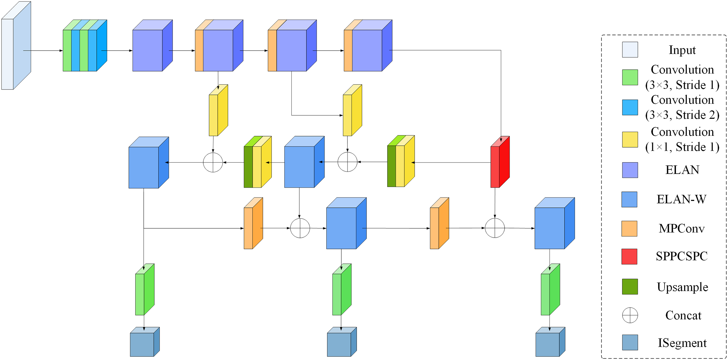
As an advanced target detection network model, YOLOv7 (Wang, Bochkovskiy & Liao, 2023) has shown higher detection accuracy and speed under various tricks, and has achieved good results in posture estimation (Yang, Zhang & Liu, 2022), target tracking (Le, 2022), and semantic segmentation (Yasir et al., 2023). The segmentation model of YOLOv7 is similar to the detection model. The model structure, compared with the previous models of the YOLO series, mainly adds the Efficient Layer Aggregation Network (ELAN) (Wang, Liao & Yeh, 2022), ELAN-W, MPConv and the Spatial Pyramid Pooling and Cross-Stage Partial Connection (SPPCSPC) (Wang et al., 2020) modules (As shown in Fig. 1). Unlike YOLOv7’s detection model, YOLOv7’s segmentation model uses YOLOR’s segmentation head (Wang, Yeh & Liao, 2021), which can simultaneously detect and segment targets, allowing recognition and segmentation tasks to share parameters and enhance feature representation.
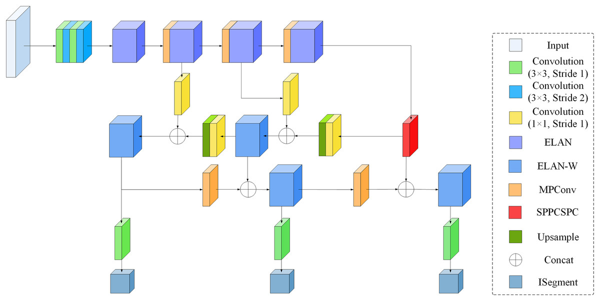
Figure 1: Segmentation model structure of YOLOv7.
Transformer-based self-attention mechanism
Transformer is a sequence-to-sequence model based on a self-attention mechanism (Vaswani et al., 2017), consisting of an encoder and a decoder. Both the encoder and decoder consist of several layers, and each layer contains two sublayers, the multihead self-attention (MSA) and the multi-layer perceptron (MLP). As shown in Fig. 2A, each sublayer has a residual connection and a layer normalisation (LN) to accelerate convergence and optimize network parameters. MSA is an attention mechanism that allows the model to simultaneously attend to information from different locations in different representation subspaces. It obtains the query (Q), key (K), and value (V) matrices by linearly transforming the feature map. The Q and K matrices are used to compute the weights when computing the attention weights and the obtained weights are applied to the V matrix, which results in weighted assignment and integration of information. Specifically, for each header h, we can compute its output weight result as:
(1) where denotes the dimension of the K matrix, which is used to scale the similarity and keep the training stable. The outputs from all the heads are then stitched together and linearly transformed to allow the model to capture multiple relationships and features. The formula is:
(2) where is the total number of heads and is the linearly transformed weight matrix used to fuse the attention outputs of multiple heads. MSA provides more flexibility as it can learn different relationships in different representation subspaces, which is useful in many tasks such as machine translation (Lee et al., 2014), text summarisation (Hoang et al., 2019), and speech recognition (Dong, Xu & Xu, 2018). However, with the development of deep learning techniques, the transformer is also widely used in computer vision. DETR (DEtection TRansformer) (Carion et al., 2020), as the first model to apply the transformer to target detection, uses a transformer encoder to transform the input image into a sequence of feature vectors and then uses a transformer decoder to generate bounding box and category predictions. The advantages of DETR over traditional region extraction-based target detection methods (Jocher et al., 2022; Ren et al., 2017) are that it can better handle different sizes and numbers of targets and can directly predict the whole image. Besides DETR, Vision Transformer (ViT) (Dosovitskiy et al., 2020) and Swin transformer (Liu et al., 2021b) are typical models for applying transformer in vision tasks. Compared to the standard transformer module, ViT achieves no weaker results than CNN by generating embedded patches (Fig. 2B) only during the input process. After the image is segmented into a set of small image patches, each image patch is flattened into a vector, and the vector is transformed into a fixed-dimension vector representation through a fully connected layer, which is used as input to the transformer model. To introduce the position information in the image patch, each vector representation will also embed a position encoding. To support the classification task, ViT also introduces a special classification token as the first input of the sequence, which represents the category information of the whole image. After these preprocessing operations are completed, the vector representations of the image patches will be fed into a transformer encoder. Each vector representation will undergo processing and interact with other vectors to generate a final output vector, which is used for image classification. Therefore, the partitioning of the image into patches enables ViT to better learn spatial structural information within the image and capture the dependencies among image patches. Figure 2C displays the basic module of the Swin transformer model, where the windowed multihead self-attention (W-MSA) and shifted windowed multihead self-attention (SW-MSA) are two attention mechanisms used in the Swin transformer to replace the traditional MSA. In W-MSA, the input feature map is divided into several non-overlapping windows, and multihead self-attention computation occurs among tokens within each window. This approach reduces computational complexity, particularly when dealing with large shallow-level feature maps. However, due to the independence among different windows, W-MSA is unable to capture information across different windows. To solve this problem, Swin transformer introduces SW-MSA, which first shifts the input feature maps and then performs window partitioning and multihead self-attention computation to achieve the effect of transferring information between neighboring windows. In addition, the Swin transformer also introduces the patch merging operation between these base modules to reduce computational complexity and achieve lossless downsampling of feature map information. To reduce the training difficulty, this article also uses the Transformer module with low complexity for global information extraction, but global self-attention tends to reduce the model’s sensitivity to local details, and due to the complex underwater environment, slight fluctuations can affect the shape and size of the bubble flow, generating some of the small targets, which leads to a reduction in its detection performance for small targets. In this article, we use this as a starting point for module and model improvement to enhance the model’s ability to extract multi-scale targets.
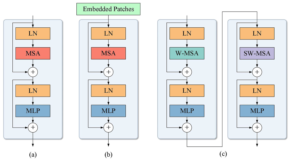
Figure 2: Structure of different transformer modules.
(A) Transformer base module. (B) ViT base module. (C) Swin transformer base module.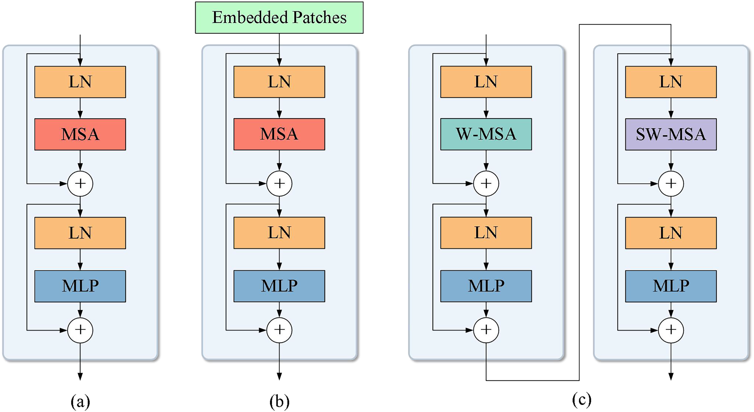
Method
Bi-level routing attention in the BiFormer model
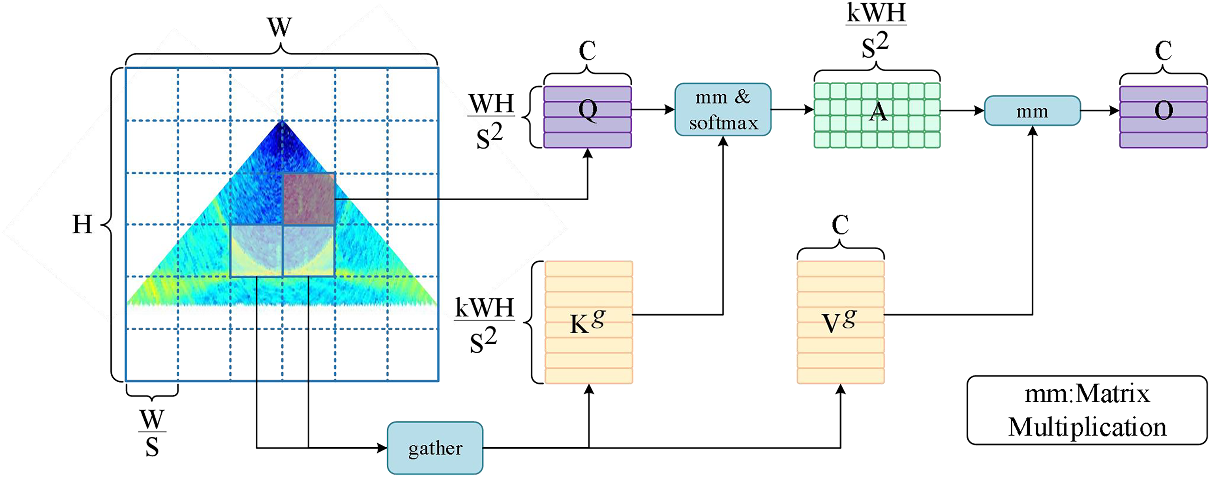
The transformer model is capable of capturing dependencies over long distances and has the advantage of global modeling. However, it requires the use of self-attention to calculate the similarity between each location and other locations to determine the corresponding attention weights. The computation grows exponentially as the length of the input sequence increases. Meanwhile, the transformer model has a large number of parameters distributed in the embedding layer, the MSA layer, and the MLP layer, so the model requires a large amount of GPU memory to store the intermediate results and compute the gradients during training. To address this problem, researchers have begun to explore the use of methods such as local windows (Zhou et al., 2021; Parmar et al., 2018) or sparse attention (Child et al., 2019; Ren et al., 2021) to reduce the number of parameters, computation, and memory requirements. Bi-level routing attention in BiFormer is a dynamic, query-aware sparse attention (Zhu et al., 2023), the main idea of which is to divide the input image sequence into different regions and perform coarse-grained filtering to exclude the regions that are not relevant to the target, and then to perform fine-grained token-to-token attention in the retained important routing regions. The schematic diagram of the module is shown in Fig. 3, and the specific implementation is as follows. Step 1: Region partition and input projection.
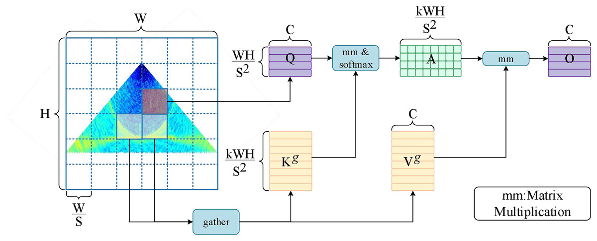
Figure 3: Schematic diagram of bi-level routing attention.
The input feature map is first divided into non-overlapping regions, each containing feature vectors, so that the feature map can be adapted to . Then the query, key, and value tensor is obtained using a linear transformation: , , , , , , where , , are the learnable weight matrices corresponding to query, key, and value. Step 2: Region-to-region routing with a directed graph. The region-level query and key: , are first obtained by averaging the features of each region and applying them to the computation of Q and K, respectively. The affinity graph adjacency matrix between the regions is then derived by matrix multiplication between the and transpositions. The adjacency matrix represents the degree of semantic association between the two regions. Finally, the affinity graph is pruned by retaining the first k connections of each region through the routing index matrix : , , where the ith row of denotes the k most relevant region indexes to the ith region. Final step: Token-to-token attention. After obtaining the top k relevant regions for each region through , fine-grained operations can be performed. For each region, the key and value tensor corresponding to the related regions can be gathered and expressed as follows: , , , . The gathered key-value pairs are then used to capture distant dependencies using the self-attention operation:
(3)
refers to deep convolution over tensor V for enhanced localization (Ren et al., 2022a). BiFormer introduces a bi-level routing attention mechanism that enables the model to selectively attend to key-value pairs relevant to the query in a content-aware manner. This dynamic allocation of attention not only improves computational performance and efficiency and reduces memory consumption, but also enables the model to have higher representation capability and generalization performance.
C-BiFormer module and model structure
Considering the powerful global modeling capability of the transformer and the local feature extraction capability of CNN, this article designs the C-BiFormer module as the basic module in the improved model. Specifically, the C-BiFormer module uses sequential concatenation. First, it extracts local features using convolution, and then expands the contextual associations of these local features to the global scale through the BiFormer, forming a progressive feature enhancement from local perception to global modeling. The structure is shown on the right side of Fig. 4. Firstly the convolutional layer uses a set of fixed-size convolutional kernels to slide over the input image and generates a feature map by multiplying and summing with the elements of the local region. Each convolutional kernel can capture different features such as edges, textures, etc. This operation of local connectivity and weight sharing allows the network to better capture local features in the image. The generated feature maps will be passed into the BiFormer module, which consists of three main components, namely: depth separable convolution (DWConv), bi-level routing attention, and MLP. DWConv uses deep convolution and point-by-point convolution to assign independent convolution kernels to each channel, reducing the number of parameters and module computation. Bi-level routing attention filters irrelevant regions in the feature map and selects the top k relevant regions among the remaining regions for fine-grained self-attention operations, which maintains global dependencies and reduces the computational consumption of the model. MLP, on the other hand, performs a nonlinear transformation and feature extraction on the outputs of each attention head, which helps to generate richer representations on each head and improves the expressiveness of the model. The middle layer also consists of residual connectivity and LN. Residual connectivity is used to solve the gradient and information flow problems and LN improves the stability of the model and improves the training process and the final performance of the model.
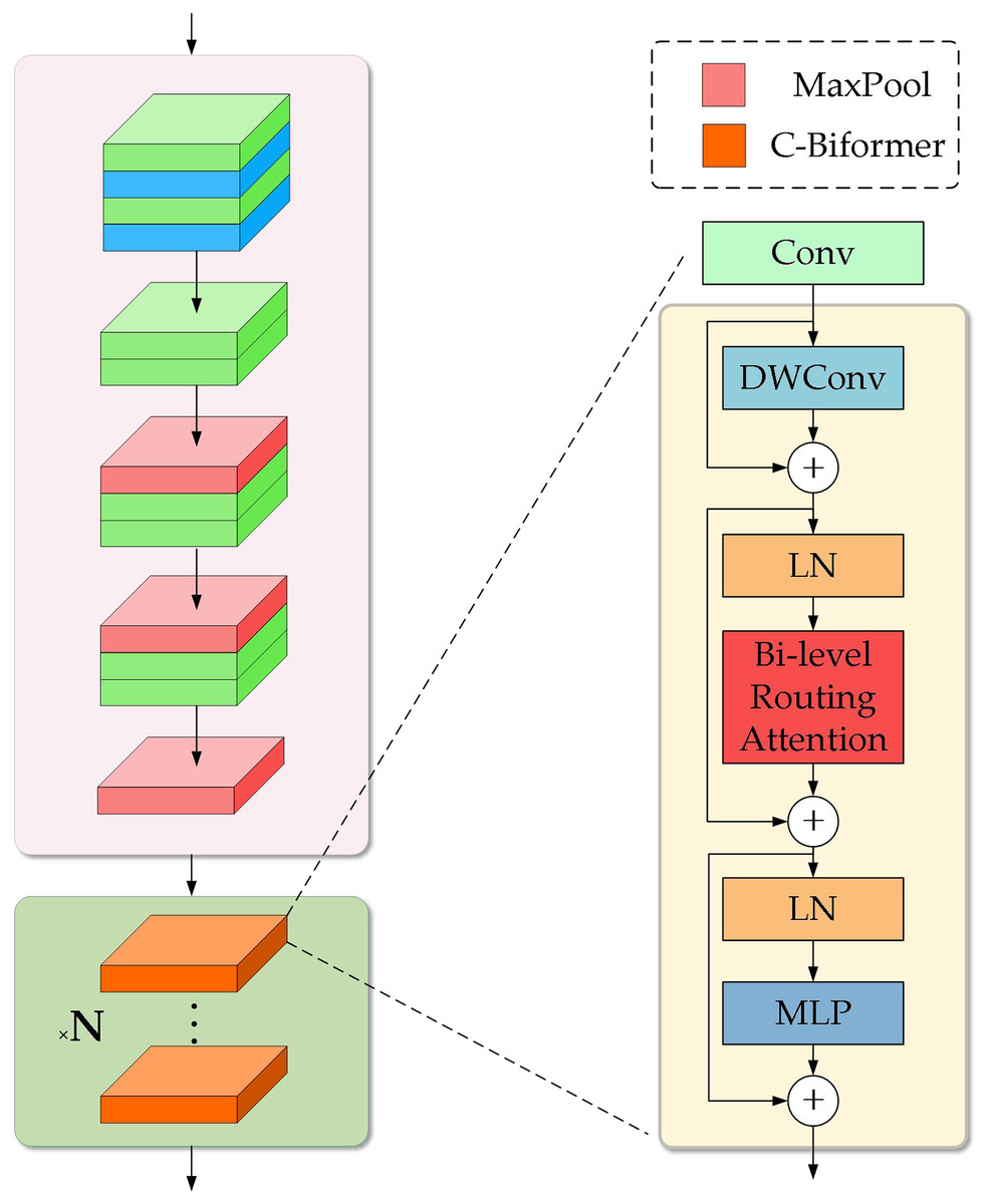
Figure 4: C-BiFormer module and improved model structure.
Gas plume targets have no obvious contour information, elongated morphological features with less texture, and simpler morphology compared to general visual targets. Therefore, using a complex feature extraction network may pay too much attention to the details of the input image, leading to the extraction of unnecessarily complex features on targets with simple textures, while ignoring the overall structure and shape information of the target, affecting the accuracy of detection and segmentation. Therefore, in the backbone network structure of the model, we remove the ELAN structure in YOLOv7 and define the newly proposed model structure as YOLOv7-CB. As shown on the left side in Fig. 4, at the beginning of the model, the four-layer standard convolution is still used to perform the initial feature transformations and information filtering, which helps the network to make a smooth transition from low-level features to high-level semantic information. In the next three layers of the ELAN structure, each of them is replaced by two layers of standard convolution with a convolution kernel size of 3. On the one hand, this reduces the complexity of the model and avoids the risk of overfitting, and on the other hand, it can be more suitable for the extraction of simple textures by the model. The main feature extraction part we set at the last ELAN module in the backbone network. By stacking C-BiFormer modules with varying depths to replace the original ELAN module, we progressively expand the model’s receptive field and enhance multi-scale feature extraction capabilities. This approach maintains operational simplicity while improving overall model performance. In addition, we similarly replace the complex MPConv structure in the original model using ordinary maximum pooling to further simplify the model structure.
Experiment and analysis
Preliminary preparation
Dataset preparation
In this article, the raw data are obtained from a Kongsberg EM710 multibeam bathymetry system measurement with a beam opening angle of about 120°, and the Seafloor Information System (SIS) acquisition software is used for data acquisition and storage. For the measured multibeam water column data, after quantifying the grayscale values using the backscattering intensity information, 320 water column images containing gas plume targets are obtained. The dataset is then divided at a ratio of 8:1:1, and data augmentation operations such as translation, rotation, and MixUp are carried out. Ultimately, 1,920 images are generated for training, validation, and testing. To meet the data requirements of the YOLO format, we use Labelme software to create the dataset labels.
Experimental environment
We conduct our experiments on the Ubuntu 18.04.5 operating system, equipped with a V100 graphics card and an Intel Xeon Processor CPU with 10 virtual cores, along with 32 GB of graphics memory and 72 GB of RAM. The GPU is accelerated using CUDA 11.1, and all the network models are built using Python 3.8 and Torch 1.8.1 within Visual Studio Code 1.75.1. To highlight the effect of the models proposed in this article, we use the same hyperparameters for all networks, and the specific settings are shown in Table 1.
| Hyperparameter | Configuration |
|---|---|
| Initial learn rate | 0.01 |
| Optimizer | SGD |
| Weight decay | 0.0005 |
| Momentum | 0.937 |
| Image size | 480 × 480 |
| Batch size | 32 |
| Epochs | 300 |
Model evaluation metric
In the improved model related to the transformer, due to the higher computational complexity of the self-attention mechanism, the model needs to process more computations and consume more resources. Therefore, the article uses the number of parameters, computation, frames per second (FPS), GPU memory usage and weight size to evaluate the model’s scale change. Among the accuracy metrics, we use F1, mAP50, and mAP50:95 to evaluate the effectiveness of the model in detecting and segmenting gas plume targets, respectively. In the target detection task, the Intersection over Union (IoU) between the predicted box and the real box is first calculated, and when the IoU is greater than a set threshold then the predicted box is considered to match the real box. Precision, recall, and F1 values are calculated based on the matching results and AP is calculated based on the area under the Precision-Recall curve at different IoU thresholds. mAP denotes the average accuracy of all targets. However, there is only one plume target in this article, so . mAP50 denotes the accuracy metric computed when the IoU threshold is 50, and mAP50:95 indicates that the IoU threshold is between 50 and 95, and the precision is calculated and averaged every five thresholds, which reflects the model’s ability to detect under high threshold requirements. The target segmentation task is to replace the prediction box and the real box with the prediction mask and the real mask and to calculate the segmentation metrics under different IoU thresholds according to the degree of overlap between the prediction mask and the real mask. The specific formulas are shown below (where TP, FP, and FN denote true positive, false positive, and false negative, respectively):
(4)
(5)
(6)
(7)
Experimental analysis
Selection of baseline network and comparison of backbone networks
In this article, the segmentation network of YOLOv7 is selected as the improved baseline network, and the segmentation network of YOLOv7 can achieve the detection and segmentation of the target simultaneously, which not only retains the advantage of fast inference in the YOLO series but also shares the same part of feature extraction and maintains the consistency of features. Compared with the network that performs detection and segmentation separately, the simultaneous detection and segmentation results have more comprehensive target information, achieving more accurate target localization and reducing the possibility of misdetection and missed detection. During the improvement process, we conduct a large number of ablation and comparison experiments and evaluate them using previously introduced metrics to comprehensively verify the superiority of the YOLOv7-CB network proposed in this article. To better adapt to the morphological characteristics of the gas plume target, in this article, we first prune for the backbone network. As shown in Fig. 5, we sequentially replace the ELAN structure in the backbone network with two layers of standard convolution. From Table 2, it can be seen that with the reduction of the ELAN structure, the network is sequentially improved in each scale metric. In terms of accuracy (as shown in Table 3), retaining only one ELAN structure in the deep network achieves performance beyond the baseline. In the detection task, YOLOv7-1ELAN increased by 1.5%, 1.7%, and 0.2% over baseline on F1, mAP50, and mAP50:95, and by 1.7%, 4.7%, and 0.6% in the segmentation task, respectively. For the module at the shallow layer of the network, the extracted features are mostly the underlying features, such as edges and textures. Ordinary convolution has a certain ability in extracting underlying features. Replacing the first three ELAN modules with ordinary convolution can remove redundant features and make the model focus more on semantic features with distinguishing degree, thus improving accuracy.
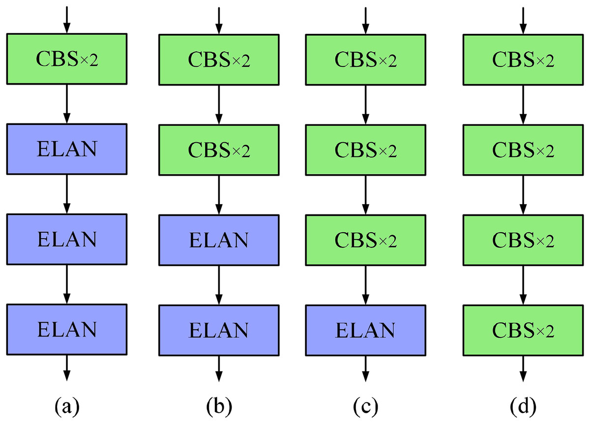
Figure 5: Comparison of pruned backbone networks.
(A) Three ELAN structures are retained (i.e., 3ELAN). (B) Two ELAN structures are retained (i.e., 2ELAN). (C) One ELAN structure is retained (i.e., 1ELAN). (D) No ELAN structure is retained (i.e., 0ELAN).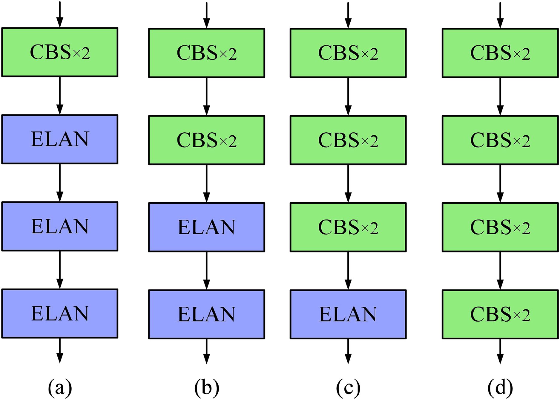
| Model | Params. (M) | FLOPs (G) | FPS | GPU memory (G) | Weight (MB) |
|---|---|---|---|---|---|
| YOLOv7 | 37.8 | 141.9 | 67.1 | 15.9 | 72.6 |
| YOLOv7-3ELAN | 37.6 | 129.4 | 69.9 | 14.7 | 72.1 |
| YOLOv7-2ELAN | 36.5 | 116.3 | 74.6 | 13.8 | 70.0 |
| YOLOv7-1ELAN | 32.0 | 103.2 | 76.9 | 13.3 | 61.6 |
| YOLOv7-0ELAN | 27.9 | 99.8 | 78.7 | 13.2 | 53.6 |
| Model | Box | Mask | ||||
|---|---|---|---|---|---|---|
| F1 (%) | mAP50 (%) | mAP50:95 (%) | F1 (%) | mAP50 (%) | mAP50:95 (%) | |
| YOLOv7 | 94.6 | 96.0 | 51.1 | 86.8 | 83.9 | 34.4 |
| YOLOv7-3ELAN | 94.5 | 96.6 | 50.2 | 85.3 | 84.1 | 33.0 |
| YOLOv7-2ELAN | 93.2 | 95.8 | 50.0 | 87.2 | 88.2 | 35.0 |
| YOLOv7-1ELAN | 96.1 | 97.7 | 51.3 | 88.5 | 88.6 | 35.0 |
| YOLOv7-0ELAN | 94.1 | 97.6 | 51.1 | 86.6 | 85.0 | 33.9 |
Design and analysis of the YOLOv7-CB network architecture
The ELAN structure achieves better expressiveness by aggregating different hierarchical features, but its expressiveness is still limited by the local context. Therefore, in this article, we use the proposed C-BiFormer module to replace the ELAN structure in YOLOv7-1ELAN by stacking, so that the network can do global modeling while acquiring local features, which has better interpretability compared with the ELAN structure. We design two network structures with different scales, as shown in Tables 4 and 5. In the first network structure, YOLOv7-CBs, we comprehensively outperform the baseline network in terms of scale and accuracy by stacking only four layers of C-BiFormer modules. The number of parameters, FLOPs, GPU memory and weight size are reduced by 45.5%, 32.7%, 25.2% and 45.3% respectively, and the FPS is increased by 2.3, with the network having faster inference. In the detection task, F1 has the same accuracy as the baseline, but in mAP50 and mAP50:95, it increases by 0.8% and 1.1% respectively. In the segmentation task, F1, mAP50, and mAP50:95 increased by 0.6%, 3.7%, and 1.4% respectively. The results show that using only four-layer C-BiFormer can adapt well to the morphological characteristics of the gas plume target, which is mainly attributed to the internal sparse attention, which can quickly exclude irrelevant regions, and the use of self-attention, which can focus more on the features related to the gas plume. Although similar to YOLOv7-1ELAN in terms of accuracy metrics, the four-layer C-BiFormer is smaller in terms of model size and is able to perform inference tasks more efficiently with limited resources. In the second network structure, YOLOv7-CBl, we stacked 12 layers of C-BiFormer modules, allowing the network to significantly outperform the baseline network in terms of accuracy. In the detection task, F1, mAP50, and mAP50:95 increased by 3.9%, 3.4%, and 1.6% respectively. In the segmentation task, F1, mAP50, and mAP50:95 increased by 5.4%, 7.9%, and 1.9% respectively. And in terms of the number of parameters, FLOPs, GPU memory and weight size, the 12-layer C-BiFormer is still reduced by 44.2%, 28.5%, 23.3% and 44.1% respectively. By stacking multiple C-BiFormer modules, the model can analyze input from multiple views and layers, learn more complex features and patterns, and make the overall model structure more flexible, retaining more design space and scalability. However, in terms of inference speed, the new model is slower, mainly because the long-distance dependencies in the feature maps need to take into account more relationships between regions, and the deeper the layers, the longer the inference time.
| Model | Params. (M) | FLOPs (G) | FPS | GPU memory (G) | Weight (MB) |
|---|---|---|---|---|---|
| YOLOv7-CBs | 20.6 | 95.5 | 69.4 | 11.9 | 39.7 |
| YOLOv7-CBl | 21.1 | 101.5 | 46.3 | 12.2 | 40.6 |
| Model | Box | Mask | ||||
|---|---|---|---|---|---|---|
| F1 (%) | mAP50 (%) | mAP50:95 (%) | F1 (%) | mAP50 (%) | mAP50:95 (%) | |
| YOLOv7-CBs | 94.6 | 96.8 | 52.2 | 87.4 | 87.6 | 35.8 |
| YOLOv7-CBl | 98.5 | 99.4 | 52.7 | 92.2 | 91.8 | 36.3 |
To further analyze the effectiveness of the proposed modules and the constructed model, we plotted the effective receptive field (ERF) heatmap (Ding et al., 2022) of the backbone in the model. As shown in Fig. 6, the dark regions represent the ERF size and pixel contribution levels. YOLOv7 exhibits a smaller ERF, with high-contribution pixels concentrated around the center and minimal edge influence. In contrast, YOLOv7-CBs and YOLOv7-CBl demonstrate significantly expanded ERFs, with YOLOv7-CBl showing more uniform distribution of high-contribution pixels, indicating stronger spatial information aggregation capabilities. Based on this, we conducted in-depth quantitative analysis. As shown in Table 6, “t” represents the threshold of contribution scores, indicating the minimum area coverage ratio of top t% high-contribution pixels in the final prediction results. The corresponding values represent the proportion of this minimum area to the entire image. As the threshold t increases, the area coverage ratios of YOLOv7 to YOLOv7-CBl sequentially increase, reflecting expanding ERFs. At t = 20%, YOLOv7-CBl achieves 15.1% coverage, enabling more effective integration of regional information for small object feature extraction. At t = 99%, the ratio reaches 97.8%, indicating that most image information contributes significantly to the final prediction, facilitating better large object information capture. In this article, C-Biformer module is used to build the model, which has a larger effective receptive field than ELAN module. With the increase of model depth, the receptive field gradually increases, which enhances the multi-scale feature extraction ability of the model.
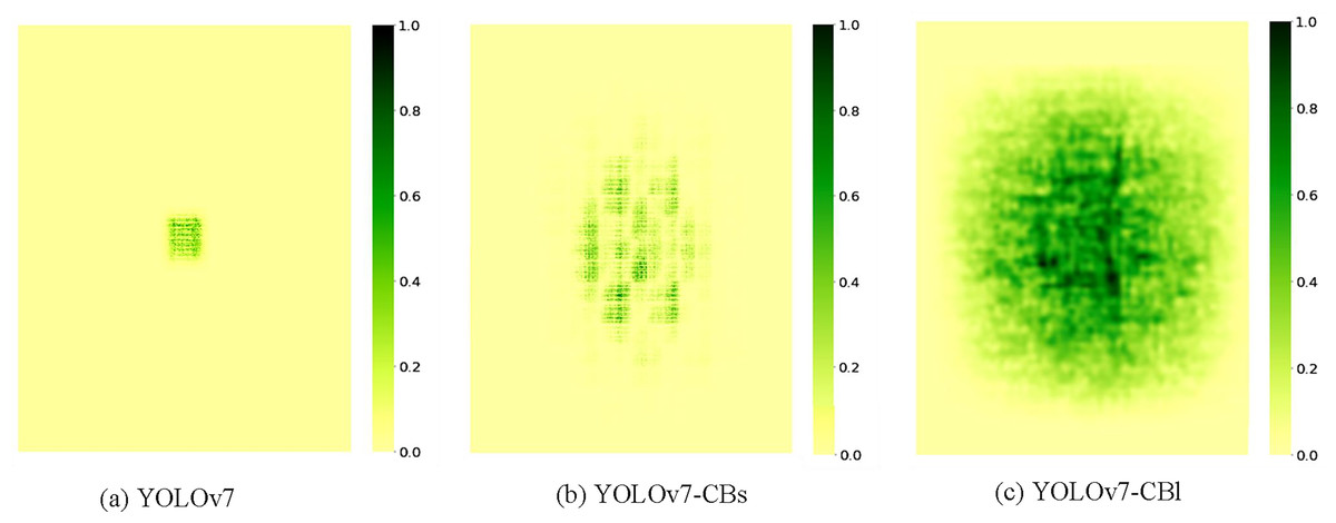
Figure 6: (A–C) Visualized heatmaps of the receptive fields before and after the improvement.
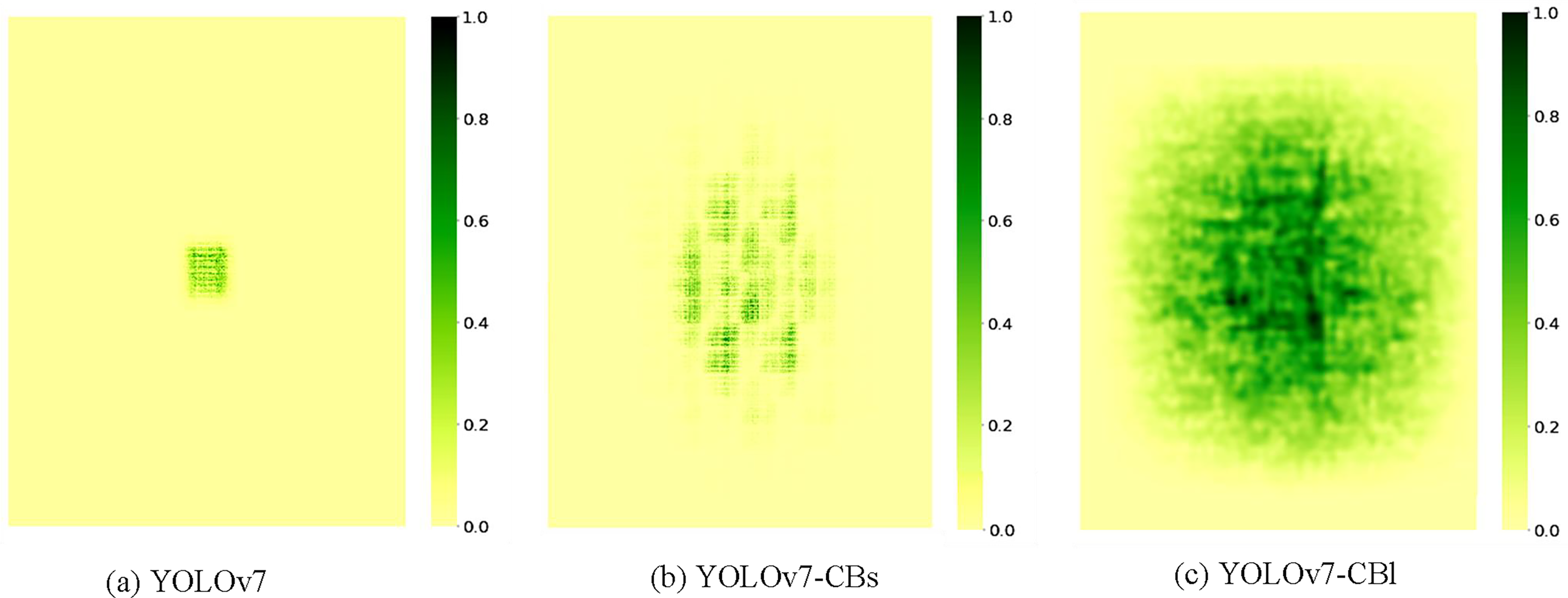
| Model | t = 20% | t = 30% | t = 50% | t = 99% |
|---|---|---|---|---|
| YOLOv7 | 0.2 | 0.3 | 0.5 | 16.6 |
| YOLOv7-CBs | 3.5 | 5.4 | 8.4 | 86.4 |
| YOLOv7-CBl | 15.1 | 23.0 | 28.9 | 97.8 |
Comparison of the proposed method with other self-attention modules
To verify the superiority of the C-BiFormer module in various aspects, we replace the C-BiFormer module with self-attentive modules such as ViT (Dosovitskiy et al., 2020), Swin transformer (Liu et al., 2021b), Conv2former (Hou et al., 2022), and Contextual Transformer (CoT) (Li et al., 2023a), respectively, based on YOLOv7-CBl. ViT and Swin transformer are purely self-attentive modules that require more hardware resources. As shown in Table 7, ViT and Swin transformer have relatively high requirements in terms of the number of parameters, FLOPs, and GPU memory. Conv2former, CoT, and C-BiFormer are all methods that use convolutional operations to simplify or simulate self-attention and therefore have a relatively low resource footprint. Among them, C-BiFormer has the fastest inference speed and the same lowest number of parameters, while CoT shows better results in terms of FLOPs and GPU memory usage, which is because CoT mainly uses a 3 × 3 convolution operation to encode the context of key points, an operation that only involves key points in local neighborhoods and does not need to operate on the whole input feature map, reducing the computation and reduces the memory usage. In terms of model accuracy, YOLOv7-CBl shows the best results in all metrics, as shown in Table 8. F1, mAP50, and mAP50:95 outperform the second-ranked CoT by 2.9%, 1.8%, and 1.3% in the detection task and by 2.8%, 1.7%, and 0.1% in the segmentation task. Although CoT also achieves relatively good results with dynamic sparse attention as the starting point of module design, the range of contexts acquired by the 3 × 3 convolution operation is still limited, so CoT performs slightly worse than C-BiFormer when dealing with targets with elongated morphology such as gas plumes. The low accuracy of the other modules is because ViT directly splits the feature map into fixed-size image patches during the input process without any inductive bias, resulting in a model that does not adapt well to the morphological features of the gas plume target. Swin transformer, although it adopts a hierarchical approach to capture the multi-scale features, for some small-size and feature-less gas plume targets, may not be able to capture enough detailed information. Conv2Former adopts static convolution to simulate self-attention but fails to achieve the adaptive function in self-attention well.
| Model | Params. (M) | FLOPs (G) | GPU memory (G) | FPS |
|---|---|---|---|---|
| +ViT block | 22.7 | 93.9 | 17.2 | 25.8 |
| +Swin transformer block | 21.5 | 124.5 | 12.3 | 44.2 |
| +Conv2former block | 21.2 | 93.3 | 11.8 | 40.8 |
| +CoT block | 21.1 | 93.2 | 11.6 | 42.4 |
| YOLOv7-CBl | 21.1 | 101.5 | 12.2 | 46.3 |
| Model | Box | Mask | ||||
|---|---|---|---|---|---|---|
| F1 (%) | mAP50 (%) | mAP50:95 (%) | F1 (%) | mAP50 (%) | mAP50:95 (%) | |
| +ViT block | 94.6 | 97.2 | 51.8 | 87.5 | 87.9 | 34.3 |
| +Swin transformer block | 94.9 | 94.0 | 52.7 | 88.9 | 88.3 | 36.1 |
| +Conv2former block | 85.6 | 89.7 | 40.5 | 79.2 | 80.3 | 28.7 |
| +CoT block | 95.6 | 97.6 | 51.4 | 89.4 | 90.1 | 36.2 |
| YOLOv7-CBl | 98.5 | 99.4 | 52.7 | 92.2 | 91.8 | 36.3 |
Comparison of the proposed method with other common attention modules
To compare the accuracy between self-attention and common attention, we conduct experiments using four types of common attention mechanisms: Squeeze-and-Excitation (SE) (Hu, Shen & Sun, 2018), Convolutional Block Attention Module (CBAM) (Woo et al., 2018), Efficient Multi-scale Attention (EMA) (Ouyang et al., 2023), and Normalization-based Attention Module (NAM) (Liu et al., 2021a). As shown in Table 9, conventional attention modules enhance the model’s sensitivity to different features by learning relationships between channels or spatial elements, thus improving performance. The related improvement methods are also focusing on weight computation and cross-dimensional interactions. Although they require lower computational resources, they still emphasize local information and are more suitable for specific tasks. These methods show lower accuracy in the experimental results of this study. On the other hand, C-BiFormer’s position invariance is more versatile, preserving not only local features but also achieving global information interaction through self-attention. Furthermore, common attention modules often suffer from information bottleneck problems when stacked repeatedly in the model, causing the model to overly focus on channel or spatial information while disregarding contextual information. The residual connections and LN within the C-BiFormer module effectively address this problem, resulting in overall higher performance.
| Model | Box | Mask | ||||
|---|---|---|---|---|---|---|
| F1 (%) | mAP50 (%) | mAP50:95 (%) | F1 (%) | mAP50 (%) | mAP50:95 (%) | |
| +SE block | 94.8 | 95.9 | 51.6 | 87.3 | 86.7 | 36.1 |
| +CBAM block | 95.7 | 96.0 | 52.0 | 85.0 | 82.2 | 33.6 |
| +EMA block | 94.0 | 95.4 | 50.7 | 86.8 | 87.7 | 34.4 |
| +NAM block | 95.8 | 96.3 | 51.9 | 88.6 | 89.2 | 34.5 |
| YOLOv7-CBl | 98.5 | 99.4 | 52.7 | 92.2 | 91.8 | 36.3 |
Analysis of ablation experiments based on YOLOv7-CB
The bi-level routing attention in C-BiFormer retains the top k most relevant regions in each region after coarse screening of the partitioned regions. Therefore, the size of k determines the sparsity and computational overhead of the model. In this article, we adjust the size of k so that the model can strike a balance between the relevance of regions and computational overhead. As shown in Table 10, we set four different values of k = 1, 2, 4, 8 for the experiment. Although the overall result is greatly improved compared to the baseline, but when k = 1 or 2, the connection graph is too sparse to capture some important correlation information; when k = 8, the connection graph is more dense and can capture more correlation information. Good results are obtained in some metrics, but more computational resources are used. All things considered, we choose k = 4 as the final correlation value, so that the model can maintain a good result in both precision and computational overhead.
| Top k | Box | Mask | ||||
|---|---|---|---|---|---|---|
| F1 (%) | mAP50 (%) | mAP50:95 (%) | F1 (%) | mAP50 (%) | mAP50:95 (%) | |
| 1 | 96.4 | 98.3 | 51.6 | 91.3 | 89.9 | 35.5 |
| 2 | 96.6 | 98.9 | 51.7 | 88.9 | 87.2 | 34.6 |
| 4 | 98.5 | 99.4 | 52.7 | 92.2 | 91.8 | 36.3 |
| 8 | 97.2 | 98.4 | 52.8 | 88.6 | 88.9 | 36.5 |
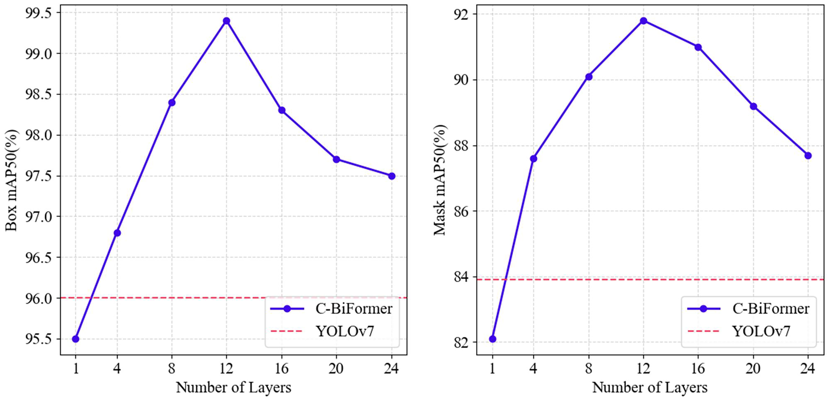
YOLOv7-CB consists of multiple C-BiFormer modules stacked on top of each other, and in the second ablation experiment, we mainly evaluate the effect of the number of module stacks on the model performance. As shown in Fig. 7, we set the number of modules from 1 to 24 layers and evaluate them every four layers to see the trend of the model on mAP50. With only one layer of the C-BiFormer module, the accuracy of the new model is below the baseline, but when adding up to four layers, the model already outperforms the baseline in both the detection and segmentation tasks and grows rapidly in the subsequent process. After stacking 12 layers, the model reaches maximum performance and begins to show performance saturation. As the number of modules increases, so does the depth of the network, and the model begins to reuse similar features, resulting in redundancy when information is propagated between different layers, and the performance of the model cannot be further improved. In addition, due to the attention collapse (Zhou et al., 2021) problem of deep Transformer, the model cannot distinguish between important and secondary information, and the long-distance dependent modeling ability decreases. The enhancement of the receptive field will introduce more background noise in the deeper network, which will interfere with the key feature extraction and lead to the reduction of accuracy. However, the downward trend is slow, and at 24 layers, the model accuracy is still higher than the baseline. The results show that YOLOv7-CB is highly flexible and can maintain good performance after stacking C-BiFormer modules several times.
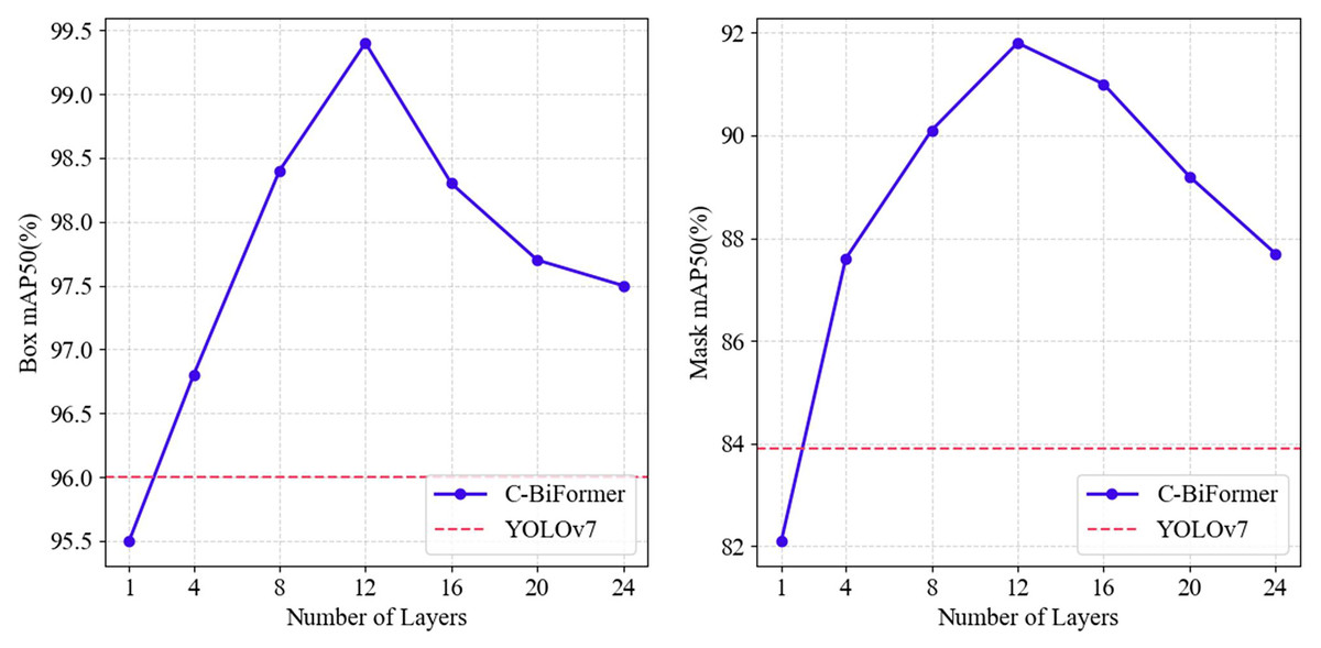
Figure 7: The mAP50 variation curve of C-BiFormer modules with different quantities in YOLOv7-CB.
Experimental analysis of the proposed method with other state-of-the-art networks
In comparison with other SOTA (state-of-the-art) models, we select some networks that can achieve both target detection and segmentation for comparison experiments, e.g., YOLOv5 (Jocher et al., 2022), YOLOv8 (Ultralytics, 2023), YOLOv9 (Wang et al., 2024), YOLO11 (Ultralytics, 2024), YOLACT (You Only Look At CoeffificienTs) (Bolya et al., 2019), Mask R-CNN (He et al., 2017), and Cascade Mask R-CNN (Cai & Vasconcelos, 2018). From Table 11, it can be seen that in the detection task, the YOLO series network shows higher accuracy. This is mainly due to the continuous iteration and optimization of the YOLO series, which introduces the most advanced network architecture and training techniques, along with data augmentation and sample balancing strategies. These factors enable the network to extract richer features, and the improved network performs the best in all detection metrics. However, in the segmentation task, the accuracy of mAP50:95 is lower than that of YOLACT, Mask R-CNN, and Cascade Mask R-CNN, which are specifically used for segmentation. The reasons are: the concept of ProtoNet is introduced in YOLACT to represent the feature prototypes of the objects and reduce the segmentation error, Mask R-CNN takes advantage of the precise feature alignment provided by ROIAlign, which is more helpful in capturing the boundary and shape of the target, while Cascade Mask R-CNN gradually screens candidate targets through a cascade structure so that each stage focuses on processing targets with different levels of difficulty, thus being able to maintain good accuracy despite high thresholds.
| Model | Box | Mask | ||||
|---|---|---|---|---|---|---|
| F1 (%) | mAP50 (%) | mAP50:95 (%) | F1 (%) | mAP50 (%) | mAP50:95 (%) | |
| YOLOv5m | 95.4 | 95.2 | 47.8 | 85.7 | 84.9 | 34.3 |
| YOLOv8m | 91.3 | 93.8 | 50.7 | 72.5 | 71.5 | 34.5 |
| YOLOv9c | 94.2 | 96.5 | 51.8 | 88.2 | 86.7 | 35.4 |
| YOLO11m | 92.7 | 96.0 | 51.0 | 89.1 | 87.3 | 35.2 |
| YOLACT | 89.2 | 88.7 | 46.8 | 75.5 | 72.8 | 37.4 |
| Mask R-CNN | 85.7 | 78.6 | 42.0 | 84.5 | 77.0 | 39.4 |
| Cascade mask R-CNN | 85.3 | 78.3 | 52.6 | 85.5 | 78.9 | 51.9 |
| Ours | 98.5 | 99.4 | 52.7 | 92.2 | 91.8 | 36.3 |
Detection and segmentation results of gas plume targets in multibeam water column images
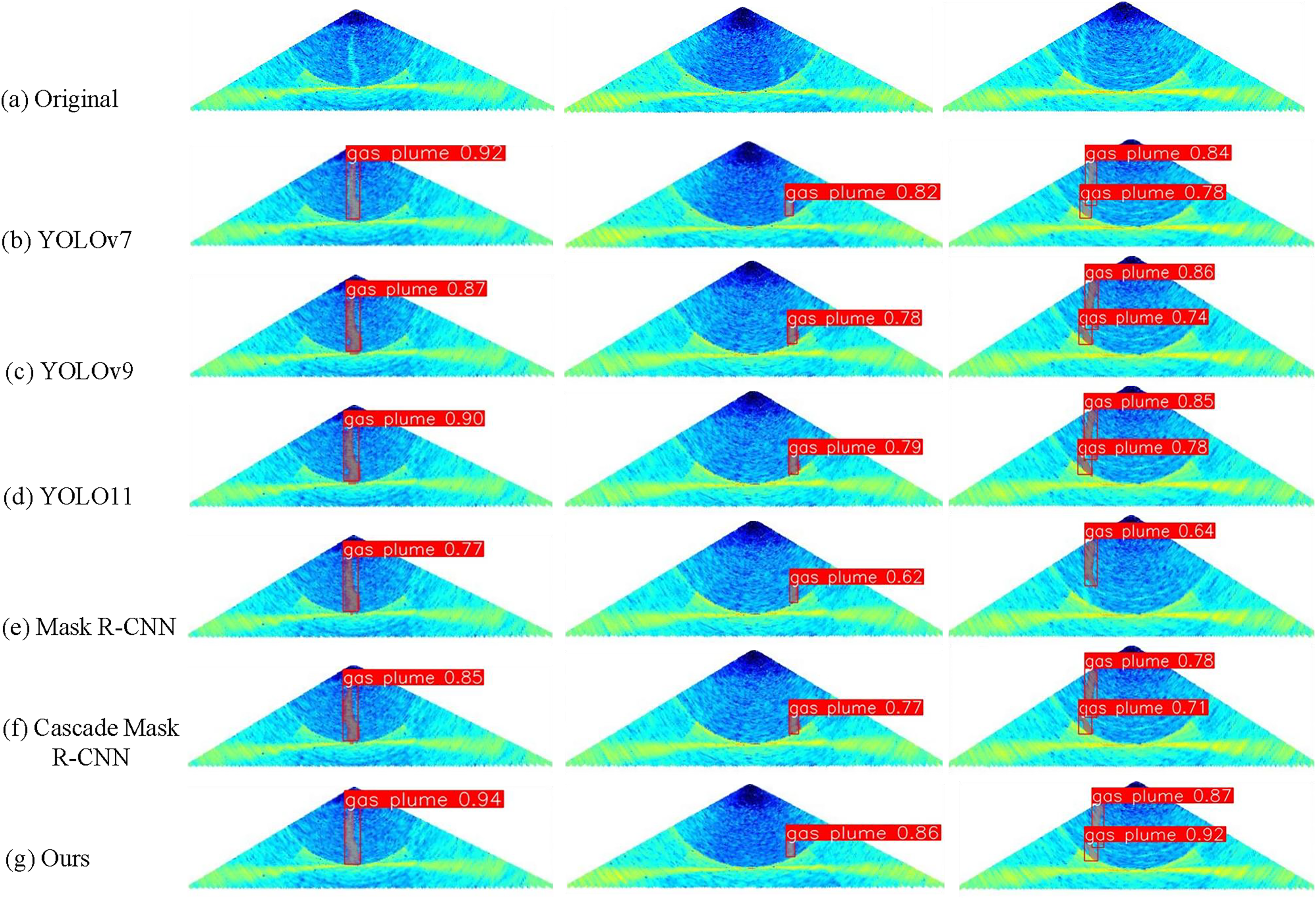
At the end of the experiment, we select some plume target images with different scales and characteristics for instance testing, and make a more intuitive comparison of the performance gap between YOLOv7-CBl and other state-of-the-art (SOTA) models. As shown in Fig. 8, the first column shows clear plume targets, which exhibit higher detection accuracy and consistent segmentation results under the detection and segmentation of YOLOv7-CBl. The second column consists of small plume targets. Some models are unable to perform complete segmentation well, and in terms of detection, YOLOv7-CBl demonstrates higher detection accuracy. The plume targets in the third column are affected by sidelobe noise, resulting in being divided into two segments after imaging. However, YOLOv7-CBl is less affected by the noise, and it can still perceive the morphological features of the targets well, with higher accuracy and more complete segmentation results. The experimental results show that YOLOv7-CBl can be better adapted to the performance morphology of the gas plume target on the seafloor as well as to the noise defects in multibeam water column images, which improves the application of multibeam WCI in target detection and segmentation.
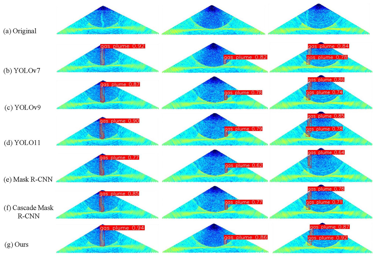
Figure 8: (A–G) Comparison of detection and segmentation results of different models.
Conclusions
To better adapt to the characteristics of the multibeam WCI, where the gas plume target has elongated morphology, fuzzy boundaries, and high noise influence, we propose a network structure combining CNN and transformer based on the YOLOv7 segmentation model: YOLOv7-CB. Firstly, we sequentially reduce the ELAN structure in the backbone network to simplify the network and conclude that the complex network structure is prone to lead to the overfitting problem when feature extraction is performed on gas plume targets with only simple textures. Using the ELAN module only in the deep network is better able to meet the feature extraction needs of gas plume targets, thus showing higher accuracy. Secondly, we propose the C-BiFormer module, by combining the convolutional module with the BiFormer module, which not only makes up for the shortcomings of local feature extraction but also uses self-attention to capture the distant correlations and enhance the perception of global information. Moreover, the bi-level routing attention in BiFormer can filter irrelevant regions in the image, and only compute the self-attention in the regions related to the target, reducing both model size and memory occupation. Finally, the C-BiFormer module replaces the last ELAN module in the backbone network and gradually extracts different levels of abstract features by stacking to learn in depth the complex semantic relationships in the image, showing high detection and segmentation accuracies in all experimental results. However, due to the deepening of the model depth, the deep Transformer module is prone to attention collapse, which makes the self-attention head of Transformer pay more attention to the background area, resulting in noise accumulation, which makes it difficult to improve the accuracy of the model, and even reduce the situation. In the future work, we will further improve the model structure, introduce cross-stage feature reuse through skip joining, pruning and other methods to reduce redundant features and improve model efficiency.