
An improved hippopotamus optimization algorithm based on adaptive development and solution diversity enhancement
- Published
- Accepted
- Received
- Academic Editor
- Bilal Alatas
- Subject Areas
- Algorithms and Analysis of Algorithms, Optimization Theory and Computation, Neural Networks
- Keywords
- Hippopotamus optimization algorithm, Adaptive exploitation, Solution diversity, Chaotic mapping, Global optimization
- Copyright
- © 2025 Pei et al.
- Licence
- This is an open access article distributed under the terms of the Creative Commons Attribution License, which permits unrestricted use, distribution, reproduction and adaptation in any medium and for any purpose provided that it is properly attributed. For attribution, the original author(s), title, publication source (PeerJ Computer Science) and either DOI or URL of the article must be cited.
- Cite this article
- 2025. An improved hippopotamus optimization algorithm based on adaptive development and solution diversity enhancement. PeerJ Computer Science 11:e2901 https://doi.org/10.7717/peerj-cs.2901
Abstract
This study proposes an improved hippopotamus optimization algorithm to address the limitations of the traditional hippopotamus optimization algorithm in terms of convergence performance and solution diversity in complex high-dimensional problems. Inspired by the natural behavior of hippopotamuses, this article introduces chaotic map initialization, an adaptive exploitation mechanism, and a solution diversity enhancement strategy based on the original algorithm. The chaotic map is employed to optimize the initial population distribution, thereby enhancing the global search capability. The adaptive exploitation mechanism dynamically adjusts the weights between the exploration and exploitation phases to balance global and local searches. The solution diversity enhancement is achieved through the introduction of nonlinear perturbations, which help the algorithm avoid being trapped in local optima. The proposed algorithm is validated on several standard benchmark functions (CEC17, CEC22), and the results demonstrate that the improved algorithm significantly outperforms the original hippopotamus optimization algorithm and other mainstream optimization algorithms in terms of convergence speed, solution accuracy, and global search ability. Moreover, statistical analysis further confirms the superiority of the improved algorithm in balancing exploration and exploitation, particularly when dealing with high-dimensional multimodal functions. This study provides new insights and enhancement strategies for the application of the hippopotamus optimization algorithm in solving complex optimization problems.
Introduction
With the continuous advancements in science, industry, and technology, many problems are defined as optimization problems (Chen et al., 2024a). These problems typically consist of three fundamental components: an objective function, constraints, and decision variables (Zhang et al., 2022). To address such challenges, optimization algorithms can be classified into various categories. One common classification distinguishes between stochastic and deterministic algorithms based on their inherent optimization approach. Unlike deterministic methods, stochastic approaches do not require comprehensive knowledge of the problem’s characteristics, making them advantageous when dealing with complex, high-dimensional, nonlinear, and non-differentiable problems. Stochastic methods are especially effective when the problem is poorly understood or treated as a black box (Ju & Liu, 2024).
Among the numerous stochastic methods, metaheuristic algorithms have garnered significant attention due to their exceptional performance in solving complex problems (Dai & Fu, 2023; Dong & Chen, 2023). These algorithms generate an initial set of candidate solutions randomly and iteratively update these solutions according to specific relationships defined by the algorithm. In each iteration, better solutions are retained based on the number of search agents until a termination criterion, such as a predefined maximum number of iterations or the number of function evaluations, is met. The advantage of metaheuristic algorithms lies in their ability to balance global and local search, allowing them to excel in various applications (Guo, 2023; Chen, 2023; Zhang, 2023).
The hippopotamus optimization algorithm (HO) is a nature-inspired metaheuristic optimization algorithm first introduced in 2024 by Amiri et al. (2024). The HO draws inspiration from three behavioral patterns observed in hippopotamuses: position updates in water, defensive strategies against predators, and predator evasion. These behaviors are mathematically modeled to guide the optimization process. Although many optimization algorithms have been proposed, the “No Free Lunch” (NFL) theorem suggests that no single algorithm can outperform all others in solving every optimization problem. As increasingly complex optimization problems arise, traditional algorithms often struggle to handle issues such as nonlinearity, non-convexity, and non-differentiability. The HO was designed to balance global exploration and local exploitation by simulating hippopotamus behavior, thereby enhancing convergence speed and solution accuracy in multi-dimensional, multi-modal optimization problems. Despite the HO’s strong performance in benchmark tests and practical applications, it still faces certain limitations common to metaheuristic algorithms (Mashru et al., 2024). Therefore, developing novel and efficient optimization algorithms remains a critical research focus (Trojovsky & Dehghani, 2022).
Metaheuristic algorithms have found widespread applications across various engineering fields, including hyperparameter tuning and neural network weight optimization in medical engineering, intelligent fault diagnosis in control engineering, controller parameter optimization in mechanical engineering, and filter design in telecommunications engineering (Liao et al., 2024; Dehghani & Trojovsky, 2021; Emami, 2022; Trojovsky & Dehghani, 2022; Chen, Niu & Zhang, 2022; Yu et al., 2023; Han et al., 2024). These algorithms have also proven valuable in energy, civil engineering, and economics.
Recent studies have shown that chaotic mapping can significantly enhance the performance of metaheuristic algorithms. The mountain gazelle optimizer (MGO) stands out for its fast convergence and high precision, but it suffers from premature convergence and is prone to being trapped in local optima. Sarangi & Mohapatra (2024) proposed the chaotic mountain gazelle optimizer (CMGO), which leverages multiple chaotic maps to overcome these limitations. The Harris hawks optimization (HHO) algorithm, a novel swarm-based nature-inspired algorithm, has exhibited excellent performance but still has the drawbacks of premature convergence and falling into local optima due to the imbalance between exploration and exploitation. Yang et al. (2023) proposed the HHO-cs-oelm algorithm, which enhances global search capability through chaotic sequences and strengthens local search capability via opposition-based elite learning, thereby balancing exploration and exploitation. The HHO, inspired by the unique foraging strategies and cooperative behavior of Harris hawks, is also prone to local optima and slow convergence. Almotairi et al. (2023) presented several techniques to enhance the performance of metaheuristic algorithms (MHAs) and address their limitations. Chaotic optimization strategies, which have been proposed for many years to enhance MHAs, include four different types: chaotic mapping initialization, stochasticity, iteration, and control parameters. This article introduces a novel hybrid algorithm, SHHOIRC, designed to improve the efficiency of HHO. An adaptive HHO algorithm based on three chaotic optimization methods has been proposed.
To address the shortcomings of existing algorithms in terms of convergence speed and solution accuracy, this article proposes an improved hippopotamus optimization algorithm, hereafter referred to as IHO. The IHO optimizes the process by simulating hippopotamus behaviors observed in nature. The main contributions and innovations of this study are as follows. In subsequent sections, the improved algorithm will be referred to consistently as IHO.
-
Introducing chaotic mapping for population initialization, which improves the diversity distribution of the population and enhances global search capability.
-
Designing an adaptive exploitation mechanism that dynamically adjusts the weights of the exploration and exploitation phases based on iterative information, balancing global and local searches.
-
Proposing a solution diversity enhancement strategy that introduces nonlinear perturbations, reducing the risk of trapping in local optima and further improving algorithm performance.
The effectiveness of the improved algorithm is validated through experiments on multiple benchmark functions. The results show that IHO outperforms the traditional HO and other mainstream optimization algorithms in terms of solution accuracy, convergence speed, and global search capability.
The structure of this article is organized as follows: “Related Work” reviews related work. “Hippopotamus Optimization Algorithm” introduces the fundamental HO. “Improved Hippopotamus Optimization Algorithm” describes the proposed improvements to the HO. “Experiment and Analysis” presents the simulation experiments and analysis of the results. Finally, “Conclusion” provides a conclusion and discusses future research directions.
Related work
In recent years, optimization algorithms have found widespread applications across various scientific and engineering fields, primarily due to their flexibility and adaptability in addressing complex, nonlinear, non-convex, and uncertain problems (Sun, 2024; Li, Lin & Liu, 2024; Fu, Dai & Wang, 2024; Sun & Ma, 2024; Ge, Xu & Chen, 2023). These algorithms are often inspired by natural phenomena and solve real-world problems by simulating various processes in nature. The inspirations behind these algorithms span biological evolution, physical and chemical laws, as well as collective behavior, human social dynamics, and game theory (Wang, 2024; Zhang, Wang & Ji, 2024; Zhang, 2024; Han, 2024; Gu et al., 2023; Wang, Li & Chen, 2024).
From different perspectives, optimization algorithms can be classified according to their objectives, decision variables, constraints, and sources of inspiration. Based on the type of objective, optimization algorithms can be categorized as single-objective, multi-objective, or many-objective. In terms of decision variables, they can be divided into continuous or discrete algorithms. Moreover, depending on whether constraints are imposed on the decision variables, optimization algorithms can be further classified as constrained or unconstrained. The diversity of sources of inspiration has led to the development of six major categories of optimization algorithms: evolutionary algorithms, physics- or chemistry-based algorithms, swarm intelligence-based algorithms, human behavior-based algorithms, game theory-driven algorithms, and mathematics-driven algorithms (Zhang et al., 2022; Zhao et al., 2023). Among these, swarm intelligence-based algorithms have gained significant attention for their efficiency and broad applicability in solving complex problems, making them a current research hotspot (Wang, 2024; Tong, 2024; Yang, 2024; Xu et al., 2023).
Swarm intelligence algorithms emulate the collective behaviors observed in animals, plants, and insects in nature, leading to the emergence of several classical algorithms (Amiri et al., 2024; Liu et al., 2024a; Yin et al., 2024). For instance, particle swarm optimization (PSO), inspired by the collective movements of bird flocks and fish schools, became one of the earliest and most widely applied algorithms. Ant colony optimization (ACO), which simulates the foraging behavior of ants, has demonstrated remarkable performance in path optimization problems. Additionally, the grey wolf optimization (GWO) and whale optimization algorithm (WOA) were inspired by the hunting strategies of grey wolves and the bubble-net feeding behavior of humpback whales, respectively, further expanding the application scope of swarm intelligence algorithms. Recently, emerging algorithms such as the beluga whale optimization (BWO) and African vultures optimization algorithm (AVOA) have also attracted research interest, showcasing ongoing innovation and development within the field of swarm intelligence.
In addition to swarm intelligence, optimization algorithms inspired by biological evolution and physical laws also play a significant role in optimization research (Amiri et al., 2024). Classical evolutionary algorithms such as genetic algorithm (GA), differential evolution (DE), and biogeography-based optimization (BBO) have shown exceptional performance across various domains. Physics-based algorithms, such as simulated annealing (SA), gravitational search algorithm (GSA), and multi-verse optimization (MVO), simulate physical phenomena, demonstrating adaptability and flexibility in different optimization scenarios (Chen et al., 2024b; Hou et al., 2023; Gong et al., 2023).
Moreover, algorithms inspired by human behavior and social dynamics have garnered widespread attention (Amiri et al., 2024; Chen, Niu & Zhang, 2022; Zheng et al., 2022; Zhao et al., 2023). For example, teaching-learning-based optimization (TLBO) and political optimizer (PO), based on teaching processes and political interactions, respectively, illustrate the unique advantages of human social behavior in solving optimization problems. Game theory-driven algorithms, such as squid game optimizer (SGO) and puzzle optimization algorithm (POA), simulate game rules and strategies, providing novel approaches to optimization.
As research continues to advance, new optimization algorithms are constantly emerging to address the limitations of existing ones, such as premature convergence and the imbalance between exploration and exploitation. For instance, the hippopotamus optimization algorithm (Amiri et al., 2024), a relatively recent method, integrates adaptive exploitation and solution diversity mechanisms, demonstrating significant advantages in solving complex problems. These innovations not only enhance algorithmic performance but also pave the way for future developments in optimization algorithms (Chen et al., 2024a; Liu et al., 2024b). However, like other stochastic metaheuristic algorithms, HO still faces common limitations. It cannot guarantee the global optimal solution due to its reliance on stochastic search strategies. Despite HO’s strong performance in certain problems, the NFL theorem suggests that it may not consistently outperform other optimization algorithms across all problems.
To overcome these limitations, this article proposes an improved hippopotamus optimization algorithm, which optimizes the problem-solving process by simulating the natural behaviors of hippopotamuses. Wang & Tian (2024) enhances the HO algorithm by integrating the Levy flight strategy based on the swarm-elite learning mechanism and the quadratic interpolation strategy. The aim is to improve its global search ability and information sharing among candidate solutions in PV model parameter extraction. The main improvement lies in the use of an elite retention strategy in the exploration phase, but the rebound in the defense and development phases is neglected. Our improvements start from the initialization of the population, introduce an adaptive strategy in the development phase, and employ Gaussian mutation and chaotic perturbation in the defense and escape phases. This approach enhances population diversity while avoiding the risk of being trapped in local optima.
Hippopotamus optimization algorithm
The workflow of the HO
This section introduces the fundamental HO. HO is inspired by the unique behaviors of hippopotamuses, incorporating their natural traits to address optimization challenges. By understanding the foundational principles and mechanisms of HO, we establish a basis for the subsequent improvements proposed in this study.
represents the updated individual position in update phase 1. This position is adjusted randomly based on the distance from the dominant hippopotamus (best solution) to explore the solution space.
(1) where the updated position of the -th individual in the first half of the population. is the current position of the -th individual. is the distance to the current global best position in the population. N is total number of individuals in the population. is number of dimensions in the solution space. is a random factor that influences the magnitude of the position update. is a weighting factor that controls the influence of the individual’s current position.
represents the updated individual position in update phase 1. When the temperature parameter T is high, this position is adjusted based on the dominant hippopotamus and the mean of a random group. When T is low, it is adjusted based on the difference between the mean and the dominant hippopotamus or randomly generated within the bounds.
(2) where B is a random scaling factor that influences the magnitude of the position update. is random numbers used to decide which movement rule to apply. , is the lower and upper bounds of the search space. is the mean position of a group of individuals, which serves as a reference for the update. is the distance to the best-performing (dominant) hippopotamus in the population. If , the position is updated with respect to the mean group position and the distance to the best-performing individual . Otherwise, a random position is generated within the bounds of the search space.
(3) where T is adaptive parameter that determines whether strong or weak exploitation is used. is a weight factor controlling the balance between exploration and exploitation. A is a random movement factor for controlling the exploration step size.
represents the updated individual position in the defense phase, adjusted based on the distance between the hippopotamus and the predator as well as the Levy flight strategy.
(4) and are the lower and upper bounds of the search space. The predator’s position is initialized randomly between the lower bound and upper bound in each dimension.
(5) where and are random variables drawn from normal distributions. This equation provides Levy that follow a heavy-tailed distribution, which is often used in stochastic optimization algorithms to allow both small and occasional large jumps for efficient exploration of the solution space.
(6) where denotes the gamma function. is the power-law index, where .
(7)
(8) where , , are random scaling coefficients sampled from uniform distributions. is a random angle within the range .
Levy flight RL is a common random walk model used to simulate animal foraging paths, and in this case, it’s represented as: . S is the number of search agents.D is the dimensionality. is the Levy exponent parameter.
represents the updated individual position in the escape phase, where positions are adjusted with local random perturbation within the range between the lower and upper bounds.
(9) where and represent the adaptive local lower and upper bounds for the hippopotamus positions, adjusting over iterations to focus the search progressively. represents the current iteration number in the optimization algorithm.
Detailed description of the three main phases
HO consists of three main stages: exploration, defense, and exploitation. Each phase plays a crucial role in balancing the search process between exploring the solution space broadly and refining around promising areas.
Exploration phase
In this phase, the candidate solutions (i.e., the positions of the hippopotamuses) are updated based on random vectors. The update rule is influenced by the current best solution (i.e., the position of the dominant hippopotamus) and random factors. This ensures the algorithm performs a global search across the solution space, preventing premature convergence to local optima. The position of each hippopotamus is updated using the Eqs. (1) and (3).
Defense phase
In this phase, the hippopotamuses simulate their defensive behavior when predators approach. They turn towards the predator and emit intimidating sounds to drive them away. This phase is designed for exploitation, where a local search is conducted around the current solution to identify better solutions nearby. The movement is modeled by random displacement vectors, allowing the hippopotamuses to make small movements within the search space, thereby refining the search. The defense phase is updated using Eq. (8).
Escape phase
When the hippopotamuses realize they cannot repel the predator, they choose to escape, typically towards the nearest body of water. This phase aims to help the algorithm escape from local optima by generating new solutions and moving to safer positions. The escape phase simulates the behavior of finding a safe zone and enhances the local search capability to improve solution quality. The escape phase is updated using Eq. (9).
To describe the structure of the standard HO, we can mention that the algorithm follows a clear, systematic process. As outlined in Algorithm 1, the flowchart visually represents the HO’s phases.
| 1: Input: Problem definition, maximum number of iterations Tmax, population size N |
| 2: Output: Optimal solution |
| 3: Step 1: Define the optimization problem: Specify the objective function and constraints |
| 4: Step 2: Initialize parameters: Set Tmax and N |
| 5: Step 3: Initialize population: Generate initial population of hippopotamuses and evaluate their objective function values |
| 6: for to Tmax do |
| 7: Update the dominant hippopotamus’s position: |
| 8: Update the global best solution Xbest based on the current objective function values |
| 9: First phase-Update hippopotamuses’ position in water: |
| 10: for to do |
| 11: Compute new positions using the update strategy Eqs. (1) and (3). |
| 12: Update position |
| 13: end For |
| 14: Second phase-Defend against predators: |
| 15: for to N do |
| 16: Randomly generate predator positions Pi |
| 17: Compute new positions considering Pi using Eq. (8) |
| 18: Update position |
| 19: end for |
| 20: Third phase-Escape from predators: |
| 21: for to N do |
| 22: Recompute the boundaries for decision variables |
| 23: Compute new positions based on new boundary conditions using Eq. (9) |
| 24: Update position |
| 25: end for |
| 26: Save the current optimal solution: Record the best solution found Xbest |
| 27: end for |
| 28: Return the optimal solution Xbest |
Limitations of HO in solving complex optimization problems
Although the HO demonstrates strong search capabilities in both the exploration and exploitation phases, it may encounter the following limitations when addressing complex, high-dimensional optimization problems.
Despite the inclusion of the escape mechanism, the algorithm remains susceptible to local optima, particularly in complex problems, which can lead to performance degradation. Additionally, in large-scale problems, the convergence speed of HO may not be ideal. The performance of the algorithm is also highly sensitive to parameter settings, such as the balance factor between exploration and exploitation, further impacting its overall effectiveness.
Improved hippopotamus optimization algorithm
Overview of the improvement strategies
The improvement strategies proposed in this article include three key components. First, chaotic map initialization utilizes logistic chaotic mapping to generate a diverse initial population, thereby enriching the solution space. Second, an adaptive exploitation module dynamically adjusts the intensity of exploitation to enhance search capability across different iteration stages. Third, a solution diversity enhancement mechanism is applied after the exploitation and escape phases, incorporating Gaussian mutation and chaotic perturbation to maintain diversity within the population and effectively prevent premature convergence.
Chaotic map initialization strategy and its role
The diversity of the initial population has a significant impact on the global search performance of the algorithm. This article introduces a population initialization method based on the Logistic chaotic map in the standard HO to increase the diversity of the initial solutions and improve the exploration capability in the early stages of the search. The Logistic chaotic map is defined by the following Eq. (10).
(10) where is the chaotic factor, typically set to 4. The initial solutions generated using chaotic mapping can more evenly cover the search space, enhancing the algorithm’s global search capability.
Design and implementation of the adaptive exploitation mechanism
In the standard HO, the exploitation intensity is fixed, and as the number of iterations increases, the search capability gradually decreases. To address this issue, this article introduces an adaptive exploitation strategy, allowing the exploitation intensity to dynamically adjust based on the iteration count. In the early stages of the algorithm, strong exploitation is used to quickly converge, while in the later stages, fine-tuned exploitation increases the likelihood of finding the global optimum.
The inertia weight in the algorithm is dynamically updated each iteration to balance exploration and exploitation. It starts at a higher value (0.9) and gradually decreases to a minimum value (0.4) as iterations progress, following the Eq. (11).
(11) where is the current iteration and is the total number of iterations. This adaptive decay allows the search process to initially explore widely, then converge more precisely in later stages. (12)
(13)
The adaptive exploitation strategy effectively enhances the search capability at different stages of the iteration.
Mutation-based solution diversity enhancement mechanism
To prevent the algorithm from getting stuck in local optima, this article introduces mutation operations to enhance solution diversity. Specifically, Gaussian mutation is applied to solutions during the exploitation and escape phases to increase the population’s ability to jump out of local regions. The formula for Gaussian mutation is as follows Eq. (14).
(14) where is the mutation strength parameter that controls the mutation amplitude. This operation increases the randomness of the solutions and enhances the algorithm’s ability to escape from local optima.
(15)
(16)
This enhancement introduces multiple update strategies for the positions (Eq. (2)) and (Eq. (3)), incorporating dynamic mutation strategies A and B to regulate the update process. During each iteration, the algorithm uses a combination of inertia-weighted and dynamically adjusted mutation strategies to improve exploration capabilities.
Pseudocode for the improved algorithm
The improvements in the proposed algorithm are threefold, each designed to address specific limitations. First, the inertia weight is gradually reduced to balance exploration and exploitation, as maintaining a fixed inertia weight can lead to premature convergence or insufficient exploration. This dynamic adjustment enhances the algorithm’s performance in the exploration phase. Second, an adaptive mutation rate adjustment is introduced to address the challenge of stagnation in later stages. By dynamically tuning the mutation rate based on the iteration count, the algorithm achieves finer searches in later stages, improving overall exploration effectiveness. Finally, in the predator escape phase, local boundary updates and position adjustments are incorporated to overcome the problem of slow convergence in complex search spaces. This adjustment improves the algorithm’s global convergence and escape capabilities during the exploitation phase, allowing it to better explore optimal solutions.
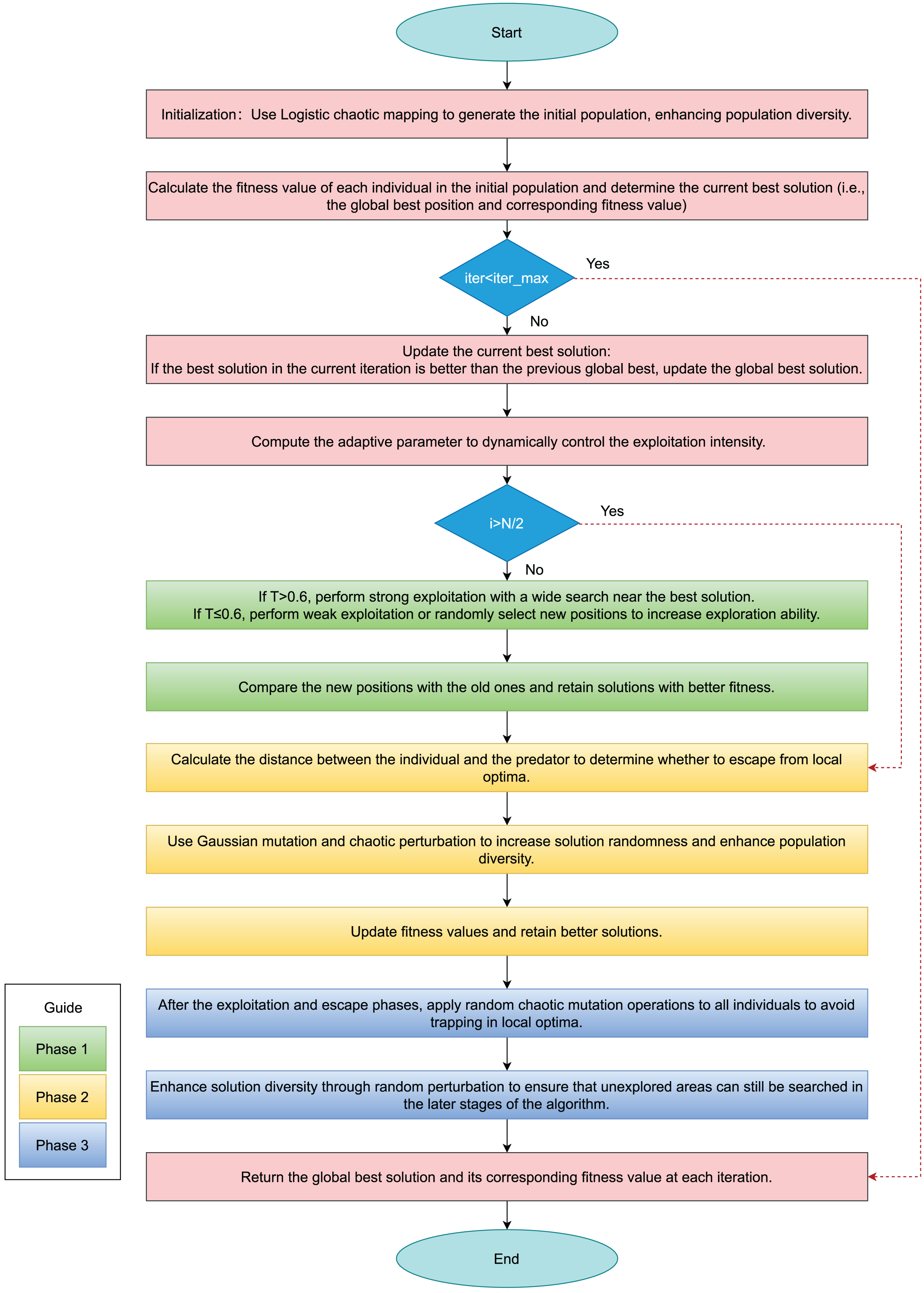
Figure 1 presents the algorithmic flowchart of the improved hippopotamus optimization algorithm, while Algorithm 2 provides the pseudocode for the enhanced HO.
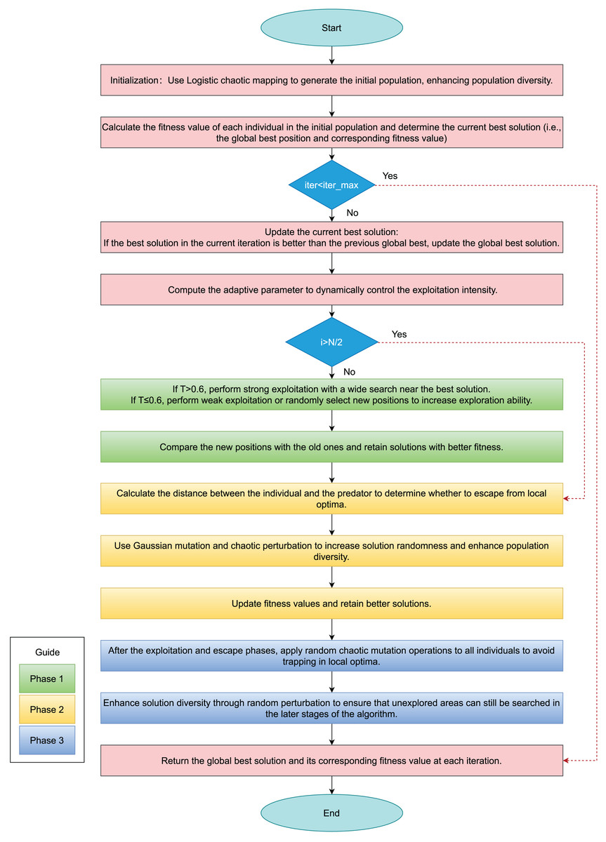
Figure 1: Flowchart of IHO.
| 1: Input: N(SearchAgents), iter_max, lowerbound, upperbound, dimension, fitness |
| 2: Output: best_score, best_pos, IHO_curve |
| 3: Initialize X using the Eq. (10) within bounds |
| 4: Calculate fitness of each agent |
| 5: Set elite as the best solution found |
| 6: for t = 1 to iter_max do |
| 7: Update inertia weight using the Eq. (11) |
| 8: Update mutation rate using the Eq. (14) |
| 9: Step 1: River or Pond (Exploration Phase) |
| 10: for i = 1 to N/2 do |
| 11: Update Dominant_hippopotamus = best solution |
| 12: Compute new positions and using the Eqs. (12), (15), (16) and (3) |
| 13: if fitness( ) is better than current fitness then |
| 14: Update agent’s position to |
| 15: end if |
| 16: if fitness( ) is better than current fitness then |
| 17: Update agent’s position to |
| 18: end if |
| 19: end for |
| 20: Step 2: Defend against Predators (Exploration Phase) |
| 21: for i = N/2 + 1 to N do |
| 22: Generate random predator position |
| 23: Compute new position using the Eq. (8) |
| 24: if fitness( ) is better than current fitness then |
| 25: Update agent’s position to |
| 26: end if |
| 27: end for |
| 28: Step 3: Escape from Predators (Exploitation Phase) |
| 29: for i = 1 to N do |
| 30: Update local boundaries lblocal, ublocal |
| 31: Compute new position using the Eq. (13) |
| 32: if fitness( ) is better than current fitness then |
| 33: Update agent’s position to |
| 34: end if |
| 35: end for |
| 36: Record best solution found in current iteration |
| 37: end for |
| 38: Return the best solution found |
In the Fig. 1, green rectangles represent Phase 1, the adaptive exploitation phase; yellow rectangles indicate Phase 2, the defense phase; and blue rectangles denote Phase 3, the escape phase.
Experiment and analysis
Experimental setup: benchmark functions and parameter configuration
In this study, we compared the effectiveness of the improved IHO with nine classical metaheuristic algorithms, including HO, PSO, sine cosine algorithm (SCA), firefly algorithm (FA), TLBO, Evolution Strategy with Covariance Matrix Adaptation (CMA-ES), moth flame optimization (MFO), arithmetic optimization algorithm (AOA), Invasive Weed Optimization (IWO), Improved Sand Cat Swarm Optimization (ISCSO), penguin jump algorithm (PGJA) and WOA. The control parameters for these algorithms were carefully adjusted according to the specific descriptions provided in Table 1. This section presents the simulation studies of IHO on various complex optimization problems. The effectiveness of IHO in obtaining optimal solutions was evaluated through a comprehensive set of 68 standard benchmark functions. These benchmark functions include unconstrained problems, high-dimensional problems, multi-modal problems and engineering optimization problems. To further evaluate the performance of the algorithms on F1 to F23 (CEC05), 30 independent runs were performed, evaluate the performance of the algorithms on F1 to F30 (CEC17), 50 independent runs were performed, evaluate the performance of the algorithms on F1 to F12 (CEC22), 50 independent runs were performed, evaluate the performance of the algorithms on engineering optimization problems, 30 independent runs were performed. The population size for IHO was set to 24 members in AOA and TLBO, while other algorithms used 30 or 60 members, with the maximum number of iterations set to 1,000 on CEC05. The optimization results are presented using five comprehensive statistical metrics: mean, best, worst, standard deviation, and median. Among these, the mean index was particularly used as a key ranking parameter to evaluate the effectiveness of the metaheuristic algorithms on each benchmark function.
| Algorithm | Parameter | Value |
|---|---|---|
| HO | Search agents | 24 |
| PSO | Velocity limit | 10% of dimension range |
| Cognitive and social constant | (C1, C2) = (2, 2) | |
| Topology | Fully connected | |
| Inertia weight | Linear reduction from 0.9 to 0.1 | |
| SCA | A | 2 |
| FA | Alpha ( ) | 0.2 |
| Beta ( ) | 1 | |
| Gamma ( ) | 1 | |
| TLBO | Teaching factor (TF) | round(1+rand) |
| Rand | A random number between 0 and 1 | |
| CMA-ES | (0) | 0.5 |
| MFO | b | 1 |
| r | Linear reduction −1 to −2 | |
| AOA | a | 0 |
| 0.5 | ||
| IWO | Minimum number of seeds (Smin) | 0 |
| Maximum number of seeds (Smax) | 5 | |
| Initial value of standard deviation | 1 | |
| Final value of standard deviation | 0.001 | |
| Variance reduction exponent | 2 |
This study evaluated 23 functions (CEC05), among which F1–F7 are unimodal (UM) functions, F8–F13 are high-dimensional multimodal (HM) functions, and F14–F23 include fixed-dimensional multimodal (FM) and multimodal (MM) functions.
Specifically, the simulation environment was as follows: Windows 10, Intel Xeon CPU E5-1660 3.0 GHz, 128 GB memory.
Algorithm performance comparison
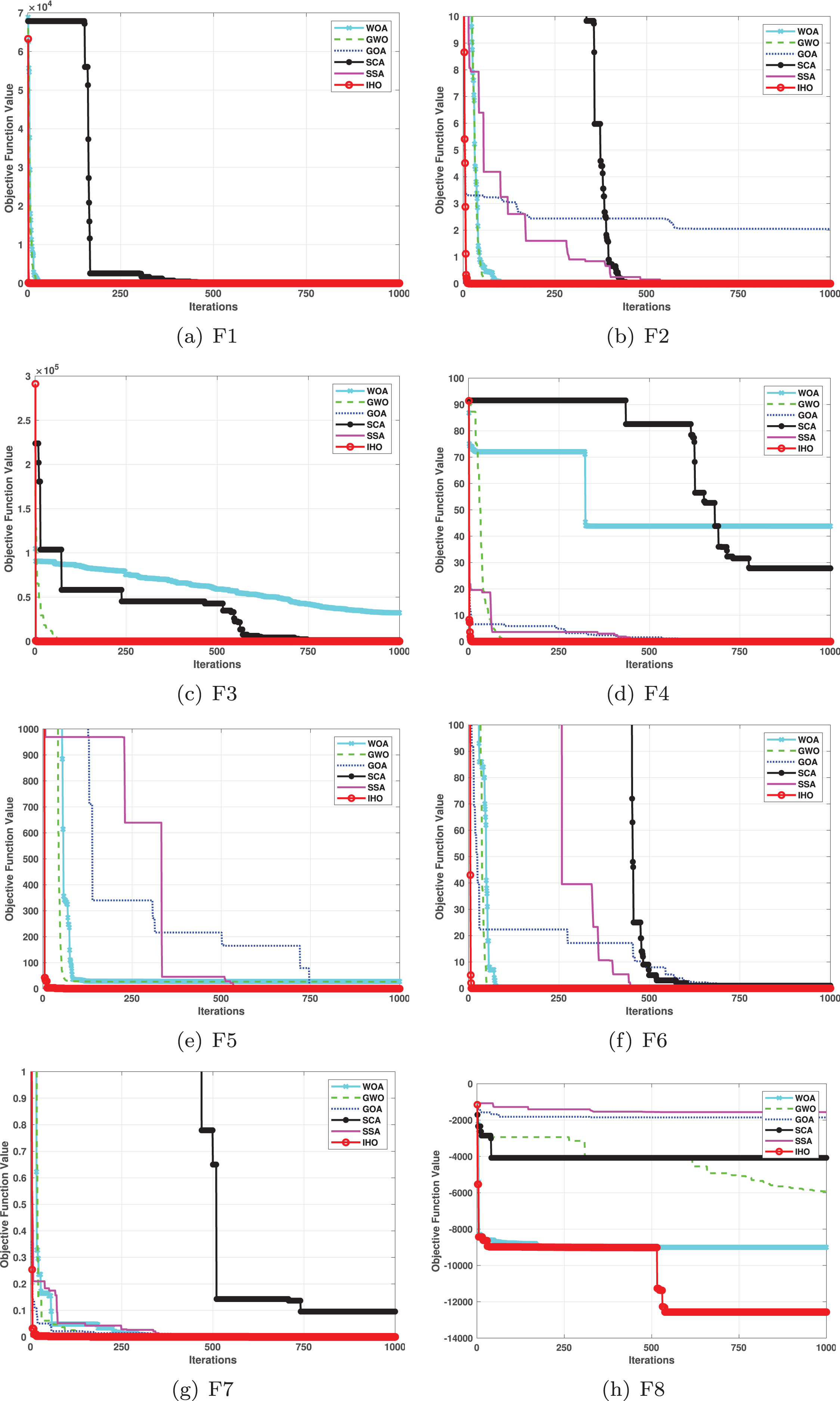
This section provides a detailed comparison of the performance of IHO against the standard HO and other widely used algorithms. The experimental results demonstrate the superior performance of IHO in terms of solution accuracy, convergence speed, and global search capability, particularly for multi-modal functions. Tables 2–4 shows the evaluation results of the benchmark functions, while Figs. 2–4 illustrates the convergence behavior of the five most effective algorithms when optimizing F1–F23 (CEC05).
| F | M | IHO | HO | PSO | SCA | FA | TLBO | CMA-ES | MFO | AOA | IWO |
|---|---|---|---|---|---|---|---|---|---|---|---|
| F1 | Mean | 0 | 0 | 3.69E−06 | 14.855 | 9,712.8 | 1.24E−89 | 3.2243E−08 | 672.36 | 9.07E−13 | 1,292.5 |
| Best | 0 | 0 | 1.11E−07 | 0.12079 | 2,686.8 | 1.95E−91 | 1.5314E−08 | 0.71101 | 4.77E−160 | 3.4203 | |
| Worst | 0 | 0 | 6.65E−05 | 77.5 | 15.976 | 7.75E−89 | 7.6176E−08 | 10,009 | 2.72E−11 | 4,731.2 | |
| Std | 0 | 0 | 1.19E−05 | 20.848 | 2,903 | 1.55E−89 | 1.36E−08 | 2,536.9 | 4.97E−12 | 1,101.6 | |
| Median | 0 | 0 | 7.37E−07 | 4.6546 | 9,605.9 | 7.33E−90 | 3.1564E−08 | 2.7663 | 3.04E−81 | 1,019.3 | |
| F2 | Mean | 0 | 0 | 0.0034028 | 0.13089 | 796.13 | 4.19E-45 | 0.00025096 | 27.865 | 7.60E−209 | 0.10835 |
| Best | 0 | 0 | 6.72E−05 | 0.00023745 | 5.1074 | 2.42E-46 | 0.00013828 | 0.11195 | 1.88E−259 | 0.04844 | |
| Worst | 0 | 0 | 0.049467 | 0.070743 | 19,630 | 1.15E-44 | 0.0004223 | 80.013 | 2.28E−207 | 0.19307 | |
| Std | 0 | 0 | 0.0091893 | 0.017935 | 3,561.4 | 3.09E−45 | 7.04E−05 | 21.195 | 0 | 0.033356 | |
| Median | 0 | 0 | 0.000676 | 0.0048081 | 118.56 | 3.40E−45 | 0.00025537 | 25.302 | 1.36E−233 | 0.10201 | |
| F3 | Mean | 0 | 0 | 162.1 | 7,903.2 | 17,097 | 5.07E−18 | 0.023561 | 19,119 | 0.0075389 | 9,501.9 |
| Best | 0 | 0 | 36.17 | 224.73 | 7,098.1 | 6.80E−21 | 0.0023696 | 3,189.6 | 2.59E−126 | 2,067.5 | |
| Worst | 0 | 0 | 399.71 | 24,159 | 28,712 | 9.53E−17 | 0.090665 | 42,334 | 0.047224 | 25,025 | |
| Std | 0 | 0 | 89.026 | 5,848.9 | 4,911.1 | 1.72E−17 | 0.023315 | 10,697 | 0.011884 | 4,795.7 | |
| Median | 0 | 0 | 154.08 | 6,901.6 | 16,339 | 1.20E−18 | 0.015358 | 19,243 | 3.59E−12 | 8,431.1 | |
| F4 | Mean | 0 | 1.43E−217 | 2.828 | 35.686 | 42.732 | 1.30E−36 | 0.0020537 | 67.677 | 0.027967 | 37.301 |
| Best | 0 | 9.84E−255 | 0.97132 | 13.438 | 28.564 | 1.24E−37 | 0.0010508 | 49.754 | 9.60E−54 | 26.965 | |
| Worst | 0 | 3.01E−216 | 6.9104 | 64.384 | 51.977 | 5.75E−36 | 0.0039077 | 83.333 | 0.046479 | 50.889 | |
| Std | 0 | 0 | 1.3593 | 12.293 | 6.0607 | 1.35E−36 | 0.0061183 | 9.6399 | 0.019333 | 5.2665 | |
| Median | 0 | 4.02E−233 | 2.4615 | 33.964 | 43.963 | 8.93E−37 | 0.0018613 | 69.183 | 0.040356 | 38.063 | |
| F5 | Mean | 0.021681 | 0.12111 | 43.819 | 53,121 | 8,585.4 | 25.425 | 56.719 | 2.68E+06 | 28.5 | 145.47 |
| Best | 0.000006 | 0 | 5.8924 | 43.934 | 30.427 | 24.579 | 20.528 | 185.69 | 27.613 | 23.25 | |
| Worst | 0.157879 | 1.9637 | 119.87 | 3.25E+05 | 41,425 | 26.293 | 684.86 | 8.00E+07 | 28.916 | 1,692.8 | |
| Std | 3.565701E−02 | 0.36433 | 33.794 | 92,441 | 11,144 | 0.39027 | 127.83 | 1.46E+07 | 0.29675 | 314.02 | |
| Median | 0.004886 | 0.0070966 | 25.626 | 6,262.6 | 3,219 | 25.42 | 22.307 | 880.08 | 28.522 | 29.201 | |
| F6 | Mean | 0 | 0 | 4.5 | 17.067 | 21,561 | 0 | 0 | 1,727.8 | 0 | 3,023.2 |
| Best | 0 | 0 | 0 | 0 | 9,654 | 0 | 0 | 1 | 0 | 502 | |
| Worst | 0 | 0 | 37 | 139 | 28,728 | 0 | 0 | 10,225 | 0 | 6,159 | |
| Std | 0 | 0 | 7.2099 | 31.139 | 4,301 | 0 | 0 | 3,791.4 | 0 | 1,649.4 | |
| Median | 0 | 0 | 1.5 | 6 | 22,142 | 0 | 0 | 13.5 | 0 | 2,818.5 | |
| F7 | Mean | 6.436959E−05 | 3.54E−05 | 0.024313 | 0.1112 | 0.076687 | 0.0011331 | 0.011562 | 4.3902 | 5.80E−05 | 0.071947 |
| Best | 2.084746E−06 | 1.30E−06 | 0.0094839 | 0.018044 | 0.035773 | 0.0004299 | 0.005156 | 0.065606 | 1.76E−06 | 0.029085 | |
| Worst | 1.975755E−04 | 0.00013102 | 0.055549 | 0.89506 | 0.15281 | 0.0023231 | 0.017513 | 77.983 | 0.00033704 | 0.12335 | |
| Std | 5.211867E−05 | 4.10E−05 | 0.011822 | 0.16168 | 0.029595 | 0.00050432 | 0.0032379 | 14.338 | 7.42E−05 | 0.020096 | |
| Median | 4.521877E−05 | 1.99E−05 | 0.020326 | 0.064266 | 0.073503 | 0.0009457 | 0.012149 | 0.28247 | 2.67E−05 | 0.070357 | |
| F8 | Mean | −13,073.468434 | −12,567 | −6,590.1 | −3,734.5 | −7,463.7 | −7,906.9 | −4,363.9 | −8,496.8 | −5,340.9 | −6,695.5 |
| Best | −20,290.596194 | −12,569 | −8,325.1 | −4,553.8 | −8,678.6 | −9,427.3 | −5,177.9 | −9,778.5− | 6,242.2 | −8,233.1 | |
| Worst | −12,569.404004 | −12,530 | −4,337.3 | −3,362.8 | −6,488.8 | −5,915.7 | −3,860.7 | −6,725.5 | −4,587.8 | −4,759.4 | |
| Std | 1.918477E+03 | 7.3469 | 903.25 | 281.89 | 615.82 | 781.93 | 320.79 | 863.55 | 471.37 | 677.46 | |
| Median | −12,569.483846 | −12,569 | −6,489.3 | −3,679.7 | −7,454.6 | −8,000.2 | −4,301.5 | −8,559.5 | −5,136.7 | −6,646.7 |
| F | M | IHO | HO | PSO | SCA | FA | TLBO | CMA-ES | MFO | AOA | IWO |
|---|---|---|---|---|---|---|---|---|---|---|---|
| F9 | Mean | 0 | 0 | 45.735 | 50.849 | 186.92 | 12.924 | 126.97 | 155.49 | 0 | 65.852 |
| Best | 0 | 0 | 22.884 | 0.03564 | 117.41 | 0 | 6.9667 | 84.588 | 0 | 43.819 | |
| Worst | 0 | 0 | 78.602 | 202.58 | 258.69 | 23.007 | 187.18 | 228.14 | 0 | 93.563 | |
| Std | 0 | 0 | 14.675 | 48.636 | 33.884 | 6.0126 | 71.067 | 40.991 | 0 | 12.894 | |
| Median | 0 | 0 | 45.271 | 38.413 | 187.05 | 13.042 | 162.64 | 152.47 | 0 | 64.752 | |
| F10 | Mean | 4.44E−16 | 4.44E−16 | 1.1408 | 14.229 | 18.297 | 9.21E−15 | 5.6832−05 | 13.321 | 4.44E−16 | 10.679 |
| Best | 4.44E−16 | 4.44E−16 | 6.26E−05 | 0.050121 | 18.271 | 4.00E−15 | 3.4412E−05 | 0.68917 | 4.44E−16 | 0.0087287 | |
| Worst | 4.44E−16 | 4.44E−16 | 2.4083 | 20.402 | 19.296 | 1.03E−13 | 9.5468E−05 | 19.962 | 4.44E−16 | 19.228 | |
| Std | 0 | 0 | 0.82655 | 8.6665 | 0.21681 | 1.79E−14 | 1.5424E−05 | 7.836 | 0 | 9.4921 | |
| Median | 4.44E−16 | 4.44E−16 | 1.3404 | 20.204 | 19.028 | 7.55E−15 | 5.4007E−05 | 17.837 | 4.44E−16 | 18.181 | |
| F11 | Mean | 0 | 0 | 0.021824 | 0.91439 | 163.94 | 0 | 2.9979e−07 | 6.9724 | 0.1554 | 480.41 |
| Best | 0 | 0 | 4.46E−07 | 0.025341 | 71.221 | 0 | 8.804E−08 | 0.43489 | 0.00044758 | 333.51 | |
| Worst | 0 | 0 | 0.087692 | 1.6975 | 237.77 | 0 | 7.7197E−07 | 91.085 | 0.43829 | 640.31 | |
| Std | 0 | 0 | 0.026358 | 0.42847 | 36.504 | 0 | 1.7512e−07 | 22.846 | 0.11095 | 71.029 | |
| Median | 0 | 0 | 0.0098613 | 0.99061 | 163.4 | 0 | 2.6344E−07 | 1.0093 | 0.13784 | 477.65 | |
| F12 | Mean | 0.000132 | 9.3E−09 | 0.11094 | 40,328 | 42.51 | 0.0034654 | 1.9945E−09 | 17.719 | 0.51896 | 8.8769 |
| Best | 0 | 1.49E−09 | 6.84E−09 | 0.79446 | 13.932 | 6.74E−09 | 7.8685E−10 | 0.70708 | 0.41734 | 3.4841 | |
| Worst | 0.000610 | 7.32E−08 | 1.0405 | 7.11E+05 | 76.246 | 0.10367 | 7.2421E−09 | 285.16 | 0.61102 | 12.625 | |
| Std | 2.203374E−04 | 1.62E−08 | 0.23009 | 1.47E+05 | 15.885 | 0.0118926 | 1.3528E−09 | 50.987 | 0.050388 | 1.8974 | |
| Median | 0.000011 | 5.33E−09 | 2.09E−05 | 17.858 | 44.103 | 1.14E−07 | 1.6197E−09 | 6.8694 | 0.527 | 8.9038 | |
| F13 | Mean | 0.003340 | 0.0050467 | 0.021928 | 6.69E+05 | 44,205 | 0.072491 | 2.128E−08 | 2.731E+07 | 2.81 | 0.0027154 |
| Best | 0 | 1.35E−32 | 1.03E−08 | 2.7393 | 50.302 | 2.23E−06 | 7.311E−09 | 2.1321 | 2.6101 | 5.00E−05 | |
| Worst | 0.019808 | 0.063492 | 0.28572 | 1.31E+07 | 3.97E+05 | 0.20724 | 4.3763E−08 | 4.10E+08 | 2.9944 | 0.011275 | |
| Std | 5.546983E−03 | 0.012164 | 0.05445 | 2.56e+06 | 86.550 | 0.069667 | 9.3747E−09 | 1.04E+08 | 0.092163 | 0.0047482 | |
| Median | 0.000143 | 0.0014522 | 0.010988 | 1,130.3 | 2,772.3 | 0.047853 | 1.9344E−08 | 29.131 | 2.7955 | 0.00014517 | |
| F14 | Mean | 0.998004 | 0.998 | 5.5195 | 2.2512 | 9.502 | 0.998 | 4.7816 | 2.51 | 8.0876 | 11.358 |
| Best | 0.998004 | 0.998 | 0.998 | 0.998 | 0.998 | 0.998 | 1.992 | 0.998 | 0.998 | 0.998 | |
| Worst | 0.998004 | 0.998 | 12.671 | 10.763 | 21.988 | 0.998 | 11.721 | 10.763 | 12.671 | 23.809 | |
| Std | 0 | 0 | 3.0682 | 1.8878 | 6.2553 | 3.86E−16 | 2.4391 | 2.3156 | 4.7721 | 7.3331 | |
| Median | 0.998004 | 0.998 | 5.9288 | 2.0092 | 8.3574 | 0.998 | 3.9742 | 0.998 | 10.763 | 10.763 | |
| F15 | Mean | 0.000308 | 0.00030836 | 0.0024923 | 0.0010454 | 0.0058617 | 0.00036839 | 0.0019 | 0.0013293 | 0.0071685 | 0.0027859 |
| Best | 0.000307 | 0.00030749 | 0.00030749 | 0.00057375 | 0.00030749 | 0.00030749 | 0.0011 | 0.000742582 | 0.00034241 | 0.00058505 | |
| Worst | 0.000308 | 0.00031288 | 0.020363 | 0.0016389 | 0.020363 | 0.0012232 | 0.0035 | 0.0083337 | 0.069975 | 0.020363 | |
| Std | 4.603049E−08 | 1.31E−06 | 0.0060732 | 0.00035949 | 0.089054 | 0.00018223 | 7.25E−06 | 0.0013978 | 0.014639 | 0.0059637 | |
| Median | 0.000307 | 0.00030779 | 0.00030782 | 0.00087851 | 0.00030749 | 0.00030749 | 0.0016 | 0.00080207 | 0.00047392 | 0.00074539 | |
| F16 | Mean | −1.031628 | −1.0316 | −1.0316 | −1.0316 | −0.8956 | −1.0316 | −1.0316 | −1.0316 | −1.0316 | −1.0316 |
| Best | −1.031628 | −1.0316 | −1.0316 | −1.0316 | −1.0316 | −1.0316 | −1.0316 | −1.0316 | −1.0316 | −1.0316 | |
| Worst | −1.031628 | −1.0316 | −1.0316 | −1.0314 | −0.21543 | −1.0316 | −1.0316 | −1.0316 | −1.0316 | −1.0316 | |
| Std | 5.258941E−13 | 5.96E−16 | 6.71E-16 | 5.7E-05 | 0.30937 | 6.65E-16 | 6.78E−16 | 6.78E−16 | 1.22E−16 | 1.44E−08 | |
| Median | −1.031628 | −1.0316 | −1.0316 | −1.0316 | −1.0316 | −1.0316 | −1.0316 | −1.0316 | −1.0316 | −1.0316 |
| F | M | IHO | HO | PSO | SCA | FA | TLBO | CMA-ES | MFO | AOA | IWO |
|---|---|---|---|---|---|---|---|---|---|---|---|
| F17 | Mean | 0.397887 | 0.39789 | 0.39789 | 0.40008 | 0.39789 | 0.39789 | 0.39789 | 0.39789 | 0.41197 | 0.39789 |
| Best | 0.39789 | 0.39789 | 0.39789 | 0. 3,979 | 0.39789 | 0.39789 | 0.39789 | 0. 39,789 | 0.39813 | 0.39789 | |
| Worst | 0.397887 | 0.39789 | 0.39789 | 0.40747 | 0.39789 | 0.39789 | 0.39789 | 0.39789 | 0. 4415 | 0.39789 | |
| Std | 0 | 0 | 7.23E−16 | 0.0023394 | 3.86E−11 | 0 | 0 | 0 | 0.01286 | 5.57E−09 | |
| Median | 0.397887 | 0.39789 | 0.39789 | 0.39939 | 0.39789 | 0. 39789 | 0.39789 | 0.39789 | 0.40712 | 0.39789 | |
| F18 | Mean | 3 | 3 | 3.9 | 3.0001 | 3.9 | 3 | 3 | 3 | 7.7674 | 3 |
| Best | 3 | 3 | 3 | 3 | 3 | 3 | 3 | 3 | 3 | 3 | |
| Worst | 3 | 3 | 30 | 3.0004 | 30 | 3 | 3 | 3 | 37.986 | 3 | |
| Std | 2.365956E−11 | 1.27E−15 | 4.9295 | 0.00010081 | 4.9295 | 5.53E−16 | 1.35E−15 | 1.62E−15 | 10.92 | 8.47E−07 | |
| Median | 3 | 3 | 3 | 3 | 3 | 3 | 3 | 3 | 3 | 3 | |
| F19 | Mean | −3.862782 | −3.8628 | −3.8628 | −3.8542 | −3.8628 | −3.8628 | −3.8628 | −3.8628 | −3.8512 | −3.8628 |
| Best | −3.862782 | −3.8628 | −3.8628 | −3.8621 | −3.8628 | −3.8628 | −3.8628 | −3.8628 | −3.8605 | −3.8628 | |
| Worst | −3.862782 | −3.8628 | −3.8628 | −3.8443 | −3.8628 | −3.8628 | −3.8628 | −3.8628 | −3.8408 | −3.8628 | |
| Std | 6.386724E−09 | 2.70E−15 | 6.42E−07 | 0.0032649 | 5.72E−11 | 2.71E−15 | 2.71E−15 | 2.71E−15 | 0.0088724 | 6.32E−07 | |
| Median | −3.862782 | −3.8628 | −3.8628 | −3.8542 | −3.8628 | −3.8628 | −3.8628 | −3.8628 | −3.8516 | −3.8628 | |
| F20 | Mean | −3.300409 | −3.322 | −3.2784 | −2.8823 | −3.2586 | −3.2811 | −3.2919 | −3.2422 | −3.0755 | −3.203 |
| Best | −3.321995 | −3.322 | −3.322 | −3.1473 | −3.322 | −3.3206 | −3.322 | −3.322 | −3.1844 | −3.2031 | |
| Worst | −3.188840 | −3.322 | −3.2031 | −1.9133 | −3.2031 | −3.1059 | −3.2031 | −3.1376 | −2.9507 | −3.2026 | |
| Std | 5.843069E−02 | 9.78E−12 | 0.058273 | 0.32598 | 0.060328 | 0.066162 | 0.051459 | 0.063837 | 0.063759 | 0.00012908 | |
| Median | −3.321995 | −3.322 | −3.322 | −2.9914 | −3.2031 | −3.3109 | −3.322 | −3.2031 | −3.0905 | −3.2031 | |
| F21 | Mean | −10.153200 | −10.153 | −6.3165 | −2.1516 | −5.6345 | −9.778 | −7.9121 | −6.3132 | −3.4351 | −6.6391 |
| Best | −10.153200 | −10.153 | −10.153 | −6.0051 | −10.153 | −10.153 | −10.153 | −10.153 | −5.5613 | −10.153 | |
| Worst | −10.153200 | −10.153 | −2.6305 | −0.35136 | −2.6305 | −3.9961 | −2.6829 | −2.6305 | −1.9507 | −2.6305 | |
| Std | 8.791181E−08 | 4.74E−06 | 3.6985 | 1.872 | 3.1766 | 1.4345 | 3.4819 | 3.5169 | 0.97125 | 3.4561 | |
| Median | −10.153200 | −10.153 | −5.078 | −0.88031 | −5.0552 | −10.153 | −10.153 | −5.078 | −3.2531 | −5.1008 | |
| F22 | Mean | −10.402941 | −10.403 | −6.7572 | −2.7098 | −5.3848 | −9.7414 | −10.403 | −8.2382 | −3.7002 | −7.4415 |
| Best | −10.402941 | −10.403 | −10.403 | −6.3217 | −10.403 | −10.403 | −10.403 | −10.403 | −6.8593 | −10.403 | |
| Worst | −10.402940 | −10.403 | −1.8376 | −0.52104 | −1.8376 | −5.0265 | −10.403 | −2.7519 | −1.2708 | −1.8376 | |
| Std | 5.043988E−08 | 6.16E−05 | 3.7466 | 1.9244 | 3.194 | 1.7896 | 1.65E−15 | 3.3738 | 1.2624 | 3.7449 | |
| Median | −10.402941 | −10.403 | −7.7659 | −2.6079 | −3.7243 | −10.403 | −10.403 | −10.403 | −3.6181 | −10.403 | |
| F23 | Mean | −10.536410 | −10.536 | −6.0645 | −4.1564 | −4.7569 | −10.123 | −10.536 | −7.9819 | −4.6738 | −8.3548 |
| Best | −10.536410 | −10.536 | −10.536 | −8.3393 | −10.536 | −10.536 | −10.536 | −10.536 | −8.6767 | −10.536 | |
| Worst | −10.536409 | −10.536 | −1.8595 | −0.94428 | −1.6766 | −3.8354 | −10.536 | −2.4217 | −1.8573 | −2.4217 | |
| Std | 7.476629E−08 | 2.99E−05 | 3.7424 | 1.5765 | 3.0762 | 1.5801 | 1.78E-15 | 3.6868 | 1.5405 | 3.437 | |
| Median | −10.536410 | −10.536 | −3.8354 | −4.6344 | −3.8354 | −10.536 | −10.536 | −10.536 | −4.8892 | −10.536 |
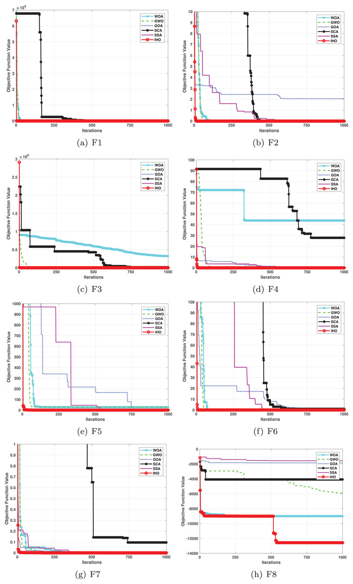
Figure 2: Convergence curves of five algorithms in each benchmark functions (CEC05, F1–F8).
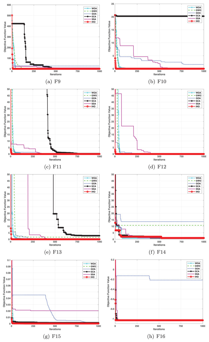
Figure 3: Convergence curves of five algorithms in each benchmark functions (CEC05, F9–F16).
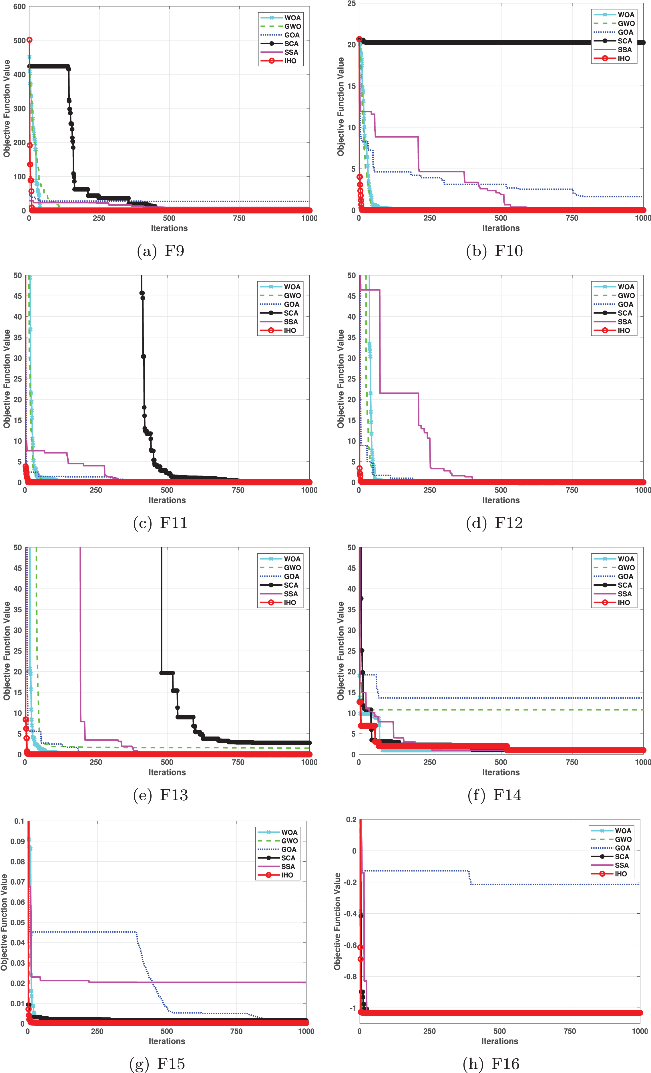
Figure 4: Convergence curves of five algorithms in each benchmark functions (CEC05, F17–F23).
Figures 2–4 illustrates the convergence curves of the five most effective algorithms during the optimization process for F1–F23. This evaluation, as presented in Table 2, aims to assess the algorithms’ local search capabilities on eight distinct unimodal functions (F1–F8). IHO achieved global optima on F1–F4 and F5–F6, making it the only algorithm among the nine evaluated to reach this level of performance. Its performance on F4 significantly surpassed that of the other algorithms. In the highly competitive F6 test, IHO reached global optima alongside four other algorithms. Additionally, IHO demonstrated clear superiority on F7 and F8. For F1–F4 and F6, IHO consistently converged with a standard deviation of zero. For F7, the standard deviation was 5.21E−05, and for F5, it was 3.57E−2. Compared to the other algorithms, IHO exhibited the lowest standard deviation, indicating remarkable stability.
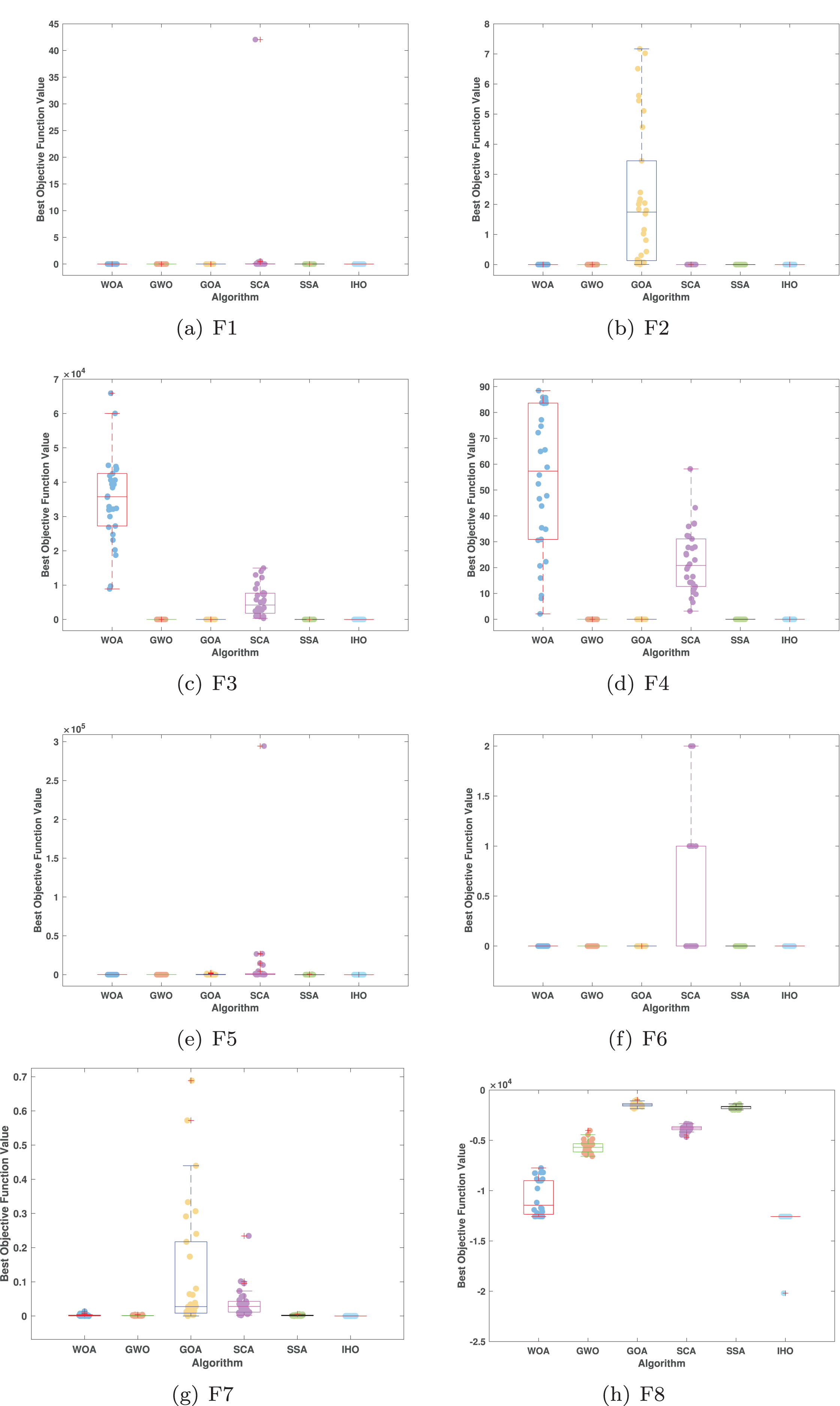
Figures 5–7 displays the box plots of the optimal values of the objective function obtained from 30 independent runs on F1–F23 (CEC05), utilizing IHO and five other algorithms.
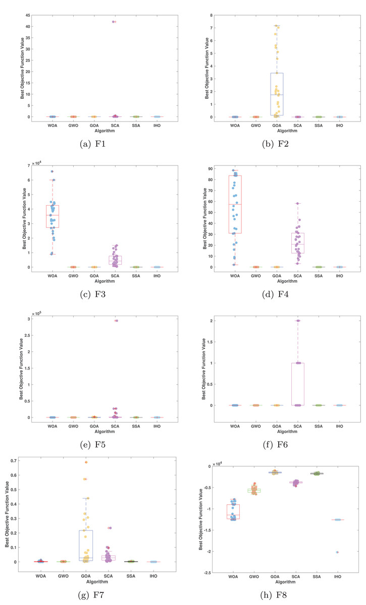
Figure 5: Boxplot illustrating the performance of the IHO in comparison to other algorithms (CEC05, F1–F8).
Figure 6: Boxplot illustrating the performance of the IHO in comparison to other algorithms (CEC05, F9–F16).
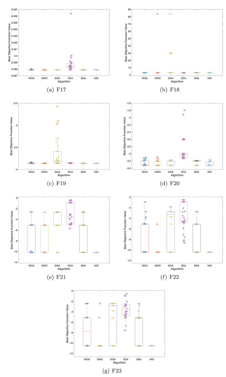
Figure 7: Boxplot illustrating the performance of the IHO in comparison to other algorithms (CEC05, F17–F23).
Table 3 presents the results for HM functions on F9–F16, tested using different algorithms. These functions were chosen to evaluate the global search capabilities of the algorithms. IHO significantly outperformed all other algorithms on F12 and F13. In F9, IHO achieved global optima along with HO and AOA, demonstrating superior performance over the other algorithms. On F10, IHO performed comparably to HO and surpassed all other algorithms. For F11, IHO converged to the global optimum alongside HO and TLBO, showcasing exceptional performance. IHO also outperformed all other algorithms on F12, and in F13, IHO ranked first. In F16, IHO exhibited a notably lower standard deviation than some algorithms. For F13, the standard deviation was 5.55E−3, outperforming all other algorithms. These findings indicate that IHO demonstrates robust resilience in effectively handling these functions (refer to Fig. 3).
Furthermore, an assessment was conducted to examine the algorithm’s ability to balance exploration and exploitation during searches on F17–F23, with results recorded in Table 4. IHO exhibited the best performance on F17–F23, achieving a significantly lower standard deviation, particularly for F21–F23. These results suggest that IHO, characterized by a strong capacity to balance exploration and exploitation, exhibits outstanding performance when addressing FM and MM functions.
In benchmarked tests for CEC17 and CEC22, IHO was compared against four algorithms, including ISCSO, PGJA, SCA, and WOA. We run each problem 51 times independently. Comparison results between IHO and other algorithms are shown in Tables 5 to 15.
| F | M | ISCSO | PGJA | SCA | WOA | IHO |
|---|---|---|---|---|---|---|
| F1 | Mean | 4,987.123315 | 5,152,068,207 | 453,892,150.8 | 5,677.886088 | 425.3499924 |
| Worst | 7,462.523097 | 14,176,457,086 | 828,619,257.2 | 11,768.29185 | 1,392.986225 | |
| Best | 1,883.922791 | 501,940,941.8 | 224,092,914.3 | 817.6520327 | 109.1973094 | |
| Std | 2,421.895976 | 4,208,212,553 | 193,082,106.7 | 4,795.956709 | 424.9428172 | |
| p-value | 0.0001554 | 0.0001554 | 0.0001554 | 0.0004662 | ||
| F3 | Mean | 300.0048631 | 28,326.28152 | 738.5664608 | 319.5393755 | 300.0000036 |
| Worst | 300.0129943 | 59,965.39757 | 949.3114193 | 387.2733974 | 300.0000039 | |
| Best | 300.0014739 | 12,745.49304 | 578.2110906 | 301.5697167 | 300.0000033 | |
| Std | 0.003786698 | 19,742.95592 | 131.4069608 | 29.43817809 | 2.88E−07 | |
| p-value | 0.0001554 | 0.0001554 | 0.0001554 | 0.0001554 | – | |
| F4 | Mean | 401.6984057 | 971.294942 | 424.9710217 | 422.7298603 | 400.0972279 |
| Worst | 402.4788786 | 1,634.217658 | 432.602983 | 480.1877739 | 400.0972279 | |
| Best | 400.2932751 | 503.0818602 | 418.3269302 | 403.3673956 | 400.0972279 | |
| Std | 0.662455257 | 407.8453014 | 4.84319693 | 31.86833438 | 0 | |
| p-value | 0.0001554 | 0.0001554 | 0.0001554 | 0.0001554 | – | |
| F5 | Mean | 525.4378711 | 578.7101462 | 539.3010021 | 550.4831931 | 531.9629316 |
| Worst | 550.2631156 | 598.1207866 | 551.9366662 | 576.7734447 | 545.7679413 | |
| Best | 512.9352649 | 557.6157058 | 533.0219727 | 522.8844111 | 509.9495863 | |
| Std | 12.03057378 | 16.00161696 | 5.845632604 | 16.77641932 | 5.526872364 | |
| p-value | 0.016472416 | 0.0001554 | 0.211965812 | 0.212587413 | – | |
| F6 | Mean | 615.043237 | 651.3019612 | 613.4589642 | 618.8880448 | 604.5450446 |
| Worst | 623.4759625 | 673.0403356 | 617.8767148 | 631.5962627 | 604.5450446 | |
| Best | 608.4757515 | 629.8806275 | 608.3111776 | 612.0278709 | 601.4792689 | |
| Std | 4.112977893 | 15.36811062 | 3.249770499 | 5.776172275 | 5.170038862 | |
| p-value | 0.0001554 | 0.0001554 | 0.0001554 | 0.0001554 | – | |
| F7 | Mean | 767.696279 | 812.1582608 | 761.6917992 | 769.7738782 | 736.2916253 |
| Worst | 796.9088529 | 835.8907197 | 773.7917762 | 810.7424527 | 730.2916253 | |
| Best | 741.6644502 | 778.5043777 | 752.6181514 | 755.0158719 | 727.9820221 | |
| Std | 18.68517396 | 22.46842876 | 6.516619375 | 20.01406921 | 22.98925146 | |
| p-value | 0.033411033 | 0.0001554 | 0.26993007 | 0.152292152 | – | |
| F8 | Mean | 828.7295445 | 857.8577399 | 827.6090855 | 836.6903697 | 821.267219 |
| Worst | 842.7832089 | 887.0136726 | 842.1572056 | 848.7532071 | 822.8840131 | |
| Best | 814.9246164 | 830.502357 | 820.0987876 | 821.890121 | 815.919331 | |
| Std | 8.826341479 | 19.24227874 | 7.491915403 | 8.66508297 | 4.573016158 | |
| p-value | 0.088578089 | 0.0001554 | 0.425951826 | 0.0003108 | – | |
| F9 | Mean | 1,080.380236 | 1,944.200946 | 940.6257476 | 1,462.3526 | 900 |
| Worst | 1,185.15901 | 2,849.769501 | 1,001.100877 | 3,199.749399 | 900 | |
| Best | 903.5457809 | 1,105.766715 | 916.6051911 | 989.5193139 | 900 | |
| Std | 89.98589908 | 663.2691308 | 29.00918399 | 712.9630477 | 0 | |
| p-value | 0.0001554 | 0.0001554 | 0.0001554 | 0.0001554 | – | |
| F10 | Mean | 1,810.778037 | 2,622.657972 | 2,071.511798 | 1,991.618814 | 1,243.198114 |
| Worst | 1,926.625916 | 3,000.609949 | 2,327.715403 | 2,283.262482 | 1,243.198114 | |
| Best | 1,118.646839 | 2,108.924388 | 1,817.11791 | 1,681.878592 | 1,243.198114 | |
| Std | 282.7225444 | 293.8512235 | 189.8125496 | 187.280999 | 0 | |
| p-value | 0.005749806 | 0.0001554 | 0.0001554 | 0.0001554 | – | |
| F11 | Mean | 1,129.236945 | 2,224.42686 | 1,175.235781 | 1,171.019655 | 1,122.027224 |
| Worst | 1,223.503721 | 4,021.684916 | 1,280.410351 | 1,261.759158 | 1,120.027224 | |
| Best | 1,106.854316 | 1,262.455908 | 1,141.673395 | 1,131.294941 | 1,118.40417 | |
| Std | 39.39308907 | 1,011.358464 | 43.89837056 | 41.65821637 | 5.821715642 | |
| p-value | 0.141258741 | 0.0001554 | 0.0001554 | 0.0001554 | – |
| F | M | ISCSO | PGJA | SCA | WOA | IHO |
|---|---|---|---|---|---|---|
| F12 | Mean | 15,500.44852 | 69,702,386.15 | 5,484,677.173 | 3,733,118.946 | 7,244.032995 |
| Worst | 41,581.17202 | 2,68,355,231.3 | 24,921,041.74 | 11,681,992.88 | 10,332.20899 | |
| Best | 2,420.308225 | 4,639,492.886 | 311,759.8881 | 12,598.27213 | 4,447.057512 | |
| Std | 14,144.74464 | 86,696,374.66 | 7,956,068.409 | 4,566,798.445 | 2,037.535011 | |
| p-value | 0.694327894 | 0.0001554 | 0.0001554 | 0.000621601 | – | |
| F13 | Mean | 6,603.652817 | 2,570,794.312 | 8,964.410908 | 16,017.15392 | 2,761.521945 |
| Worst | 15,486.46427 | 7,741,754.264 | 14,231.06068 | 54,505.33354 | 3,923.922656 | |
| Best | 1,503.173747 | 7,815.113334 | 3,281.696832 | 2,414.126219 | 1,700.251804 | |
| Std | 4,446.803911 | 3,585,718.047 | 3,604.847762 | 18,191.85426 | 874.7351623 | |
| p-value | 0.428127428 | 0.0001554 | 0.007925408 | 0.428127428 | – | |
| F14 | Mean | 1,466.944324 | 1,789.204279 | 1,510.786667 | 1,510.233472 | 1,446.784048 |
| Worst | 1,490.696059 | 1,874.139619 | 1,557.509699 | 1,554.596642 | 1,445.784048 | |
| Best | 1,442.195229 | 1,671.107152 | 1,474.199885 | 1,446.827282 | 1,444.017391 | |
| Std | 17.77802576 | 69.46464676 | 24.15437664 | 35.62557825 | 19.57333086 | |
| p-value | 0.404195804 | 0.0001554 | 0.005749806 | 0.005749806 | – | |
| F15 | Mean | 1,532.435549 | 22,658.0514 | 1,743.927269 | 2,178.805327 | 1,588.391776 |
| Worst | 1,565.068607 | 41,491.91855 | 1,949.778361 | 4,917.587161 | 1,568.391776 | |
| Best | 1,513.721288 | 11,804.87546 | 1,608.456658 | 1,552.217692 | 1,546.496198 | |
| Std | 21.21370731 | 9,807.425367 | 116.2118651 | 1,126.062543 | 46.17100853 | |
| p-value | 0.0001554 | 0.0001554 | 0.045376845 | 0.098212898 | – | |
| F16 | Mean | 1,840.967016 | 2,017.155024 | 1,664.989324 | 1,825.098683 | 1,612.578714 |
| Worst | 1,990.826531 | 2,168.334864 | 1,747.147766 | 1,943.234022 | 1,613.283201 | |
| Best | 1,721.892698 | 1,925.258736 | 1,630.503759 | 1,610.639455 | 1,612.478073 | |
| Std | 107.879074 | 94.71349596 | 35.62449591 | 106.2893587 | 0.284655822 | |
| p-value | 0.305050505 | 0.0001554 | 0.000621601 | 0.008391608 | – | |
| F17 | Mean | 1,758.598857 | 1,887.343989 | 1,762.472079 | 1,754.298622 | 1,742.590785 |
| Worst | 1,767.225638 | 2,028.271588 | 1,777.32652 | 1,772.387575 | 1,751.510034 | |
| Best | 1,742.23283 | 1,777.123288 | 1,756.040438 | 1,746.814912 | 1,727.725372 | |
| Std | 7.995523967 | 89.46217558 | 7.103721377 | 8.39444804 | 12.30973196 | |
| p-value | 0.009479409 | 0.0001554 | 0.0001554 | 0.435120435 | – | |
| F18 | Mean | 19,232.70015 | 2,476,478.355 | 58,435.879 | 19,803.47944 | 2,043.094365 |
| Worst | 45,227.44588 | 15,500,448.49 | 121,581.7599 | 38,859.26493 | 2,168.551001 | |
| Best | 3,062.104297 | 11,679.04117 | 33,396.40452 | 2,330.88776 | 1,895.261609 | |
| Std | 13,524.12215 | 5,341,003.63 | 29,629.35695 | 13,202.58429 | 392.1042637 | |
| p-value | 0.0001554 | 0.0001554 | 0.0001554 | 0.0001554 | – | |
| F19 | Mean | 1,923.901044 | 28,665.59854 | 2,114.878879 | 26,955.70709 | 1,940.65217 |
| Worst | 1,931.891439 | 104,706.9098 | 2,276.780707 | 112,795.7633 | 1,990.856998 | |
| Best | 1,914.481335 | 2,038.567496 | 1,976.507273 | 2,759.738166 | 1,906.403849 | |
| Std | 6.243335105 | 32,000.17485 | 101.2430295 | 36,743.23508 | 28.30599937 | |
| p-value | 0.0001554 | 0.0001554 | 0.0001554 | 0.0001554 | – | |
| F20 | Mean | 2,158.864646 | 2,207.448872 | 2,065.34018 | 2,126.241696 | 2,047.081574 |
| Worst | 2,236.338875 | 2,295.259967 | 2,098.766204 | 2,205.176509 | 2,050.141926 | |
| Best | 2,039.529609 | 2,076.860971 | 2,036.44419 | 2,051.716088 | 2,035.988619 | |
| Std | 67.24935225 | 61.73073421 | 17.07862108 | 60.64364337 | 60.45100662 | |
| p-value | 0.083139083 | 0.005749806 | 0.005749806 | 0.404195804 | – | |
| F21 | Mean | 2,200.757078 | 2,307.476403 | 2,207.374272 | 2,270.419438 | 2,223.684384 |
| Worst | 2,203.598813 | 2,384.143801 | 2,210.342896 | 2,345.950974 | 2,294.737522 | |
| Best | 2,200.003631 | 2,226.252765 | 2,203.282162 | 2,204.46207 | 2,200.000005 | |
| Std | 1.221212601 | 61.31568217 | 2.340995504 | 66.44060791 | 43.85494879 | |
| p-value | 0.093706294 | 0.003418803 | 0.093706294 | 0.008547009 | – |
| F | M | ISCSO | PGJA | SCA | WOA | IHO |
|---|---|---|---|---|---|---|
| F22 | Mean | 2,332.246804 | 2,631.769368 | 2,322.340101 | 2,372.951026 | 2,291.536988 |
| Worst | 2,406.281485 | 3,257.792962 | 2,343.626277 | 2,757.41482 | 2,305.072932 | |
| Best | 2,308.422587 | 2,327.533254 | 2,279.142406 | 2,309.960526 | 2,212.847318 | |
| Std | 32.40782935 | 284.1795227 | 25.13327707 | 155.4368648 | 31.81831746 | |
| p-value | 0.0001554 | 0.0001554 | 0.088578089 | 0.0001554 | – | |
| F23 | Mean | 2,641.068178 | 2,682.44855 | 2,649.297214 | 2,644.496033 | 2,606.826544 |
| Worst | 2,653.366621 | 2,722.826597 | 2,653.906069 | 2,664.430431 | 2,606.826544 | |
| Best | 2,626.797346 | 2,638.175271 | 2,646.622882 | 2,620.958212 | 2,606.826544 | |
| Std | 9.498932884 | 30.61273839 | 2.388264412 | 15.90551062 | 0 | |
| p-value | 0.0001554 | 0.0001554 | 0.0001554 | 0.0001554 | – | |
| F24 | Mean | 2,500.061424 | 2,800.353532 | 2,775.398787 | 2,778.338253 | 2,628.802761 |
| Worst | 2,500.092632 | 2,829.524799 | 2,783.262573 | 2,797.679729 | 2,628.802761 | |
| Best | 2,500.043539 | 2,769.664572 | 2,770.601641 | 2,752.315952 | 2,500.000052 | |
| Std | 0.015879457 | 20.28774188 | 4.321810298 | 15.64018283 | 80.98815952 | |
| p-value | 0.0001554 | 0.0001554 | 0.0001554 | 0.0001554 | – | |
| F25 | Mean | 2,967.721806 | 3,240.145238 | 2,948.46828 | 2,939.368058 | 2,910.806677 |
| Worst | 3,031.040483 | 3,626.851166 | 2,966.017341 | 2,952.849554 | 2,944.189028 | |
| Best | 2,945.234831 | 3,029.301761 | 2,925.951382 | 2,907.701395 | 2,943.793474 | |
| Std | 38.73777098 | 203.9350638 | 15.35799872 | 19.15944435 | 20.60403462 | |
| p-value | 0.0001554 | 0.0001554 | 0.003418803 | 0.001398601 | – | |
| F26 | Mean | 2,988.93012 | 3,712.706711 | 3,032.834061 | 3,703.5209 | 2,800.000946 |
| Worst | 3,319.502151 | 4,292.145424 | 3,053.666331 | 4,301.631272 | 2,800.000946 | |
| Best | 2,800.598538 | 3,347.108725 | 3,006.151074 | 3,067.714586 | 2,800.000946 | |
| Std | 170.137041 | 387.1582457 | 16.81272898 | 537.5671261 | 4.86E−13 | |
| p-value | 0.0001554 | 0.0001554 | 0.0001554 | 0.0001554 | – | |
| F27 | Mean | 3,100.594577 | 3,121.884771 | 3,100.68734 | 3,109.811102 | 3,097.544261 |
| Worst | 3,106.427012 | 3,140.520171 | 3,103.766309 | 3,136.74044 | 3,104.16276 | |
| Best | 3,092.045661 | 3,106.555095 | 3,098.953946 | 3,101.033305 | 3,090.02563 | |
| Std | 5.129880954 | 10.73436255 | 1.441367004 | 12.47982542 | 4.994746238 | |
| p-value | 0.0001554 | 0.0001554 | 0.0001554 | 0.0001554 | – | |
| F28 | Mean | 3,186.435776 | 3,291.891967 | 3,221.033323 | 3,421.240623 | 3,307.953766 |
| Worst | 3,411.821841 | 3,298.899209 | 3,236.723456 | 3,731.812926 | 3,411.924746 | |
| Best | 3,100.124649 | 3,285.776599 | 3,189.756521 | 3,167.181092 | 3,100.00028 | |
| Std | 141.0167965 | 5.629186259 | 15.05241389 | 151.9086581 | 125.0510793 | |
| p-value | 0.083139083 | 0.0001554 | 0.0001554 | 0.005749806 | – | |
| F29 | Mean | 3,220.232879 | 3,362.776512 | 3,204.338191 | 3,314.677351 | 3,180.742307 |
| Worst | 3,284.86415 | 3,547.084329 | 3,258.780348 | 3,616.515779 | 3,170.742307 | |
| Best | 3,178.965682 | 3,202.987359 | 3,174.073677 | 3,189.705822 | 3,177.370178 | |
| Std | 31.72096474 | 105.5135997 | 29.32504574 | 136.631167 | 57.11133917 | |
| p-value | 0.005749806 | 0.005749806 | 0.005749806 | 0.404195804 | – | |
| F30 | Mean | 13,509.80496 | 1,156,661.566 | 163,875.8087 | 327,472.6918 | 20,006.43474 |
| Worst | 51,444.99872 | 3,396,235.475 | 327,850.7839 | 820,578.1674 | 39,409.21878 | |
| Best | 5,174.145667 | 28,130.07444 | 45,063.73684 | 15,808.2439 | 10,972.8307 | |
| Std | 15,563.51633 | 1,260,349.307 | 116,473.4587 | 333,452.1831 | 9,917.56265 | |
| p-value | 0.000621601 | 0.004506605 | 0.255788656 | 0.054545455 | – |
| F | M | ISCSO | PGJA | SCA | WOA | IHO |
|---|---|---|---|---|---|---|
| F1 | Mean | 292,017,921.2 | 54,602,176,926 | 11,944,943,682 | 4,401,883.079 | 1,937.38149 |
| Worst | 527,437,381 | 73,891,840,167 | 14,432,878,261 | 16,506,040.69 | 4,163.047573 | |
| Best | 1,157,315.861 | 34,732,236,903 | 10,080,370,622 | 1,176,371.352 | 571.6410095 | |
| Std | 242,841,632.6 | 14,505,437,048 | 1,445,590,005 | 5,148,145.471 | 1,194.963304 | |
| p-value | 0.0001554 | 0.0001554 | 0.0001554 | 0.0001554 | – | |
| F3 | Mean | 6,592.875554 | 193,862.9193 | 36,946.78344 | 152,112.0146 | 972.2301397 |
| Worst | 16,280.07041 | 257,517.6835 | 48,791.52284 | 231,347.5323 | 1,456.793182 | |
| Best | 2,069.102652 | 123,307.0256 | 23,183.20465 | 69,120.91318 | 588.2283329 | |
| Std | 4,394.691599 | 44,226.80563 | 8,873.788623 | 58,900.29004 | 358.3808352 | |
| p-value | 0.0001554 | 0.0001554 | 0.0001554 | 0.0001554 | – | |
| F4 | Mean | 521.2871451 | 15,390.90328 | 1,519.778972 | 531.0941842 | 514.1838143 |
| Worst | 540.3761612 | 29,569.24634 | 1,768.512026 | 594.2612394 | 521.9156609 | |
| Best | 471.5028443 | 8,475.816002 | 1,189.835173 | 478.7331691 | 490.578135 | |
| Std | 29.30041845 | 7,081.799406 | 201.2803899 | 32.32963674 | 9.947761249 | |
| p-value | 0.104895105 | 0.0001554 | 0.0001554 | 0.104895105 | – | |
| F5 | Mean | 729.7771593 | 856.9469445 | 778.2580037 | 774.3609374 | 728.8753933 |
| Worst | 757.6973487 | 925.3544808 | 800.9015842 | 831.9468905 | 746.7491739 | |
| Best | 690.1336578 | 773.3180969 | 757.13216 | 707.341441 | 699.9856953 | |
| Std | 23.95054976 | 44.58029759 | 14.33161208 | 36.40504277 | 21.27144608 | |
| p-value | 0.441802642 | 0.0001554 | 0.000621601 | 0.028127428 | – | |
| F6 | Mean | 646.6319023 | 683.4511262 | 648.9364883 | 669.6568011 | 651.280708 |
| Worst | 653.1660693 | 700.356083 | 658.1752722 | 688.2936903 | 657.8615813 | |
| Best | 639.4347778 | 666.4831652 | 643.2417739 | 653.5274391 | 649.0870836 | |
| Std | 4.482597405 | 14.64303146 | 5.39966958 | 11.56909408 | 4.061803166 | |
| p-value | 0.001864802 | 0.0001554 | 0.028127428 | 0.01041181 | – | |
| F7 | Mean | 1,196.584529 | 1,403.412487 | 1,110.917413 | 1,235.142759 | 1,054.778105 |
| Worst | 1,260.347902 | 1,464.117048 | 1,161.628717 | 1,394.803133 | 1,064.188065 | |
| Best | 1,111.789344 | 1,325.532085 | 1,063.090669 | 1,109.529037 | 953.8814871 | |
| Std | 52.59169901 | 46.64549253 | 40.56630954 | 116.5113486 | 90.23290204 | |
| p-value | 0.006993007 | 0.0001554 | 0.441802642 | 0.037917638 | – | |
| F8 | Mean | 973.5104573 | 1,129.481363 | 1,046.330124 | 1,004.69169 | 922.5286381 |
| Worst | 1,027.853338 | 1,189.891676 | 1,075.09119 | 1,058.843414 | 962.1857079 | |
| Best | 924.521515 | 1,076.20449 | 1,034.548231 | 936.6616101 | 916.8633424 | |
| Std | 38.7982171 | 35.46911457 | 13.6491679 | 39.99126557 | 16.02387599 | |
| p-value | 0.194871795 | 0.0001554 | 0.0001554 | 0.001864802 | – | |
| F9 | Mean | 5,222.372804 | 9,877.964111 | 5,187.794745 | 8,177.540975 | 4,183.031751 |
| Worst | 5,867.601194 | 13,102.14064 | 6,550.236105 | 11,305.23666 | 4,887.721362 | |
| Best | 4,577.853746 | 6,294.855092 | 4,317.271029 | 5,749.647385 | 3,070.88618 | |
| Std | 479.7332628 | 2,078.316099 | 730.1754764 | 1,743.327276 | 646.2343344 | |
| p-value | 0.006993007 | 0.0001554 | 0.028127428 | 0.0001554 | – | |
| F10 | Mean | 4,900.446449 | 8,769.033832 | 8,144.736264 | 6,108.605085 | 4,761.012918 |
| Worst | 5,633.035287 | 9,289.762328 | 8,465.174251 | 7,519.041975 | 5,196.529638 | |
| Best | 3,856.79703 | 7,833.452431 | 7,802.535599 | 5,571.76996 | 4,078.291982 | |
| Std | 563.0801194 | 456.5019826 | 225.5531433 | 598.497455 | 351.7157137 | |
| p-value | 0.573737374 | 0.0001554 | 0.0001554 | 0.0001554 | – | |
| F11 | Mean | 1,235.856792 | 16,272.53715 | 2,242.839168 | 1,485.187865 | 1,164.529094 |
| Worst | 1,266.464581 | 28,968.65435 | 4,347.208243 | 1,749.053725 | 1,165.529094 | |
| Best | 1,198.065961 | 5,315.71357 | 1,646.069466 | 1,346.271373 | 1,161.877026 | |
| Std | 22.800785 | 8,626.178484 | 871.5621147 | 128.2040341 | 35.72963828 | |
| p-value | 0.064957265 | 0.0001554 | 0.0001554 | 0.0001554 | – |
| F | M | ISCSO | PGJA | SCA | WOA | IHO |
|---|---|---|---|---|---|---|
| F12 | Mean | 3,893,735.818 | 10,762,991,447 | 1,204,150,091 | 53,544,181.27 | 2,739,363.429 |
| Worst | 6,136,774.139 | 12,631,613,989 | 1,558,108,812 | 106,630,291.9 | 5,338,630.393 | |
| Best | 927,323.8437 | 8,704,282,079 | 893,265,690.2 | 21,095,292.26 | 649,972.9927 | |
| Std | 1,837,315.004 | 1,417,182,823 | 245,946,936.1 | 31,721,212.59 | 1,708,162.482 | |
| p-value | 0.13038073 | 0.0001554 | 0.0001554 | 0.0001554 | – | |
| F13 | Mean | 66,848.22803 | 7,108,305,222 | 278,159,803.3 | 236,060.1539 | 55,020.19703 |
| Worst | 122,008.7687 | 16,620,595,721 | 576,404,881.3 | 661,885.213 | 88,225.81303 | |
| Best | 32,169.76374 | 211,349,141 | 9,532,874.93 | 51,304.33087 | 21,968.71571 | |
| Std | 26,916.26907 | 4,982,950,718 | 170,009,905 | 188,910.7041 | 22,061.70522 | |
| p-value | 0.573737374 | 0.0001554 | 0.0001554 | 0.001864802 | – | |
| F14 | Mean | 28,109.51102 | 7,994,248.012 | 115,088.8492 | 1,518,712.397 | 28,382.08989 |
| Worst | 50,614.75129 | 15,915,233.21 | 258,163.8981 | 4,095,454.8 | 58,915.79243 | |
| Best | 4,903.370735 | 110,294.4551 | 30,832.44457 | 53,646.85126 | 3,362.728206 | |
| Std | 18,815.74363 | 6,015,214.103 | 69,909.87692 | 1,487,251.065 | 20,130.70307 | |
| p-value | 0.959129759 | 0.0001554 | 0.001864802 | 0.0003108 | – | |
| F15 | Mean | 16,980.33092 | 823,753,944.9 | 14,554,206.93 | 61,766.98681 | 9,130.539813 |
| Worst | 50,830.10537 | 2,284,609,344 | 50,725,595.6 | 138,050.7618 | 11,300.42731 | |
| Best | 5,531.727914 | 151,702,816.9 | 841,043.1355 | 18,477.97716 | 3,632.767213 | |
| Std | 14,399.81892 | 666,426,828.7 | 16,299,656.58 | 44,554.8301 | 2,908.626101 | |
| p-value | 0.441802642 | 0.0001554 | 0.0001554 | 0.0001554 | – | |
| F16 | Mean | 2,999.107543 | 5,022.043056 | 3,532.109544 | 3,548.532546 | 2,885.769671 |
| Worst | 3,767.154767 | 6,043.114712 | 3,730.446138 | 3,989.026258 | 3,084.016852 | |
| Best | 2,067.574106 | 3,751.13632 | 3,292.79637 | 2,845.474297 | 2,336.795091 | |
| Std | 497.3112671 | 781.4674299 | 145.5982883 | 425.728683 | 353.9876677 | |
| p-value | 0.505361305 | 0.0001554 | 0.0001554 | 0.006993007 | – | |
| F17 | Mean | 2,442.655259 | 3,352.432549 | 2,410.73059 | 2,633.775657 | 2,111.266319 |
| Worst | 2,816.070687 | 3,789.297967 | 2,691.834453 | 3,022.684126 | 2,121.266319 | |
| Best | 2,048.597595 | 2,971.061296 | 2,114.401126 | 2,199.598566 | 2,031.212632 | |
| Std | 314.681462 | 342.3736545 | 181.0819424 | 282.6577852 | 152.0067553 | |
| p-value | 0.160528361 | 0.0001554 | 0.04988345 | 0.004662005 | – | |
| F18 | Mean | 80,356.95534 | 58,115,817.64 | 2,349,346.867 | 1,753,869.604 | 115,769.8552 |
| Worst | 126,927.4433 | 157,501,238.6 | 3,443,059.504 | 6,040,101.907 | 217,638.707 | |
| Best | 40,390.9835 | 9,844,360.306 | 971,575.9576 | 131,232.1066 | 41,490.61988 | |
| Std | 29,850.6702 | 48,382,069.71 | 775,955.834 | 1,875,590.054 | 55,170.35594 | |
| p-value | 0.160528361 | 0.0001554 | 0.0001554 | 0.000621601 | – | |
| F19 | Mean | 246,965.075 | 518,728,506.7 | 24,821,409.49 | 3,470,629.376 | 70,275.40673 |
| Worst | 446,145.1839 | 1,484,266,735 | 51,959,847.63 | 6,560,155.248 | 161,706.0163 | |
| Best | 2,954.224537 | 32,366,446.67 | 11,553,243.37 | 1,406,647.559 | 4,935.709261 | |
| Std | 173,052.6664 | 468,853,978.5 | 14,178,050.79 | 2,052,430.979 | 63,335.7412 | |
| p-value | 0.064957265 | 0.0001554 | 0.0001554 | 0.0001554 | – | |
| F20 | Mean | 2,567.281207 | 3,159.267152 | 2,579.284812 | 2,728.096849 | 2,436.261628 |
| Worst | 2,781.508133 | 3,392.528895 | 2,756.405947 | 3,059.465485 | 2,593.002205 | |
| Best | 2,302.34815 | 2,729.407894 | 2,411.55585 | 2,387.230722 | 2,362.370376 | |
| Std | 192.4560571 | 202.4511233 | 112.0988851 | 235.4730425 | 78.45269469 | |
| p-value | 0.278632479 | 0.0001554 | 0.01041181 | 0.006993007 | – | |
| F21 | Mean | 2,572.51916 | 2,694.186289 | 2,554.434603 | 2,559.012129 | 2,438.717795 |
| Worst | 2,642.311429 | 2,838.229827 | 2,576.84909 | 2,676.467007 | 2,438.717795 | |
| Best | 2,509.890835 | 2,623.942895 | 2,531.639516 | 2,458.412602 | 2,438.717795 | |
| Std | 51.14666156 | 76.2712779 | 18.39540383 | 62.17989791 | 0 | |
| p-value | 0.13038073 | 0.0001554 | 0.064957265 | 0.328205128 | – |
| F | M | ISCSO | PGJA | SCA | WOA | IHO |
|---|---|---|---|---|---|---|
| F22 | Mean | 3,094.1814 | 9,092.11298 | 8,471.509827 | 7,072.896845 | 3,686.286016 |
| Worst | 7,871.646366 | 10,228.67584 | 10,015.87024 | 9,962.733388 | 7,118.750543 | |
| Best | 2,307.894963 | 5,853.17166 | 4,663.290857 | 4,371.685441 | 2,300.003441 | |
| Std | 1,933.356211 | 1,588.089287 | 2,066.028385 | 1,648.110519 | 2,037.23275 | |
| p-value | 0.573737374 | 0.000621601 | 0.001864802 | 0.01041181 | – | |
| F23 | Mean | 3,012.683212 | 3,246.422092 | 2,981.313836 | 3,115.234801 | 2,874.494647 |
| Worst | 3,161.106827 | 3,468.868344 | 3,004.324878 | 3,212.76467 | 2,949.559422 | |
| Best | 2,880.171663 | 3,044.450811 | 2,945.840725 | 2,873.263341 | 2,792.294751 | |
| Std | 91.75925869 | 159.0001986 | 19.96224234 | 106.2430543 | 57.03912532 | |
| p-value | 0.004662005 | 0.0001554 | 0.0003108 | 0.001864802 | – | |
| F24 | Mean | 3,262.17368 | 3,454.817034 | 3,164.941193 | 3,207.096879 | 3,029.078137 |
| Worst | 3,334.903778 | 3,567.955707 | 3,196.220456 | 3,401.250435 | 3,035.370079 | |
| Best | 3,100.531143 | 3,304.138491 | 3,131.798738 | 3,009.651887 | 2,957.550837 | |
| Std | 73.33435879 | 87.66140419 | 21.66106942 | 130.6393863 | 51.63234843 | |
| p-value | 0.001864802 | 0.0001554 | 0.006993007 | 0.037917638 | – | |
| F25 | Mean | 2,917.66177 | 5,619.257499 | 3,187.527743 | 2,947.500442 | 2,945.519632 |
| Worst | 3,052.510397 | 7,394.318822 | 3,394.763524 | 2,986.311453 | 2,962.684802 | |
| Best | 2,885.323924 | 4,268.59773 | 3,099.524355 | 2,908.564728 | 2,908.071022 | |
| Std | 55.80294739 | 1,154.923286 | 92.62697519 | 26.92310133 | 17.61016888 | |
| p-value | 0.01041181 | 0.0001554 | 0.0001554 | 0.194871795 | – | |
| F26 | Mean | 7,042.629065 | 10,854.39371 | 6,809.200766 | 7,331.584475 | 6,665.625262 |
| Worst | 8,751.640492 | 12,973.2633 | 7,810.991274 | 8,226.531488 | 7,738.319778 | |
| Best | 3,600.219462 | 8,612.54091 | 4,729.814685 | 6,641.802357 | 2,800.009595 | |
| Std | 1,642.023335 | 1,574.961224 | 945.4346689 | 613.2100457 | 1,641.411716 | |
| p-value | 0.278632479 | 0.0001554 | 0.278632479 | 0.04988345 | – | |
| F27 | Mean | 3,365.180066 | 3,200.007275 | 3,381.463625 | 3,377.371312 | 3,356.756468 |
| Worst | 3,440.583453 | 3,200.007309 | 3,405.395808 | 3,497.983108 | 3,515.291845 | |
| Best | 3,263.110573 | 3,200.007255 | 3,352.702104 | 3,257.317301 | 3,266.563595 | |
| Std | 60.4009494 | 2.10E−05 | 18.26956401 | 66.49338878 | 88.45829752 | |
| p-value | 0.720901321 | 1.55E-04 | 0.194871795 | 0.382284382 | – | |
| F28 | Mean | 3,348.433888 | 3,300.007296 | 3,880.423941 | 3,323.201987 | 3,264.934756 |
| Worst | 3,458.499929 | 3,300.007344 | 4,458.943086 | 3,370.746706 | 3,276.515001 | |
| Best | 3,221.564408 | 3,300.007255 | 3,673.597126 | 3,230.843037 | 3,213.320007 | |
| Std | 96.78331233 | 3.61E−05 | 251.1540734 | 46.90082494 | 24.9135985 | |
| p-value | 0.160528361 | 1.55E−04 | 0.0001554 | 0.01041181 | – | |
| F29 | Mean | 4,304.267122 | 7,231.881019 | 4,617.214905 | 4,589.774637 | 4,257.69641 |
| Worst | 4,859.970391 | 9,130.545881 | 4,839.838089 | 5,104.602889 | 4,247.69641 | |
| Best | 4,031.610678 | 5,485.274069 | 4,211.358315 | 3,991.744675 | 3,781.594522 | |
| Std | 265.6988526 | 1,186.947621 | 232.9355674 | 428.6714343 | 380.6498471 | |
| p-value | 0.328205128 | 0.0001554 | 0.001864802 | 0.04988345 | – | |
| F30 | Mean | 679,632.1067 | 1,008,907,129 | 72,093,210.49 | 13,987,338.26 | 952,537.4116 |
| Worst | 2,177,700.418 | 2,020,243,537 | 96,868,364.84 | 20,825,059.16 | 1,482,768.199 | |
| Best | 225,829.102 | 358,782,799.1 | 50,891,002.34 | 3,524,684.38 | 486,342.7661 | |
| Std | 626,989.1644 | 617,846,992.6 | 18,720,181.93 | 6,035,567.003 | 414,447.396 | |
| p-value | 0.037917638 | 0.0001554 | 0.0001554 | 0.0001554 | – |
| F | M | ISCSO | PGJA | IHO |
|---|---|---|---|---|
| F1 | Mean | 2,314,099,692 | 1.09517E+11 | 136.840116 |
| Worst | 8,198,278,337 | 1.26697E+11 | 136.840116 | |
| Best | 20,208,421.52 | 86,911,769,556 | 136.840116 | |
| Std | 2,843,388,068 | 13,807,029,031 | 0 | |
| p-value | 0.0001554 | 0.0001554 | – | |
| F3 | Mean | 26,386.64688 | 397,051.7131 | 10,602.8233 |
| Worst | 38,357.0491 | 562,402.2137 | 11,451.01267 | |
| Best | 14,650.02724 | 255,866.7868 | 8,058.255166 | |
| Std | 8,544.87766 | 121,229.5124 | 1,570.541547 | |
| p-value | 0.0001554 | 0.0001554 | – | |
| F4 | Mean | 759.0707486 | 32,027.03949 | 537.2610501 |
| Worst | 1,120.646643 | 40,355.53108 | 537.2610501 | |
| Best | 633.1780322 | 26,388.32262 | 537.2610501 | |
| Std | 154.8346565 | 5,897.527889 | 0 | |
| p-value | 0.0001554 | 0.0001554 | – | |
| F5 | Mean | 869.955658 | 1,165.503128 | 879.0762527 |
| Worst | 911.0651916 | 1,247.942274 | 879.0762527 | |
| Best | 840.2921017 | 1,057.015335 | 879.0762527 | |
| Std | 22.29331944 | 55.22214722 | 1.22E−13 | |
| p-value | 0.404195804 | 0.0001554 | – | |
| F6 | Mean | 658.2406525 | 702.4874347 | 666.8369202 |
| Worst | 664.0948239 | 715.0579358 | 666.8369202 | |
| Best | 646.8882899 | 691.6213642 | 666.8369202 | |
| Std | 5.582102644 | 7.311618235 | 0 | |
| p-value | 0.0001554 | 0.0001554 | – | |
| F7 | Mean | 1,607.708753 | 2,594.14136 | 1,585.87234 |
| Worst | 1,660.602809 | 2,897.755392 | 1,598.024979 | |
| Best | 1,534.491621 | 2,192.247545 | 1,500.803861 | |
| Std | 45.20701757 | 235.3686815 | 34.37285611 | |
| p-value | 0.255788656 | 0.0001554 | – | |
| F8 | Mean | 1,174.289768 | 1,504.794049 | 1,151.606486 |
| Worst | 1,234.950511 | 1,590.087983 | 1,161.353849 | |
| Best | 1,094.997975 | 1,391.408435 | 1,122.3644 | |
| Std | 44.96484331 | 63.34009926 | 18.04860774 | |
| p-value | 0.055633256 | 0.0001554 | – | |
| F9 | Mean | 13,153.88226 | 35,528.15606 | 12,453.95075 |
| Worst | 14,722.03726 | 45,211.8866 | 12,453.95075 | |
| Best | 11,462.79806 | 25,635.42303 | 12,453.95075 | |
| Std | 981.4170759 | 7,669.769752 | 0 | |
| p-value | 0.083139083 | 0.0001554 | – | |
| F10 | Mean | 8,034.456962 | 14,540.15265 | 8,396.009456 |
| Worst | 8,385.917489 | 16,083.51594 | 8,396.009456 | |
| Best | 7,623.952502 | 13,519.63647 | 8,396.009456 | |
| Std | 291.8761871 | 968.1372401 | 1.94E−12 | |
| p-value | 0.0001554 | 0.0001554 | – | |
| F11 | Mean | 1,497.234556 | 39,836.45248 | 1,438.295597 |
| Worst | 2,039.311997 | 65,413.8759 | 1,438.295597 | |
| Best | 1,291.997226 | 24,918.83344 | 1,438.295597 | |
| Std | 274.3483854 | 16,165.17532 | 2.43E−13 | |
| p-value | 0.404195804 | 0.0001554 | – |
| F | M | ISCSO | PGJA | IHO |
|---|---|---|---|---|
| F12 | Mean | 18,565,838.19 | 72,253,248,327 | 15,172,139.37 |
| Worst | 61,470,238.03 | 1.14439E+11 | 36,806,291.76 | |
| Best | 6,881,750.138 | 43,529,553,921 | 7,960,755.245 | |
| Std | 17,744,990 | 20,649,104,729 | 13,352,888.75 | |
| p-value | 0.211965812 | 0.0001554 | – | |
| F13 | Mean | 115,673.4413 | 43,008,030,561 | 30,789.3711 |
| Worst | 187,464.0141 | 61,717,816,386 | 30,789.3711 | |
| Best | 58,543.75843 | 21,754,994,609 | 30,789.3711 | |
| Std | 41,702.14048 | 14,797,303,325 | 7.78E−12 | |
| p-value | 0.0001554 | 0.0001554 | – | |
| F14 | Mean | 150,776.8918 | 45,671,647.33 | 198,708.0026 |
| Worst | 397,490.9004 | 56,395,938.55 | 198,708.0026 | |
| Best | 13,179.61048 | 30,666,512.55 | 198,708.0026 | |
| Std | 144,330.1219 | 8,958,847.141 | 3.11E−11 | |
| p-value | 0.404195804 | 0.0001554 | – | |
| F15 | Mean | 32,526.42873 | 6,346,023,143 | 40,475.88833 |
| Worst | 45,655.50297 | 10,806,139,052 | 40,475.88833 | |
| Best | 23,601.7272 | 3,702,532,382 | 40,475.88833 | |
| Std | 7,919.675402 | 2,130,310,224 | 7.78E−12 | |
| p-value | 0.083139083 | 0.0001554 | – | |
| F16 | Mean | 4,088.56059 | 7,450.126177 | 3,881.020621 |
| Worst | 4,664.264423 | 9,426.512662 | 4,383.841565 | |
| Best | 2,962.777752 | 5,728.470888 | 3,579.328055 | |
| Std | 574.1646386 | 1,326.03294 | 416.3752989 | |
| p-value | 0.225485625 | 0.0001554 | – | |
| F17 | Mean | 3,544.74373 | 9,388.045439 | 3,156.434988 |
| Worst | 4,075.034571 | 22,133.00435 | 3,381.474316 | |
| Best | 2,583.06957 | 4,581.519772 | 2,931.395659 | |
| Std | 448.7058611 | 6,994.111059 | 240.5771616 | |
| p-value | 0.032944833 | 0.0001554 | – | |
| F18 | Mean | 603,500.6482 | 213,665,529 | 573,322.3636 |
| Worst | 967,792.8767 | 312,242,464.6 | 726,014.2105 | |
| Best | 140,938.2612 | 60,582,287.99 | 115,246.823 | |
| Std | 254,020.2798 | 92,960,961.08 | 282,730.3618 | |
| p-value | 0.68982129 | 0.0001554 | – | |
| F19 | Mean | 110,661.7469 | 2,894,965,576 | 383,732.6233 |
| Worst | 239,577.9614 | 5,331,080,081 | 466,838.3318 | |
| Best | 18,915.58155 | 1,124,037,801 | 134,415.498 | |
| Std | 66,649.18961 | 1,326,650,161 | 153,881.8705 | |
| p-value | 0.001398601 | 0.0001554 | – | |
| F20 | Mean | 3,490.99755 | 4,384.976119 | 3,034.259798 |
| Worst | 3,811.434398 | 4,834.057077 | 3,034.259798 | |
| Best | 2,882.390684 | 3,817.158148 | 3,034.259798 | |
| Std | 315.6157628 | 404.3570663 | 4.86E−13 | |
| p-value | 0.005749806 | 0.0001554 | – | |
| F21 | Mean | 2,852.755744 | 3,152.229775 | 2,711.42004 |
| Worst | 2,994.926201 | 3,266.921142 | 2,711.42004 | |
| Best | 2,726.387748 | 2,981.223517 | 2,711.42004 | |
| Std | 82.43139462 | 87.21052092 | 4.86E−13 | |
| p-value | 0.0001554 | 0.0001554 | – |
| F | M | ISCSO | PGJA | IHO |
|---|---|---|---|---|
| F22 | Mean | 10,097.24514 | 16,803.13079 | 9,732.499713 |
| Worst | 11,349.78656 | 17,464.97428 | 9,732.499713 | |
| Best | 8,540.927621 | 16,043.0824 | 9,732.499713 | |
| Std | 1,031.750704 | 526.810641 | 0 | |
| p-value | 0.404195804 | 0.0001554 | – | |
| F23 | Mean | 3,602.451297 | 4,045.506676 | 3,253.492207 |
| Worst | 3,871.667746 | 4,468.972728 | 3,253.492207 | |
| Best | 3,411.751427 | 3,746.183096 | 3,253.492207 | |
| Std | 145.7138778 | 249.9047003 | 4.86E−13 | |
| p-value | 0.0001554 | 0.0001554 | – | |
| F24 | Mean | 3,848.679083 | 4,276.830802 | 3,351.770618 |
| Worst | 4,013.647607 | 4,540.111469 | 3,351.770618 | |
| Best | 3,668.632648 | 4,074.245681 | 3,351.770618 | |
| Std | 139.8321169 | 190.8561342 | 9.72E−13 | |
| p-value | 0.0001554 | 0.0001554 | – | |
| F25 | Mean | 3,185.211572 | 15,882.78515 | 3,152.955715 |
| Worst | 3,596.612505 | 18,749.49117 | 3,236.749371 | |
| Best | 2,968.714186 | 12,740.29072 | 3,140.985193 | |
| Std | 221.423474 | 2,212.060556 | 33.85774996 | |
| p-value | 0.365967366 | 0.0001554 | – | |
| F26 | Mean | 8,777.798701 | 18,080.35163 | 10,606.71126 |
| Worst | 11,889.39314 | 19,558.16955 | 10,606.71126 | |
| Best | 3,920.09441 | 17,277.78713 | 10,606.71126 | |
| Std | 2,891.009547 | 733.2340026 | 0 | |
| p-value | 0.404195804 | 0.0001554 | – | |
| F27 | Mean | 4,399.218332 | 3,200.012303 | 3,832.989558 |
| Worst | 4,931.682129 | 3,200.012333 | 3,832.989558 | |
| Best | 4,021.580808 | 3,200.012234 | 3,832.989558 | |
| Std | 337.3443606 | 3.33E−05 | 0.00E+00 | |
| p-value | 0.0001554 | 1.55E−04 | – | |
| F28 | Mean | 3,492.179616 | 3,300.012256 | 3,682.983594 |
| Worst | 3,570.484076 | 3,300.012271 | 3,706.738994 | |
| Best | 3,385.987202 | 3,300.012254 | 3,659.228193 | |
| Std | 58.81338379 | 5.72E−06 | 2.54E+01 | |
| p-value | 0.0001554 | 1.55E−04 | – | |
| F29 | Mean | 5,476.629177 | 33,729.43285 | 7,268.356279 |
| Worst | 5,975.510304 | 87,404.64033 | 7,674.186487 | |
| Best | 4,820.372827 | 15,559.58063 | 6,862.526071 | |
| Std | 393.0630929 | 24,358.23358 | 433.8507415 | |
| p-value | 0.0001554 | 0.0001554 | – | |
| F30 | Mean | 15,148,162.29 | 5,828,428,279 | 73,112,987.03 |
| Worst | 26,376,873.21 | 8,004,252,232 | 73,112,987.03 | |
| Best | 9,533,173.098 | 2,851,446,925 | 73,112,987.03 | |
| Std | 5,037,618.121 | 1,892,099,398 | 0 | |
| p-value | 0.0001554 | 0.0001554 | – |
| F | M | ISCSO | PGJA | SCA | WOA | IHO |
|---|---|---|---|---|---|---|
| F1 | Mean | 300.0012578 | 21,338.68361 | 906.5997847 | 2,829.335784 | 300.0002745 |
| Worst | 300.001671 | 27,074.97094 | 1,746.427039 | 6,948.481906 | 300.0002745 | |
| Best | 300.0006552 | 16,887.61786 | 559.3418705 | 852.7937575 | 300.0002745 | |
| Std | 0.000360695 | 4,090.369186 | 515.2253636 | 2,021.677714 | 0 | |
| p-value | 0.0001554 | 0.0001554 | 0.0001554 | 0.0001554 | – | |
| F2 | Mean | 414.8410642 | 847.092998 | 440.7568793 | 415.7694813 | 400.0013254 |
| Worst | 470.7811823 | 1,178.825537 | 458.830874 | 470.9843296 | 400.0016179 | |
| Best | 404.0431036 | 488.229109 | 424.6529838 | 400.5182491 | 400.000838 | |
| Std | 22.72884453 | 259.0588808 | 13.33279631 | 22.72119917 | 0.00040364 | |
| p-value | 0.0001554 | 0.0001554 | 0.0001554 | 0.0001554 | – | |
| F3 | Mean | 610.4462434 | 645.518811 | 615.1519582 | 618.0276477 | 605.3286787 |
| Worst | 623.0026936 | 665.0160481 | 619.6103312 | 626.0617612 | 615.7245529 | |
| Best | 604.5948396 | 622.1797317 | 611.9532154 | 609.7453232 | 603.8435538 | |
| Std | 5.867560732 | 12.80481863 | 2.83449212 | 5.771840262 | 4.200567518 | |
| p-value | 0.001087801 | 0.002486402 | 0.0001554 | 0.003574204 | – | |
| F4 | Mean | 831.2168366 | 849.1022722 | 830.4806923 | 838.4271051 | 823.8789572 |
| Worst | 840.793418 | 873.8764745 | 837.1507328 | 852.7325001 | 823.8789572 | |
| Best | 828.8537737 | 819.5417472 | 820.1171686 | 821.8615371 | 823.8789572 | |
| Std | 4.082916517 | 17.38866659 | 6.492910164 | 12.08543922 | 1.22E−13 | |
| p-value | 0.0001554 | 0.005749806 | 0.083139083 | 0.005749806 | – | |
| F5 | Mean | 1,127.132015 | 1,698.560702 | 956.6005676 | 1,248.855047 | 1,058.149104 |
| Worst | 1,286.699153 | 2,774.698988 | 1,002.719039 | 1,523.89676 | 1,058.149104 | |
| Best | 909.3275639 | 1,343.481464 | 931.7917725 | 931.0984207 | 962.3759894 | |
| Std | 111.840472 | 484.3676296 | 28.26596108 | 217.3116082 | 50.24911778 | |
| p-value | 0.083139083 | 0.0001554 | 0.0001554 | 0.083139083 | – | |
| F6 | Mean | 2,215.112601 | 37,154,384.36 | 1,014,506.694 | 3,481.401386 | 1,875.065285 |
| Worst | 3,132.335475 | 153,147,587.9 | 1,948,446.737 | 7,289.229874 | 1,875.065285 | |
| Best | 1,890.547321 | 481,459.4485 | 145,228.7776 | 1,937.256284 | 1,875.065285 | |
| Std | 413.1683248 | 53,166,581.43 | 568,951.3022 | 1,855.875635 | 4.86E−13 | |
| p-value | 0.0001554 | 0.0001554 | 0.0001554 | 0.0001554 | – | |
| F7 | Mean | 2,056.321589 | 2,102.976131 | 2,046.161298 | 2,054.607512 | 2,030.758565 |
| Worst | 2,080.29621 | 2,168.781983 | 2,059.740497 | 2,110.136792 | 2,040.865563 | |
| Best | 2,021.030765 | 2,058.764382 | 2,034.308974 | 2,017.281643 | 2,027.389565 | |
| Std | 17.50209049 | 41.0124064 | 7.396737978 | 28.80401545 | 6.238174686 | |
| p-value | 0.005749806 | 0.0001554 | 0.005749806 | 0.404195804 | – | |
| F8 | Mean | 2,223.500609 | 2,237.046616 | 2,229.873114 | 2,229.785739 | 2,223.073336 |
| Worst | 2,226.232685 | 2,256.779258 | 2,232.604617 | 2,233.828848 | 2,223.073336 | |
| Best | 2,220.34207 | 2,227.803163 | 2,225.677743 | 2,223.831819 | 2,223.073336 | |
| Std | 2.022923903 | 11.22947611 | 2.172679836 | 3.781934734 | 0 | |
| p-value | 0.404195804 | 0.0001554 | 0.0001554 | 0.0001554 | – | |
| F9 | Mean | 2,529.284404 | 2,683.420966 | 2,540.361975 | 2,529.454456 | 2,529.324209 |
| Worst | 2,529.284425 | 2,806.680338 | 2,546.003124 | 2,529.934086 | 2,529.461261 | |
| Best | 2,529.28439 | 2,560.456424 | 2,536.387211 | 2,529.289165 | 2,529.30463 | |
| Std | 1.19E−05 | 89.14189293 | 3.368801013 | 0.26891251 | 0.05537734 | |
| p-value | 1.55E−04 | 0.0001554 | 0.0001554 | 0.632012432 | – | |
| F10 | Mean | 2,500.763953 | 2,633.763317 | 2,501.379955 | 2,531.058537 | 2,501.398645 |
| Worst | 2,501.588971 | 2,717.11002 | 2,501.692888 | 2,627.359992 | 2,501.398645 | |
| Best | 2,500.349608 | 2,523.660092 | 2,501.153504 | 2,500.590289 | 2,501.398645 | |
| Std | 0.380386122 | 81.77358517 | 0.163161169 | 56.25562509 | 0 | |
| p-value | 0.005749806 | 0.0001554 | 0.404195804 | 0.083139083 | – | |
| F11 | Mean | 2,619.110939 | 3,576.461769 | 2,757.536158 | 2,820.69916 | 2,912.204163 |
| Worst | 2,750.610263 | 4,177.032161 | 2,769.738377 | 3,000.115535 | 2,912.204163 | |
| Best | 2,600.269189 | 2,798.869696 | 2,732.661559 | 2,600.325514 | 2,912.204163 | |
| Std | 53.13375914 | 414.3148504 | 13.16798927 | 129.0200532 | 0 | |
| p-value | 0.0001554 | 0.005749806 | 0.0001554 | 0.005749806 | – | |
| F12 | Mean | 2,866.390826 | 2,887.361512 | 2,867.070403 | 2,874.959046 | 2,867.476747 |
| Worst | 2,869.03429 | 2,900.002364 | 2,868.105648 | 2,890.594673 | 2,872.827683 | |
| Best | 2,863.874865 | 2,874.877797 | 2,866.174792 | 2,866.016365 | 2,865.221204 | |
| Std | 1.615114155 | 10.20492632 | 0.585047573 | 9.10518868 | 2.162104734 | |
| p-value | 0.71002331 | 0.0001554 | 0.31033411 | 0.146542347 | – |
| F | M | ISCSO | PGJA | SCA | WOA | IHO |
|---|---|---|---|---|---|---|
| F1 | Mean | 488.8042873 | 52,158.81726 | 8,317.419385 | 1,029.367555 | 1,052.905909 |
| Worst | 804.0535642 | 84,288.25498 | 11,741.11935 | 1,678.114956 | 1,052.905909 | |
| Best | 300.07585 | 26,667.36825 | 5,868.122615 | 516.056089 | 1,052.905909 | |
| Std | 260.3916547 | 22,317.80721 | 1,776.063565 | 362.7102611 | 0 | |
| p-value | 0.0001554 | 0.0001554 | 0.0001554 | 1 | – | |
| F2 | Mean | 447.3834514 | 1,907.550058 | 622.4472336 | 481.4735839 | 455.319274 |
| Worst | 452.9074736 | 2,550.505744 | 687.3139401 | 565.7871322 | 455.319274 | |
| Best | 444.9123181 | 1,096.912876 | 581.5163473 | 449.1374627 | 455.319274 | |
| Std | 2.786319672 | 465.351248 | 33.45574714 | 43.72293039 | 0 | |
| p-value | 0.0001554 | 0.0001554 | 0.0001554 | 0.404195804 | – | |
| F3 | Mean | 632.2573257 | 679.1834401 | 631.9149429 | 655.9119578 | 645.3814982 |
| Worst | 646.6117706 | 694.2620618 | 638.395115 | 677.4479154 | 645.9315182 | |
| Best | 620.9962574 | 669.0115305 | 621.8877361 | 638.107855 | 641.5313582 | |
| Std | 7.98755262 | 8.185014182 | 5.471980267 | 14.26477887 | 1.555691481 | |
| p-value | 0.0001554 | 0.0001554 | 0.0001554 | 0.68966589 | – | |
| F4 | Mean | 881.5961829 | 967.5608162 | 928.9619702 | 914.1121341 | 872.6318082 |
| Worst | 910.440157 | 1,004.202627 | 941.6453729 | 1,008.016661 | 872.6318082 | |
| Best | 854.7906913 | 945.4250628 | 917.6065107 | 859.7987221 | 872.6318082 | |
| Std | 16.70932698 | 18.48610962 | 10.18169581 | 46.79015057 | 1.22E-13 | |
| p-value | 0.088578089 | 0.0001554 | 0.0001554 | 0.005749806 | – | |
| F5 | Mean | 2,555.926717 | 5,332.554773 | 1,986.496681 | 3,213.587228 | 2,049.345083 |
| Worst | 2,783.651934 | 8,907.179362 | 2,477.240028 | 5,200.323265 | 2,050.440548 | |
| Best | 2,382.487316 | 2,914.518721 | 1,681.335774 | 2,488.711257 | 2,049.188588 | |
| Std | 136.4568109 | 2,034.825769 | 276.9718404 | 868.5469296 | 0.442634661 | |
| p-value | 0.0001554 | 0.0001554 | 0.090753691 | 0.0001554 | – | |
| F6 | Mean | 4,075.697684 | 1,154,401,226 | 81,954,086.58 | 7,949.369402 | 2,677.887165 |
| Worst | 6,641.240621 | 2,583,141,493 | 149,857,095.6 | 20,786.25895 | 2,938.176238 | |
| Best | 2,429.680752 | 291,954,563.6 | 20,375,879.8 | 2,195.946759 | 2,521.713722 | |
| Std | 1,267.899961 | 719,990,911.7 | 41,721,914.5 | 7,663.163639 | 215.5398297 | |
| p-value | 0.009479409 | 0.0001554 | 0.0001554 | 0.318414918 | – | |
| F7 | Mean | 2,120.05609 | 2,260.937642 | 2,104.445225 | 2,164.418042 | 2,137.30073 |
| Worst | 2,187.496746 | 2,433.01941 | 2,120.083384 | 2,229.150558 | 2,137.30073 | |
| Best | 2,071.509508 | 2,127.474371 | 2,081.140945 | 2,092.004779 | 2,136.636663 | |
| Std | 35.41168296 | 97.98106173 | 16.0447879 | 49.37958283 | 1.2 | |
| p-value | 0.005749806 | 0.005749806 | 0.0001554 | 0.083139083 | – | |
| F8 | Mean | 2,240.200397 | 2,458.173285 | 2,245.755753 | 2,274.434031 | 2,230.445148 |
| Worst | 2,253.602792 | 2,713.626065 | 2,249.40696 | 2,376.551734 | 2,231.024571 | |
| Best | 2,226.81159 | 2,239.791749 | 2,240.582754 | 2,232.883657 | 2,228.70688 | |
| Std | 9.276854148 | 171.1019923 | 3.571372924 | 62.95429951 | 1.072882727 | |
| p-value | 0.008391608 | 0.0001554 | 0.0001554 | 0.0001554 | ||
| F9 | Mean | 2,480.793405 | 2,961.059114 | 2,542.279169 | 2,486.065295 | 2,481.871841 |
| Worst | 2,480.804732 | 3,284.67978 | 2,575.337128 | 2,494.690517 | 2,481.871841 | |
| Best | 2,480.783828 | 2,593.116114 | 2,520.524817 | 2,480.881462 | 2,481.871841 | |
| Std | 0.006424571 | 205.6861281 | 21.20646064 | 5.360079074 | 0 | |
| p-value | 0.0001554 | 0.0001554 | 0.0001554 | 0.083139083 | – | |
| F10 | Mean | 2,570.431061 | 5,321.696779 | 2,518.082924 | 4,273.195864 | 2,500.832789 |
| Worst | 3,056.987303 | 7,211.498925 | 2,525.290057 | 5,396.578064 | 2,500.946918 | |
| Best | 2,500.523244 | 2,899.972799 | 2,511.887519 | 2,500.919791 | 2,500.466397 | |
| Std | 196.598616 | 1,951.02717 | 5.117671087 | 905.7961643 | 0.303401546 | |
| p-value | 1 | 0.0001554 | 0.0001554 | 0.005749806 | – | |
| F11 | Mean | 3,098.018288 | 7,622.174023 | 4,259.125479 | 3,217.164464 | 2,900.003623 |
| Worst | 3,363.530219 | 9,568.223698 | 4,682.75808 | 5,311.841662 | 2,900.003623 | |
| Best | 2,604.4943 | 6,477.055237 | 3,659.227011 | 2,604.146351 | 2,900.003623 | |
| Std | 338.3518427 | 970.2817973 | 419.1889007 | 860.8487609 | 4.86E−13 | |
| p-value | 0.083139083 | 0.0001554 | 0.0001554 | 0.005749806 | – | |
| F12 | Mean | 2,969.309989 | 2,900.004765 | 3,023.264466 | 3,030.207843 | 2,976.303321 |
| Worst | 3,002.925356 | 2,900.004782 | 3,049.894619 | 3,307.222416 | 2,976.303321 | |
| Best | 2,953.774194 | 2,900.004753 | 3,011.539927 | 2,953.662188 | 2,976.303321 | |
| Std | 16.43738863 | 1.09E−05 | 13.15477767 | 115.7593027 | 4.86E−13 | |
| p-value | 0.083139083 | 0.0001554 | 0.0001554 | 0.404195804 | – |
From Tables 5 to 15 shows four indicators, namely mean value, maximum value, minimum value and standard deviation. In addition, at the significance level of 5%, Wilcoxon rank sum tests are used to confirm whether IHO makes a significant contribution to other algorithms. “−” means “not applicable” which means that the best algorithm cannot be statistically compared to itself in the rank sum test.
The results of each evaluation are shown in Tables 5 to 15 for the total number of runs. The table also shows the p-values of the IHO and other algorithms, confirming the significant differences between the IHO proposed in this article and the other algorithms.
When dealing with CEC17, CEC22 benchmark functions, the convergence curve of IHO is compared with other classical algorithms, as shown in Figs. 8–12. Observing from this, it can be realized that many algorithms fall into the local solutions of most functions. For many functions, the IHO shows a high balance between the exploration and development phases.
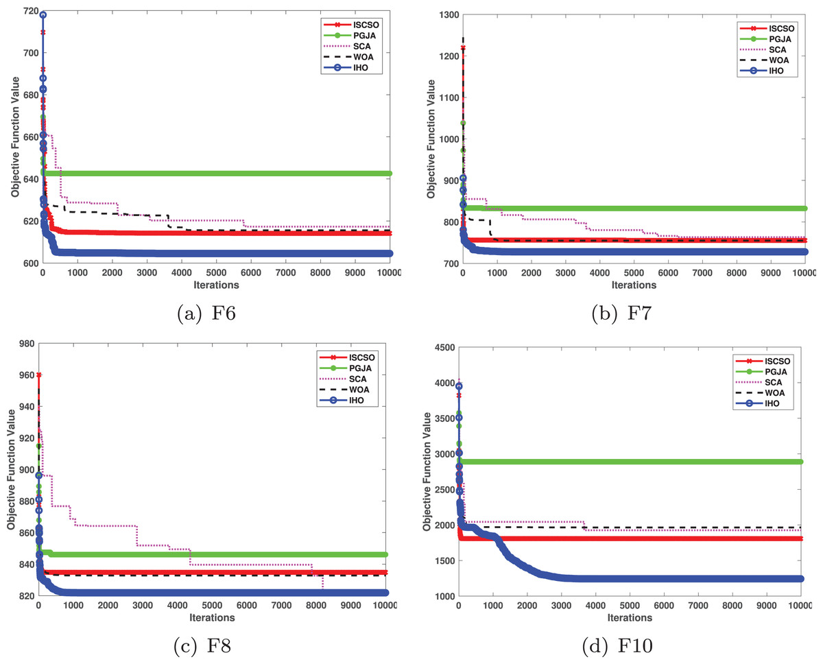
Figure 8: Convergence curves of five algorithms in each benchmark functions (CEC17 D10).
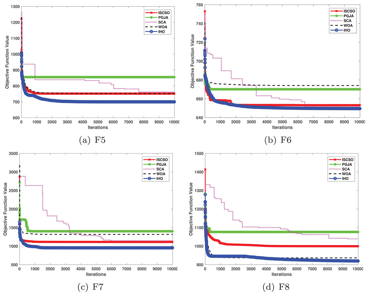
Figure 9: Convergence curves of five algorithms in each benchmark functions (CEC17, D30).
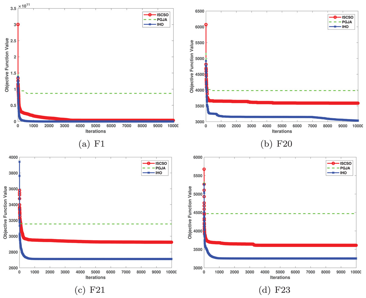
Figure 10: Convergence curves of three algorithms in each benchmark functions (CEC17, D50).
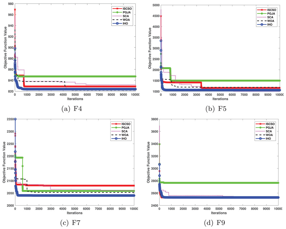
Figure 11: Convergence curves of five algorithms in each benchmark functions (CEC22, D10).
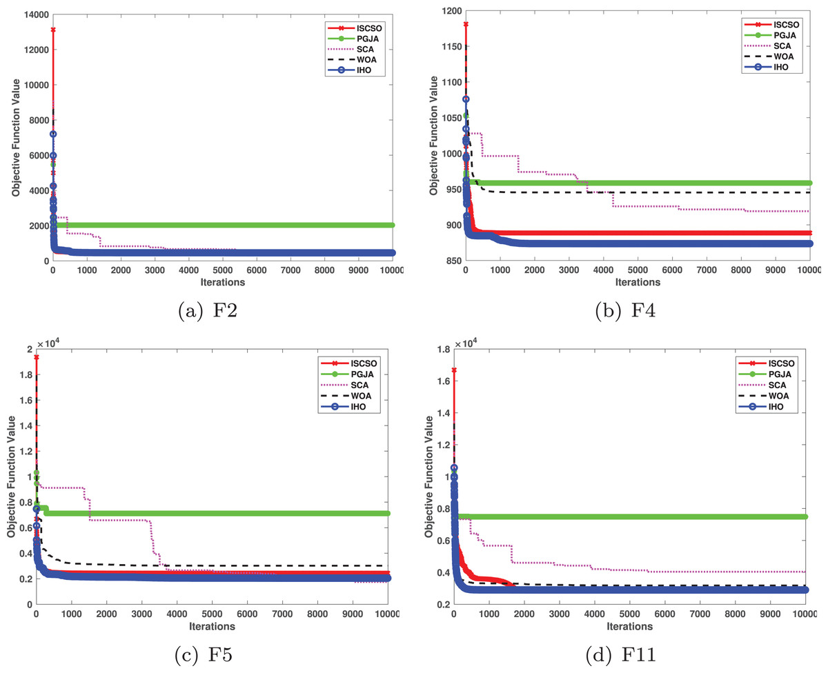
Figure 12: Convergence curves of five algorithms in each benchmark functions (CEC22, D20).
The speed reducer problem (Eq. (17)) aims to minimize the total weight by adjusting parameters such as gear module, teeth number, and shaft length, while meeting stress, deformation, and gear ratio constraints. It involves mixed-integer nonlinear programming (e.g., integer teeth counts) and is a classic case in mechanical transmission optimization.
(17)
Gear train design problem (Eq. (18)) optimizes gear teeth numbers and modules (discrete variables) to minimize transmission ratio error, subject to geometric constraints (e.g., no undercutting) and material strength limits. It is widely used in multi-stage reducers and robotic joint design.
(18)
Three-bar truss design problem (Eq. (19)) minimizes truss mass by adjusting cross-sectional areas of bars under stress, displacement, and stability constraints. Its nonlinear constraints and narrow feasible domain make it a benchmark for testing optimization algorithms.
(19)
When dealing with three engineering optimization problems, IHO is compared with other classical algorithms, as shown in Table 16. From these observations, we can know that IHO performs better than other algorithms.
| Problem | Metrics | GJO | PGJA | IHO |
|---|---|---|---|---|
| Speed reducer | Mean | 3,002.3409 | 3,410.0096 | 2,983.1335 |
| Worst | 3,012.5920 | 4,127.4708 | 2,992.5352 | |
| Best | 2,996.4256 | 3,189.4433 | 2,894.7444 | |
| Std | 6.1953 | 402.2998 | 18.4221 | |
| Gear train design | Mean | 0 | ||
| Worst | 0 | |||
| Best | 0 | 0 | ||
| Std | 0 | |||
| Three bar truss design | Mean | 263.8969 | 264.0344 | 263.8958 |
| Worst | 263.8976 | 264.2412 | 263.8958 | |
| Best | 263.8961 | 263.9156 | 263.8958 | |
| Std | 0.1242 |
Hyperparameter sensitivity analysis
This subsection also provides a sensitivity analysis of IHO to the hyperparameter N. To examine the sensitivity of HO to hyperparameter N, the proposed algorithm is applied across varying values of N, specifically 20, 30, 50, and 100. These differing values of N are utilized to optimize the performance on benchmark functions F1 to F23. The optimization results are presented in Table 17. The sensitivity analysis of IHO to the hyperparameter N indicates that increasing the number of search agents enhances IHO’s capability in exploring the search space, thereby improving the performance of the proposed algorithm and reducing objective function values.
| Fun | ||||
|---|---|---|---|---|
| F1 | ||||
| F2 | ||||
| F3 | ||||
| F4 | ||||
| F5 | ||||
| F6 | ||||
| F7 | ||||
| F8 | ||||
| F9 | ||||
| F10 | ||||
| F11 | ||||
| F12 | ||||
| F13 | ||||
| F14 | ||||
| F15 | ||||
| F16 | ||||
| F17 | ||||
| F18 | ||||
| F19 | ||||
| F20 | ||||
| F21 | ||||
| F22 | ||||
| F23 |
Analysis of advantages and disadvantages of the improved algorithm
Through a series of standard benchmark functions, this study validates the performance of the improved IHO. The experimental results indicate that the improved algorithm outperforms the standard HO and other common metaheuristic algorithms in both convergence speed and solution accuracy. Notably, IHO demonstrated stronger global search capability on multi-modal functions. The evaluation results are presented in Tables 2–4, and Figs. 2, 5 displays the convergence curves of the three most effective algorithms in optimizing CEC05, CEC17, CEC22 and engineering optimization problems. The key findings are summarized as follows.
IHO consistently outperformed other algorithms in terms of convergence speed across a range of benchmark functions, achieving global optima in multiple cases, demonstrating superior convergence. Additionally, the improved algorithm provided higher solution accuracy compared to the standard HO and other metaheuristic algorithms, particularly in multi-modal optimization problems. Furthermore, IHO exhibited lower standard deviation, indicating greater stability in maintaining solution quality over multiple independent runs.
While IHO demonstrates substantial improvements over HO and other algorithms, some limitations remain, such as parameter sensitivity and the computational cost for large-scale problems. However, the overall performance of IHO shows that it is a promising optimization algorithm for solving complex optimization problems.
Conclusion
In this article, we introduced an improved version of the hippopotamus optimization algorithm by implementing three key modifications to enhance its performance. The first modification introduces a gradual reduction of the inertia weight, which helps balance the exploration and exploitation phases, allowing the algorithm to search the solution space more efficiently. The second modification involves adaptively adjusting the mutation rate based on the iteration count, improving the precision of the search in the later stages and reducing the risk of premature convergence. Finally, the predator escape phase has been refined with local boundary updates and position adjustments, resulting in significantly improved global convergence and a greater ability to avoid local optima.
The improved HO was benchmarked on a set of optimization problems, where its performance was compared against the original HO and several well-known metaheuristic algorithms. Results demonstrated that the improved HO consistently achieved superior solutions with higher accuracy, while effectively avoiding common issues such as getting trapped in local minima. The adaptive mechanisms incorporated into the algorithm improved its balance between exploration and exploitation, particularly in complex, high-dimensional search spaces.
Comparative experiments on functions (CEC05, CEC17 and CEC22), using metrics like mean, variance, median, p-value, convergence curves, and box plots, confirmed the enhanced performance of the modified HO over the original and other algorithms. These results highlight the effectiveness and robustness of the proposed improvements in addressing diverse optimization challenges.
In conclusion, the proposed enhancements to the HO algorithm have demonstrated their ability to significantly improve global optimization performance. Future work could explore further extensions of this algorithm, including multi-objective or binary versions, and investigate its application to a wider range of real-world optimization problems across various domains.